On the Quadratic Programming Solution for
Model Predictive Control with Move Blocking
Abstract
Model Predictive Control (MPC) is a popular optimization-based control technique. MPC is usually formulated as sparse or dense Quadratic Programming (QP). This paper reviews two well-known methods, namely, state condensing and move blocking, and brings them together. Their combination results in generalized QP that serves arbitrarily sparse (or dense) QP for MPC with move blocking. The proposed QP can be solved by a specialized solver capable of exploiting a sparsity structure of the problem. Numerical examples give inside in computational and memory requirements.
Index Terms:
Model Predictive Control; Box-Constrained Quadratic Programming; Move Blocking; State CondensingI Introduction
MPC (MPC) is a popular multivariable control technique that systematically incorporates physical constraints (e.g., potential or flow limits) by design. It is an optimization-based method, i.e., in every sampling period, a finite optimal control problem needs to be solved. For linear dynamics and quadratic costs, the problem to be solved is structured QP (QP). For nonlinear dynamics and nonlinear costs, the problem to be solved is NLP (NLP). NLP can be solved by SQP (SQP), which requires a sequence of structured QP to be solved. Therefore, the results presented in this paper can address nonlinear MPC as well.
The two most common QP formulations in which the MPC problem can be written are the dense and the sparse formulation [9]. In the sparse QP formulation, the minimization variables are inputs and states over the prediction horizon, and they are interconnected by the equality constraint representing system dynamics explicitly. Consequently, the QP problem is large in a number of variables with a specific sparsity pattern. On the other hand, in the dense QP formulation, the minimization variables are inputs over the prediction horizon only, the states are eliminated out, and the interconnection is held implicitly. Consequently, the QP problem is smaller, but with no sparsity pattern.
A comparison between sparse and dense QP formulation in the context of walking motion generation is presented in [4]. This application benefits from the use of sparse QP formulation as parameters change in their model; only a negligible additional computational effort is required. In some other applications (e.g., [15]), it might be beneficial to transform sparse QP to the dense one by a so-called condensing procedure. When a model is fixed, the condensing can be performed once offline, which leads to a significant computational saving. Note that condensing can be done with quadratic complexity in horizon length, as proposed in [7].
It should be noted that dense QP can be solved by a generic-purpose solver, which made the dense formulation more popular in the past. Nowadays, several structure-exploiting methods tailored for sparse QP arising in MPC exist (e.g. [20, 6, 13, 19]). As the problem formulation proposed in this work is derived from the sparse QP, these algorithms can be applied with no additional modification required.
When treating dense formulation, the computation complexity can be decreased by the move-blocking technique. The idea of this technique is to fix consequent inputs at the same value. Therefore the number of degrees of freedom of the optimization problem decreases. Another strategy to reduce the number of degrees of freedom is to utilize LQR (LQR) [14]. A move-blocking strategy can optimize control performance, robustness, or feasibility when hard state constraints are considered [17, 18, 8]. The idea of using move blocking regardless of the sampling period was proposed in [5].
State condensing has been proposed in [1]. It enables sparsity level control of the QP formulation. The level of sparsity can be controlled smoothly in between the sparse (non-condensed) to dense (fully-condensed) QP formulation. This method was used for sped-up dual Newton step algorithm regarding nonlinear MPC in [11] or combined with the partial sensitivity update in [2] recently.
To the best author’s knowledge, a generalization of the state condensing for MPC problem with move blocking has not been reported in the literature. From the other way around, move blocking has not been adapted for the sparse QP formulation yet. This paper attempts to address this issue.
The rest of the paper is organized as follows. In Section II, the MPC problem is introduced. Section III gives a basic QP problem formulation of the MPC. In Section IV and Section V, move-blocking and partial-condensing procedures are described, respectively. Section VI presents a QP transformation combining state condensing with move blocking. Section VII gives an insight in computational and memory requirements of the proposed method based on simulations.
II Model Predictive Control
We are concerned in a discrete-time LTV (LTV) systems in the form
where , , and at every time are known. are deterministic, possibly arising from the linearization of nonlinear system. Input and state dimensions are denoted by and , respectively.
Then the problem of the regulator with input box constraints can be treated as the following LTV MPC
| (1a) | |||||
| s.t. | (1d) | ||||
where is a current state measurement (estimation) at time , is the finite prediction horizon length. For the sake of brevity, subscript denotes time period from the sampling moment . For example, and denote the state and input at stage on prediction horizon, respectively. The quadratic weights are , , and the terminal weight . The optimizer of problem (1) is a unique input sequence with associated state trajectory.
As there is new measurement and time-varying model along the prediction horizon is available at each sampling instant, the problem (1) has to be reoptimized. Hence, the receding horizon concept is established, i.e., the plan of control inputs is recomputed at each sampling instant parametrized by measured system state and only the first control move is actually applied to the system, cf. [12]. The need for re-computation requires a fast solver for problem (1), to have a solution ready by the next sampling time.
III Sparse QP Formulation
Problem (1) can be rewritten straightforwardly as a box-constrained QP in the following form
(2a)
s.t.
(2b)
(2c)
parametrized by where denotes box-constrained inputs sequence and denotes states trajectory vectors stacked as
Presented class of problems defined by (2) does impose box input constraints. It is motivated by the fact that algorithm controls actuators, in common, which operate in a limited range (e.g., valve position) or limited range for rate of change (e.g., valve transition speed). The benefit is that box-constrained QP can be solved faster than a generally-constrained one. The presented approach does not impose hard state constraints. It prevents the feasibility issue. However, state limits can be imposed as soft constraints using the penalty method [10]. We believe that the class of problems defined by (2) is wide enough to cover the majority of industrial problems.
The assumption that have been made is
is positive semidefinite. The individual vectors and matrices in (2a) are composed as follows
with a constant term which does not influence the minimizer. The system dynamics (2b) and box-constraints (2c) are given by
Notice that is invertible by construction.
In the following, move-blocking and partial-condensing procedures are recalled. Then they are both incorporated in transformation in Section VI, leading to the generalized QP formulation.
IV Move Blocking
MB (MB) is commonly used to deal with the computational burden in optimal control. The strategy is to fix an input or a change between two consecutive inputs to be constant for several time-steps [14]. Thus, the number of degrees of freedom in the optimization problem is reduced significantly for dense QP formulation.
The choice of the blocking strategy to provide robust control performance is provided in [17], where a generalized blocked variable-horizon MPC is formulated. The optimal blocking strategy is proposed in [18]. Therein, the optimality is measured regarding controller complexity and region of attraction volume and requires a solution to mixed-integer programming. Once a move-blocking strategy is chosen, however, it hasn’t been shown how to decrease the degree of freedom in the optimization problem for sparse QP formulation.
The level of blocking is parametrized by move-bloking vector , where are sizes of blocking windows and is number of input vectors after blocking to be optimized, and for which . For sake of brevity, an auxiliary vector of row indicies 11
1
Function cumsum returns vector of cumulative sum of input argument. is defined. Then blocking matrix and and input vectors after blocking to be optimized are
respectively. The blocking is provided by input transformation
| (3) |
Note that is matrix of ones and zeros only such that . For the admissible , an identity on each following row must be in the same column or the next right column. Move blocking approximates the original problem with one with a lesser number of degrees of freedom. The approximation effect on the control performance has been discussed, e.g., in [16]. Therein, the authors suggest a heuristic method to adapt the blocking strategy online such that control performance remains nearly unchanged. This paper focuses rather on computational and memory aspects.
In this paper, we modify [1] to allow the state condensing works for move-blocked MPC.
V State condensing
The state condensing was introduced in [1]. The idea is to eliminate not every, but only some of the state vectors from along the prediction horizon. This will result in an optimization problem where equality constraints representing system dynamics are eliminated out only partially. The idea is to take advantage of both sparse and dense QP formulation, as in the partially-condensed problem, some sparsity structure remains, and simultaneously, the number of variables is reduced.
The level of condensing is parametrized by a state condensing vector , where are sizes of condensing windows and is number of states vectors after condensing. For sake of brevity, a vector of row indicies is defined. Possible option is , i.e. is empty vector which results in dense formulation. Then condensing matrix and state vectors after condensing to be optimized are
respectively. The remaining states and states being condensed out are separable as
| (4) |
where
The prediction (2b) can be decomposed on the rows related to the remaining states using and the rest using , respectively, as
| (5) | ||||
| (6) |
Adding (4) to (6) a partial state prediction can be written down
| (7) |
where
The state condensing exploits banded structure of . For the sake of brevity, the structure of the matrix follows
Note that remains invertible, moreover, is also unit lower triangular for any admissible .
(8)
Note that for fully sparse case implies are empty matrices of particular size, i.e. the transformation is not needed at all. On the other hand, for dense case implies and (V) yields an ordinary prediction. Further, only (5) and (V) are going to be used.
State condensing transform the original problem into an equivalent one of a smaller dimension. The state-condensing procedure benefits from the fact that is block-diagonal. Therefore, it can be computed block by block, and off-diagonal terms remain zero.
VI Generalized QP Formulation
By interconnectiong both previous methods, namely move blocking (3) and state condensing (4),(V), a systematic transformation can be written down now
| (10a) | ||||
| (10b) | ||||
where and .
The problem (2) can be then transformed using (10) into a generalized QP (11) of the similar structure. The transformation (10) is applied on (2) such that (10a) and (10b) are substitute in (2). Then the resulting generalized QP problem is
| (11) | |||||
| s.t. | |||||
where
(12)
and where denotes left-inverse of . When the data for (2) are available a generalized QP formulation QP (11) is given by (12) parametrized by and . Matrices in (12) can be build efficiently with respect the sparsity structure and FLOPs (FLOPs) count can be obtained easily. Remember, any admissible choice of blocking matrix (except ) causes (11) approximates (2) by problem with less degree of freedom. On the other hand, any admissible does not affect the minimization result.
Problem (11) can be solved efficiently by an active-set or an interior-point method. Note that both and Cholesky decomposition typically used to find a Newton step within any of these methods preserves the sparsity pattern of this problem.
VII Numerical Examples
For the sake of brevity, transformation matrices for a short prediction horizon problem setup are shown first. It is followed by a common benchmark – the oscillating masses controlled by move-blocked MPC with a given blocking strategy. Finally, for a given system and prediction horizon, the whole transformation space is sampled to demonstrate the behavior of the proposed problem setups in more detail.
VII-A Illustrative Example
Assume a random LTV system with ten states () and five inputs () for which sequence of move blocks was given to be , consequently, . Prediction horizon is and control horizon is . Let’s choose to be similar to the in the first entries, consequently, . In this case, the transformation matrices in (3) and (4) are given by
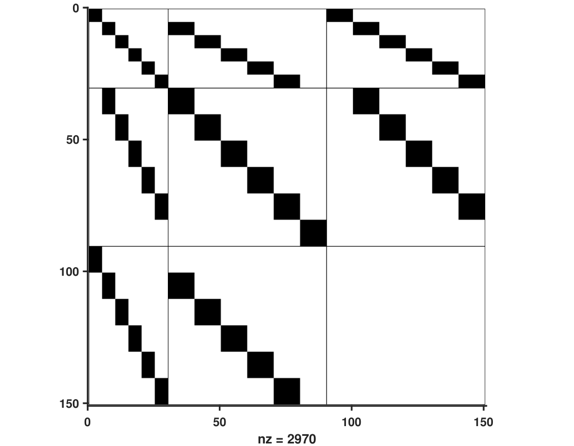
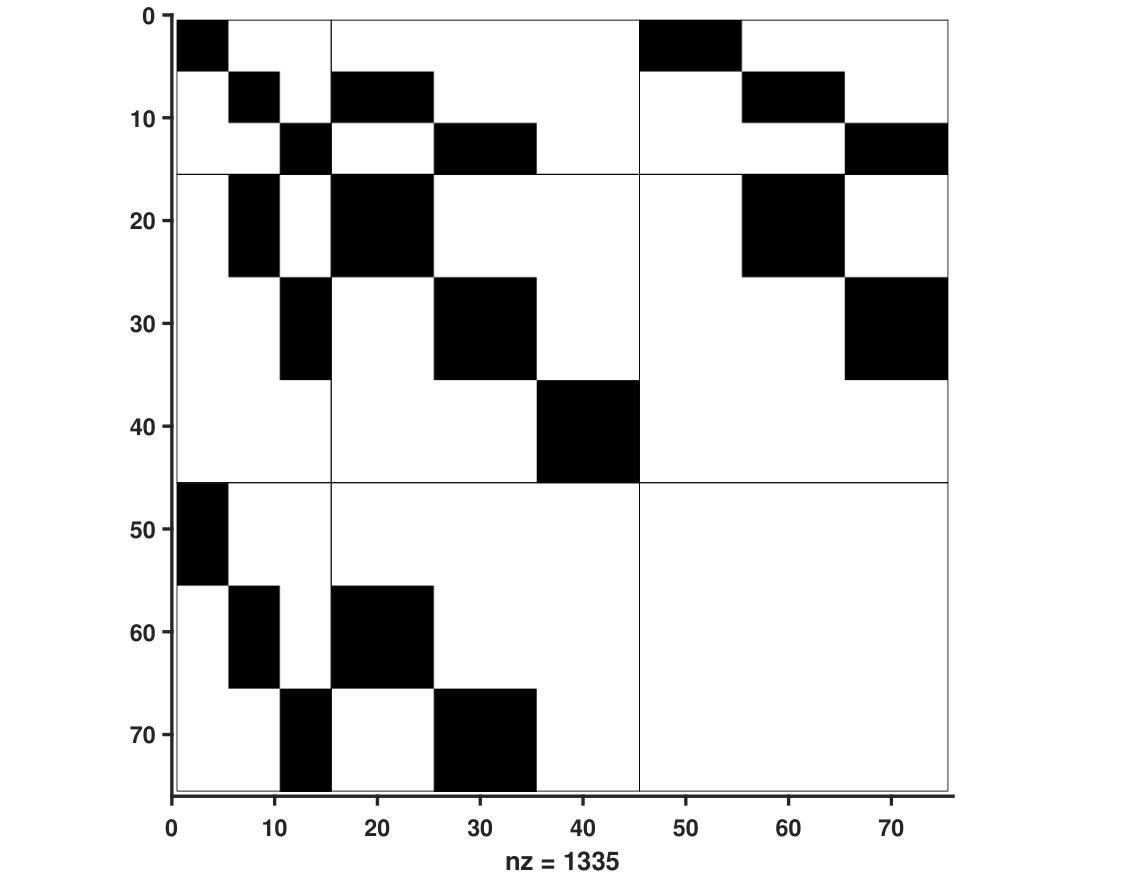
The sparsity structure of the resulting QP problem can be demonstrated at the KKT (KKT) matrix of QP problem (11) with no inequality constraints being activated. The associated KKT matrix is
| (13) |
This simple example illustrates (see Fig. 2) that the structure pattern of the problem is invariant for the proposed transformation. Also notice, the transformed problem has a smaller dimension, and less than half non-zero elements; therefore, it is expected the transformed problem requires less computational effort to a solution.
VII-B Oscillating Masses
This benchmark is inspired by [20]. The proposed system consists of a sequence of six masses connected to each other by spring dampers. The first and the last masses are connected to the walls. The weight of each mass is kg and the spring constant is N/m without damping. The system state represents the displacement and velocity of an individual mass. There are four control inputs, i.e., , which exert tensions between different masses. We assume control limits , and the presence of random bounded external disturbance with a uniform distribution on , which acts additionally on the displacement state of each mass. The control objective is to stabilize each mass in its origin, i.e., to solve (1) with , , , , , and with sampling time s.
Further, we focus on the computational cost of problem (11) build (preparation phase) and its solution (feedback phase). This is typically studied in nonlinear MPC, where (11) has to be built and solved every sampling period [3]. The more QP problem is condensed and/or blocked, the more expansive the preparation is. On the other hand, the preparation may sufficiently decrease the solution time in particular. The preparation and feedback phase for some specific cases are examined numerically, and FLOPs are measured.
The feedback phase denotes the cost of problem (11) solution, in this paper, it is counted for NPPsparse solver [13]. This active-set-like method converges typically in several iterations. The method benefits from the use of warm/hot-start while the number of iterations is insensitive to the problem conditioning.
In this exemplary case, the move-blocking strategy was chosen to be
Once the blocking strategy is fixed, the control performance is immutable, i.e., all examined QPs are equivalent. For this setup, various levels of condensing are tested. Condensing vector is chosen such that any state vector is closing move-blocking series, more precisely
and
where in the later some of the block windows are additionally splitted in half to obtain the proper length of vector . Resulting computational and memory requirements for this setup are shown in Fig. 3.
In Fig. 3, on the left () is the sparse QP and on the right () is the dense problem formulation. The first observation is that minimal computational or memory burden is in between these two. In other words, it is beneficial to condense the original sparse QP partially. Specifically, computational requirements of the optimally condensed (FLOPs) compared to the dense QP (FLOPs) is more than three times lower. One can save of memory space in case of optimally condensed ( NNZs (NNZs)) compared to the dense QP (NNZs). Another observation is that preparation cost when no condensing is required is significantly smaller compared to any other level of condensing.
In general, the computational cost of the preparation phase grows with the level of condensing. On the other hand, the computational cost of the feedback phase is not monotone and changes depending on multiple factors () and importantly, on a particular algorithm implementation.
The presented numerical experience illustrates that using generalized QP formulation (11), for a given move-blocked MPC, an optimization problem that requires minimal FLOPs can be found.
The proposed approach has been implemented and tested in MATLAB environment, which allows code generation to an embedded platform. There is no need for two separate pieces of code (for dense and sparse QP formulation), which labor-saving of code maintenance.
VIII Conclusion
In this paper, we combine move-blocking and state-condensing procedures in generalized QP formulation of a move-blocked MPC problem. The combination of move-blocking and state-condensing methods allows reducing the number of input variables as well as a number of state variables. This approach allows for a MPC with a given move-blocking strategy to find such a QP formulation for which a total computational burden or memory footprint of the MPC regulator is minimal. It has been illustrated how the proposed transformation affects memory footprint and computational burden by numerical examples. We analyzed on the example, the computational burden could be significantly decreased () or memory saved (). The proposed approach requires specialized QP solver used together with an optimized library for sparse linear algebra.
References
- [1] Daniel Axehill. Controlling the level of sparsity in mpc. Systems & Control Letters, 76:1–7, 2015.
- [2] Yutao Chen, Gianluca Frison, Niels van Duijkeren, Mattia Bruschetta, Alessandro Beghi, and Moritz Diehl. Efficient partial condensing algorithms for nonlinear model predictive control with partial sensitivity update. IFAC-PapersOnLine, 51(20):406 – 411, 2018. 6th IFAC Conference on Nonlinear Model Predictive Control NMPC 2018.
- [3] Moritz Diehl, Hans Georg Bock, and Johannes P. Schlöder. A real-time iteration scheme for nonlinear optimization in optimal feedback control. 43(5):1714–1736, 2005. Exported from https://app.dimensions.ai on 2018/12/13.
- [4] Dimitar Dimitrov, Alexander Sherikov, and Pierre-Brice Wieber. A sparse model predictive control formulation for walking motion generation. In IEEE/RSJ International Conference on Intelligent Robots and Systems, IROS 2011, September, 2011, pages 2292–2299, San Francisco, Etats-Unis, sep 2011. IEEE.
- [5] M. Faroni, M. Beschi, M. Berenguel, and A. Visioli. Fast mpc with staircase parametrization of the inputs: Continuous input blocking. In 2017 22nd IEEE International Conference on Emerging Technologies and Factory Automation (ETFA), pages 1–8, 2017.
- [6] Janick V. Frasch, Milan Vukov, Hans Joachim Ferreau, and Moritz Diehl. A new quadratic programming strategy for efficient sparsity exploitation in sqp-based nonlinear mpc and mhe. IFAC Proceedings Volumes, 47(3):2945 – 2950, 2014. 19th IFAC World Congress.
- [7] Gianluca Frison. Algorithms and methods for high-performance model predictive control. 2016.
- [8] Ravi Gondhalekar and Jun ichi Imura. Least-restrictive move-blocking model predictive control. Automatica, 46(7):1234 – 1240, 2010.
- [9] Juan L Jerez, Eric C Kerrigan, and George A Constantinides. A condensed and sparse qp formulation for predictive control. In Decision and Control and European Control Conference (CDC-ECC), 2011 50th IEEE Conference on, pages 5217–5222. IEEE, 2011.
- [10] Eric C. Kerrigan and Jan M. Maciejowski. Soft constraints and exact penalty functions in model predictive control. In Proc. UKACC International Conference Control, 2000.
- [11] D. Kouzoupis, R. Quirynen, J.V. Frasch, and M. Diehl. Block condensing for fast nonlinear mpc with the dual newton strategy. IFAC-PapersOnLine, 48(23):26 – 31, 2015. 5th IFAC Conference on Nonlinear Model Predictive Control NMPC 2015.
- [12] D Mayne, J. B. Rawlings, C. V. Rao, and P. O. M. Scokaert. Constrained model predictive control: Stability and optimality. Automatica J. IFAC, 36(6):789–814, 2000.
- [13] Pavel Otta, Jiří Burant, Ondřej Šantin, and Vladimír Havlena. Newton projection with proportioning using iterative linear algebra for model predictive control with long prediction horizon. Optimization Methods and Software, 34(5):1075–1098, 2019.
- [14] Cagienard Raphael, Grieder Pascal, Kerrigan Eric C., and Manfred Morari. Move blocking strategies in receding horizon control. Journal of Process Control, 17(6):563 – 570, 2007.
- [15] Stefan Richter, Sebastien Mariethoz, Manfred S. Richter Morari, S. Mariéthoz, and M. Morari. High-speed online mpc based on a fast gradient method applied to power converter control. In Proceedings of the 2010 American Control Conference, pages 4737–4743, June 2010.
- [16] T. Schwickart, H. Voos, M. Darouach, and S. Bezzaoucha. A flexible move blocking strategy to speed up model-predictive control while retaining a high tracking performance. In 2016 European Control Conference (ECC), pages 764–769, June 2016.
- [17] Rohan C. Shekhar and Jan M. Maciejowski. Robust variable horizon mpc with move blocking. Systems & Control Letters, 61(4):587 – 594, 2012.
- [18] Rohan C. Shekhar and Chris Manzie. Optimal move blocking strategies for model predictive control. Automatica, 61:27 – 34, 2015.
- [19] F. Ullmann. FiOrdOs: A Matlab toolbox for C-code generation for first order methods. Master thesis, Swiss Federal Institute of Technology Zurich, ETH, Zurich, 2011.
- [20] Yang Wang and Stephen Boyd. Fast model predictive control using online optimization. IEEE Trans. Control Syst. Technol., 18(2):267–278, 2010.