Enhanced spectrum of primordial perturbations, galaxy formation and small scale structurePreprint: APS/123-QED
Abstract
The standard cosmological structure formation scenario is successful on large scales. Several apparent problems affect it however at galactic scales, such as the small scale problems at low redshift and more recent issues involving early massive galaxy and black hole formation. As these arise where complex baryonic physics becomes important, this is often assumed to be behind the problems. But the same scales are also those where the primordial spectrum is relatively unconstrained, and there are several ways in which it can be modified. We focus on that arising from effects possibly associated with the crossing of high energy cutoff scale by fluctuation modes during inflation. Elementary arguments show that adiabatic evolution cannot modify the near scale invariance, we thus discuss a simple model for the contrary extreme of sudden transition. Numerical calculations and simple arguments suggest that its predictions, for parameters con2sidered here, are more generic than may be expected, with significant modifications requiring a rapid transition. We examine the implications of such a scenario, in this simplest form of sudden jump as well as gradual variants, on the matter power spectrum and halo mass function in light of the limitations imposed by particle production. We show the resulting enhancement and oscillation in the power spectrum on currently nonlinear scales can potentially simultaneously alleviate both the apparent problem of early structure formation and, somewhat counterintuitively, problems at low redshift concerning the abundance of dwarf galaxies, including those too big to fail. We discuss consequences that can observationally constrain the scenario and its parameters, including an inflationary Hubble scale , while touching on the possibility of simultaneous modification of power on the largest scales.
I Introduction
Structure can condense from small density perturbations in a nearly homogeneous universe through gravitational instability. In the context of contemporary cosmology the density perturbations are seeded by quantum fluctuations in a primordial scalar field driving inflation, which later decays as the universe reheats and the standard model particles (and putative dark ones) arise (e.g., Lyth and Liddle 2009; Peter and Uzan 2009). The statistical properties of the primordial perturbations thus leave their mark on the cosmic microwave background (CMB) and large scale structure of the galaxy distribution. On these scales, on which they can be inferred with precision, the properties of the perturbations are consistent with a nearly scale invariant primordial spectrum essentially determining their statistics Planck Collaboration et al. 2018.
At a phenomenological level, the simplest models of inflation do predict a near scale invariant primordial power spectrum if the inflaton potential is specified in such a way that the resulting Hubble parameter is nearly constant over a sufficient number of e-folds. Nevertheless, this prediction is not unique Salopek et al. 1989; Dodelson and Stewart 2002; indeed, little is known of the microscopic physics of inflation, or the wider particle physics model it may be a part of, and the coupling of the inflaton driving inflation to other fields may lead to changes in the potential that can ruin the predictions of standard slow roll models (.e.g., Adams et al. 1997; Chung et al. 2000; Burgess et al. 2003; Romano and Sasaki 2008 and Lyth and Riotto 1999; Yamaguchi 2011; Baumann and McAllister 2015 for reviews). Stages of singular or rapid evolution of the potential or its derivatives, interrupting slow roll, leave imprints on the primordial spectrum of fluctuations Starobinskij 1992; Polarski and Starobinsky 1992; Adams et al. 2001; Chung et al. 2000; Lesgourgues 2000; Yamaguchi 2001a; Feng et al. 2003; Elgaroy et al. 2003; Gong 2005; Dvorkin and Hu 2010; Namjoo et al. 2012. Such effects may lead to a variety of ’features’ and changes that break the scale free spectrum, and may have observable consequences associated with significant enhancement or suppression of power on large scales Lesgourgues et al. 1998; Gramann and Hütsi 2000; Gramann and Hütsi 2001; Contaldi et al. 2003; Gong 2005; Sinha and Souradeep 2006; Joy et al. 2009, as well as on smaller (galactic and sub-galactic) scales Kamionkowski and Liddle 2000; Yokoyama 2000; Zentner and Bullock 2002; Little et al. 2003; Enqvist et al. 2019; Berezinsky et al. 2010; Leo et al. 2018, including the formation of primordial black holes Yamaguchi 2001b; Bringmann et al. 2002. However the anomalous variation in the inflaton potential needs to be localized in order for single field slow roll inflation to proceed for a sufficient number of e-folds, and is also limited on large scales by observations suggesting a nearly scale invariant primordial power spectrum Easther and Peiris 2006; Planck Collaboration et al. 2018.
In some models, such as DBI inflation, the breaking of scale invariance and associated features in the power spectrum are best represented in terms of sharp temporal variations in the sound speed of perturbations Bean et al. 2008; Nakashima et al. 2011; Miranda et al. 2012; Miranda and Hu 2014; Park and Sorbo 2012; Gariazzo et al. 2017; Ballesteros et al. 2019. This is still accompanied by corresponding changes in the equation of state of the inflaton and therefore, as in the cases above, by anomalous background evolution. On the other hand, if inflation proceeds modestly longer than the minimal number of e-folds needed to solve problems such as the apparent causal connection in the CMB field (’horizon problem’), primordial perturbations are expected to arise from well within a high energy cutoff scale where new physics may transpire. This gives rise to what is often termed as the trans-Planckian problem. The minimal length scale that it entails can be introduced by modifying the commutation relations or introducing nonlinear dispersion relations for the propagation of fluctuations (early studies include Martin and Brandenberger 2001a; Brandenberger and Martin 2001; Easther et al. 2001; Niemeyer 2001; Martin and Brandenberger 2003; Easther et al. 2005a; Kempf and Lorenz 2006, while a relatively recent review can be found in Brandenberger and Martin 2013).
If the Hubble scale of inflation is smaller than the scale , where new physics may appear, the background evolution is unmodified by possible new physics; modifications to the scale invariant spectrum may then arise solely from anomalous evolution of the fluctuation modes, rather than of the inflation potential. However, if some form of decoupling is assumed — e.g. motivated by the fact that the power spectrum is evaluated at horizon exit scales — then the corrections can be quite small; of order , with . In the context of local effective field theory Kaloper et al. 2002; if the fluctuation modes are assumed to simply emerge from the quantum foam at conformal time , depending on the comoving mode wavenumber — instead of the usual Bunch Davies initial conditions taken at — then Danielsson 2002; Easther et al. 2002; if the modes emerge from the local adiabatic vacuum then Niemeyer et al. 2002. A covariant small scale cutoff, introduced by removing field configurations that are off shell by more than a Planck scale leads to Chatwin-Davies et al. 2017.
Much larger corrections are nevertheless possible in principle. This is the case, in particular, if the emergence of the inflating modes from the high energy cutoff scale is assumed to be preceded by non-adiabatic evolution arising from a nonlinear dispersion relation at scales Martin and Brandenberger 2001a; Brandenberger and Martin 2001; Brandenberger and Martin 2002; Zhu et al. 2016; Ashoorioon et al. 2017. Modes then do not emerge from the foam in their lowest energy states. Excited states arise, providing anomalous initial conditions for further evolution and leading to enhancement and oscillations in the power spectrum. The most general parametrization of the effects of a non-adiabatic high energy scale exit would therefore appear to include both phenomena Martin and Brandenberger 2003; Armendariz-Picon and Lim 2003.
Though physics at these scales is largely unknown, it can in principle be envisioned that the introduction of a cutoff scale in itself can modify the effective dynamics of the fluctuations. Indeed, the introduction of a minimal length scale and a large variety of phenomenological descriptions of ’quantum spacetimes’, can be characterized by nonlinear dispersion relations Amelino-Camelia 2013; Hossenfelder 2013. At the most intuitive level, a simple hydrodynamic analogy suggests such a modification to the propagation of fluctuations Unruh 1981; Unruh 1995; Barcelo et al. 2005. This, much in the same way that an effective macroscopic description of wave propagation through a fluid or lattice may still be employed at wavelengths approaching the interparticle distances, provided this is phenomenologicaly taken into account through a modified dispersion relation. As, at scales smaller than the interparticle distances waves cannot propagate at all, it is in the transition between such a cutoff scale and the scale on which the standard effective macroscopic description applies that a nonlinear dispersion relation may describe the propagation of fluctuations. At this simplest intuitive level, one may expect the dynamics of a sound wave, initially moving in a medium where interparticle spacing is large and comparable with its wavelength, to keep memory of the anomalous evolution, even after it crosses and propagates into a medium with smaller interparticle spacing, where the effective theory is perfectly valid and ’decoupling’ is guaranteed. The rough analogy here would be with an inflaton fluctuation mode inflating from wavenumbers above the high energy cutoff scale to ones below it, on its way to the horizon. Applications of more sophisticated ’analogue’ models to the inflationary scenario show that modifications of the dispersion relation can indeed lead to significant changes of power spectrum of field correlations Chä and Fischer 2017.
An important limitation on modifications of the power spectrum through the inclusion of excited states relates to the fact that these are necessarily associated with departures from a vacuum state. And too much excitation can lead to departures significant enough to prohibit inflation from starting and persisting in the first place Tanaka 2000; Niemeyer and Parentani 2001; Starobinsky 2001; Giovannini 2003; Porrati 2004. However, as has been pointed out, the limitations that arise thus may not be very constraining Greene et al. 2005; Brandenberger and Martin 2005; Danielsson 2005. In the present investigation we wish to examine whether, within the limits imposed by particle production, excitations of inflaton modes, stemming from the presence of high energy cutoff scale, can lead to significant and astrophysicaly interesting modifications of the primordial power spectrum.
At present, the non-observation of significant departures from scale invariance on large (linear) scales, where the primordial spectrum can be rather precisely inferred, seem to embody the main evidence against such modifications. Indeed, observations on scales on which the density perturbation is linear preclude even relatively small modifications Goldstein and Lowe 2003; Easther et al. 2005b; Okamoto and Lim 2004; Martin and Ringeval 2005; Martin and Ringeval 2004. Observations are however much less constraining at smaller scales, where they are limited by the Silk damping of the CMB, and by nonlinear structure formation erasing the possibility of directly mapping the observed power spectrum to the primordial one. Precise CMB and large scale structure inference is therefore limited to scales . For a horizon scale of this spans three orders of magnitudes. More model dependent constraints are available from the Lyman- forest down to wavenumbers roughly corresponding to comoving spatial scales of order of Mpc. Beyond that, the spectrum is currently quite weakly constrained Chluba et al. 2012a; Chluba et al. 2012b; Emami and Smoot 2018. On the other hand, the smallest structures that form in the context of the standard cold dark matter scenario have earth mass and roughly solar system size . From such scales to the smallest scales at which the linear power spectrum can be directly recovered one counts 11 orders of magnitude — nine more than those separating the nonlinear scale to the horizon.
It is not inconceivable that the scale invariance of the primordial power spectrum does not hold in some parts of the aforementioned range. On the contrary, despite the significant successes of the current model of structure formation on large scales Frenk and White 2012, through the past couple of decades a variety of problems have arisen on galactic scales. There is a group of quite possibly related longstanding issues connected to the central densities of dark matter halos, and the abundance and dynamical properties of local dwarf galaxies Del Popolo and Le Delliou 2017; Bullock and Boylan-Kolchin 2017; and, in apparent contradiction, more recent issuees related to an apparent preponderance of massive old galaxies and supermassive black holes at redshifts that may pose a challenge the current CDM-based structure formation paradigm De Rosa et al. 2014; Wu et al. 2015; Watson et al. 2015; Hirano et al. 2015; Steinhardt et al. 2016; Valiante et al. 2016; Stefanon et al. 2017; Glazebrook et al. 2017a; Venemans et al. 2017; Behroozi and Silk 2018; Tang et al. 2019; Cecchi et al. 2019; Smith and Bromm 2019; Wang et al. 2019.
Such problems appear in the highly nonlinear regime of structure formation; where small density perturbations, born of primordial ones in the presumed inflaton, have sufficiently grown under gravity to form gravitationaly bound objects. Since it is also at such scales that complex baryonic physics becomes important, it was natural to suppose that the main determinant lies in complex baryonic physics of galaxy formation and evolution. For example, for the small scale problems at , processes involving energy input to dark matter halos through dynamical friction with baryons El-Zant et al. 2001; El-Zant et al. 2004; Romano-Díaz et al. 2008; Goerdt et al. 2010; Cole et al. 2011; Inoue and Saitoh 2011; Laporte and White 2015; Nipoti and Binney 2015; Del Popolo et al. 2018 or through random potential fluctuations driven by starbursts or active galactic nuclei (AGN) Read and Gilmore 2005; Mashchenko et al. 2008; Peirani et al. 2008; Pontzen and Governato 2012; Teyssier et al. 2013; Pontzen and Governato 2014; El-Zant et al. 2016, were invoked. (In addition to suggestions modifying the dark matter particle physics models, as in warm dark matter Colín et al. 2000; Bode et al. 2001; Macciò et al. 2012; Lovell et al. 2014; El-Zant et al. 2015, self interacting dark matter Spergel and Steinhardt 2000; Burkert 2000; Kochanek and White 2000; Miralda-Escudé 2002; Zavala et al. 2013; Elbert et al. 2015 and fuzzy dark matter Goodman 2000; Hu et al. 2000; Schive et al. 2014; Marsh and Silk 2014; Hui et al. 2017). Similar attempts are ongoing in the case of the the more recent early structure formation issue (some are discussed in Section IV.3.2).
However, it is also precisely at the nonlinear scales, where baryonic physics becomes important, that the primordial power spectrum is relatively unconstrained. That modifications thereof can be relevant to small scale problems associated with galaxy formation has long been realized Kamionkowski and Liddle 2000, but not as extensively investigated as the baryonic solutions discussed above. While feedback from starbursts and AGN is now recognized as a central ingredient of galaxy formation, independently of its possible role in alleviating the aforementioned issues, and whereas massive baryonic clumps, proposed to mediate dynamical friction coupling to dark matter, have since been observed in forming galaxies (e.g. Genzel et al. 2011; Cava et al. 2018), it is also important to further examine mechanisms that address galactic scale problems through modification of the primordial spectrum. Deriving the consequences of such modifications is in itself an interesting tool for understanding the processes from which they may arise in an inflationary era.
In this study we investigate the effect on the power spectrum from field excitations, stemming from non-adiabatic transition through a high energy cutoff regime corresponding to currently nonlinear scales, and within the limits imposed by particle production. We attempt to do this in generic terms, starting from well defined initial conditions, with linear dispersion relation (but with sound speed different from unity) and examining the effect of the transition. As this solely affects the fluctuation modes, the equation of state of the inflaton, and thus the background evolution, remains unmodified (unlike in cases such as DBI inflation mentioned above), this helps isolate the effect of excitations on the spectrum. We then look for associated effects on the matter power spectrum and dark matter halo mass function.
In the next section, after illustrating in simplest terms how the power spectrum is essentially an adiabatic invariamt of the dynamics of inflaton fluctuations, we present and discuss a simple model representing the other extreme of a sudden transition (in an appendix, we show results that suggest it is generic for a large range of parameters; in a second appendix we discuss the situation when the assumption is relaxed). In Section III we discuss what this model entails in more formal terms, evaluating the limits on power spectrum modification in terms of particle production. In Section IV, we study, within these limits, the possible modifications on the matter power spectrum and halo mass function. We discuss possible astrophysical consequences and constraints, before presenting our conclusions
II Adiabaticity, scale invariance and the sudden extreme
II.1 The evolution of fluctuations
The general quadratic action for inflationary perturbations with sound speed can be expressed in terms of the Mukhanov-Sasaki (MS) variable as Mukhanov et al. 1992; Armendariz-Picon et al. 1999; Garriga and Mukhanov 1999:
| (1) |
where , is the background inflaton field, , and the primes denote derivative with respect to conformal time . The evolution of each Fourier mode is governed by the MS equation
| (2) |
The MS variable is related to the curvature perturbations by . This is a quantity of fundamental interest, as it relates primordial quantum fluctuations to the observables, such as CMB anisotropies; the power spectrum of the large scale galaxy distribution; and, ultimately (more indirectly), the formation of smaller scale structures, such as the dark matter halos hosting galaxies. The dimensionless power spectrum of such perturbations is given by
| (3) |
where the right-hand side is evaluated at the horizon (); as in the absence of isocurvature perturbations, the comoving curvature perturbations are conserved on super-horizon scales Salopek and Bond 1990. Scale-invariant perturbations correspond to . Departures from this can arise if , or the inflationary Hubble scale , depend on time.
In the standard inflationary scenario, a massless field, and quasi de Sitter evolution is assumed (and so is nearly constant throughout the inflationary stage). The associated slow roll parameters, defined as
| (4) |
are always much smaller than unity. Any departure from scale invariance is small, and is usually quantified by the spectral tilt parameter :
| (5) |
The slow roll parameters being small implies that .
To first order in the slow roll parameters, and assuming canonical kinetic terms, one can also show that
| (6) |
In this case, to a good approximation, one can rewrite (2) as
| (7) |
If no non-standard dispersion relation is invoked then , and the standard scenario may be fully recovered.
II.2 Adiabaticity, adiabatic invariants and primordial power spectrum
II.2.1 General context
In the context of equation (2), setting can be interpreted as the result of assuming a massless field with linear dispersion relation between the physical frequency and the physical wavenumber , . However, as discussed in the introduction, this is not a necessity; a modification of the equation of state of the inflaton (e.g. such as in DBI inflation), or modification of the dispersion relation due to modes probing a high energy cutoff scale, beyond which new physics may arise, can change the situation.
In the latter case, beyond a cutoff scale , one can introduce the relevant modification by replacing the square of the comoving wavenumber in (2) with
| (8) |
the main requirement being that the new dispersion relation recovers the linear one for scales Martin and Brandenberger 2001b.This dispersion relation is thus necessarily time dependent, as it must transit between two regimes. It can be used to parametrize and reflect the effect of a varying sound speed in equations (2) and (7), the latter applying when the background dynamics is well approximated by standard slow roll. Indeed, in this context, Eq. (2) can be rewritten as
| (9) |
(A more rigorous derivation, based on a variational principle, can be found hereLemoine et al. 2001).
How does the extra time dependence, that thus arises, affect the power spectrum derived from the above equation? As noticed in several studies, mere time dependence in itself is not sufficient to alter the nearly scale invariant nature of the primordial spectrum of fluctuations. The adiabaticity condition — that is, — must be violated. A well known example where this condition is indeed violated invokes the Corley-Jacobson dispersion relation
| (10) |
(where is a constant and an integer). The studies Martin and Brandenberger 2001b; Martin and Brandenberger 2002; Brandenberger and Martin 2001, indeed indicated that a modification of the power spectrum, in the form of a change in the spectral index and superimposed oscillations, was possible. However, several criticisms were raised, including the possibility of complex frequencies arising at early times, rendering the quantum field theory ill-defined, and problems related to setting the initial conditions in non-adiabatic regime. To circumvent such issues, a new dispersion relation Lemoine et al. 2001 was proposed, which exhibits linear behaviour in the small and large wavenumbers, but has intermediate concave region where the adiabaticity is violated locally.
Here we will be considering a simpler scenario, which assumes standard Bunch Davies type initial conditions, with modified sound speed but still linear dispersion relation. The effective sound speed transits to the standard relation as the boundary around is crossed. In this simple controlled context, we wish to estimate the rapidity and steepness of the transition required in order to produce palpable change in the power spectrum. It turns out that such a transition must be quite rapid.
II.2.2 The power spectrum as an adiabatic invariant
We now wish to show, in explicit simple terms, that the primordial power spectrum is in fact an adiabatic invariant of the evolution of inflationary perturbation, and thus cannot be snigficiantly modified by any changes in the dispersion relation that keeps the dynamics of the perturbations sufficiently adiabatic.
We will be interested in the case when the dispersion relation is modified due to the fluctuation modes probing scales beyond a high energy cutoff, before they inflate into lower energy scales on their way to horizon exit. Only the effective speed of mode propagation is modified and slow roll inflation of a massless field is assumed to hold in all stages. So, Eq. (7) holds to a good approximation. However, because of the non-standard dispersion relation assumed, in that equation will not be necessarily unity in all stages. In fact its variation would incorporate changes parametrized by in Eq. (9) above.
In principle in (7) can be either larger or smaller than unity. Perhaps a scenario in which modes do not propagate at all for , and then do so at increasing as they emerge from the ’quantum foam’ at , is appealing; it qualitatively connects, for example, to waves propagating in a lattice, which are scattered and dispersed to smaller speeds as one approaches the interparticle spacing, before ceasing to propagate. However ’analogue’ models with superluminal speeds , beyond the cutoff scale, have also been proposed Barcelo et al. 2005. As we discuss in Section III, for our purposes both situations lead to similar results.
Equation (7) refers to a simple harmonic oscillator with variable frequency. If is constant, the variation solely comes from the second term in the bracket. To separate this effect from that connected to possible variation in at a high energy cutoff transition, we exploit the fact that . This enables one neglect the second term in the brackets of equation (7), at scales () around the high energy cutoff transition; as, when modes transit from beyond the cutoff scale to below it, the conformal time . The term in the brackets in the aforementioned equation is then . The second term inside this latter bracket is small compared to unity when
| (11) |
Since we already assume that , this is always the case when . We will also assume that this condition is satisfied when considering the case of 11 1 Indeed, as discussed in Section IV.1.2, in order to get modification of the matter power spectrum and halo mass function at scales of the order of a comoving Mpc, which are of particular interest, one needs , much smaller than , which is the smallest we consider..
This leaves us with an equation of a harmonic oscillator with frequency . The adiabatic invariant for a standard harmonic oscillator with specific energy and frequency is . Taking the modulus of the amplitude and the velocity , the energy of the oscillator is . Whatever the evolution at scales above , as long as it is adiabatic is conserved. Moreover, at scales one must recover the standard linear dispersion relation, and so . At such scales, relevant to eventual horizon crossing, one then has
| (12) |
Comparing this with the standard slow roll inflationary power spectrum
| (13) |
one finds that they are equivalent up to a (nearly) constant factor .
With sufficiently adiabatic evolution through the transition at no significant change to the power spectrum can occur. Any appreciable effect could then result solely from small variations in , or from second term in bracket of Eq. (7), which also turns out to be quite modest, as may be expected given the quadratic correction at any physical scale . For this implies again that this term is smaller than the first until modes are quite close to existing the horizon. In Appendix A.1, we show numerical calculations that corroborate this contention in the context of the simple model described below.
II.3 A toy model of the sudden extreme
As we have seen, any adiabatic frequency change, due to nonstandard evolution of modes beyond a high energy cutoff scale, will not alter the nearly scale free form of the resulting power spectrum. We thus consider the opposite extreme; that of a sudden change in the sound speed at , while employing the same approximation of neglecting the second term in the bracket of Eq. (7). The procedure again separates changes in the power spectrum due to variations in at around from any time dependence connected to the second term in the above equation at much smaller physical wavenumbers.
The change in sound speed across the transition is equivalent to a sudden change in frequency. To illustrate such a situation in simplest terms, we consider the effect of such a change on a simple harmonic oscillator, with initial amplitude , frequency and phase . Its evolution is given by
| (14) | |||
| (15) |
with
| (16) | |||
| (17) |
Suppose that at some moment the spring constant is suddenly altered, and the corresponding frequency of the oscillator changes to . Then, for ,
| (18) | |||||
| (19) | |||||
Matching the initial and final states at one obtains
| (20) | |||
| (21) |
So the evolution after the jump can be expressed in terms of the initial state at the jump as
| (22) | |||||
with the amplitude and phase changing after the jump.
We now apply this toy model to attempt to mimic the evolution of fluctuations due to a sudden change in frequency (or again, effectively sound speed) of propagation of inflaton fluctuations. In our approximation the evolution is effectively governed by two independent harmonic oscillators, due to the complexity of the mode functions in (7). Thus, for the real part,
| (23) | |||
| (24) |
and for the imaginary part we have
| (25) | |||
| (26) |
The sudden step will here correspond to conformal time , when an inflating mode crosses a physical the wavenumber , where ’new physics’ may arise. Applying the step condition as previously, for the real part we find
| (27) |
Similarly, for the imaginary part
| (28) |
The complete solution then is
| (29) |
This can be evaluated for each , with , given . As mentioned above (and checked in Appendix A.1) usage of Eq. (29), in order to evaluate the effect on the primordial power spectrum of a sudden step in and at , returns a good approximation. The results of Appendix A.2 also suggest that the sudden jump scenario itself turns out to be much more generic to any appreciable change in the power spectrum than may seem a priory. We now discuss how the power spectrum is evaluated and the modifications to the standard near scale invariant form that arise.
II.3.1 The power spectrum of primordial fluctuations
A mode corresponding to comoving wavenumber crosses the high energy cutoff scale at . At we assume Bunch Davies type initial conditions but with , with . Thus, before the transition in sound speed (and frequency),
| (30) |
For the initial amplitudes one then has
| (31) |
Modes with physical wavenumbers larger than at the start of inflation undergo a frequency change such that (where refers to the value, different from unity, before the crossing). Modes with smaller wavenumbers do not cross the high energy cutoff scale and their frequency remains unmodified (we discuss how the transition scale is connected to current comoving scales in Section IV).
All modes eventually cross the horizon. Using equations (29) and (3), one can evaluate the power spectrum in the context of our simplified model when is given. This is done at horizon crossing when . Alternatively, one can also use equation (7) to calculate the power spectrum numerically at superhorizon scales, as done in the Appendix for purpose of comparison and evaluating the relevance of the model.
In de Sitter inflation is exactly constant, and all modes are assumed to exit the horizon at time . Since again a standard dispersion relation must reign beyond the high energy cutoff scale , one expects . All modes then leave the horizon at the same phase and oscillations implied by equations (27) and (28) do not appear in the power spectrum; only enhancement is found at scales undergoing the jumps. Numerically, equation (7) can be used to obtain similar results (cf. Appendix A.1).
The Hubble parameter in more realistic models of inflation must vary slowly with time. The variations imply that modes do not leave the horizon at the same phase, and oscillations as well as enhancement appear in the primordial power spectrum. As a simple generic example, we will adopt power-law inflationLucchin and Matarrese 1985; Lyth and Stewart 1992 where (in proper time), , with . This corresponds to an inflation potential of the form
| (32) |
where is the reduced Planck mass. with slow-roll parameters given by
| (33) |
where . The scale factor and the Hubble parameter become
| (34) |
with . With these forms for the evolution of the scale factor and Hubble parameter one can again use Eq. (29) in conjunction with (3) to evaluate the power spectrum, or numerically integrate Eq. (2), which now takes the following form
| (35) |
We will generally use , . and , in order to get the correct normalization and tilt of the power spectrum on linear scales using power law inflation. The results, when rescaled accordingly, are valid for other values of , since the relative enhancement of the power spectrum depends only on the in and out frequency ratio of oscillations. The connection between the cutoff scale and the corresponding comoving scale depends on rather than the absolute values (Section IV.1.2). As shown in Appendix A.1, the step enhancement in the power spectrum is accompanied by oscillations in this more generic (as opposed to de Sitter) case.
III Broken invariance and particle production
III.1 General solution in terms of Bogoliubov coefficients
We now consider what the simplified sudden step model actually implies in terms of quantum fluctuations in an inflaton. For this purpose we translate it to the language Bogoliubov expansion and coefficients. In this context, the high energy cutoff transition will be seen to lead to excitations of the field and particle production. The excitations will take place as a result of transitions between well defined time independent in and out states. They invariably lead to enhancement in the power spectrum, generically accompanied by oscillations.
III.2 Generic enhancement in power spectrum
Using (7), and again invoking the approximation of neglecting the term due to , we get the mode function differential equation of a massless free scalar field in Minkowski spacetime, with . Assuming the field to be initially in the vacuum state , the amplitude of the vacuum fluctuations (the square root of the power spectrum) are given in terms of the vacuum mode function corresponding to the Bunch Davies initial conditions (30). Then, non-adiabatic evolution (whether sudden or not), can transform this initial vacuum state to one with excitations, with respect to the old annihilation operator .
To find the effect of such excitations on the power spectrum after the transition is complete, one can proceed as follows. First by writing the mode expansion of the field operator in terms of the annihilation operator of and its complex conjugate
| (36) |
and then computing the two point correlation function in the state using this operator. One can then define the amplitude of the quantum fluctuations in terms of the new mode function as
| (37) |
This new normalized mode function is a linear combination of the old one and its complex conjugate. Using Bogoliubov coefficients, it can be written as
| (38) |
Thus we have
| (39) |
The second coefficient refers to excitations away from the vacuum state; as we will see below it directly counts particle production. The ratio of the primordial power spectrum after and before the sudden change can be expressed as
| (40) |
Averaging over a period larger the periodic time of the system (or in generic inflation models, over horizon exists of the different modes with different ), eliminates the oscillating term. The main result is that excitations away from the vacuum state lead to typically larger RMS fluctuations and power spectrum.
An important point to note here is that the generic enhancement in the power spectrum will occur whether the ’jump’ in frequency is upward — that is whether — or the downward, with . Or, assuming a dispersion relation to govern the propagation of fluctuations before and after the jump, the power spectrum will be enhanced whether is larger before the jump, or whether it is larger afterwards. This is seen explicitly below.
III.3 Relations between the coefficients and the frequencies
The above does not necessarily assume instantaneous transition jumps between the well defined in to out states, just that a time dependent transition occurred. In our simplified model we have two regions connected by a sudden jump, which enables one to calculate the Boguliubov coefficients explicitly in terms of the in and out frequencies.
If one labels the initial vacuum as , and the final vacuum . Before the jump, and assumes the scalar field is in the initial vacuum state, the mode function is
| (41) |
for . Before the jump, the frequency with . In order to connect with standard inflationary scenario, the frequency after the jump is . The final frequency is therefore necessarily different from the initial one . This causes excitations in the field, which modify the power spectrum.
After the jump, the mode function evolves into the superposition of and its complex conjugate:
| (42) |
The Bogoliubov coefficients are determined by the requirement that the solution and its first derivative must be continuous at the jump, that is at . The result is
| (43) |
| (44) |
This explicitly shows that the time dependence introduced by assuming a sufficiently rapid transition from in to out states can lead to significant excitation in the inflaton field for large enough frequency ratio. As is clear, the absolute values of and derived above do not depend on whether or the reverse. This again shows that generic enhancement in the power spectrum is expected, independent of the direction of the jump.
III.4 Limits from particle production
As we have seen, excitations of the inflaton generically lead to enhanced power spectrum. In section IV below, we will suggest that these may have important consequences at galactic scales, at both high and low redshifts, pertaining to such apparent problems as the dearth of dwarf galaxies, ’too big to fail’ and early galaxy formation, while maintining a standard spectrum at scales where it is highly constrained. But how much excitations of the field can one have without ruining the inflationary scenario itself? Indeed, the exponential expansion during inflation hinges on a dark energy equation of state, too much excitation and particle production can turn it instead into a radiation field, with deceleration replacing the exponential expansion.
The radiation energy density associated with the relativistic particles, which can be assumed to be produced through excitations of the field, may be expressed as Brandenberger and Martin 2005
| (45) |
where and are the physical wavenumbers and frequencies. The occupation number of excited states can be expressed in terms of the second Bogoliubov coefficient as . In the relevant integration range the relation between the wavenumbers and frequencies is linear, and the integral is dominated by larger values of . In this case, , where corresponds to at larger values of dominating the integral.
In the context of the sudden step scenario is some non-zero constant for modes affected by the jump (and zero otherwise), and the above estimate is rigorously justified. In order for inflation to start and proceed then, must be smaller than the energy density scale of inflation . This leads to the condition
| (46) |
If this is small for . However much smaller cutoff scales may in principle be allowed (and claimed all the way down to the TeV scale e.g. Arkani-Hamed et al. 1998; Antoniadis et al. 1998; Randall and Sundrum 1999; also Abel and Santiago 2004 for review). For the largest field inflation allowed by recent data, with and relatively conventional high scale , one finds as an upper limit. In general, one only needs to get a Bugoliubov coefficient of order one. The backreaction condition above may thus in principle allow for large modifications that could be tested and constrained observationally, even in the nonlinear regime of structure formation.
As long as (46) is satisfied inflation can start and proceed, but in order to obtain a near invariant spectrum on large scales, the time derivative of the backreaction energy must also be small as the large scale modes exit the horizon. The limits of integration in Eq. (45) is an upper limit on backreaction energy, which assumes that the whole interval between and is filled with excited states corresponding to modes that have already crossed . In this case the time derivative is much smaller in absolute value than the change in energy density of the inflaton for values of of interest. However, at earlier times, as modes are crossing and filling up the interval down to , the integration interval is variable, the time derivative of the backreaction energy can be much larger (here refers to the physical wavenumber of the first scale that crosses ; it decreases as the mode inflates towards the horizon, when ). This leads to the constraint , where . A more detailed treatment gives a similar constraint, 22 2 cf. Ref Greene et al. 2005. Their more rigorous formulation using effective field theory invokes an ’earliest time’, which is defined as the time the smallest CMB scale leaves the cutoff scale. The earliest time here would correspond to that when the first scales cross the high energy cutoff. In both situations the origin of the time variation of the backreaction lies in the same change in number of excited states in the interval between and ..
The effect of the changing energy density as the excited states are filling up the interval between and can be quite complicated, as it would require evaluation of the modified evolution, taking into account the rescaling of the energy density (which itself can act as vacuum energy Brandenberger and Martin 2005). Here we just point out that, simply assuming the usual relation to hold when the effect is small enough, leads to the condition
| (47) |
with the standard characteristic value of the standard primordial power spectrum of scalar fluctuations, This rough estimate suggests that can be of order one, without affecting the power spectrum on larger scales exiting the horizon, if these scales exit when the spatial physical scale that first crosses the high energy threshold has inflated enough to be about times the size of the horizon. We further discuss the possible interpretation of this constraint in Section IV.1.2.
As the ratio of the power spectrum modified by excitations to the vacuum power spectrum scales as , considerable modifications may be allowed in principle, if is of order one or larger. In the following we consider possible consequences of, and constraints on, such modification on currently nonlinear scales, where existing observational constraints are relatively weak and apparent problems with galaxy formation at low and high redshift arise.
IV Matter power spectrum and halo mass function
In this section we examine some possible astrophysical implication of the sudden change of frequency at a high energy cutoff. For this purpose we compute the linear matter power spectrum and the dark matter halo mass function. The modified halo mass function will be of interest, particularly in terms of its possible observable consequences on the galaxy stellar mass function. For the actual calculations we assume a CDM universe with , , , and RMS dispersion in the density field at at , .
IV.1 The matter power spectrum


IV.1.1 Evaluation procedure
The power spectrum of perturbation in the CDM is evaluated from
| (48) |
where is the primordial power spectrum, the linear growth factor, and is the present value of the Hubble parameter.
As we will be primarily interested in generic consequences, rather than detailed comparison with data, for this purpose we genrerally use the BBKS fitting form Bardeen et al. 1986
| (49) |
with and
| (50) |
For the growth factor, we useLukić et al. 2007
| (51) |
where
| (52) |
with
| (53) |
We have verified our results against full solution of the perturbation equations using the public code CLASS (class-code.net), and show results using this code in examining the predictions of the enhanced primordial spectrum scenario in the more general case when the assumption of sudden jump is relaxed (Appendix B and Fig. 8).
IV.1.2 Choice of jump scale
CMB and large scale structure observations place quite tight constraints on the amplitude of the primordial power spectrum on scales or larger, We now show how smaller scales can be affected by a modified power spectrum, while larger scales remain unaffected, if inflation proceeds for approximately the number of e-folds needed to solve the horizon problem.
Observable inflation takes place after the comoving spatial scale exits the horizon; it is characterized by the minimum number of e-folds needed to solve the horizon problem: , where the subscripts denote the end of inflation and the epoch of horizon exit of the scale . The condition can be written as
| (54) |
where, is the current scale factor. is the Hubble parameter at the horizon exit of the scale during inflation.
Given a comoving scale , one may ask when it was equal to a given physical scale during inflation. This gives the following condition
| (55) |
As an example, we set , , and . We then find that ; that is, at the time the current horizon scale exits the horizon during inflation, the comoving spatial scale is of the order of the Planck length.
This general picture is reproduced even if the cutoff scale is not the Planck scale. All one needs is . If inflation proceeds for a number of e-folds larger than the number required to solve the horizon problem, then the ’jump scale’ can still correspond to if . In general, the number of e-folds allowed, with corresponding to the smallest comoving spatial scale affected by the high energy cutoff transition, is
| (56) |
The scale is fixed by the present size of the horizon, while happens to roughly correspond to the largest scale on which significant modification of the power spectrum would not affect its inference from galaxy cluster counts and lensing surveys (but, depending on the exact scale, not necessarily Lyman- bounds, as discussed in Section IV.3.3). Larger values of are in principle possible, and in this case the power spectrum can be modified on smaller scales, affecting smaller nonlinear structures. However, if one takes into account our crude estimate of the time variation of the backreaction, this may be constrained. For, as mentioned in relation to Eq. (47), to maintain of order 1, one may need . If , the comoving scale exiting the horizon when this is satisfied is . Larger scales, with smaller wavenumbers, can be affected if one insists on . In the context of the simplest scenario with constant beyond the cutoff regime, the power spectrum may be modified on such scales. This may be allowed on comoving scales , and may even be relevant to supposed anomalies of the CMB on large scales, but not on smaller spatial scales, where modifications are tightly constrained. That changes in the power spectrum on the largest scales may be connected with backreaction associated with initial evolution has already been noted (e.g. Boyanovsky et al. 2006), and may be of interest in the present context, but its proper examination is beyond our present scope.
Here we will be mainly interested in the enhancement of the power spectrum on large nonlinear scales, corresponding to , because of the particularly interesting consequences for galaxy formation we discuss in Section IV.3. Fig. 1 shows the resulting dimensionless matter power spectrum for a jump corresponding to ratio of sound speeds (or in and out frequencies) of on such scales. The ratio is associated with a Boguliubov coefficient of about 5. The large value is chosen as to clearly delineate phenomena associated with significant excitation on nonlinear structure formation. This fixes our basic fiducial model. We will examine, in addition, the effect of smaller enhancements and comoving spatial cutoff scales (Section IV.3.3), as well as the effect of relaxing the sudden jump assumption (Appendix B; Section IV.3.3).


IV.2 Halo mass function
IV.2.1 Evaluation procedure
On nonlinear scales, modifications of the primordial power spectrum are primarily encoded in the mass function of self gravitating dark matter objects, the halos hosting galaxies. We evaluate this function using the Press-Schecter formalism, which estimates the number of dark matter halos per unit mass and comoving volume, given the linear matter power spectrum via a spherical collapse model Press and Schechter 1974; Bond et al. 1991. This is given by
| (57) |
where is the mean matter density at and is given by
| (58) |
where , with the critical overdensity for spherical collapse and the RMS variance of mass fluctuations within a sphere of radius and containing mass , where a constant that depends on the filter function . For Gaussian filter it is . The filter function is characterized by its size or mass . In the case of Gaussian filter we use here, the relation between them is
| (59) |
As our primary aim is to illustrate generic consequences of enhanced small scale power spectrum, we generally kept to the aforementioned simplest form of the Press-Schecter formalism. However we have also verified the insensitivity of our results to that choice by comparing with an ellipsoidal collapse fitting function, which provides better fits to mass functions of halos identified in cosmological simulations Sheth et al. 2001; Sheth and Tormen 2002; Despali et al. 2016; Comparat et al. 2017,
| (60) |
where we set , and . Results using that form are shown in Appendix B, where we examine implication of an enhanced small scale spectrum when the assumption of sudden jump is relaxed, and also in Fig. 8.
The mass variance is calculated through the integral,
| (61) |
where is the linear power spectrum and is the Fourier transform of the Gaussian filter function
| (62) |
Fig. 2 shows the thus calculated dispersion for de Sitter and power low inflation models. As can be seen the strong oscillations in the power spectrum of the latter case are smoothed and integrated over, and the results are quite similar in the two cases. Also, despite the sharp jump in the corresponding power spectra, the change in the RMS mass fluctuations in the nonlinear regime beyond the cutoff scale is gradual.

IV.2.2 Mass function at redshift zero
Fig. 3 shows the resulting Press-Schecter halo multiplicity function, which estimates the fraction of mass in halos of mass , corresponding to the unperturbed and perturbed (with jump) matter power spectra shown in Fig. 1. As may be expected given the mass dispersions shown in Fig. 2, the results are virtually identical in case of de Sitter and power law inflation, despite the strong oscillations in the spectrum in the latter case. Perhaps also expected is the enhancement at larger masses embodied in the bump encompassing a scale around a few , when the power spectrum is boosted. More conterintutively, there is a dearth of small halos when the power spectrum is perturbed. This is due to those smaller halos more rapidly merging into larger ones, as we discuss further below (next subsection).
The bump at higher masses is not in itself directly observable; as it can be accounted for by changing the galaxy-halo occupation numbers. Indeed it roughly corresponds to the highest mass to light ratio inferred when fitting galaxies to halos in context of the standard model. Nevertheless, the compatibility of such enhancement with data can be tested through a combination of abundance matching and dynamical modelling. In fact, for galaxies with stellar mass above , abundance matching with standard power spectrum seems to overpredict the observed stellar masses for a given dynamical mass Macciò et al. 2020. As the galaxy number density (determined by the stellar mass function), is a decreasing function of mass, the discrepancy may in principle be accommodated in our current context as follow: by increasing the abundance of halos with larger dynamical masses (with the bump at higher masses), the galaxy population associated with such halos will then be one with correspondingly larger number density, and hence smaller masses. This is essentially the same effect that may help alleviate the apparent problems with early massive galaxy formation as we discuss in Section IV.3.2. Thus the solution to such potential problems does not only appear consistent with the distribution of dynamical masses at low redshift but may even resolve certain problems there; at both high and low mass scales.
IV.2.3 Enhancement at high and large , and suppression at the opposite ends
.
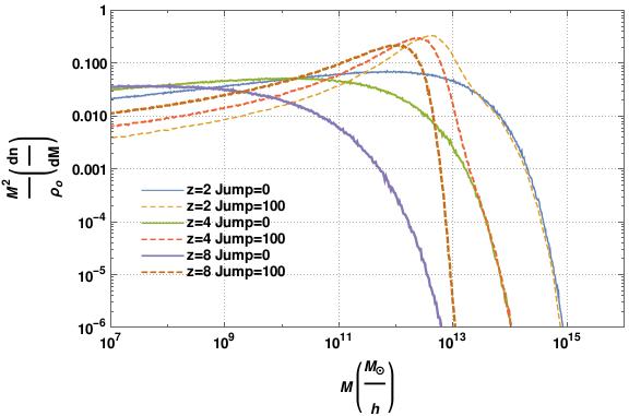
For the same parameters used above, Fig. 4 shows the multiplicity function at selected redshifts. Four trends are clear. First, the enhancement in the primordial power spectrum leads to enhancement in the number of halos at intermediate masses, culminating approximately at the mass scale corresponding to the length scale to where the jump in the power spectrum is placed. The second is that the effect is larger, and is apparent for a larger range in masses, at higher redshifts. Indeed, Fig. 5 shows a maximum enhancement of almost four orders of magnitude at , compared to only a factor of a few at . This is because high mass halos are rarer at higher redshifts and thus the relative increase due to the enhancement resulting from the discontinuity in the power spectrum is larger. It also results in the rate of change in the mass function with redshift, at fixed mass, being smaller in the case of enhanced spectrum than in the unperturbed case.
Finally, there is the somewhat counterintuitive effect, mentioned at the conclusion of the previous subsection, of significant suppression of the multiplicity function contribution of halos at smaller masses, below a few . This interesting result may be understood by recalling that enhancement in the power spectrum at comoving scales associated with masses of , implies that all smaller scales are also enhanced. And enhancement at smaller (length and mass) scales in turn implies that smaller halos form at higher redshift and that by the redshifts considered here they have already been typically subsumed in larger ones; that is, the typical mass scale, for a given fluctuation level at a given redshift, shifts up. This leads to a relative decrease in the number of halos with masses . As opposed to the case of the enhancement of the multiplicity of relatively high mass halos, the de-enhancement is here relatively larger at smaller , as the lower mass halos are now those that are rarer at such redshifts.
IV.3 Interpretation and possible consequences
As, in the current model of structure formation, galaxies form in seeds provided by the potential wells of dark matter halos, the significant modifications to the halo mass function are expected to leave imprints on the associated galaxy stellar mass function. Pertinent questions here thus include whether those modifications have consequences for problems arising at small scales within the current standard scenario of structure formation, as outlined in the introduction; or, in contrast, whether such modifications can constrained also on nonlinear scales.
IV.3.1 Small scale problems at low redshift and the dearth of dwarf galaxies
One straightforward consequence of the suppression of halo multiplicity at small scales pertains to the longstanding issue of the dearth of dwarf galaxies in the standard scenario: a galaxy like the Milky Way is expected, in the context of the CDM with a standard primordial power spectrum, to have hundreds of satellites that are not observed, and some of the predicted hosting halos are too ’large’ to have ’failed’ to form galaxies. These are aspects of the so-called small scale problems of the standard scenario has given rise to various explanations, e.g in terms of baryonic physics, warm dark matter, fuzzy dark matter, as well as direct suppression of the small scale power spectrum.
Our somewhat counter-intuitive result, on the other hand, is that an enhancement of power on small scales can also lead to a suppression in the number of small halos (as these ‘overmerge’ into larger entities). This suppression at at the scales where issues such as the dearth of small galaxies () and too big to fail () problems appear, can therefore be of relevance to apparent small scale crises arising in the context the standard model of structure formation. The order of magnitude suppression at smaller masses is directly relevant to resolving the apparent discrepancy between the number of observed small satellite galaxies and large number of small halos found in cold dark matter simulations. The suppression on the larger mass scales, on the other hand, may help alleviate the too big to fail issue; when this is posed as an abundance matching problem, whereby the abundance of simulated halos is too large at the masses inferred from the dynamics of observed galaxies in the range (e.g., ref. Miller et al. 2014).
IV.3.2 The excess of early massive galaxies
The enhancement at higher mass scales may, on the other hand, have consequences for the more recently raised issues associated with early galaxy formation. These are extensions of longstanding phenomena related to what is referred to as ’downsizing’ (e.g. Somerville and Davé 2015), required to account for preponderance of early massive galaxies; a phenomenon that does not appear entirely natural in a hierarchical structure formation scenario, where the smaller halos embodying the potential wells hosting the galaxies form first.
The problem of early galaxy formation has been termed ‘impossibly early’ in the context of the standard CDM scenario of structure formation Steinhardt et al. 2016. In that work, the authors attempt to infer the halo mass function at high-, primarily from stellar mass functions derived using photometric spectral energy distribution templates and ultraviolet luminosity functions. The halo mass is then inferred by assuming a stellar to halo mass of . If this local value of is used, then Fig. 1 of the aforementioned work suggests that the number density of massive galaxies can greatly exceed that of the halos they should inhabit for in the standard CDM structure formation scenario. The discrepancy becomes more severe as one moves up in redshift and mass, reaching four orders of magnitude or more.
The above would seem to rule out the standard scenario of structure formation in the context of CDM cosmology. However, a couple of caveats have been pointed out. First, regarding the assumption that does not vary with redshift. For, as can also be seen from Fig. 1 of Steinhardt et al. 2016, instead of moving the points inferred from the observed stellar number densities down orders of magnitude to fit the corresponding halo number densities, one can move the points horizontally to the left by an order of magnitude. This fitting procedure in effect invokes a (and ) dependent , to replace the fiducial local value of assumed by the authors. The procedure, requiring , is still in principle consistent with a universal baryon fraction of , associated with the standard cosmological scenario, but only just Behroozi and Silk 2018 33 3 Note that in Behroozi and Silk 2018 the more conservative cumulative stellar mass function, which averages over the increasing , is employed. The data for to are consistent with CDM. Tension still arises for the data point shown for at (their Fig. 2 top-left). The results in Fig. 18 of Davidzon et al. 2017 show data consistent with , or even larger, already at , for . In general, it seems that galaxies can be accommodated into halos with for if one keeps to (e.g., Behroozi et al. 2013, and Fig. 9 of Behroozi et al. 2019). On the other hand, the most extreme cases in the data presented by Steinhardt et. al. Steinhardt et al. 2016 (where seems required), are just barely consistent with standard CDM..
Another caveat that has been pointed out concerns the extraction of and associated number densities from the ultraviolet luminosity function at high , which some of the data points of Steinhardt et al. 2016 relies on Mancuso et al. 2016. However, a multi-wavelength analysis of a sample of massive galaxies at also leads to a cumulative mass function that can be consistent (within estimated errors) with approaching the universal baryon fraction at and Alcalde Pampliega et al. 2019. That work also shows (Fig. 14) that the number densities of massive galaxies are very difficult to reproduce in hydrodynamic numerical simulations — with significant underestimate for — which may be expected, as their reproduction would seem to require that all available baryons reside inside galaxies, and their near total conversion to stars over a short time (). This would have as consequence the presence of a significantly ‘quenched’, quiescent population of massive galaxies already at high redshift. The presence of such a population, which is indeed observed, poses significant challenges. Synthesizing the stellar populations of one such object, observed at , for example, seems to again require prior evolution involving a reaching the universal baryon fraction Glazebrook et al. 2017b (see also Mawatari et al. 2019). There now appears to be a substantial population of such galaxies, observed at increasing redshift Straatman et al. 2014; Schreiber et al. 2018; Santini et al. 2019; Merlin et al. 2019; Valentino et al. 2020; Girelli et al. 2019; Forrest et al. 2019, and not easily reproduced by either hydrodynamic simulations Merlin et al. 2019; Valentino et al. 2020 or semi analytical models Schreiber et al. 2018; Girelli et al. 2019.
Although questions as to the ultimate severity of these problems will only be settled with the next generation surveys (e.g. with the JWST), the situation warrants pointing out that they can in principle be alleviated by invoking small scale enhancement of the primordial power spectrum examined here.


Fig. 5 shows that significant enhancements can be achieved at mass scales , with a peak at a scale corresponding to highest dark matter to stellar mass ratio in standard modelling, at which the enhancements reach even the ‘impossibly’ large levels claimed in Steinhardt et al. 2016. Perhaps no less important is the slower evolution of the mass function for , observed in Fig. 6, which is more consistent with the redshift evolution of the inferred stellar mass densities in Steinhardt et al. 2016 than the much faster evolution in the standard case (the slow evolution of the stellar mass function for was also observed for example by Song et. al. Song et al. 2016). This would seem to waive the apparent requirement of a that is high dependent on redshift in order to fit the data.
With better statistics, and firmer grip on observational systematics, it should be possible to distinguish between scenarios involving enhancement in the primordial power spectrum, such as the one presented here and reconciliation with data through improvement of the baryonic model; by invoking further ‘downsizing’ physics input, in terms of feedback, quenching and other ‘subgrid’ physics (assuming the data remain consistent with the strict upper bounds placed in the context of CDM Behroozi and Silk 2018). As the baryonic models become better constrained, there may be particular consequences that could also constrain (or confirm) the sort of scenario discussed here. We now discuss some of these.
IV.3.3 Other observables, constraints and variation on basic model


In the context of the enhanced spectrum scenario presented here, the clustering of halos, on mass scales and redshifts where numbers are predicted to be significantly enhanced, may be measurably different from the standard case. This is because the biasing with respect to the matter distribution would be expected to be different (since they would correspondent to less rare density peaks). Combined clustering and abundance matching analysis in the context of a ‘halo model’ (e.g., Peacock 1999), particularly at higher redshifts Harikane et al. 2016, could thus in principle test, and place constraints on, scenarios involving primordial power spectrum enhancements. The galaxy-matter correlation function, entering into calculations of galaxy-galaxy weak lensing signals, should also be different in the present scenario from the standard case. The difference should again be especially significant at higher redshifts, where the abundance of high mass halos is strongly increased, making for a relatively clumpy matter distribution. Tests are also possible at low redshift. particularly as regards to the peak in abundance of Milky Way sized halos, which seems consistent with observations (Section IV.2.2). Some observations on the other hand suggest that the standard model itself may overpredict the halo mass function at scales Leauthaud et al. 2017; further enhancements of the mass function at such scales may be thus constrained.
Another observable that can potentially place immediate constraints on the scenario discussed here is the Lyman- forest. Here, detailed comparison with data involves complex simulations that depend on assumptions regarding the state of the intergalactic medium, which become less robust at nonlinear scales Arinyo-i Prats et al. 2015; Hui et al. 2017. In the nonlinear regime the modifications in the power spectrum are primarily imprinted in the RMS dispersion and the halo mass function, where the complex pattern of enhancement and suppression at different scales and redshifts would contribute to the mass fluctuations probed by one dimensional Lyman- spectra. The large enhancement at higher masses and redshifts may also affect the thermal history of the intergalactic medium. It may therefore be worth investigating if and how such changes affect the standard constraints regarding the power spectrum. Pending such investigation, as the modifications to the linear power spectrum and mass dispersion considered above are large and fall within the region relevant to Lyman- observations, it apt to probe what is to be expected if more modest modifications are made.
In Fig. 7 (left panel) we show the relative change in the mass function for (about an order of magnitude) smaller perturbation in the power spectrum, as well as on scales deeper in the nonlinear regime. As can be seen, in the former case, significant enhancement in the mass function can still occur at the right scale at higher redshift (where halos are exceedingly rare in the standard scenario), so as to alleviate the apparent early galaxy formation problem. The reduction in number of small halos, relevant to the dearth of small galaxies and too big to fail problems at low , is smaller however.
When the modification in the power spectrum is placed on a smaller spatial scales, deeper in the nonlinear regime (Fig. 7, right panel), the decrease in number of small halos at is again significant and relevant to the dearth of dwarf galaxies, but does not cover all the mass range relevant to the too big to fail problem. As may be expected, the enhancement at high redshifts happens at a smaller mass scale (they are also smaller because halos in the standard scenario are already more abundant at such scales). Enhancement at such scales is not directly applicable to the problem of high at and , as discussed in previous subsection. It may nevertheless be relevant at higher redshift, as the progenitors of massive quiescent galaxies were assembled (especially if the star formation rate density does not steeply decline beyond , as suggested by some authors; c.f. ref. Mawatari et al. 2019, particularly the discussion Section 7.3 and references therein). As one further increases the comoving wavenumber associated with the high energy cutoff , this general trend persists. The suppression on small scales at are found to correspond to masses of small halos that are overabundant in CDM up to comoving cutoff , which essentially avoids Lyman- bounds. At larger modification wavenumbers, however, one finds enhancement rather than suppression at mass scales , relevant to the dearth of dwarf galaxies issue. Although enhancing the power spectrum at such smaller spatial scales would not appear to alleviate any of issues regarding galaxy formation discussed here, it could still have consequences for early black hole formation and the epoch of ionization (see also Hirano et al. 2015).

On the other hand, relaxing the assumption of a sudden jump transition leads to suppression and enhancement of halo abundances on larger mass scales, This allows for retaining the advantages of a sudden cutoff at comoving wavenumber , while keeping the mass function at at unchanged, and modifying the power spectrum much more modestly at (cf. Appendix B, Fig. 12). Fig. 8 shows the relative change in the mass function for such a gradual transition in the power spectrum around a characteristic wavenumber of comoving. As can be seen, significant suppression at is again recovered at mass scales of order , relevant to both the dearth of dwarf galaxies and the too big to fail problems. Enhancement at higher also occurs at scales significantly larger than the corresponding sudden jump case (shown on right panel of Fig. 7), which renders the enhancement more directly relevant to early massive galaxy formation issues. The mass function is unmodified at scales at .
Thus, potential resolution of all or some of the galactic and sub-galactic scale issues through modification of the power spectrum, rather than (or in addition to) baryonic physics input, may in principle be tested and constrained through distinctive predictions. This is true in general and is not confined to our particular simple model of a sudden jump; such tests will thus become more relevant if the small scale issues connected to the standard structure formation scenario are confirmed to persist with incoming observations. In the context of the present scenario, such observations can potentially probe imprints (or lack thereof) of high energy cutoff physics on the relevant astrophysical scales, and place constraints on the duration of inflation, as the ratio of the Hubble scale of inflation to the high energy cutoff scale and the number of inflationary e-folds fix the scale at which the matter power spectrum and halo mass function is modified (cf. Section IV.1.2). For the minimal number of e-folds required to solve the horizon problem for example, is required to address the galactic scale issues discussed. Significant power spectrum modification also require (Section III.4). These tests can be stringent; as, given this scale, and the level of excitation determined by the Boguliubov , the predictions of the simplest scenario of sudden jump through a high energy transition scale, are unique in terms of the expected effect on the power spectrum.
V Conclusion
Slow roll inflation predicts a nearly scale invariant spectrum of primordial fluctuations, which is borne out by precise observations of the cosmic microwave background and large scale structure in the universe. Nevertheless, that prediction is not unique, a variety of effects invoking discontinuous or phased evolution between slow rolls, for example, can lead to anomalous ’features’ in the spectrum. Excited states arising from modes crossing a high energy cutoff scale can also lead to significant modifications to the scale free spectrum. Although these are essentially ruled out at the scales where the aforementioned observations are effective, the primordial spectrum is relatively unconstrained on smaller, currently nonlinear scales, where the matter distribution has collapsed into bound self gravitating objects, washing out the primordial signature by largely encoding it in the halo mass function.
On the contrary, at such scales — which span many more octaves of observable structure than the three that are probed in the linear regime — a variety of issues arise in the context of the standard model of structure formation; such as the ’small scale problems’ at low redshift and the apparent problems involving early galaxy and supermassive black hole formation at higher , which can be seen as extension of longstanding phenomena requiring ’downsizing’ in galaxy formation. As these issues arise precisely at the scales where complex baryonic physics comes to play a central role in the standard scenario of structure formation, it was natural that extensive investigation of solutions in these terms have been pursued. However, as these are also the scales where the primordial spectrum of fluctuations is relatively weakly constrained, this aspect, with its effects and consequences, may also warrant further investigation.
Here we considered the effects of excited states arising from the transiting of fluctuation modes through a high energy cutoff scale. As the power spectrum of primordial fluctuations is effectively an adiabatic invariant of inflaton dynamics (Section II.2.2), adiabatic evolution necessarily leaves the nearly scale free spectrum intact. We next considered a simple model of the opposite extreme; of a sudden jump across the transition. The initial conditions for the fluctuations before the jump are well defined, taking the Bunch Davies form, but with propagation speed . An intuitive, simple ’analogue’ model approximated by such a transition corresponds to the case of a gas or lattice where sound waves do not propagate at all below the interparticle distance, then propagate at an anomalous speed in an effective macroscopic approximation, before finally propagating with the standard sound speed and dispersion relation as the wavelength become progressively larger than the interparticle distance.
In this context, the primordial spectrum is invariably enhanced rather than suppressed (whether the initial or is ), for all scales undergoing the transition through the high energy cutoff (Section III). This is accompanied by strong, tightly spaced oscillations in the power spectrum of generic (as opposed to pure de Sitter) models of inflation, where modes exit the horizon at different phases. Numerical calculations suggest that sufficiently non-adiabatic evolution, leading to significant modification of the power spectrum implies an effectively sudden transition for all and for (Appendix A.2). The simple model of sudden jump, and its predictions, are in this range thus generic. We also considered the possibility of a more gradual transition when the aforementioned conditions are not satisfied (Appendix B).
Given the excitation level induced in the inflaton field, and the current comoving scale corresponding to the jump across the high energy cutoff scale during inflation, the predictions of the simple sudden jump models are essentially unique (in terms of its effect on the matter power spectrum, mass variance and the dark matter halo mass function). The level of excitation can be quantified through a Bogoliubov coefficient for scales that undergo the jump, and is easily evaluated in terms of the in and out frequency ratio (or equivalently ratio; Section III.3). If assumed to be within a few orders of magnitude of the Planck scale, the jump scale corresponds to currently nonlinear scales if inflation proceeds for approximately the number of e-folds necessary to solve the horizon problem. In general, the comoving jump scale corresponds to currently nonlinear scales for minimal inflation if , with smaller ratios allowing for larger e-folds (Section IV.1.2). In this context, the nonlinear scales can be modified, while leaving the standard spectrum intact on linear ones.
Backreaction bounds on must be imposed, as ’over-excitation’ of the inflaton would result in radiation domination rather than inflation; these may however still allow for major enhancements of the power spectrum (and oscillations in the generic inflation case). As we discuss in Section III.4, this would be generally the case if . Such enhancements can have observable consequences, confirming or constraining the effect of excitations on structure formation on nonlinear scales. In order to impose modifications on such scales in particular, and still keep the excitations from overwhelming the inflaton vacuum state, one thus requires and . This implies and . A rough estimate of the derivative of the backreaction suggests possible modification of the power spectrum on the largest scales, and may place tight constraints on the comoving scale at which enhancement of the small scale power spectrum can occur (to about a comoving Mpc; Section III.4). That modification on the largest scales can accompany the changes on small, nonlinear ones, is an interesting possibility that may be worth studying in detail.
To probe for possible characteristic signatures of the modifications on nonlinear scales, we evaluate (in Section IV) the dark halo multiplicity function, quantifying the fraction of mass in halos of mass . In our fiducial example, the peak, resulting from power spectrum enhancement, is chosen to correspond to a few times . This is the mass scale where the highest mass to light ratio is inferred when associating galaxies with halos in the context of halo models derived within the standard scenario. It is also the scale where issues related to the apparent preponderance of early massive galaxies, particularly quiescent ones, appear (Section IV.3.2). For relatively small enhancements at small redshifts , the enhancement at larger is dramatic, as such massive halos are very rare at these redshifts in the standard scenario. The change in the number densities of massive galaxy-hosting halos with redshift is also much smaller than in the standard case. Combined, these effects may alleviate the apparent ’impossibly’ early galaxy formation problem, even in the most extreme form claimed.
Perhaps more surprisingly, an enhancement of the spectrum at these intermediate nonlinear scales leads to suppression of small halos at low , thus potentially alleviating longstanding issues related to the dearth of small galaxies, including those ’too big to fail’, in the standard structure formation scenario. This is due to the enhanced spectrum leading to overmerging of small mass objects at high , so as to lead to a suppression of such objects at low .
The halo mass function, in itself, cannot place strong constraints on enhancements of the primordial power spectrum on currently nonlinear scales, as one can vary the galaxy halo occupation number to match the data (in the standard scenario, the early galaxy formation issues at high and arises because this seems to sometimes require very large stellar mass fraction, which the enhanced halo mass function here may resolve; Section IV.3.2 ). However, combined abundance matching and dynamical analysis at low- can. Halo abundance enhancement at the scales considered here appears consistent with such analyses; it may in fact alleviate the apparent overprediction of stellar masses for given dynamical mass for galaxies with stellar mass (Macciò et al. 2020;Section IV.2.2).
Major modifications in the spectrum of primordial fluctuation are eventually encoded in more minor modifications to the nonlinear matter power spectrum, as these enter primarily through the modified halo mass function rather than the statistics of the spatial distribution. Nevertheless, the scenario of an enhanced primordial power spectrum at scales corresponding to currently nonlinear ones, can also be tested through its signature on halo biasing. The fact that more massive halos would be less rare may be expected to particularly impact such observables as galaxy-mass correlations and leasing signals (especially at higher redshift where the effects of enhancement at higher mass scales are more prominent). To address both aforementioned issues — of massive high- massive galaxies and small local ones — simultaneously in the most severe forms claimed, through sudden transitions, also entails significant modifications at scales probed by Lyman- observations (the required modifications are more modest, or at scales that may be less constrained, if only partial resolution of both issues is sought or if the assumption of sudden transition is relaxed; Section IV.3.3).
Thus, observations, coupled with modelling and simulations with modified spectrum, may place constraints on scenarios invoking enhanced power on currently nonlinear scales, distinguishing them from baryonic solutions to the same problems. In the context of the analytical sudden step model primarily considered here, this includes constraints on , , , and the number of inflationary e-folds, as discussed above. Given the field excitation levels (i.e.) and the comoving scale of the high energy transition, the consequences for the matter spectrum and halo mass function are essentially unique. Variants that could also be tested include those involving phased or discontinuous stages of inflation with relatively localized peaks in the primordial spectrum. This will become perhaps more pressing if next generation surveys (e.g. employing the JWST) confirm problems related to early galaxy formation. On smaller (sub-galactic) scales still, primordial power spectrum enhancement may be relevant to early supermassive black hole formation, and the formation of the first dark matter objects, and may be tested through such effects as CMB spectral distortions.
Acknowledgements.
We wish to thank Adel Awad, Alexey Golovnev, Sergio E. Joras, Giovanni Marozzi, Jerome Martin and Joe Silk for useful discussions, and the referee for constructive comments and suggestions. This project was supported financially by the Science and Technology Development Fund (STDF), Egypt. Grant No. 25859.Appendix A Comparison of simplified model with numerical solution, and the effect of relaxing the sudden jump condition
In this appendix we test the approximation of the simplified model of Section II.3, introduced to evaluate the effect of non-adiabatic transition at a high energy cutoff scale on the primordial power spectrum. There are two approximations that were invoked; the sudden step and the neglect the term proportional to in the Mukhanov-Sasaki equations (2) and (7). We start by examining the latter, then we discuss the former.
A.1 Model versus numerical solution of Mukhanov-Sasaki equation with step


We evolve the dynamics of fluctuation modes numerically, using the MS equation (2) for de Sitter and power law inflationary backgrounds, while replacing the term with
| (63) |
where
| (64) |
and is the Heaviside step function. The parameter quantifies the size of the step. such that the sound speed past the step given by ; it can be positive or negative, corresponding to an upward and downward jump in sound speed respectively. As discussed in Section III, in the context of the sudden step scenario they are equivalent in terms of the effect on the power spectrum.
The primordial spectra are evaluated, for both the analytical model and numerical calculations, as described in Section II.3.1. The results are shown and compared in figures 9 and 10, for the case of de Sitter and power law inflation respectively. As noted in Section II.3.1, in the de Sitter case all modes exit the horizon at exactly the same phase. And any initial shift in phase, due to change in effective frequency related to the second term in bracket of the MS equation, leads to corresponding constant difference in the final power spectrum. This leads to a difference between the numerical and analytical results, where the aforementioned term is neglected. Nevertheless, the relative error in the ratio of the perturbed to unperturbed power spectrum is still of order when the step frequency ratio is . It is an order of magnitude lower still when the change of frequency is hundred folds.
In the case of power law inflation the Hubble scale is not exactly constant. The modes exit the horizon at different phases, and this leads to the oscillations, which accompany the enhancement in Fig. 10. The corresponding error is then primarily in phases, with the maxima and minima of the oscillations practically equal in the simplified model and the numerical calculations. The change in phase is generally unimportant for calculating quantities with observable consequences; such as the mass fluctuations at a given spatial or mass scale, and halo mass multiplicity function. For these depend on integrals of the matter power spectrum (as discussed in Section IV). The simple analytical model — with its simple interpretation in terms of well defined in and out states; Section III — thus turns out to be a good approximation.


A.2 Non-adiabaticity versus sudden jump condition
Oscillations can, in general, be considered adiabatic if changes only slightly over a characteristic time of order of one oscillation period. If the frequency changes from a value to another value , on a characteristic timescale , the change may thus be adiabatic if
| (65) |
In the context of our sudden step model, and will correspond to and , respectively. We take the ’typical’ on the right hand side to correspond to the minimal frequency; supposing that the dynamics may be affected non-adibaticaly if the change in frequency is larger than this. To examine to what extent that model may describe a more general situation, where change may be more gradual, we use the logistic function to parametrize the transition:
| (66) |
Here the parameter describes the stiffness of the transition, this being steep and steplike for , and (which may be positive or negative) the scale of the step in the transition. Thus, in the high energy regime limit, the sound speed , while when the transition to the standard low-energy physics regime is complete. In these terms, the characteristic time over which changes between its initial and final value is . The adiabaticity violation condition can then be written as
| (67) |
where we have used , and corresponds to the high energy limit sound speed. Since, as we have seen in Section II.2.2, the power spectrum is essentially an adiabatic invariant of the dynamics of inflationary perturbations, it is necessary to satisfy this condition in order to modify the standard power spectrum.
Two cases are of particular interest in the context of the present study: , so that and , when . For sound speeds considered here, the adiaticity condition (67) is violated at smallest possible when the sound speed is minimal, that is . Still, even in this case, is of order one or larger if , as required to keep the significant changes in power spectrum in the nonlinear regime of structure formation (Section IV.1.2). For our parameters, the transition is thus necessarily stiff.


We now show that the transition is stiff even form much smaller , which is a minimal value, in the sense that with smaller values the effect of the second term in brackets of Eq. (7) becomes important at for (see discussion relating to inequality 11). For it turns out that the adiabaticty condition needs to be quite strongly violated for sufficient change in the dynamics significantly affects the power spectrum (that significant changes occurs well beyond the adiabaticity breaking condition is common in dynamical systems Binney and Tremaine 2008). This can be seen from Fig. 11, where we show that large changes only occur when is orders of magnitudes above the value estimated from (67). This is the case for both the and , with the former being stiffer still as expected from (67) 44 4 Note also, in the latter case of , the small bump on the right, visible in the low spectra beyond the cutoff scale. These are due to non-adibaticity at the crossing of the high energy transition at . They are much less prominent for smaller values, used in the rest of this work. They nevertheless represent another potentially interesting effect associated with non-adiabatic evolution. The transition is stiffer still for smaller values of and larger . Thus, for sound speed ratios considered here, our simple model of a sudden jump, and accompanying signature of a sudden break in the power spectrum, appears much more generic than may seem a priory.
Appendix B Modified mass function from non-sudden spectrum enhancements


As we have seen in the previous appendix, the sudden jump transition in the power spectrum at smaller scales is a good approximation for the parameters primarily considered in this paper, namely for initial ; for such values, the sufficient violation of the adiabaticity condition, required for significant modification of the power spectrum, practically implies a sudden transition. Nevertheless, as is already apparent in Fig. 11, for (right hand panel), the sudden jump approximation becomes less accurate as a predictor of significant change at smaller . If one envisages a transition starting at significantly smaller sound speed still, it may then take place more gradually while still imparting a palpable effect on the power spectrum.
We consider potentially observable consequences of this effect by examining a series of progressively steeper transitions. We do this by modifying the primordial power spectrum in a parametric manner, such that
| (68) |
where is the standard, nearly scale invariant, power spectrum of scalar perturbations. The transition function tends to unity as and vanishes as , and is the enhancement factor (it determines the ratio of the asymptotic values of the power spectrum at small and large scales). We have tried several forms for , and the resulting trends were verified to be generic. Here we show results for the following form (also used in Nakama et al. 2017 for the purpose of suppression of the spectrum rather than enhancement):
| (69) |
where determines the steepness of the transition around . In the following we will take to correspond to a comoving scale of . As equations (39 )and (44) show to be about for a sudden step scenario with initial , the requirement that the initial implies (otherwise, in line with the aforementioned considerations, a gradual transition may not have a significant effect on the power spectrum). In what follows we take .
Fig. 12 shows the primordial power spectrum, as well as the dimensionless matter power spectrum calculated using publicly available CLASS code (class-code.net), for several values of . The corresponding multiplicity functions, calculated using (57) and (60), are shown in Fig. 13, where the left hand panel displays results at . For large , those results are similar to the sudden jump case. For the effect is smeared out, with increase at halo masses , which would increase tension with cluster counts, which is already present in thee standard model. The suppression at small mass scales is enhanced by the gradual transition.
Of particular interest is the intermediate, , case. The enhancement takes place at larger masses than the corresponding case with sudden jump (at ). The suppression at takes place at larger masses as well. This allows for largely retaining the advantages of the sharp cutoff at — in terms of simultaneously alleviating both the dearth of dearth of dwarf galaxy and too big to fail problems at , as well as accounting for early galaxy formation at higher redshifts — while avoiding any enhancement at scales of order at , and relatively mildly perturbing the matter power spectrum at (Fig. 12; see also Section IV.3.3). The enhancement of the mass function at may also be relevant for explaining the overestimation of abundance matching within the standard model of stellar masses of massive galaxies (Macciò et al. 2020; Section IV.2.2).
References
- Lyth and Liddle (2009) D. H. Lyth and A. R. Liddle, The primordial density perturbation: cosmology, inflation and the origin of structure; rev. version (Cambridge Univ. Press, Cambridge, 2009).
- Peter and Uzan (2009) P. Peter and J.-P. Uzan, Primordial cosmology, Oxford Graduate Texts (Oxford Univ. Press, Oxford, 2009).
- Planck Collaboration et al. (2018) Planck Collaboration, Y. Akrami, et al., arXiv e-prints , arXiv:1807.06211 (2018), arXiv:1807.06211 [astro-ph.CO] .
- Salopek et al. (1989) D. S. Salopek, J. R. Bond, and J. M. Bardeen, Phys. Rev. D40, 1753 (1989).
- Dodelson and Stewart (2002) S. Dodelson and E. Stewart, Phys. Rev. D65, 101301 (2002), arXiv:astro-ph/0109354 [astro-ph] .
- Adams et al. (1997) J. A. Adams, G. G. Ross, and S. Sarkar, Physics Letters B 391, 271 (1997), arXiv:hep-ph/9608336 [hep-ph] .
- Chung et al. (2000) D. J. H. Chung, E. W. Kolb, A. Riotto, and I. I. Tkachev, Phys. Rev. D62, 043508 (2000), arXiv:hep-ph/9910437 [hep-ph] .
- Burgess et al. (2003) C. P. Burgess, J. M. Cline, F. Lemieux, and R. Holman, JHEP 02, 048, arXiv:hep-th/0210233 [hep-th] .
- Romano and Sasaki (2008) A. E. Romano and M. Sasaki, Phys. Rev. D78, 103522 (2008), arXiv:0809.5142 [gr-qc] .
- Lyth and Riotto (1999) D. H. D. H. Lyth and A. A. Riotto, Phys. Rep. 314, 1 (1999), arXiv:hep-ph/9807278 [hep-ph] .
- Yamaguchi (2011) M. Yamaguchi, Classical and Quantum Gravity 28, 103001 (2011), arXiv:1101.2488 [astro-ph.CO] .
- Baumann and McAllister (2015) D. Baumann and L. McAllister, Inflation and String Theory (2015).
- Starobinskij (1992) A. A. Starobinskij, Soviet Journal of Experimental and Theoretical Physics Letters 55, 489 (1992).
- Polarski and Starobinsky (1992) D. Polarski and A. A. Starobinsky, Nuclear Physics B 385, 623 (1992).
- Adams et al. (2001) J. Adams, B. Cresswell, and R. Easther, Phys. Rev. D 64, 123514 (2001), arXiv:astro-ph/0102236 [astro-ph] .
- Lesgourgues (2000) J. Lesgourgues, Nucl. Phys. B582, 593 (2000), arXiv:hep-ph/9911447 [hep-ph] .
- Yamaguchi (2001a) M. Yamaguchi, Phys. Rev. D64, 063502 (2001a), arXiv:hep-ph/0103045 [hep-ph] .
- Feng et al. (2003) B. Feng, M.-z. Li, R.-J. Zhang, and X.-m. Zhang, Phys. Rev. D68, 103511 (2003), arXiv:astro-ph/0302479 [astro-ph] .
- Elgaroy et al. (2003) O. Elgaroy, S. Hannestad, and T. Haugboelle, J. Cosmol. Astropart. Phys. 0309, 008, arXiv:astro-ph/0306229 [astro-ph] .
- Gong (2005) J.-O. Gong, J. Cosmol. Astropart. Phys. 0507, 015, arXiv:astro-ph/0504383 [astro-ph] .
- Dvorkin and Hu (2010) C. Dvorkin and W. Hu, Phys. Rev. D81, 023518 (2010), arXiv:0910.2237 [astro-ph.CO] .
- Namjoo et al. (2012) M. H. Namjoo, H. Firouzjahi, and M. Sasaki, J. Cosmol. Astropart. Phys. 1212, 018, arXiv:1207.3638 [hep-th] .
- Lesgourgues et al. (1998) J. Lesgourgues, D. Polarski, and A. A. Starobinsky, Mon. Not. R. Ast. Soc. 297, 769 (1998), arXiv:astro-ph/9711139 [astro-ph] .
- Gramann and Hütsi (2000) M. Gramann and G. Hütsi, Mon. Not. R. Ast. Soc. 316, 631 (2000), arXiv:astro-ph/0003455 [astro-ph] .
- Gramann and Hütsi (2001) M. Gramann and G. Hütsi, Mon. Not. R. Ast. Soc. 327, 538 (2001), arXiv:astro-ph/0102466 [astro-ph] .
- Contaldi et al. (2003) C. R. Contaldi, M. Peloso, L. Kofman, and A. Linde, J. Cosmol. Astropart. Phys. 2003 (7), 002, arXiv:astro-ph/0303636 [astro-ph] .
- Gong (2005) J.-O. Gong, J. Cosmolog. Astropart. Phys. 2005, 015 (2005), arXiv:astro-ph/0504383 [astro-ph] .
- Sinha and Souradeep (2006) R. Sinha and T. Souradeep, Phys. Rev. D 74, 043518 (2006), arXiv:astro-ph/0511808 [astro-ph] .
- Joy et al. (2009) M. Joy, A. Shafieloo, V. Sahni, and A. A. Starobinsky, J. Cosmol. Astropart. Phys. 2009 (6), 028, arXiv:0807.3334 [astro-ph] .
- Kamionkowski and Liddle (2000) M. Kamionkowski and A. R. Liddle, Phys. Rev. Lett. 84, 4525 (2000), arXiv:astro-ph/9911103 [astro-ph] .
- Yokoyama (2000) J. Yokoyama, Phys. Rev. D 62, 123509 (2000), arXiv:astro-ph/0009127 [astro-ph] .
- Zentner and Bullock (2002) A. R. Zentner and J. S. Bullock, Phys. Rev. D 66, 043003 (2002), arXiv:astro-ph/0205216 [astro-ph] .
- Little et al. (2003) B. Little, A. Knebe, and R. R. Islam, Mon. Not. R. Ast. Soc. 341, 617 (2003), arXiv:astro-ph/0205420 [astro-ph] .
- Enqvist et al. (2019) K. Enqvist, T. Sawala, and T. Takahashi, arXiv e-prints , arXiv:1905.13580 (2019), arXiv:1905.13580 [astro-ph.CO] .
- Berezinsky et al. (2010) V. Berezinsky, V. Dokuchaev, Y. Eroshenko, M. Kachelrieß, and M. A. Solberg, Phys. Rev. D 81, 103529 (2010), arXiv:1002.3444 [astro-ph.CO] .
- Leo et al. (2018) M. Leo, C. M. Baugh, B. Li, and S. Pascoli, J. Cosmol. Astropart. Phys. 1812 (12), 010, arXiv:1807.04980 [astro-ph.CO] .
- Yamaguchi (2001b) M. Yamaguchi, Phys. Rev. D64, 063503 (2001b), arXiv:hep-ph/0105001 [hep-ph] .
- Bringmann et al. (2002) T. Bringmann, C. Kiefer, and D. Polarski, Phys. Rev. D65, 024008 (2002), arXiv:astro-ph/0109404 [astro-ph] .
- Easther and Peiris (2006) R. Easther and H. Peiris, J. Cosmol. Astropart. Phys. 0609, 010, arXiv:astro-ph/0604214 [astro-ph] .
- Bean et al. (2008) R. Bean, X. Chen, G. Hailu, S. H. H. Tye, and J. Xu, J. Cosmol. Astropart. Phys. 0803, 026, arXiv:0802.0491 [hep-th] .
- Nakashima et al. (2011) M. Nakashima, R. Saito, Y. Takamizu, and J. Yokoyama, Progress of Theoretical Physics 125, 1035 (2011), arXiv:1009.4394 [astro-ph.CO] .
- Miranda et al. (2012) V. Miranda, W. Hu, and P. Adshead, Phys. Rev. D86, 063529 (2012), arXiv:1207.2186 [astro-ph.CO] .
- Miranda and Hu (2014) V. Miranda and W. Hu, Phys. Rev. D89, 083529 (2014), arXiv:1312.0946 [astro-ph.CO] .
- Park and Sorbo (2012) M. Park and L. Sorbo, Phys. Rev. D 85, 083520 (2012), arXiv:1201.2903 [astro-ph.CO] .
- Gariazzo et al. (2017) S. Gariazzo, O. Mena, H. Ramírez, and L. Boubekeur, Physics of the Dark Universe 17, 38 (2017), arXiv:1606.00842 [astro-ph.CO] .
- Ballesteros et al. (2019) G. Ballesteros, J. Beltran Jimenez, and M. Pieroni, J. Cosmol. Astropart. Phys. 1906 (06), 016, arXiv:1811.03065 [astro-ph.CO] .
- Martin and Brandenberger (2001a) J. Martin and R. H. Brandenberger, Phys. Rev. D63, 123501 (2001a), arXiv:hep-th/0005209 [hep-th] .
- Brandenberger and Martin (2001) R. H. Brandenberger and J. Martin, Mod. Phys. Lett. A16, 999 (2001), arXiv:astro-ph/0005432 [astro-ph] .
- Easther et al. (2001) R. Easther, B. R. Greene, W. H. Kinney, and G. Shiu, Phys. Rev. D64, 103502 (2001), arXiv:hep-th/0104102 [hep-th] .
- Niemeyer (2001) J. C. Niemeyer, Phys. Rev. D63, 123502 (2001), arXiv:astro-ph/0005533 [astro-ph] .
- Martin and Brandenberger (2003) J. Martin and R. Brandenberger, Phys. Rev. D68, 063513 (2003), arXiv:hep-th/0305161 [hep-th] .
- Easther et al. (2005a) R. Easther, W. H. Kinney, and H. Peiris, J. Cosmol. Astropart. Phys. 0508, 001, arXiv:astro-ph/0505426 [astro-ph] .
- Kempf and Lorenz (2006) A. Kempf and L. Lorenz, Phys. Rev. D74, 103517 (2006), arXiv:gr-qc/0609123 [gr-qc] .
- Brandenberger and Martin (2013) R. H. Brandenberger and J. Martin, Class. Quant. Grav. 30, 113001 (2013), arXiv:1211.6753 [astro-ph.CO] .
- Kaloper et al. (2002) N. Kaloper, M. Kleban, A. E. Lawrence, and S. Shenker, Phys. Rev. D66, 123510 (2002), arXiv:hep-th/0201158 [hep-th] .
- Danielsson (2002) U. H. Danielsson, Phys. Rev. D66, 023511 (2002), arXiv:hep-th/0203198 [hep-th] .
- Easther et al. (2002) R. Easther, B. R. Greene, W. H. Kinney, and G. Shiu, Phys. Rev. D66, 023518 (2002), arXiv:hep-th/0204129 [hep-th] .
- Niemeyer et al. (2002) J. C. Niemeyer, R. Parentani, and D. Campo, Phys. Rev. D66, 083510 (2002), arXiv:hep-th/0206149 [hep-th] .
- Chatwin-Davies et al. (2017) A. Chatwin-Davies, A. Kempf, and R. T. W. Martin, Phys. Rev. Lett. 119, 031301 (2017), arXiv:1612.06445 [gr-qc] .
- Brandenberger and Martin (2002) R. H. Brandenberger and J. Martin, Int. J. Mod. Phys. A17, 3663 (2002), arXiv:hep-th/0202142 [hep-th] .
- Zhu et al. (2016) T. Zhu, A. Wang, K. Kirsten, G. Cleaver, and Q. Sheng, Phys. Rev. D93, 123525 (2016), arXiv:1604.05739 [gr-qc] .
- Ashoorioon et al. (2017) A. Ashoorioon, R. Casadio, G. Geshnizjani, and H. J. Kim, J. Cosmol. Astropart. Phys. 1709 (09), 008, arXiv:1702.06101 [hep-th] .
- Armendariz-Picon and Lim (2003) C. Armendariz-Picon and E. A. Lim, J. Cosmol. Astropart. Phys. 0312, 006, arXiv:hep-th/0303103 [hep-th] .
- Amelino-Camelia (2013) G. Amelino-Camelia, Living Rev. Rel. 16, 5 (2013), arXiv:0806.0339 [gr-qc] .
- Hossenfelder (2013) S. Hossenfelder, Living Rev. Rel. 16, 2 (2013), arXiv:1203.6191 [gr-qc] .
- Unruh (1981) W. G. Unruh, Phys. Rev. Lett. 46, 1351 (1981).
- Unruh (1995) W. G. Unruh, Phys. Rev. D51, 2827 (1995).
- Barcelo et al. (2005) C. Barcelo, S. Liberati, and M. Visser, Living Rev. Rel. 8, 12 (2005), [Living Rev. Rel.14,3(2011)], arXiv:gr-qc/0505065 [gr-qc] .
- Chä and Fischer (2017) S.-Y. Chä and U. R. Fischer, Phys. Rev. Lett. 118, 130404 (2017), [Addendum: Phys. Rev. Lett.118,no.17,179901(2017)], arXiv:1609.06155 [cond-mat.quant-gas] .
- Tanaka (2000) T. Tanaka, arXiv e-prints , astro-ph/0012431 (2000), arXiv:astro-ph/0012431 [astro-ph] .
- Niemeyer and Parentani (2001) J. C. Niemeyer and R. Parentani, Phys. Rev. D64, 101301 (2001), arXiv:astro-ph/0101451 [astro-ph] .
- Starobinsky (2001) A. A. Starobinsky, Pisma Zh. Eksp. Teor. Fiz. 73, 415 (2001), [JETP Lett.73,371(2001)], arXiv:astro-ph/0104043 [astro-ph] .
- Giovannini (2003) M. Giovannini, Class. Quant. Grav. 20, 5455 (2003), arXiv:hep-th/0308066 [hep-th] .
- Porrati (2004) M. Porrati, Phys. Lett. B596, 306 (2004), arXiv:hep-th/0402038 [hep-th] .
- Greene et al. (2005) B. R. Greene, K. Schalm, G. Shiu, and J. P. van der Schaar, J. Cosmol. Astropart. Phys. 0502, 001, arXiv:hep-th/0411217 [hep-th] .
- Brandenberger and Martin (2005) R. H. Brandenberger and J. Martin, Phys. Rev. D71, 023504 (2005), arXiv:hep-th/0410223 [hep-th] .
- Danielsson (2005) U. H. Danielsson, Phys. Rev. D71, 023516 (2005), arXiv:hep-th/0411172 [hep-th] .
- Goldstein and Lowe (2003) K. Goldstein and D. A. Lowe, Phys. Rev. D67, 063502 (2003), arXiv:hep-th/0208167 [hep-th] .
- Easther et al. (2005b) R. Easther, W. H. Kinney, and H. Peiris, J. Cosmol. Astropart. Phys. 0505, 009, arXiv:astro-ph/0412613 [astro-ph] .
- Okamoto and Lim (2004) T. Okamoto and E. A. Lim, Phys. Rev. D69, 083519 (2004), arXiv:astro-ph/0312284 [astro-ph] .
- Martin and Ringeval (2005) J. Martin and C. Ringeval, J. Cosmol. Astropart. Phys. 0501, 007, arXiv:hep-ph/0405249 [hep-ph] .
- Martin and Ringeval (2004) J. Martin and C. Ringeval, Phys. Rev. D69, 127303 (2004), arXiv:astro-ph/0402609 [astro-ph] .
- Chluba et al. (2012a) J. Chluba, A. L. Erickcek, and I. Ben-Dayan, Astrophys. J. 758, 76 (2012a), arXiv:1203.2681 [astro-ph.CO] .
- Chluba et al. (2012b) J. Chluba, R. Khatri, and R. A. Sunyaev, MNRAS 425, 1129 (2012b), arXiv:1202.0057 [astro-ph.CO] .
- Emami and Smoot (2018) R. Emami and G. Smoot, J. Cosmol. Astropart. Phys. 1801 (01), 007, arXiv:1705.09924 [astro-ph.CO] .
- Frenk and White (2012) C. S. Frenk and S. D. M. White, Annalen der Physik 524, 507 (2012), arXiv:1210.0544 [astro-ph.CO] .
- Del Popolo and Le Delliou (2017) A. Del Popolo and M. Le Delliou, Galaxies 5, 17 (2017), arXiv:1606.07790 [astro-ph.CO] .
- Bullock and Boylan-Kolchin (2017) J. S. Bullock and M. Boylan-Kolchin, Annual Review of Astronomy and Astrophysics 55, 343 (2017), arXiv:1707.04256 [astro-ph.CO] .
- De Rosa et al. (2014) G. De Rosa et al., Astrophys. J. 790, 145 (2014), arXiv:1311.3260 [astro-ph.CO] .
- Wu et al. (2015) X.-B. Wu, F. Wang, X. Fan, W. Yi, W. Zuo, F. Bian, L. Jiang, I. D. McGreer, R. Wang, J. Yang, Q. Yang, D. Thompson, and Y. Beletsky, Nature (London) 518, 512 (2015), arXiv:1502.07418 [astro-ph.GA] .
- Watson et al. (2015) D. Watson, L. Christensen, K. K. Knudsen, J. Richard, A. Gallazzi, and M. J. Michałowski, Nature (London) 519, 327 (2015), arXiv:1503.00002 [astro-ph.GA] .
- Hirano et al. (2015) S. Hirano, N. Zhu, N. Yoshida, D. Spergel, and H. W. Yorke, Astrophys. J. 814, 18 (2015), arXiv:1504.05186 [astro-ph.CO] .
- Steinhardt et al. (2016) C. L. Steinhardt, P. Capak, D. Masters, and J. S. Speagle, Astrophys. J. 824, 21 (2016), arXiv:1506.01377 [astro-ph.GA] .
- Valiante et al. (2016) R. Valiante, R. Schneider, M. Volonteri, and K. Omukai, MNRAS 457, 3356 (2016), arXiv:1601.07915 [astro-ph.GA] .
- Stefanon et al. (2017) M. Stefanon, R. J. Bouwens, I. Labbé, A. Muzzin, D. Marchesini, P. Oesch, and V. Gonzalez, Astrophys. J. 843, 36 (2017), arXiv:1611.09354 [astro-ph.GA] .
- Glazebrook et al. (2017a) K. Glazebrook, C. Schreiber, I. Labbé, T. Nanayakkara, G. G. Kacprzak, P. A. Oesch, C. Papovich, L. R. Spitler, C. M. S. Straatman, K.-V. H. Tran, and T. Yuan, Nature (London) 544, 71 (2017a), arXiv:1702.01751 [astro-ph.GA] .
- Venemans et al. (2017) B. P. Venemans, F. Walter, R. Decarli, E. Bañados, C. Carilli, J. M. Winters, K. Schuster, E. da Cunha, X. Fan, E. P. Farina, C. Mazzucchelli, H.-W. Rix, and A. Weiss, Astrophys. J. Lett. 851, L8 (2017), arXiv:1712.01886 [astro-ph.GA] .
- Behroozi and Silk (2018) P. Behroozi and J. Silk, MNRAS 477, 5382 (2018), arXiv:1609.04402 [astro-ph.GA] .
- Tang et al. (2019) J.-J. Tang, T. Goto, Y. Ohyama, C. Jin, C. Done, T.-Y. Lu, T. Hashimoto, E. Kilerci Eser, C.-Y. Chiang, and S. J. Kim, MNRAS 484, 2575 (2019), arXiv:1901.02615 [astro-ph.GA] .
- Cecchi et al. (2019) R. Cecchi, M. Bolzonella, A. Cimatti, and G. Girelli, Astrophys. J. 880, L14 (2019), arXiv:1906.11842 [astro-ph.GA] .
- Smith and Bromm (2019) A. Smith and V. Bromm, arXiv e-prints , arXiv:1904.12890 (2019), arXiv:1904.12890 [astro-ph.GA] .
- Wang et al. (2019) T. Wang et al., Nature 572, 211 (2019), arXiv:1908.02372 [astro-ph.GA] .
- El-Zant et al. (2001) A. El-Zant, I. Shlosman, and Y. Hoffman, Astrophys. Jour. 560, 636 (2001), astro-ph/0103386 .
- El-Zant et al. (2004) A. A. El-Zant, Y. Hoffman, J. Primack, F. Combes, and I. Shlosman, Astrophys. Jour.l 607, L75 (2004), astro-ph/0309412 .
- Romano-Díaz et al. (2008) E. Romano-Díaz, I. Shlosman, Y. Hoffman, and C. Heller, Astrophys. Jour.l 685, L105 (2008), arXiv:0808.0195 .
- Goerdt et al. (2010) T. Goerdt, B. Moore, J. I. Read, and J. Stadel, Astrophys. Jour. 725, 1707 (2010), arXiv:0806.1951 .
- Cole et al. (2011) D. R. Cole, W. Dehnen, and M. I. Wilkinson, Mon. Not. Roy. Ast. Soc. 416, 1118 (2011), arXiv:1105.4050 .
- Inoue and Saitoh (2011) S. Inoue and T. R. Saitoh, Mon. Not. Roy. Ast. Soc. 418, 2527 (2011), arXiv:1108.0906 .
- Laporte and White (2015) C. F. P. Laporte and S. D. M. White, Mon. Not. Roy. Ast. Soc. 451, 1177 (2015), arXiv:1409.1924 [astro-ph.GA] .
- Nipoti and Binney (2015) C. Nipoti and J. Binney, Mon. Not. Roy. Ast. Soc. 446, 1820 (2015), arXiv:1410.6169 .
- Del Popolo et al. (2018) A. Del Popolo, F. Pace, M. Le Delliou, and X. Lee, Phys. Rev. D 98, 063517 (2018), arXiv:1809.10609 .
- Read and Gilmore (2005) J. I. Read and G. Gilmore, Mon. Not. Roy. Ast. Soc. 356, 107 (2005), astro-ph/0409565 .
- Mashchenko et al. (2008) S. Mashchenko, J. Wadsley, and H. M. P. Couchman, Science 319, 174 (2008), arXiv:0711.4803 .
- Peirani et al. (2008) S. Peirani, S. Kay, and J. Silk, Atron. & Astrophys. 479, 123 (2008), astro-ph/0612468 .
- Pontzen and Governato (2012) A. Pontzen and F. Governato, Mon. Not. Roy. Ast. Soc. 421, 3464 (2012), arXiv:1106.0499 .
- Teyssier et al. (2013) R. Teyssier, A. Pontzen, Y. Dubois, and J. I. Read, Mon. Not. Roy. Ast. Soc. 429, 3068 (2013), arXiv:1206.4895 .
- Pontzen and Governato (2014) A. Pontzen and F. Governato, Nature 506, 171 (2014), arXiv:1402.1764 [astro-ph.CO] .
- El-Zant et al. (2016) A. A. El-Zant, J. Freundlich, and F. Combes, Mon. Not. Roy. Astron. Soc. 461, 1745 (2016), arXiv:1603.00526 [astro-ph.GA] .
- Colín et al. (2000) P. Colín, V. Avila-Reese, and O. Valenzuela, Astrophys. Jour. 542, 622 (2000), astro-ph/0004115 .
- Bode et al. (2001) P. Bode, J. P. Ostriker, and N. Turok, Astrophys. Jour. 556, 93 (2001), astro-ph/0010389 .
- Macciò et al. (2012) A. V. Macciò, S. Paduroiu, D. Anderhalden, A. Schneider, and B. Moore, Mon. Not. Roy. Ast. Soc. 424, 1105 (2012), arXiv:1202.1282 .
- Lovell et al. (2014) M. R. Lovell, C. S. Frenk, V. R. Eke, A. Jenkins, L. Gao, and T. Theuns, Mon. Not. Roy. Ast. Soc. 439, 300 (2014), arXiv:1308.1399 .
- El-Zant et al. (2015) A. El-Zant, S. Khalil, and A. Sil, Phys. Rev. D 91, 035030 (2015), arXiv:1308.0836 [hep-ph] .
- Spergel and Steinhardt (2000) D. N. Spergel and P. J. Steinhardt, Physical Review Letters 84, 3760 (2000), astro-ph/9909386 .
- Burkert (2000) A. Burkert, Astrophys. Jour.l 534, L143 (2000), astro-ph/0002409 .
- Kochanek and White (2000) C. S. Kochanek and M. White, Astrophys. Jour. 543, 514 (2000), astro-ph/0003483 .
- Miralda-Escudé (2002) J. Miralda-Escudé, Astrophys. Jour. 564, 60 (2002), astro-ph/0002050 .
- Zavala et al. (2013) J. Zavala, M. Vogelsberger, and M. G. Walker, Mon. Not. Roy. Ast. Soc. 431, L20 (2013), arXiv:1211.6426 [astro-ph.CO] .
- Elbert et al. (2015) O. D. Elbert, J. S. Bullock, S. Garrison-Kimmel, M. Rocha, J. Oñorbe, and A. H. G. Peter, Mon. Not. Roy. Ast. Soc. 453, 29 (2015), arXiv:1412.1477 .
- Goodman (2000) J. Goodman, New Astronomy 5, 103 (2000), astro-ph/0003018 .
- Hu et al. (2000) W. Hu, R. Barkana, and A. Gruzinov, Physical Review Letters 85, 1158 (2000), astro-ph/0003365 .
- Schive et al. (2014) H.-Y. Schive, M.-H. Liao, T.-P. Woo, S.-K. Wong, T. Chiueh, T. Broadhurst, and W.-Y. P. Hwang, Physical Review Letters 113, 261302 (2014), arXiv:1407.7762 .
- Marsh and Silk (2014) D. J. E. Marsh and J. Silk, Mon. Not. Roy. Ast. Soc. 437, 2652 (2014), arXiv:1307.1705 [astro-ph.CO] .
- Hui et al. (2017) L. Hui, J. P. Ostriker, S. Tremaine, and E. Witten, Phys. Rev. D 95, 043541 (2017), arXiv:1610.08297 [astro-ph.CO] .
- Genzel et al. (2011) R. Genzel, S. Newman, T. Jones, N. M. Förster Schreiber, K. Shapiro, S. Genel, S. J. Lilly, A. Renzini, L. J. Tacconi, N. Bouché, A. Burkert, G. Cresci, P. Buschkamp, C. M. Carollo, D. Ceverino, R. Davies, A. Dekel, F. Eisenhauer, E. Hicks, J. Kurk, D. Lutz, C. Mancini, T. Naab, Y. Peng, A. Sternberg, D. Vergani, and G. Zamorani, Astrophys, J. 733, 101 (2011), arXiv:1011.5360 [astro-ph.CO] .
- Cava et al. (2018) A. Cava, D. Schaerer, J. Richard, P. G. Pérez-González, M. Dessauges-Zavadsky, L. Mayer, and V. Tamburello, Nature Astronomy 2, 76 (2018), arXiv:1711.03977 [astro-ph.GA] .
- Mukhanov et al. (1992) V. F. Mukhanov, H. A. Feldman, and R. H. Brandenberger, Physics Reports 215, 203 (1992).
- Armendariz-Picon et al. (1999) C. Armendariz-Picon, T. Damour, and V.-i. Mukhanov, Physics Letters B 458, 209 (1999).
- Garriga and Mukhanov (1999) J. Garriga and V. F. Mukhanov, Physics Letters B 458, 219 (1999).
- Salopek and Bond (1990) D. Salopek and J. Bond, Physical Review D 42, 3936 (1990).
- Martin and Brandenberger (2001b) J. Martin and R. H. Brandenberger, Physical Review D 63, 123501 (2001b).
- Lemoine et al. (2001) M. Lemoine, M. Lubo, J. Martin, and J.-P. Uzan, Physical Review D 65, 023510 (2001).
- Martin and Brandenberger (2002) J. Martin and R. H. Brandenberger, Physical Review D 65, 103514 (2002).
- (144) Indeed, as discussed in Section IV.1.2, in order to get modification of the matter power spectrum and halo mass function at scales of the order of a comoving Mpc, which are of particular interest, one needs , much smaller than , which is the smallest we consider.
- Lucchin and Matarrese (1985) F. Lucchin and S. Matarrese, Physical Review D 32, 1316 (1985).
- Lyth and Stewart (1992) D. H. Lyth and E. D. Stewart, Physics Letters B 274, 168 (1992).
- Arkani-Hamed et al. (1998) N. Arkani-Hamed, S. Dimopoulos, and G. Dvali, Physics Letters B 429, 263 (1998), arXiv:hep-ph/9803315 [hep-ph] .
- Antoniadis et al. (1998) I. Antoniadis, N. Arkani-Hamed, S. Dimopoulos, and G. Dvali, Physics Letters B 436, 257 (1998), arXiv:hep-ph/9804398 [hep-ph] .
- Randall and Sundrum (1999) L. Randall and R. Sundrum, Phys. Rev. Lett. 83, 3370 (1999), arXiv:hep-ph/9905221 [hep-ph] .
- Abel and Santiago (2004) S. Abel and J. Santiago, Journal of Physics G Nuclear Physics 30, R83 (2004), arXiv:hep-ph/0404237 [hep-ph] .
- (151) Cf. Ref Greene et al. 2005. Their more rigorous formulation using effective field theory invokes an ’earliest time’, which is defined as the time the smallest CMB scale leaves the cutoff scale. The earliest time here would correspond to that when the first scales cross the high energy cutoff. In both situations the origin of the time variation of the backreaction lies in the same change in number of excited states in the interval between and .
- Bardeen et al. (1986) J. M. Bardeen, J. R. Bond, N. Kaiser, and A. S. Szalay, Astrophys. J. 304, 15 (1986).
- Lukić et al. (2007) Z. Lukić, K. Heitmann, S. Habib, S. Bashinsky, and P. M. Ricker, The Astrophysical Journal 671, 1160 (2007).
- Boyanovsky et al. (2006) D. Boyanovsky, H. J. de Vega, and N. G. Sanchez, Phys. Rev. D 74, 123006 (2006), arXiv:astro-ph/0607508 [astro-ph] .
- Press and Schechter (1974) W. H. Press and P. Schechter, The Astrophysical Journal 187, 425 (1974).
- Bond et al. (1991) J. Bond, S. Cole, G. Efstathiou, and N. Kaiser, The Astrophysical Journal 379, 440 (1991).
- Sheth et al. (2001) R. K. Sheth, H. J. Mo, and G. Tormen, MNRAS 323, 1 (2001), arXiv:astro-ph/9907024 [astro-ph] .
- Sheth and Tormen (2002) R. K. Sheth and G. Tormen, MNRAS 329, 61 (2002), arXiv:astro-ph/0105113 [astro-ph] .
- Despali et al. (2016) G. Despali, C. Giocoli, R. E. Angulo, G. Tormen, R. K. Sheth, G. Baso, and L. Moscardini, MNRAS 456, 2486 (2016), arXiv:1507.05627 [astro-ph.CO] .
- Comparat et al. (2017) J. Comparat, F. Prada, G. Yepes, and A. Klypin, MNRAS 469, 4157 (2017), arXiv:1702.01628 [astro-ph.CO] .
- Macciò et al. (2020) A. V. Macciò, S. Courteau, N. N. Q. Ouellette, and A. A. Dutton, MNRAS 496, L101 (2020), arXiv:2006.00818 [astro-ph.GA] .
- Miller et al. (2014) S. H. Miller, R. S. Ellis, A. B. Newman, and A. Benson, Astrophys. J. 782, 115 (2014), arXiv:1310.1079 [astro-ph.CO] .
- Somerville and Davé (2015) R. S. Somerville and R. Davé, ARAA 53, 51 (2015), arXiv:1412.2712 [astro-ph.GA] .
- (164) Note that in Behroozi and Silk 2018 the more conservative cumulative stellar mass function, which averages over the increasing , is employed. The data for to are consistent with CDM. Tension still arises for the data point shown for at (their Fig. 2 top-left). The results in Fig. 18 of Davidzon et al. 2017 show data consistent with , or even larger, already at , for . In general, it seems that galaxies can be accommodated into halos with for if one keeps to (e.g., Behroozi et al. 2013, and Fig. 9 of Behroozi et al. 2019). On the other hand, the most extreme cases in the data presented by Steinhardt et. al. Steinhardt et al. 2016 (where seems required), are just barely consistent with standard CDM.
- Mancuso et al. (2016) C. Mancuso, A. Lapi, J. Shi, J. Gonzalez-Nuevo, R. Aversa, and L. Danese, Astrophys. J. 823, 128 (2016), arXiv:1604.02507 [astro-ph.GA] .
- Alcalde Pampliega et al. (2019) B. Alcalde Pampliega, P. G. Pérez-González, G. Barro, H. Domínguez Sánchez, M. C. Eliche-Moral, N. Cardiel, A. Hernán-Caballero, L. Rodriguez-Muñoz, P. Sánchez Blázquez, and P. Esquej, Astrophys. Jour. 876, 135 (2019), arXiv:1806.04152 [astro-ph.GA] .
- Glazebrook et al. (2017b) K. Glazebrook, C. Schreiber, I. Labbé, T. Nanayakkara, G. G. Kacprzak, P. A. Oesch, C. Papovich, L. R. Spitler, C. M. S. Straatman, K.-V. H. Tran, and T. Yuan, Nature (London) 544, 71 (2017b), arXiv:1702.01751 [astro-ph.GA] .
- Mawatari et al. (2019) K. Mawatari, A. K. Inoue, T. Hashimoto, J. Silverman, M. Kajisawa, S. Yamanaka, T. Yamada, I. Davidzon, P. Capak, L. Lin, B.-C. Hsieh, Y. Taniguchi, M. Tanaka, Y. Ono, Y. Harikane, Y. Sugahara, S. Fujimoto, and T. Nagao, arXiv e-prints , arXiv:1912.10954 (2019), arXiv:1912.10954 [astro-ph.GA] .
- Straatman et al. (2014) C. M. S. Straatman et al., Astrophys. J. 783, L14 (2014), arXiv:1312.4952 [astro-ph.GA] .
- Schreiber et al. (2018) C. Schreiber, K. Glazebrook, T. Nanayakkara, G. G. Kacprzak, I. Labbé, P. Oesch, T. Yuan, K. V. Tran, C. Papovich, L. Spitler, and C. Straatman, Astron. & Astrophys. 618, A85 (2018), arXiv:1807.02523 [astro-ph.GA] .
- Santini et al. (2019) P. Santini, E. Merlin, A. Fontana, B. Magnelli, D. Paris, M. Castellano, A. Grazian, L. Pentericci, S. Pilo, and M. Torelli, Mon. Not. Roy. Ast. Soc. 486, 560 (2019), arXiv:1902.09548 [astro-ph.GA] .
- Merlin et al. (2019) E. Merlin, F. Fortuni, M. Torelli, P. Santini, M. Castellano, A. Fontana, A. Grazian, L. Pentericci, S. Pilo, and K. B. Schmidt, Mon. Not. Roy. Ast. Soc. 490, 3309 (2019), arXiv:1909.07996 [astro-ph.GA] .
- Valentino et al. (2020) F. Valentino, M. Tanaka, I. Davidzon, S. Toft, C. Gómez-Guijarro, M. Stockmann, M. Onodera, G. Brammer, D. Ceverino, A. L. Faisst, A. Gallazzi, C. C. Hayward, O. Ilbert, M. Kubo, G. E. Magdis, J. Selsing, R. Shimakawa, M. Sparre, C. Steinhardt, K. Yabe, and J. Zabl, Astrophys. J. 889, 93 (2020), arXiv:1909.10540 [astro-ph.GA] .
- Girelli et al. (2019) G. Girelli, M. Bolzonella, and A. Cimatti, arXiv e-prints , arXiv:1910.07544 (2019), arXiv:1910.07544 [astro-ph.GA] .
- Forrest et al. (2019) B. Forrest et al., arXiv e-prints , arXiv:1910.10158 (2019), arXiv:1910.10158 [astro-ph.GA] .
- Song et al. (2016) M. Song et al., Astrophys. Jour. 825, 5 (2016), arXiv:1507.05636 [astro-ph.GA] .
- Peacock (1999) J. A. Peacock, Cosmological Physics, by John A. Peacock, pp. 704. ISBN 052141072X. Cambridge, UK: Cambridge University Press, January 1999. (1999) p. 704.
- Harikane et al. (2016) Y. Harikane et al., Astrophys. J. 821, 123 (2016), arXiv:1511.07873 [astro-ph.GA] .
- Leauthaud et al. (2017) A. Leauthaud, S. Saito, S. Hilbert, A. Barreira, S. More, M. White, S. Alam, P. Behroozi, K. Bundy, J. Coupon, T. Erben, C. Heymans, H. Hildebrandt, R. Mandelbaum, L. Miller, B. Moraes, M. E. S. Pereira, S. A. Rodríguez-Torres, F. Schmidt, H.-Y. Shan, M. Viel, and F. Villaescusa-Navarro, MNRAS 467, 3024 (2017), arXiv:1611.08606 [astro-ph.CO] .
- Arinyo-i Prats et al. (2015) A. Arinyo-i Prats, J. Miralda-Escudé, M. Viel, and R. Cen, J. Cosmol. Astropart. Phys. 1512 (12), 017, arXiv:1506.04519 [astro-ph.CO] .
- Binney and Tremaine (2008) J. Binney and S. Tremaine, Galactic Dynamics: Second Edition, by James Binney and Scott Tremaine. ISBN 978-0-691-13026-2 (HB). Published by Princeton University Press, Princeton, NJ USA, 2008. (Princeton University Press, 2008).
- (182) Note also, in the latter case of , the small bump on the right, visible in the low spectra beyond the cutoff scale. These are due to non-adibaticity at the crossing of the high energy transition at . They are much less prominent for smaller values, used in the rest of this work. They nevertheless represent another potentially interesting effect associated with non-adiabatic evolution.
- Nakama et al. (2017) T. Nakama, J. Chluba, and M. Kamionkowski, Phys. Rev. D 95, 121302 (2017), arXiv:1703.10559 [astro-ph.CO] .
- Davidzon et al. (2017) I. Davidzon et al., Astron. Astrophys. 605, A70 (2017), arXiv:1701.02734 [astro-ph.GA] .
- Behroozi et al. (2013) P. S. Behroozi, R. H. Wechsler, and C. Conroy, Astrophys. Jour. 770, 57 (2013), arXiv:1207.6105 [astro-ph.CO] .
- Behroozi et al. (2019) P. Behroozi, R. H. Wechsler, A. P. Hearin, and C. Conroy, Mon. Not. Roy. Astron. Soc. 488, 3143 (2019), arXiv:1806.07893 .