Wave scattering in frequency domain

Chapter 0 Introduction

Analysis of wave scattering will start from a propagation equation (1) in frequency domain. The equation can be derived from any fundamental equation, e.g. Maxwell equations, Shrödinger equation or Newton equation of motion. Chapter 1, 2 and 3 define analytical formulas for coordinates, modes and S-matrix. Chapter 4 focuses on roughness scattering by using the formulas. Chapter 5, 6 and 7 give us discrete formulation for numerical calculation. Appendix 8, 9, 10, 11, 12, 13, 14, 15 and 16 show detailed derivations of the formulas. The following section 1 shows notation for the SMatrAn formulas before explaining details of the formulas.

1 Notation for the formulas

The report consists of many formulas. This section will show notation for the formulas.

1.

Three dimensional coordinates are represented as $\left(x,y,z\right)$ or $\left(x_{0},x_{1},x_{2}\right)$ , because cyclic permutation of the latter is directly related to modulo 3 operation. The report will also use $\left(r_{0},r_{1},r_{2}\right)$ or $\left(u_{0},u_{1},u_{2}\right)$ . The $z$ , $x_{2}$ , $r_{2}$ or $u_{2}$ is propagating axis. The report chooses the above simpler notation in order to avoid mistakes in operating and programming physical models, and it will never use the general notation $\left(x_{1},x_{2},x_{3}\right)$ .
2.

Partial derivative by $u_{\nu}$ is represented as $\partial/\partial u_{\nu}$ or $\partial_{u\nu}$ . Derivative of function is sometimes noted as “ ${\,}{}^{{}^{\prime}}$ ”.
3.

The report frequently uses matrix and vector notation, and it does not distinguish between the notations. Matrix and column vector are represented by bold symbol fonts as $\boldsymbol{A}$ for example. Especially, $\boldsymbol{\Phi}_{n}$ means column vector of the $n$ -th mode. Transpose and Hermite operators are notated as “ $\,{}^{\mathrm{T}}\,$ ” and “ $\,{}^{\dagger}\,$ ”, respectively. The “ $\,{}^{*}\,$ ” means complex conjugate, and then ${{\boldsymbol{A}}^{\mathrm{T}}}^{\dagger}={\boldsymbol{A}}^{*}$ . Inner product $\boldsymbol{k}{\cdot}\boldsymbol{r}$ is also represented as $\boldsymbol{k}^{\mathrm{T}}\boldsymbol{r}$ , where $\boldsymbol{k}$ and $\boldsymbol{r}$ are wavenumber vector and position vector, respectively.
4.

“ $\left(\partial/\partial x\right)^{\dagger}$ ” means differential operator to the left side as $\boldsymbol{f}^{\dagger}\left(\partial/\partial x\right)^{\dagger}\boldsymbol{g}=\left(\partial\boldsymbol{f}/\partial x\right)^{\dagger}\boldsymbol{g}$ . Integration by parts gives us a relation: $\left(\partial/\partial x\right)^{\dagger}=-\partial/\partial x$ when $\boldsymbol{f}^{\dagger}\boldsymbol{g}$ satisfies a periodic boundary condition.
5.

Dual basis of $\boldsymbol{\Phi}_{n}$ is represented as $\widetilde{\boldsymbol{\Phi}}_{n}$ . The product $\boldsymbol{\Phi}_{m}^{\dagger}\widetilde{\boldsymbol{\Phi}}_{n}$ includes integral for cross section. We will not explicitly show $\iint du_{0}du_{1}$ .
6.

Imaginary unit is denoted as “ $\,i\,$ ”. The “ $\,j\,$ ” will be only used as integer parameter, and “ $\,l\,$ ”, “ $\,m\,$ ”, “ $\,n\,$ ” and their capital letters are also integer. As an exception, the “ $\,L_{\mathrm{s}}$ ” has a special meaning for system length, e.g. scattering region along the $u_{2}$ -axis is defined as $-L_{\mathrm{s}}/2<u_{2}<+L_{\mathrm{s}}/2$ . The “ $\,L_{\mathrm{c}}$ ” means correlation length for other exception. The modulo operation is used only for non-negative integer in order to avoid confusion caused by several definitions, and it is represented as “ $\,\mathrm{mod}\,$ ” or “ $\,\%\,$ ”. A notation “ $\,\%3\,$ ” is frequently omitted in the modulo 3 operation.
7.

Plane wave is defined as $\exp\left(i\boldsymbol{k}^{\mathrm{T}}\boldsymbol{r}-i\omega t\right)$ , where $\omega$ and $t$ are angular frequency and time, respectively. The definition is well known in physics as eq. (34) in Chapter 1 of [1] and in other scientific society [2]. However it is different from the manner of engineering [3, 4]. If you usually use $\exp\left(j\omega t-j\boldsymbol{k}^{\mathrm{T}}\boldsymbol{r}\right)$ as the plane wave, the “ $\,j\,$ ” has to be replaced to “ $\,-i\,$ ” in the report. $\beta_{n}$ is also used as a propagation constant of the $n$ -th mode instead of wavenumber “ $\,k\,$ .”
8.

Fourier-transform (FT) of $f\left(z\right)$ is defined as $\widehat{f}\left(k\right)=\int^{\infty}_{-\infty}f\left(z\right)e^{-ikz}dz$ . The inverse transformation is that $f\left(z\right)=\left(2\pi\right)^{-1}\int^{\infty}_{-\infty}\widehat{f}\left(k\right)e^{ikz}dk$ . Discrete Fourier transform (DFT) is also defined as $\widehat{f}_{\,\mathrm{DFT}}$ in Section 16.G.
9.

The $f\left[l\right]$ represents the discretization of a continuous function $f\left(x\right)$ , which also means an array.
10.

The “ $\,\tilde{\,}\,$ ” and “ $\,\hat{\,}\,$ ”, which are not wide as “ $\,\widetilde{\,}\,$ ” nor “ $\,\widehat{\,}\,$ ”, mean temporary modification of parameters.

[Go to table of contents.] [Go to home.]

Chapter 1 Coordinate transformation for waveguide

This chapter reports coordinate transformation which can be applied to general waveguides. The goal is that we obtain the scale factors after transforming coordinates as shown in Fig. 1.

Refer to caption — Figure 1: Coordinate transfer. The region of $r_{0}$ is at least limited by $r_{0}\kappa_{b}<1$ and $\left|r_{0}\kappa_{w}\right|<1$ .

Let us consider two step transformation for orthogonal curvilinear coordinates such as $\boldsymbol{x}\Rightarrow\boldsymbol{r}\Rightarrow\boldsymbol{u}$ . Considered waveguide is laid on the $x_{2}x_{0}$ -plane, and then $x_{1}\Rightarrow r_{1}\Rightarrow u_{1}$ is identity transformation. We will ignore the $x_{1}$ -axis in the following sections. The $r_{2}$ -axis and the $u_{2}$ -axis are propagation axis, and $\left|r_{2}\right|,\left|u_{2}\right|<L_{\mathrm{s}}/2$ (see section 1). Note that we will introduce two curvatures $\kappa_{b}$ and $\kappa_{w}$ to the transformation, and the region of $r_{0}$ (and $u_{0}$ ) is limited by $\kappa_{b}$ and $\kappa_{w}$ .

1 Two steps of the transformation: $\boldsymbol{x}\Rightarrow\boldsymbol{r}\Rightarrow\boldsymbol{u}$

The first step $\left(x_{0},\,x_{2}\right)\Rightarrow\left(r_{0},\,r_{2}\right)$ is that

\left\{\begin{aligned} x_{2}\left(r_{0},\,r_{2}\right)&=\int^{r_{2}}_{0}f\left(r\right)dr-r_{0}g\left(r_{2}\right),\\ x_{0}\left(r_{0},\,r_{2}\right)&=\int^{r_{2}}_{0}g\left(r\right)dr+r_{0}f\left(r_{2}\right),\\ f\left(r_{2}\right)&=\cos\left(\int^{r_{2}}_{0}\kappa_{b}\left(r\right)dr\right),\\ g\left(r_{2}\right)&=\sin\left(\int^{r_{2}}_{0}\kappa_{b}\left(r\right)dr\right).\end{aligned}\right.

(1)

Section 8.A in Appendix 8 shows details of the above transformation. Equation (1) ensures that the coordinates $\left(r_{0},\,r_{2}\right)$ are orthogonal curvilinear coordinates. Note that $\kappa_{b}\left(r_{2}\right)$ is a signed curvature for waveguide bending as shown in Fig. 1, since eq. (4) gives us the definition of signed curvature:

\kappa_{b}=\left.\frac{\frac{\partial x_{2}}{\partial r_{2}}\frac{\partial^{2}x_{0}}{\partial r_{2}^{2}}-\frac{\partial^{2}x_{2}}{\partial r_{2}^{2}}\frac{\partial x_{0}}{\partial r_{2}}}{\left(\left(\frac{\partial x_{0}}{\partial r_{2}}\right)^{2}+\left(\frac{\partial x_{2}}{\partial r_{2}}\right)^{2}\right)^{3/2}}\right|_{r_{0}=0}\,.

The second step $\left(r_{0},\,r_{2}\right)\Rightarrow\left(u_{0},\,u_{2}\right)$ is defined by

\left\{\begin{aligned} r_{2}\left(u_{0},\,u_{2}\right)&=u_{2}-\int_{0}^{u_{0}}F_{\mathrm{2D}}\left(r_{0}\left(u,\,u_{2}\right),\,r_{2}\left(u,\,u_{2}\right)\right)du\,,\\ r_{0}\left(u_{0},\,u_{2}\right)&=u_{0}\zeta\left(r_{2}\left(u_{0},\,u_{2}\right)\right),\\ F_{\mathrm{2D}}\left(r_{0},\,r_{2}\right)&=\frac{r_{0}\kappa_{w}\left(r_{2}\right)\zeta\left(r_{2}\right)}{\left(1-r_{0}\kappa_{b}\left(r_{2}\right)\right)^{2}+\left(r_{0}\kappa_{w}\left(r_{2}\right)\right)^{2}}\,,\\ \zeta\left(r_{2}\right)&=\exp\left(\int^{r_{2}}_{0}\kappa_{w}\left(r\right)dr\right).\end{aligned}\right.

(2)

Equations (5), (6) and (7) in Section 8.B ensure that the coordinates $\left(u_{0},\,u_{2}\right)$ are orthogonal curvilinear coordinates. Note that $\kappa_{w}\left(r_{2}\left(0,\,u_{2}\right)\right)$ is a signed curvature for waveguide broadening as shown in Fig. 1, since eq. (8) give us the definition of signed curvature:

\kappa_{w}=\left.\frac{\frac{\partial r_{2}}{\partial u_{0}}\frac{\partial^{2}r_{0}}{\partial u_{0}^{2}}-\frac{\partial^{2}r_{2}}{\partial u_{0}^{2}}\frac{\partial r_{0}}{\partial u_{0}}}{\left(\left(\frac{\partial r_{0}}{\partial u_{0}}\right)^{2}+\left(\frac{\partial r_{2}}{\partial u_{0}}\right)^{2}\right)^{3/2}}\right|_{u_{0}=0}\,.

The region of $u_{0}$ must be numerically checked by eqs. (1) and (2) after setting an initial condition:

\left|u_{0}\right|<\min_{-L_{\mathrm{s}}/2<r<L_{\mathrm{s}}/2}\left(\frac{1}{\zeta\left(r\right)\max\left(\left|\kappa_{b}\left(r\right)\right|,\left|\kappa_{w}\left(r\right)\right|\right)}\right)\,.

2 Scale factor

Let us obtain scale factor $h_{0}$ and $h_{2}$ from eqs. (9) and (10) in Section 8.C.

\left\{\begin{aligned} h_{0}&\triangleq\sqrt{\sum_{j=0}^{2}\left(\frac{\partial x_{j}}{\partial u_{0}}\right)^{2}}=\sqrt{\left(\frac{\partial x_{0}}{\partial u_{0}}\right)^{2}+\left(\frac{\partial x_{2}}{\partial u_{0}}\right)^{2}}=\frac{\left(1-r_{0}\kappa_{b}\right)\zeta}{\sqrt{\left(1-r_{0}\kappa_{b}\right)^{2}+\left(r_{0}\kappa_{w}\right)^{2}}}\,,\\ h_{2}&\triangleq\sqrt{\sum_{j=0}^{2}\left(\frac{\partial x_{j}}{\partial u_{2}}\right)^{2}}=\sqrt{\left(\frac{\partial x_{0}}{\partial u_{2}}\right)^{2}+\left(\frac{\partial x_{2}}{\partial u_{2}}\right)^{2}}=\frac{\partial r_{2}}{\partial u_{2}}\sqrt{\left(1-r_{0}\kappa_{b}\right)^{2}+\left(r_{0}\kappa_{w}\right)^{2}}\,.\end{aligned}\right.

(3)

Note that $\kappa_{b}$ , $\kappa_{w}$ and $\zeta$ are functions of $r_{2}$ . The $\partial r_{2}/\partial u_{2}$ for $h_{2}$ can be numerically solved by

\left\{\begin{aligned} \frac{\partial r_{2}\left(u_{0},\,u_{2}\right)}{\partial u_{2}}&=1-\int_{0}^{u_{0}}\left[\frac{\partial}{\partial u_{2}}F_{\mathrm{2D}}\left(r_{0}\left(u,\,u_{2}\right),\,r_{2}\left(u,\,u_{2}\right)\right)\right]du\,,\\ \frac{\partial F_{\mathrm{2D}}\left(r_{0},\,r_{2}\right)}{\partial u_{2}}&=\frac{\partial r_{2}}{\partial u_{2}}\frac{r_{0}\zeta\left[\kappa_{w}^{{}^{\prime}}\left(1-r_{0}\kappa_{b}\right)^{2}+2\kappa_{w}\left(1-r_{0}\kappa_{b}\right)\left(\kappa_{w}+r_{0}\kappa_{b}^{{}^{\prime}}\right)-r_{0}^{2}\kappa_{w}^{2}\kappa_{w}^{{}^{\prime}}\right]}{\left[\left(1-r_{0}\kappa_{b}\right)^{2}+\left(r_{0}\kappa_{w}\right)^{2}\right]^{2}}\,,\end{aligned}\right.

(4)

where $\kappa_{b}^{{}^{\prime}}=d\kappa_{b}/dr_{2}$ and $\kappa_{w}^{{}^{\prime}}=d\kappa_{w}/dr_{2}$ . See eq. (11) for details of $\partial F_{\mathrm{2D}}/\partial u_{2}$ .

When $\left|u_{0}\kappa_{b}\right|,\left|u_{0}\kappa_{w}\right|\ll 1$ and $\left|u_{0}^{2}\kappa_{b}^{{}^{\prime}}\right|,\left|u_{0}^{2}\kappa_{w}^{{}^{\prime}}\right|\ll 1$ , eq. (3) is approximated to

\left\{\begin{aligned} h_{0}&\simeq\zeta\left(u_{2}\right)\,,\\ \mathit{\Delta}h_{2}&\triangleq h_{2}-1\simeq-u_{0}\zeta\kappa_{b}-\frac{u_{0}^{2}}{2}\zeta^{2}\kappa_{w}^{{}^{\prime}}\,.\end{aligned}\right.

(5)

Note that $r_{2}$ can be replaced to $u_{2}$ , since $r_{2}=u_{2}-O\left(u_{0}^{2}\kappa_{w}\right)$ from eq. (2).

When a condition $\zeta\simeq 1$ , i.e. $\left|\kappa_{w}\right|\ll 2/L$ is applied to eq. (5), $h_{0}$ and $h_{2}$ are furthermore approximated to

\left\{\begin{aligned} \mathit{\Delta}h_{0}&\triangleq h_{0}-1\simeq\int^{u_{2}}_{0}\kappa_{w}\left(u\right)du\,,\\ \mathit{\Delta}h_{2}&=h_{2}-1\simeq-u_{0}\kappa_{b}-\frac{u_{0}^{2}}{2}\kappa_{w}^{{}^{\prime}}\,.\end{aligned}\right.

(6)

[Go to table of contents.] [Go to home.]

Chapter 2 Propagation equation

Fundamental equations, which are Maxwell equation, Shrödinger equation and Newton equation of motion, can be unified to an equation focused on wave propagation in frequency domain $\omega$ . All analysis in the report derives from the propagation equation.

1 Basic relations from propagation equation

Wave-function $\boldsymbol{\Psi}=\left(\boldsymbol{\psi}_{a}^{\mathrm{T}}\,\boldsymbol{\psi}_{b}^{\mathrm{T}}\right)^{\mathrm{T}}$ as a column vector satisfies the following propagation-equation along propagation axis $u_{2}$ :

\boldsymbol{M}\boldsymbol{\Psi}=-i\frac{\partial}{\partial u_{2}}\left(\begin{array}[]{cc}\boldsymbol{0}&\boldsymbol{1}\\ \boldsymbol{1}&\boldsymbol{0}\end{array}\right)\boldsymbol{\Psi}\,.

(1)

The $2\times 2$ matrix elements in the right hand side are square submatrices. Each submatrix is the same size as continuous (or discretized) fields in 2D cross-section of the modes. The square matrix $\boldsymbol{M}$ does not have $\partial_{2}$ , that is, $\boldsymbol{M}u_{2}=u_{2}\boldsymbol{M}$ . We introduce generalized power-flow $P$ along the $u_{2}$ axis, and conservation of the power flow is derived from eq. (1):

\left\{\begin{aligned} P\left(u_{2}\right)&\triangleq\boldsymbol{\Psi}^{\dagger}\left(u_{2}\right)\left(\begin{array}[]{cc}\boldsymbol{0}&\boldsymbol{1}\\ \boldsymbol{1}&\boldsymbol{0}\end{array}\right)\boldsymbol{\Psi}\left(u_{2}\right)\,,\\ \frac{\partial P}{\partial u_{2}}&=i\boldsymbol{\Psi}^{\dagger}\left(\boldsymbol{M}-\boldsymbol{M}^{\dagger}\right)\boldsymbol{\Psi}\,.\end{aligned}\right.

(2)

The right hand side of the second in eq. (2) means power dissipation or power gain. When $\boldsymbol{M}=\boldsymbol{M}^{\dagger}$ , the system has no power-loss for wave propagation.

We also consider the following eigen-mode equation with replacing $-i\partial_{2}$ to propagation constant $\beta_{n}$ as the $n$ -th eigenvalue for eq. (1).

\displaystyle\boldsymbol{M}\,\boldsymbol{\Phi}_{n}

\displaystyle=

\displaystyle\beta_{n}\left(\begin{array}[]{cc}\boldsymbol{0}&\boldsymbol{1}\\ \boldsymbol{1}&\boldsymbol{0}\end{array}\right)\boldsymbol{\Phi}_{n}\,.

The orthogonality of modes is derived from eq. (1) with $\boldsymbol{M}=\boldsymbol{M}^{\dagger}$ .

\boldsymbol{\Phi}_{m}^{\dagger}\left(\begin{array}[]{cc}\boldsymbol{0}&\boldsymbol{1}\\ \boldsymbol{1}&\boldsymbol{0}\end{array}\right)\boldsymbol{\Phi}_{n}=0\quad\mathrm{for}\quad\beta_{m}^{*}\neq\beta_{n}\,.

(6)

Previous work has already discussed orthogonality relation of propagation modes (see equations (3.2-24) in [3] and (10.120) in [4]). We can set power-flow normalization and mode numbering for real $\beta_{n}$ with satisfying that

\boldsymbol{\Phi}_{n}^{\dagger}\left(\begin{array}[]{cc}\boldsymbol{0}&\boldsymbol{1}\\ \boldsymbol{1}&\boldsymbol{0}\end{array}\right)\boldsymbol{\Phi}_{n}=\frac{n}{\left|n\right|}\quad\mathrm{for}\quad n\neq 0\,.

(7)

The above numbering physically means that power flow for positive (negative) $n$ is always positive (negative). If we happen to have a mode with exactly zero power-flow and real $\beta_{n}$ , we can number the mode as $n=0$ and normalize it as $\boldsymbol{\Phi}_{0}^{\dagger}\boldsymbol{\Phi}_{0}=1$ . There is a maximum number $n_{\max}\triangleq\max\left|n\right|$ for real $\beta_{n}$ . Non-real $\beta_{n}$ is numbered $n\gtrless\pm n_{\max}$ with satisfying $n\mathrm{Im}\beta_{n}>0$ , that is, the $n>n_{\max}$ ( $n<-n_{\max}$ ) means evanescent (divergent) wave along the $u_{2}$ axis. A pair of complex conjugate $\beta_{n}$ is also set as $\beta_{n}=\beta_{-n}^{*}$ , and the pair is normalized as

\boldsymbol{\Phi}_{n}^{\dagger}\left(\begin{array}[]{cc}\boldsymbol{0}&\boldsymbol{1}\\ \boldsymbol{1}&\boldsymbol{0}\end{array}\right)\boldsymbol{\Phi}_{-n}=1\quad\mathrm{for}\quad n\gtrless\pm n_{\max}\,.

(8)

All of $\beta_{n}$ consists of real numbers and/or complex conjugate pairs when $\boldsymbol{M}=\boldsymbol{M}^{\dagger}$ , because a secular equation for generalized eigenvalue problem $\boldsymbol{A}\boldsymbol{X}=\lambda\boldsymbol{B}\boldsymbol{X}$ can be deformed into $\left|\boldsymbol{A}-\lambda\boldsymbol{B}\right|=\left|\boldsymbol{A}^{\dagger}-\lambda^{*}\boldsymbol{B}^{\dagger}\right|=0$ . Note that the numbering of the complex conjugate pairs except for pure imaginary $\beta_{n}$ is different from one of Fig. 10.14 and eq. (10.125) in [4]. Here, we try to define dual basis $\widetilde{\boldsymbol{\Phi}}_{n}$ for the basis $\boldsymbol{\Phi}_{n}$ :

\displaystyle\widetilde{\boldsymbol{\Phi}}_{n}=\begin{cases}\frac{n}{\left|n\right|}\tiny\left(\begin{array}[]{cc}\boldsymbol{0}&\boldsymbol{1}\\ \boldsymbol{1}&\boldsymbol{0}\end{array}\right)\normalsize\boldsymbol{\Phi}_{n}&\mathrm{for}\quad 0<\left|n\right|\leq n_{\max}\,,\\ \tiny\left(\begin{array}[]{cc}\boldsymbol{0}&\boldsymbol{1}\\ \boldsymbol{1}&\boldsymbol{0}\end{array}\right)\normalsize\boldsymbol{\Phi}_{-n}&\mathrm{for}\quad\left|n\right|>n_{\max}\,,\\ \boldsymbol{\Phi}_{0}-\sum_{m\neq 0}\left(\boldsymbol{\Phi}_{m}^{\dagger}\boldsymbol{\Phi}_{0}\right)\widetilde{\boldsymbol{\Phi}}_{m}&\mathrm{for}\quad n=0\,.\end{cases}

(9)

Equation (6) and the above normalization rules give us bi-orthogonality [2, 5] and p. 285 of [6] as

\boldsymbol{\Phi}_{m}^{\dagger}\widetilde{\boldsymbol{\Phi}}_{n}=\widetilde{\boldsymbol{\Phi}}_{m}^{\dagger}\boldsymbol{\Phi}_{n}=\delta_{mn}\,,\quad\mathrm{and}\quad\sum_{n}\boldsymbol{\Phi}_{n}\widetilde{\boldsymbol{\Phi}}_{n}^{\dagger}=1\,.

The $n=0$ will be void below, because practical calculations can avoid it by slightly shifting the frequency $\omega$ .

The mode equation (1) can be extended to periodic system using the $\boldsymbol{M}_{p}$ of eq. (10) in Appendix 9. Note that the representation basis with non-real eigenvalue of the $\boldsymbol{M}_{p}$ have to be redefined to satisfy eq. (7) as shown in eq. (6).

2 Special cases of mode equation

Appendices 10, 11 and 12 show details of eq. (1) for the Shrödinger equation, Maxwell’s equations and Newton’s equation of motion, respectively.

This section focuses on two special cases: Shrödinger equation (1) when $A_{z}=0$ , and Maxwell equation (1) when $\boldsymbol{\varepsilon}$ and $\boldsymbol{\mu}$ are diagonal hermitian and $\boldsymbol{\alpha}=\boldsymbol{\gamma}=0$ . From eqs. (3) and (13), the propagation equation (1) becomes that

\boldsymbol{M}\boldsymbol{\Psi}=\left(\begin{array}[]{cc}\boldsymbol{m}_{aa}&\boldsymbol{0}\\ \boldsymbol{0}&\boldsymbol{m}_{bb}\end{array}\right)\boldsymbol{\Psi}=-i\frac{\partial}{\partial u_{2}}\left(\begin{array}[]{cc}\boldsymbol{0}&\boldsymbol{1}\\ \boldsymbol{1}&\boldsymbol{0}\end{array}\right)\boldsymbol{\Psi}\,.

Then,

\boldsymbol{m}_{aa}\boldsymbol{\psi}_{a}=-i\frac{\partial\boldsymbol{\psi}_{b}}{\partial u_{2}}\,,\quad\boldsymbol{m}_{bb}\boldsymbol{\psi}_{b}=-i\frac{\partial\boldsymbol{\psi}_{a}}{\partial u_{2}}\,.

For eq. (3), $\boldsymbol{m}_{aa}$ and $\boldsymbol{m}_{bb}$ are Hermite matrix and a real number, respectively. For eq. (13), $\boldsymbol{m}_{aa}$ and $\boldsymbol{m}_{bb}$ are real symmetric matrices. The mode equation (1) is also that $\boldsymbol{m}_{aa}\boldsymbol{\phi}_{an}=\beta_{n}\boldsymbol{\phi}_{bn}$ and $\boldsymbol{m}_{bb}\boldsymbol{\phi}_{bn}=\beta_{n}\boldsymbol{\phi}_{an}$ as $\boldsymbol{\Phi}_{n}=\left(\boldsymbol{\phi}_{an}^{\mathrm{T}}\,\boldsymbol{\phi}_{bn}^{\mathrm{T}}\right)^{\mathrm{T}}$ . Therefore, eigenvalue problem for $\beta_{n}$ is solved by

\boldsymbol{m}_{bb}\boldsymbol{m}_{aa}\boldsymbol{\phi}_{an}=\beta_{n}^{2}\boldsymbol{\phi}_{an}\quad\mathrm{or}\quad\boldsymbol{m}_{aa}\boldsymbol{m}_{bb}\boldsymbol{\phi}_{bn}=\beta_{n}^{2}\boldsymbol{\phi}_{bn}\,.

For the special case of Shrödinger equation (3), square of the eigenvalue $\beta_{n}^{2}$ is always real, since $\left(\boldsymbol{m}_{bb}\boldsymbol{m}_{aa}\right)^{\dagger}=\boldsymbol{m}_{aa}\boldsymbol{m}_{bb}=\boldsymbol{m}_{bb}\boldsymbol{m}_{aa}$ . Furthermore, the $\boldsymbol{\Phi}_{n}$ satisfies the simpler orthogonality:

\boldsymbol{\phi}_{am}^{\dagger}\boldsymbol{\phi}_{an}=\boldsymbol{\phi}_{bm}^{\dagger}\boldsymbol{\phi}_{bn}=0\quad\textrm{when}\quad\beta_{m}^{2}\neq\beta_{n}^{2}\,.

(10)

The special case (8) for 2D tight-binding model (4) has the same properties as the above.

For the special case of Maxwell equation (1), properties of the $\boldsymbol{\Phi}_{n}$ are different from them for Shrödinger equation. The $\beta_{n}^{2}$ is real or complex, since $\left(\boldsymbol{m}_{bb}\boldsymbol{m}_{aa}\right)^{\dagger}=\boldsymbol{m}_{aa}\boldsymbol{m}_{bb}\neq\boldsymbol{m}_{bb}\boldsymbol{m}_{aa}$ for eq. (13). The $\boldsymbol{\Phi}_{n}$ does not always satisfy eq. (10).

3 Perfectly matched layer (PML) method

The dominating way for treating unbounded problems in numerical simulation is with the PML method [7]. From eq. (1) with $\zeta=1$ of [8] and eq. (2.7) of [9], equation (1) can be modified to

\left[1+i\tilde{\sigma}_{2}\left(u_{2}\right)\right]\boldsymbol{M}\,e^{i\beta_{n}\int^{u_{2}}\left[1+i\tilde{\sigma}_{2}\left(z\right)\right]dz}\,\boldsymbol{\Phi}_{n}=-i\frac{\partial}{\partial u_{2}}\left(\begin{array}[]{cc}\boldsymbol{0}&\boldsymbol{1}\\ \boldsymbol{1}&\boldsymbol{0}\end{array}\right)\,e^{i\beta_{n}\int^{u_{2}}\left[1+i\tilde{\sigma}_{2}\left(z\right)\right]dz}\,\boldsymbol{\Phi}_{n}\,.

(11)

Note that $n\beta_{n}\tilde{\sigma}_{2}\geq 0$ when $0<\left|n\right|\leq n_{\max}$ . The theoretical reflectance $\left|R_{n}\right|^{2}$ of PML with thickness $d$ and power number $M$ is defined as eq. (3) of [10]: $\left|R_{n}\right|^{2}=\exp\left[-4\left|\beta_{n}d\right|\max\left(\tilde{\sigma}_{2}\right)/\left(M+1\right)\right]$ , where $d\gtrsim 2\lambda_{0}/3$ for vacuum wavelength $\lambda_{0}$ , and $M=2,\,3,\,\mathrm{or}\,4$ [9, 10]. Details of PML formulation for Maxwell’s equations will be shown in eq. (6).

[Go to table of contents.] [Go to home.]

Chapter 3 Non-adiabatic transition in frequency domain

This chapter discusses non-adiabatic transition by using adiabatic picture. Equation (1) is slightly modified to

\left[\boldsymbol{M}^{\left(0\right)}\left(z\right)+\boldsymbol{M}^{\left(1\right)}\left(z\right)\right]\boldsymbol{\Psi}\left(z\right)=-i\frac{\partial}{\partial z}\left(\begin{array}[]{cc}\boldsymbol{0}&\boldsymbol{1}\\ \boldsymbol{1}&\boldsymbol{0}\end{array}\right)\boldsymbol{\Psi}\left(z\right)\,,

(1)

where the $\boldsymbol{M}^{\left(0\right)}$ always satisfies that $\boldsymbol{M}^{\left(0\right)}=\boldsymbol{M}^{\left(0\right)\dagger}$ , but the additional term $\boldsymbol{M}^{\left(1\right)}$ has no limit of Hermitian property. Equation (1) has boundaries at $a$ and $b$ as $-L_{\mathrm{s}}/2\leq a<b\leq L_{\mathrm{s}}/2$ (see section 1). The $\boldsymbol{M}^{\left(0\right)}$ and $\boldsymbol{M}^{\left(1\right)}$ satisfy the following conditions as

\frac{\partial\boldsymbol{M}^{\left(0\right)}}{\partial z}=0\;\;\mathrm{and}\;\;\boldsymbol{M}^{\left(1\right)}=0\quad\mathrm{when}\quad z\leq a\;\;\mathrm{or}\;\;b\leq z\,.

(2)

The eigen-mode equation (1) is rewritten as

\boldsymbol{M}^{\left(0\right)}\left(z\right)\boldsymbol{\Phi}_{m}\left(z\right)=\beta_{m}\left(z\right)\left(\begin{array}[]{cc}\boldsymbol{0}&\boldsymbol{1}\\ \boldsymbol{1}&\boldsymbol{0}\end{array}\right)\boldsymbol{\Phi}_{m}\left(z\right)\,.

1 Adiabatic picture

To discuss the $\boldsymbol{\Psi}\left(z\right)$ in eq. (1), we introduce adiabatic picture:

\boldsymbol{\Psi}_{m}^{\left(0\right)}\left(z\right)\triangleq\exp\left(i\int_{0}^{z}\beta_{m}\left(u\right)du\right)\boldsymbol{\Phi}_{m}\left(z\right)\quad\mathrm{and}\quad\widetilde{\boldsymbol{\Psi}}_{m}^{\left(0\right)\dagger}\left(z\right)\triangleq\widetilde{\boldsymbol{\Phi}}_{m}^{\dagger}\left(z\right)\exp\left(-i\int_{0}^{z}\beta_{m}\left(u\right)du\right)\,,

(3)

where eqs. (9) and (3) give us

\widetilde{\boldsymbol{\Psi}}_{m}^{\left(0\right)\dagger}\left(z\right)\boldsymbol{\Psi}_{n}^{\left(0\right)}\left(z\right)=\delta_{mn}\quad\mathrm{and}\quad\sum_{m\neq 0}\boldsymbol{\Psi}_{m}^{\left(0\right)}\left(z\right)\widetilde{\boldsymbol{\Psi}}_{m}^{\left(0\right)\dagger}\left(z\right)=1\,.

(4)

The $\widetilde{\boldsymbol{\Psi}}_{m}^{\left(0\right)\dagger}\left(z\right)$ and $\boldsymbol{\Psi}_{m}^{\left(0\right)}\left(z\right)$ can also represent $\left\langle\widetilde{\boldsymbol{\Psi}}_{m}^{\left(0\right)}\left(z\right)\right|$ and $\left|\boldsymbol{\Psi}_{m}^{\left(0\right)}\left(z\right)\right\rangle$ using the bra-ket notation, respectively. Equations (3) and (4) describe the operators $\boldsymbol{M}^{\left(0\right)}\left(z\right)$ and $\boldsymbol{M}^{\left(1\right)}\left(z\right)$ in eq. (1) as

\boldsymbol{M}^{\left(0\right)}\left(z\right)=\sum_{m\neq 0}\beta_{m}\left(z\right)\left(\begin{array}[]{cc}\boldsymbol{0}&\boldsymbol{1}\\ \boldsymbol{1}&\boldsymbol{0}\end{array}\right)\boldsymbol{\Psi}_{m}^{\left(0\right)}\left(z\right)\widetilde{\boldsymbol{\Psi}}_{m}^{\left(0\right)\dagger}\left(z\right)\quad\mathrm{and}\quad\boldsymbol{M}^{\left(1\right)}\left(z\right)=\sum_{m,n\neq 0}{M}^{\left(1\right)}_{mn}\boldsymbol{\Psi}_{m}^{\left(0\right)}\left(z\right)\widetilde{\boldsymbol{\Psi}}_{n}^{\left(0\right)\dagger}\left(z\right)\,.

(5)

From eqs. (5) and (3), the $\boldsymbol{\Psi}_{m}^{\left(0\right)}$ satisfies that

\left[\frac{\partial}{\partial z}-i\left(\begin{array}[]{cc}\boldsymbol{0}&\boldsymbol{1}\\ \boldsymbol{1}&\boldsymbol{0}\end{array}\right)\left(\boldsymbol{M}^{\left(0\right)}+\boldsymbol{M}^{\left(1\right)}\right)\right]\boldsymbol{\Psi}_{m}^{\left(0\right)}\left(z\right)=\left[\boldsymbol{D}\left(z\right)-i\left(\begin{array}[]{cc}\boldsymbol{0}&\boldsymbol{1}\\ \boldsymbol{1}&\boldsymbol{0}\end{array}\right)\boldsymbol{M}^{\left(1\right)}\left(z\right)\right]\boldsymbol{\Psi}_{m}^{\left(0\right)}\left(z\right)+\boldsymbol{\Psi}_{m}^{\left(0\right)}\left(z\right)\frac{\partial}{\partial z}\,,

(6)

where

\begin{split}\boldsymbol{D}\left(z\right)&\triangleq\sum_{n\neq 0}\exp\left(i\int_{0}^{z}\beta_{n}\left(u\right)du\right)\frac{\partial\boldsymbol{\Phi}_{n}}{\partial z}\widetilde{\boldsymbol{\Psi}}_{n}^{\left(0\right)\dagger}\left(z\right)=\sum_{m,n\neq 0}\boldsymbol{\Psi}_{m}^{\left(0\right)}\left(z\right)D_{mn}\left(z\right)\widetilde{\boldsymbol{\Psi}}_{n}^{\left(0\right)\dagger}\left(z\right)\,,\\ D_{mn}&=\widetilde{\boldsymbol{\Phi}}_{m}^{\dagger}\left(z\right)\exp\left(-i\int_{0}^{z}\left(\beta_{m}\left(u\right)-\beta_{n}\left(u\right)\right)du\right)\frac{\partial\boldsymbol{\Phi}_{n}}{\partial z}\,.\end{split}

(7)

2 Lippmann-Schwinger equation

We show the following Lippmann-Schwinger equation for the $n$ -th mode with outgoing “ $+$ ” (incoming “ $-$ ”) scattered wave:

\begin{split}\boldsymbol{\Psi}_{n}^{\left(\pm\right)}\left(z\right)&=\boldsymbol{\Psi}_{n}^{\left(0\right)}\left(z\right)+\int_{a}^{b}\boldsymbol{G}_{0}^{\left(\pm\right)}\left(z,\,z^{\prime}\right)\boldsymbol{\hat{M}}\left(z^{\prime}\right)\boldsymbol{\Psi}_{n}^{\left(\pm\right)}\left(z^{\prime}\right)dz^{\prime}\,.\end{split}

(8)

Here we introduce an adiabatic Green operator $\boldsymbol{G}_{0}^{\left(\pm\right)}\left(z,\,z^{\prime}\right)$ to eq. (8):

\boldsymbol{G}_{0}^{\left(\pm\right)}\left(z,\,z^{\prime}\right)\triangleq\pm\sum_{m\neq 0}\boldsymbol{\Psi}_{m}^{\left(0\right)}\left(z\right)\frac{m}{\left|m\right|}H\left(\pm\frac{m}{\left|m\right|}\left(z-z^{\prime}\right)\right)\widetilde{\boldsymbol{\Psi}}_{m}^{\left(0\right)\dagger}\left(z^{\prime}\right)

(9)

with using the Heaviside step function

\begin{cases}H\left(z\right)=1,&z>0\,,\\ H\left(z\right)=0,&z<0\,.\end{cases}

The $\boldsymbol{\hat{M}}$ in eq. (8) is also defined by

\begin{split}\boldsymbol{\hat{M}}\left(z\right)&\triangleq-\boldsymbol{D}\left(z\right)+i\left(\begin{array}[]{cc}\boldsymbol{0}&\boldsymbol{1}\\ \boldsymbol{1}&\boldsymbol{0}\end{array}\right)\boldsymbol{M}^{\left(1\right)}\left(z\right)=\sum_{m,n\neq 0}\boldsymbol{\Psi}_{m}^{\left(0\right)}\left(z\right)\hat{M}_{mn}\left(z\right)\widetilde{\boldsymbol{\Psi}}_{n}^{\left(0\right)\dagger}\left(z\right),\\ \hat{M}_{mn}\left(z\right)&=\widetilde{\boldsymbol{\Psi}}_{m}^{\left(0\right)\dagger}\left(z\right)\left[-\boldsymbol{D}\left(z\right)+i\left(\begin{array}[]{cc}\boldsymbol{0}&\boldsymbol{1}\\ \boldsymbol{1}&\boldsymbol{0}\end{array}\right)\boldsymbol{M}^{\left(1\right)}\left(z\right)\right]\boldsymbol{\Psi}_{n}^{\left(0\right)}\left(z\right).\end{split}

(10)

We can consider outgoing and evanescent (incoming and divergent) scattered-waves to outside by using $\boldsymbol{G}_{0}^{\left(+\right)}$ ( $\boldsymbol{G}_{0}^{\left(-\right)}$ ) of eq. (9), and the $\boldsymbol{G}_{0}^{\left(\pm\right)}$ satisfy that

\left[\frac{\partial}{\partial z}-\boldsymbol{D}\left(z\right)-i\left(\begin{array}[]{cc}\boldsymbol{0}&\boldsymbol{1}\\ \boldsymbol{1}&\boldsymbol{0}\end{array}\right)\boldsymbol{M}^{\left(0\right)}\left(z\right)\right]\boldsymbol{G}_{0}^{\left(\pm\right)}\left(z,\,z^{\prime}\right)=\delta\left(z-z^{\prime}\right).

We can check that eq. (8) satisfies eq. (1) with eqs. (2) by considering eq. (10) and the above equation.

When $\widetilde{\boldsymbol{\Phi}}_{n}^{\dagger}\left(z\right)\partial_{z}\boldsymbol{\Phi}_{n}\left(z\right)=0$ , the $\boldsymbol{\hat{M}}$ in eq. (10) can be also deformed into

\displaystyle\begin{split}\hat{M}_{mn}\left(z\right)&=\widetilde{\boldsymbol{\Psi}}_{m}^{\left(0\right)\dagger}\left(z\right)\left(\begin{array}[]{cc}\boldsymbol{0}&\boldsymbol{1}\\ \boldsymbol{1}&\boldsymbol{0}\end{array}\right)\left[\frac{\left(1-\delta_{mn}\right)\frac{\partial\boldsymbol{M}^{\left(0\right)}}{\partial z}}{\beta_{m}\left(z\right)-\beta_{n}\left(z\right)+0}+i\boldsymbol{M}^{\left(1\right)}\right]\boldsymbol{\Psi}_{n}^{\left(0\right)}\left(z\right)\\ &=\frac{m}{\left|m\right|}\boldsymbol{\Psi}_{m}^{\left(0\right)\dagger}\left(z\right)\left[\frac{\left(1-\delta_{mn}\right)\frac{\partial\boldsymbol{M}^{\left(0\right)}}{\partial z}}{\beta_{m}\left(z\right)-\beta_{n}\left(z\right)+0}+i\boldsymbol{M}^{\left(1\right)}\right]\boldsymbol{\Psi}_{n}^{\left(0\right)}\left(z\right)\quad\mathrm{for}\quad 0<\left|m\right|\leq n_{\max}\left(z\right).\end{split}

(11)

If $\widetilde{\boldsymbol{\Phi}}_{n}^{\dagger}\left(z\right)\left(\partial\boldsymbol{\Phi}_{n}/\partial z\right)=\phi_{n}\left(z\right)\neq 0$ , a renormalization of $\boldsymbol{\Phi}_{n}$ , which $\exp\left(-\int^{z}\phi_{n}du\right)\boldsymbol{\Phi}_{n}\left(z\right)\Rightarrow\boldsymbol{\Phi}_{n}\left(z\right)$ , can always remove the non-zero $\phi_{n}$ from the case with maintaining $\widetilde{\boldsymbol{\Phi}}_{n}^{\dagger}\boldsymbol{\Phi}_{n}=1$ . Here note that the $\phi_{n}$ always satisfies $\phi_{n}+\phi_{n}^{*}=0$ ( $\phi_{n}+\phi_{-n}^{*}=0$ ) when $\left|n\right|\leq n_{\max}$ ( $\left|n\right|>n_{\max}$ ).

3 Dyson equation and T-matrix equation

We can show the Dyson equation for the non-adiabatic transition.

\begin{split}\boldsymbol{G}^{\left(\pm\right)}\left(z_{0},\,z^{\prime}\right)&\triangleq\boldsymbol{G}_{0}^{\left(\pm\right)}\left(z_{0},\,z^{\prime}\right)+\sum_{N=2}^{\infty}\left[\prod_{j=1}^{N-1}\int_{a}^{b}dz_{j}\boldsymbol{G}_{0}^{\left(\pm\right)}\left(z_{j-1},\,z_{j}\right)\boldsymbol{\hat{M}}\left(z_{j}\right)\right]\boldsymbol{G}_{0}^{\left(\pm\right)}\left(z_{N-1},\,z^{\prime}\right)\\ &=\boldsymbol{G}_{0}^{\left(\pm\right)}\left(z_{0},\,z^{\prime}\right)+\int_{a}^{b}dz_{1}\boldsymbol{G}_{0}^{\left(\pm\right)}\left(z_{0},\,z_{1}\right)\boldsymbol{\hat{M}}\left(z_{1}\right)\boldsymbol{G}^{\left(\pm\right)}\left(z_{1},\,z^{\prime}\right)\,.\end{split}

The T-matrix called as the transition matrix can be also introduced into the non-adiabatic transition as

\begin{split}\boldsymbol{T}^{\left(\pm\right)}\left(z_{0}\right)&\triangleq\boldsymbol{\hat{M}}\left(z_{0}\right)\left[\boldsymbol{1}+\sum_{N=1}^{\infty}\prod_{j=1}^{N}\int_{a}^{b}dz_{j}\boldsymbol{G}_{0}^{\left(\pm\right)}\left(z_{j-1},\,z_{j}\right)\boldsymbol{\hat{M}}\left(z_{j}\right)\right]=\boldsymbol{\hat{M}}\left(z_{0}\right)\left[\boldsymbol{1}+\int_{a}^{b}dz_{1}\boldsymbol{G}_{0}^{\left(\pm\right)}\left(z_{0},\,z_{1}\right)\boldsymbol{T}^{\left(\pm\right)}\left(z_{1}\right)\right]\,.\end{split}

(12)

The perturbed Green operator $\boldsymbol{G}^{\left(\pm\right)}$ or the T-matrix $\boldsymbol{T}^{\left(\pm\right)}$ represents eq.(8) as

\begin{split}\boldsymbol{\Psi}_{n}^{\left(\pm\right)}\left(z_{0}\right)-\boldsymbol{\Psi}_{n}^{\left(0\right)}\left(z_{0}\right)&=\sum_{N=1}^{\infty}\left[\prod_{j=1}^{N}\int_{a}^{b}dz_{j}\boldsymbol{G}_{0}^{\left(\pm\right)}\left(z_{j-1},\,z_{j}\right)\boldsymbol{\hat{M}}\left(z_{j}\right)\right]\boldsymbol{\Psi}_{n}^{\left(0\right)}\left(z_{N}\right)\\ &=\int_{a}^{b}dz^{\prime}\boldsymbol{G}^{\left(\pm\right)}\left(z_{0},\,z^{\prime}\right)\boldsymbol{\hat{M}}\left(z^{\prime}\right)\boldsymbol{\Psi}_{n}^{\left(0\right)}\left(z^{\prime}\right)=\int_{a}^{b}dz^{\prime}\boldsymbol{G}_{0}^{\left(\pm\right)}\left(z_{0},\,z^{\prime}\right)\boldsymbol{T}^{\left(\pm\right)}\left(z^{\prime}\right)\boldsymbol{\Psi}_{n}^{\left(0\right)}\left(z^{\prime}\right)\,.\end{split}

(13)

Note that the T-matrix of eq. (12) is different from transfer matrix discussed in Section 9.B.

4 S-matrix and its Born approximation

We define elements of S-matrix which is discussed in Section 9.A:

S_{mn}\triangleq\begin{cases}\widetilde{\boldsymbol{\Psi}}_{m}^{\left(0\right)\dagger}\left(b\right)\boldsymbol{\Psi}_{n}^{\left(+\right)}\left(b\right)=\delta_{mn}+\int^{b}_{a}dz\,T^{\left(+\right)}_{mn}\left(z\right)&\mathrm{for}\;\;m>0\,,\\ \widetilde{\boldsymbol{\Psi}}_{m}^{\left(0\right)\dagger}\left(a\right)\boldsymbol{\Psi}_{n}^{\left(+\right)}\left(a\right)=\delta_{mn}-\int^{b}_{a}dz\,T^{\left(+\right)}_{mn}\left(z\right)&\mathrm{for}\;\;m<0\,.\end{cases}

(14)

The S-matrix shows the outgoing waves scattered in the region: $-L_{\mathrm{s}}/2\leq a<z<b\leq+L_{\mathrm{s}}/2$ . The SMatrAn can numerically create the S-matrix of eq. (14) by directly solving the propagation equation (1).

If we consider the $\boldsymbol{\hat{M}}$ as a small perturbation term, we can apply the Born approximation to eq. (12):

\boldsymbol{T}\left(z\right)=\boldsymbol{\hat{M}}\left(z\right)+O\left(\left\|\boldsymbol{\hat{M}}\right\|^{2}\right).{}

The $\boldsymbol{S}$ of eq. (14) is approximated to

S_{mn}\simeq\begin{cases}\delta_{mn}+\int_{a}^{b}\hat{M}_{mn}\left(z\right)dz&\mathrm{for}\;\;m>0\,,\\ \delta_{mn}-\int_{a}^{b}\hat{M}_{mn}\left(z\right)dz&\mathrm{for}\;\;m<0\,.\end{cases}

(15)

Equations (11) and (15) give us two pictures for wave-scattering. When $\boldsymbol{M}^{\left(1\right)}=0$ ,

\left\|\boldsymbol{S}-\boldsymbol{1}\right\|\propto\left\|\frac{\partial\boldsymbol{M}^{\left(0\right)}}{\partial z}\right\|

which shows non-adiabatic transition in adiabatic structure. When $\partial\boldsymbol{M}^{\left(0\right)}/\partial z=0$ and $\Im\boldsymbol{M}^{\left(1\right)}\neq 0$ ,

\left|S_{nn}\right|^{2}=1-O\left(\left\|i\boldsymbol{M}^{\left(1\right)}\right\|\right)\quad\mathrm{and}\quad\left|S_{mn}\right|^{2}=O\left(\left\|i\boldsymbol{M}^{\left(1\right)}\right\|^{2}\right)\quad\mathrm{for}\quad m\neq n\,.

Then, we can ignore scattered power from weak absorber as compared to absorbed power in it.

The Born approximation of eq. (15) is suit for not only understanding scattering process but also evaluating roughness scattering. The following section shows the roughness scattering in the framework of the Born approximation.

[Go to table of contents.] [Go to home.]

Chapter 4 Roughness scattering

We introduce parameter diagonal matrix $\boldsymbol{V}\left(u_{0},u_{1},u_{2}\right)$ into $\boldsymbol{M}$ in eq. (1), and the $\boldsymbol{V}$ consists of several scalar functions of $u_{0}$ , $u_{1}$ and $u_{2}$ for the media. The $\boldsymbol{M}$ consists of $\partial_{u0}$ , $\partial_{u1}$ and $\boldsymbol{V}$ , and it is linear with $\boldsymbol{V}$ , i.e. $\boldsymbol{M}\left(\eta\boldsymbol{V}\right)=\eta\boldsymbol{M}\left(\boldsymbol{V}\right)$ . We separate the $\boldsymbol{V}$ into adiabatic part $\boldsymbol{V}^{\left(0\right)}$ and non-adiabatic part $\boldsymbol{V}^{\left(1\right)}$ to use eq. (1) as

\boldsymbol{M}^{\left(0\right)}=\boldsymbol{M}\left(\boldsymbol{V}^{\left(0\right)}\right)\quad\mathrm{and}\quad\boldsymbol{M}^{\left(1\right)}=\boldsymbol{M}\left(\boldsymbol{V}^{\left(1\right)}\right).

(1)

1 Edge roughness of straight waveguide

When the $\boldsymbol{M}^{\left(0\right)}\left(u_{2}\right)$ does not depend on $u_{2}$ , $\beta_{n}$ and $\boldsymbol{\Phi}_{n}$ are constant for $u_{2}$ (or $z$ ), and then this case simplifies eq. (11) for $0<\left|m\right|\leq n_{\max}$ into

\hat{M}_{mn}\left(u_{2}\right)=i\frac{m}{\left|m\right|}\boldsymbol{\Psi}_{m}^{\left(0\right)\dagger}\left(u_{2}\right)\boldsymbol{M}^{\left(1\right)}\left(u_{2}\right)\boldsymbol{\Psi}_{n}^{\left(0\right)}\left(u_{2}\right)=i\frac{m}{\left|m\right|}e^{-i\left(\beta_{m}-\beta_{n}\right)u_{2}\,}\boldsymbol{\Phi}_{m}^{\dagger}\boldsymbol{M}^{\left(1\right)}\left(u_{2}\right)\boldsymbol{\Phi}_{n}\,.

Fourier transform (FT) of the above $\boldsymbol{M}^{\left(1\right)}$ can be used as

\int_{-L_{\mathrm{s}}/2}^{L_{\mathrm{s}}/2}\hat{M}_{mn}\left(u_{2}\right)du_{2}=i\frac{m}{\left|m\right|}\boldsymbol{\Phi}_{m}^{\dagger}\left[\int_{-\infty}^{\infty}\boldsymbol{M}^{\left(1\right)}\left(u_{2}\right)e^{-i\left(\beta_{m}-\beta_{n}\right)u_{2}\,}du_{2}\right]\boldsymbol{\Phi}_{n}=i\frac{m}{\left|m\right|}\boldsymbol{\Phi}_{m}^{\dagger}\widehat{\boldsymbol{M}^{\left(1\right)}}\left(\beta_{m}-\beta_{n}\right)\boldsymbol{\Phi}_{n}\,,

(2)

since $\boldsymbol{M}^{\left(1\right)}=0$ for $\left|u_{2}\right|>L_{\mathrm{s}}/2$ . Then equation (15) can be deformed by eqs. (1) and (2):

S_{mn}-\delta_{mn}\simeq i\boldsymbol{\Phi}_{m}^{\dagger}\widehat{\boldsymbol{M}^{\left(1\right)}}\left(\beta_{m}-\beta_{n}\right)\boldsymbol{\Phi}_{n}=i\boldsymbol{\Phi}_{m}^{\dagger}\boldsymbol{M}\left(\widehat{\boldsymbol{V}^{\left(1\right)}}\left(\beta_{m}-\beta_{n}\right)\right)\boldsymbol{\Phi}_{n}\,.

(3)

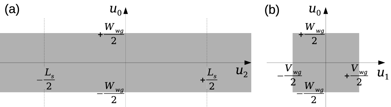
Let us apply eqs. (2) and (3) to wave scattering by waveguide edge roughness. The straight waveguide without roughness has a constant waveguide-width $W_{\mathrm{wg}}$ and a constant waveguide-height $V_{\mathrm{wg}}$ , such as the abrupt case shown in Fig. 1. The $L_{\mathrm{s}}$ means scattering region as mentioned in section 1. This section focuses on roughness by two edges at $u_{0}=\pm W_{\mathrm{wg}}/2$ .

Note that the unperturbed part $\boldsymbol{V}^{\left(0\right)}$ does not depend on $u_{2}$ , and it is function only of $u_{0}$ and $u_{1}$ .

Here, we add two kinds of roughness functions $A_{\mathrm{w}}\left(z\right)$ and $A_{\mathrm{c}}\left(z\right)$ as shown in Fig. 2 to the straight waveguide in Fig. 1.

The $A_{\mathrm{w}}$ and $A_{\mathrm{c}}$ represent line width roughness (LWR) and line center roughness (LCR)[11], respectively. We try to import the roughness functions into the perturbed part $\boldsymbol{V}^{\left(1\right)}$ of eq. (3). There are two approaches of importing the roughness functions.

1 Approach I

The first approach describes the roughness as displacement of waveguide media, and then the $\left(u_{0},u_{1},u_{2}\right)$ coordinates are merely identity transformation of the $\left(x_{0},x_{1},x_{2}\right)$ coordinates, i.e. $h_{j}=1$ for $j=0,1,2$ . The perturbed part $\boldsymbol{V}^{\left(1\right)}$ can be regarded as function of $u_{2}$ via $A_{\mathrm{w}}$ and $A_{\mathrm{c}}$ from Fig. 2:

		$\displaystyle\boldsymbol{V}^{\left(1\right)}\left(A_{\mathrm{w}}\left(u_{2}\right),A_{\mathrm{c}}\left(u_{2}\right)\right)=\boldsymbol{V}^{\left(0\right)}\left(\frac{u_{0}}{1+A_{\mathrm{w}}/W_{\mathrm{wg}}}-A_{\mathrm{c}},u_{1}\right)-\boldsymbol{V}^{\left(0\right)}\left(u_{0},u_{1}\right)$		(4)
		$\displaystyle\simeq\boldsymbol{V}^{\left(0\right)}\left(u_{0}-\frac{u_{0}A_{\mathrm{w}}}{W_{\mathrm{wg}}}-A_{\mathrm{c}},u_{1}\right)-\boldsymbol{V}^{\left(0\right)}\left(u_{0},u_{1}\right)\simeq-\left[\frac{u_{0}A_{\mathrm{w}}\left(u_{2}\right)}{W_{\mathrm{wg}}}+A_{\mathrm{c}}\left(u_{2}\right)\right]\frac{\partial\boldsymbol{V}^{\left(0\right)}\left(u_{0},u_{1}\right)}{\partial u_{0}}$		(4)

when $A_{\mathrm{w}}/2,A_{\mathrm{c}}\ll W/2$ . In the framework of the above formulation (4), the $\widehat{\boldsymbol{V}^{\left(1\right)}}\left(k\right)$ in eq. (3) is given by

\widehat{\boldsymbol{V}^{\left(1\right)}}\left(k\right)=-\left[\frac{u_{0}\widehat{A_{\mathrm{w}}}\left(k\right)}{W_{\mathrm{wg}}}+\widehat{A_{\mathrm{c}}}\left(k\right)\right]\frac{\partial\boldsymbol{V}^{\left(0\right)}\left(u_{0},u_{1}\right)}{\partial u_{0}}.

(5)

For abrupt structure of the waveguide, $\boldsymbol{V}^{\left(0\right)}$ and $\boldsymbol{V}^{\left(1\right)}$ can be set as

\left\{\begin{aligned} \boldsymbol{V}^{\left(0\right)}&=\boldsymbol{V}_{\mathrm{clad}}+\boldsymbol{V}_{\mathrm{pp}}\left(u_{1}\right)H\left(\frac{W_{\mathrm{wg}}}{2}-u_{0}\right)H\left(\frac{W_{\mathrm{wg}}}{2}+u_{0}\right)\,,\\ \boldsymbol{V}^{\left(1\right)}&=-\left[\frac{u_{0}A_{\mathrm{w}}\left(u_{2}\right)}{W_{\mathrm{wg}}}+A_{\mathrm{c}}\left(u_{2}\right)\right]\boldsymbol{V}_{\mathrm{pp}}\left(u_{1}\right)\left[-\delta\left(\frac{W_{\mathrm{wg}}}{2}-u_{0}\right)+\delta\left(\frac{W_{\mathrm{wg}}}{2}+u_{0}\right)\right]\\ &=\left[\frac{1}{2}A_{\mathrm{w}}\left(u_{2}\right)+\frac{u_{0}}{W_{\mathrm{wg}}/2}A_{\mathrm{c}}\left(u_{2}\right)\right]\boldsymbol{V}_{\mathrm{pp}}\left(u_{1}\right)\delta\left(\frac{W_{\mathrm{wg}}}{2}-\left|u_{0}\right|\right)\,,\\ \widehat{\boldsymbol{V}^{\left(1\right)}}&=\left[\frac{1}{2}\widehat{A_{\mathrm{w}}}\left(k\right)+\frac{u_{0}}{W_{\mathrm{wg}}/2}\widehat{A_{\mathrm{c}}}\left(k\right)\right]\boldsymbol{V}_{\mathrm{pp}}\left(u_{1}\right)\delta\left(\frac{W_{\mathrm{wg}}}{2}-\left|u_{0}\right|\right)\,.\end{aligned}\right.

(6)

The first term $\boldsymbol{V}_{\mathrm{clad}}$ for $\boldsymbol{V}^{\left(0\right)}$ is constant. The $H$ in the above equation is Heaviside step function used for eq. (9). The $\boldsymbol{V}^{\left(1\right)}$ and $\widehat{\boldsymbol{V}^{\left(1\right)}}$ of eq. (6) are derived by using eqs. (4) and (5) respectively.

2 Approach II

The second approach describes the roughness as space curvature. In the $\left(u_{0},u_{1},u_{2}\right)$ coordinates, the waveguide with roughness becomes straight as shown in Fig. 1. The perturbed part $\boldsymbol{V}^{\left(1\right)}$ can be regarded as a function of $u_{2}$ via the changes of scale factors $\mathit{\Delta}h_{0}$ and $\mathit{\Delta}h_{2}$ which are defined in eq. (6), and then it is represented as $\boldsymbol{V}^{\left(1\right)}\left(\mathit{\Delta}h_{0},\mathit{\Delta}h_{2}\right)$ .

From Section 1 and Fig. 2, the two curvatures $\kappa_{w}$ and $\kappa_{b}$ are related to the two roughness $A_{\mathrm{w}}$ and $A_{\mathrm{c}}$ when $\left|\kappa_{w}\right|,\,\left|\kappa_{b}\right|\ll W_{\mathrm{wg}}^{-1}$ . The $\kappa_{w}$ and $\kappa_{b}$ are given by

\kappa_{w}\left(u_{2}\right)\simeq\frac{1}{W_{\mathrm{wg}}}\frac{dA_{\mathrm{w}}\left(u_{2}\right)}{du_{2}}\quad\mathrm{and}\quad\kappa_{b}\left(u_{2}\right)\simeq\frac{d^{2}A_{\mathrm{c}}\left(u_{2}\right)}{du_{2}^{2}}\,.

From eq. (6), the $\mathit{\Delta}h_{0}$ and $\mathit{\Delta}h_{2}$ are given by the roughness functions:

\mathit{\Delta}h_{0}\left(u_{2}\right)\simeq\frac{A_{\mathrm{w}}\left(u_{2}\right)}{W_{\mathrm{wg}}}\quad\mathrm{and}\quad\mathit{\Delta}h_{2}\left(u_{0},u_{2}\right)\simeq-u_{0}\frac{d^{2}A_{\mathrm{c}}}{du_{2}^{2}}-\frac{u_{0}^{2}}{2W_{\mathrm{wg}}}\frac{d^{2}A_{\mathrm{w}}}{du_{2}^{2}}\,.

The $\widehat{\boldsymbol{V}^{\left(1\right)}}\left(k\right)$ of eq. (3) is given by FT of $\mathit{\Delta}h_{0}$ and $\mathit{\Delta}h_{2}$ as

\left\{\begin{gathered}\widehat{\boldsymbol{V}^{\left(1\right)}}\left(k\right)\simeq\boldsymbol{V}^{\left(1\right)}\left(\widehat{\mathit{\Delta}h_{0}}\left(k\right),\widehat{\mathit{\Delta}h_{2}}\left(u_{0},k\right)\right)\,,\\ \widehat{\mathit{\Delta}h_{0}}\left(k\right)\simeq\frac{1}{W_{\mathrm{wg}}}\widehat{A_{\mathrm{w}}}\left(k\right)\quad\mathrm{and}\quad\widehat{\mathit{\Delta}h_{2}}\left(u_{0},k\right)\simeq u_{0}k^{2}\widehat{A_{\mathrm{c}}}\left(k\right)+\frac{u_{0}^{2}}{2W_{\mathrm{wg}}}k^{2}\widehat{A_{\mathrm{w}}}\left(k\right)\,.\end{gathered}\right.

(7)

The representation of eq. (5) is different from one of eq. (7), but two representations should give us the same results for roughness scattering. Cross-check by eqs. (5) and (7) will show the validity of the formulation in this chapter.

2 Auto-correlation function of roughness

Let us consider ensemble average for roughness $A_{\nu}$ as $\nu=\mathrm{w},\,\mathrm{c}$ . This section introduces normalized roughness $a_{\nu}$ defined by

a_{\nu}\left(u_{2}\right)=\frac{A_{\nu}\left(u_{2}\right)}{\sqrt{L_{\mathrm{s}}}}\,,

(8)

since we presume that the integral of $A_{\nu}^{2}\left(u_{2}\right)$ is related to $L_{\mathrm{s}}$ under randomness. Note that $A_{\nu}\left(u_{2}\right)=a_{\nu}\left(u_{2}\right)=0$ when $\left|u_{2}\right|\geq L_{\mathrm{s}}/2$ .

We define an auto-correlation function $R_{\nu}$ for roughness $A_{\nu}$ :

R_{\nu}\left(z\right)\triangleq\frac{1}{L_{\mathrm{s}}}\int_{-\infty}^{\infty}\left\langle A_{\nu}\left(z^{{}^{\prime}}\right)A_{\nu}\left(z^{{}^{\prime}}+z\right)\right\rangle\,dz^{{}^{\prime}}=\int_{-\infty}^{\infty}\left\langle a_{\nu}\left(z^{{}^{\prime}}\right)a_{\nu}\left(z^{{}^{\prime}}+z\right)\right\rangle\,dz^{{}^{\prime}}\,,

(9)

where $\left\langle\cdots\right\rangle$ means ensemble average. A power spectral density (PSD) $G_{\nu}\left(k\right)$ can be also defined by

G_{\nu}\left(k\right)\triangleq\frac{1}{L_{\mathrm{s}}}\left\langle\left|\widehat{A_{\nu}}\left(k\right)\right|^{2}\right\rangle=\left\langle\left|\widehat{a_{\nu}}\left(k\right)\right|^{2}\right\rangle\,.

(10)

Equations (9) and (10) give us the Wiener–Khinchin theorem as

	$\displaystyle G_{\nu}\left(k\right)$	$\displaystyle=\left\langle\int_{-\infty}^{\infty}a_{\nu}\left(z\right)\exp\left(ikz\right)\,dz\int_{-\infty}^{\infty}a_{\nu}\left(z^{{}^{\prime}}\right)\exp\left(-ikz^{{}^{\prime}}\right)\,dz^{{}^{\prime}}\right\rangle$
		$\displaystyle=\int_{-\infty}^{\infty}\,dz\,\int_{-\infty}^{\infty}\,du\,\left\langle a_{\nu}\left(z\right)a_{\nu}\left(z+u\right)\right\rangle\exp\left(-iku\right)=\int_{-\infty}^{\infty}\,R_{\nu}\left(u\right)\exp\left(-iku\right)\,du=\widehat{R_{\nu}}\left(k\right)\,.$

Then

\lim_{L_{\mathrm{s}}\rightarrow+\infty}\left|\widehat{a_{\nu}}\left(k\right)\right|^{2}=\left\langle\left|\widehat{a_{\nu}}\left(k_{n}\right)\right|^{2}\right\rangle=G_{\nu}\left(k\right)\,.

(11)

when roughness is ergodic.

General discussion [12] of roughness uses a three-parameter model, and we apply it to $R_{\mathrm{w}}\left(z\right)$ :

R_{\mathrm{w}}\left(z\right)=\sigma^{2}\exp\left(-\left(\frac{\left|z\right|}{L_{c}}\right)^{2\alpha}\right)

(12)

with standard deviation $\sigma$ , roughness (or Hurst) exponent $\alpha$ and correlation length $L_{c}$ . Three parameters are given by scanning electron microscope (SEM) measurements for waveguides. From eq. (12),

\ln\left(\ln\frac{R_{\mathrm{w}}\left(0\right)}{R_{\mathrm{w}}\left(z\right)}\right)=2\alpha\ln\left|z\right|-2\alpha\ln L_{c}\,.

We can obtain the parameters from measurement data by using the above equation.

G_{\mathrm{w}}\left(k\right)=\sigma^{2}\int_{-\infty}^{\infty}\exp\left(-\left(\frac{\left|z\right|}{L_{c}}\right)^{2\alpha}-ikz\right)\,dz=\sigma^{2}\int_{-\infty}^{\infty}\exp\left(-\left(\frac{\left|z\right|}{L_{c}}\right)^{2\alpha}\right)\cos\left(kz\right)\,dz\,.

(13)

Let us approximate $\widehat{a_{\mathrm{w}}}\left(k\right)$ with finite $L_{\mathrm{s}}$ by using eqs. (11) and (13): $\left|\widehat{a_{\mathrm{w}}}\left(k\right)\right|^{2}\simeq G_{\mathrm{w}}\left(k\right)$ . Then, we can numerically obtain $\widehat{a_{\mathrm{w}}}\left(k\right)=\pm\sqrt{G_{\mathrm{w}}\left(k\right)}\exp\left(i\phi\left(k\right)\right)$ , where the real function $\phi\left(k\right)$ and “ $\pm$ ” are randomly given, and it also satisfies $\phi\left(-k\right)=-\phi\left(k\right)$ .

The waveguide has two line edges with line edge roughness (LER) $a_{1}\left(z\right)$ and $a_{2}\left(z\right)$ . LWR $a_{\mathrm{w}}$ and LCR $a_{\mathrm{c}}$ can be represented by LER $a_{1}$ and $a_{2}$ as follows:

\left\{\begin{aligned} a_{\mathrm{w}}\left(z\right)&=a_{1}\left(z\right)-a_{2}\left(z\right),\\ a_{\mathrm{c}}\left(z\right)&=\frac{a_{1}\left(z\right)+a_{2}\left(z\right)}{2}.\end{aligned}\right.

If $A_{1}$ and $A_{2}$ have the same three-parameters and are not correlated, the standard deviations for LWR, LER and LCR are $\sigma$ , $\sigma/\sqrt{2}$ and $\sigma/2$ , respectively [13].

[Go to table of contents.] [Go to home.]

Chapter 5 Numerical discretization for Maxwell equation

This chapter shows a way of numerical discretization in order to calculate wave propagation in the waveguides. As in Appendix 13, we consider Maxwell equation with scalar permittivity $\varepsilon$ and scalar magnetic-permeability $\mu$ , and then the generalized Maxwell equation (1) in frequency domain is simplified to

\left(\begin{array}[]{cc}\boldsymbol{0}&i\boldsymbol{\nabla}\times\\ -i\boldsymbol{\nabla}\times&\boldsymbol{0}\end{array}\right)\left(\begin{array}[]{c}\boldsymbol{E}\\ \boldsymbol{H}\end{array}\right)=\omega\left(\begin{array}[]{cc}\varepsilon&0\\ 0&\mu\end{array}\right)\left(\begin{array}[]{c}\boldsymbol{E}\\ \boldsymbol{H}\end{array}\right).

(1)

We should avoid to use huge or tiny value in numerical calculation, and then it is better to normalize the above equation by using normalization constants.

1 Normalization constants for numerical formulation

We introduce a characteristic wave-number $k_{0}$ as normalization constant, e. g. $k_{0}=2\pi/1\,\mu\mathrm{m}$ to the cases of c-band or o-band. Note that the $1\,\mu\mathrm{m}$ is not equal to the wavelength, but it is set as close value. Then, length and wave-number (propagation constant) are normalized as

\frac{\boldsymbol{u}}{k_{0}^{-1}}\Rightarrow\boldsymbol{u}\,,\quad\mathrm{and}\quad\frac{\beta}{k_{0}}\Rightarrow\beta\,.

The permittivity and magnetic permeability are also normalized by electric constant $\varepsilon_{0}$ and magnetic constant $\mu_{0}=4\pi\times 10^{-7}\,\mathrm{NA^{-2}}$ , respectively:

\frac{\varepsilon}{\varepsilon_{0}}\Rightarrow\varepsilon\,,\quad\mathrm{and}\quad\frac{\mu}{\mu_{0}}\Rightarrow\mu\,.

Then, the $\omega$ and time $t$ are normalized to

\frac{\omega}{\frac{k_{0}}{\sqrt{\varepsilon_{0}\mu_{0}}}}\Rightarrow\omega\,.\quad\mathrm{and}\quad\frac{t}{\frac{\sqrt{\varepsilon_{0}\mu_{0}}}{k_{0}}}\Rightarrow t\,.

Finally, we try to normalize the electromagnetic field $\boldsymbol{E}$ and $\boldsymbol{H}$ :

\frac{\boldsymbol{E}}{\sqrt{\frac{\hbar k_{0}^{4}}{\varepsilon_{0}\sqrt{\varepsilon_{0}\mu_{0}}}}}\Rightarrow\boldsymbol{E}\,,\quad\mathrm{and}\quad\frac{\boldsymbol{H}}{\sqrt{\frac{\hbar k_{0}^{4}}{\mu_{0}\sqrt{\varepsilon_{0}\mu_{0}}}}}\Rightarrow\boldsymbol{H}\,.

Note that the density of electromagnetic energy derived from two normalization constants is equal to a photon energy with wave-number $k_{0}$ in a cube $k_{0}^{-3}$ with vacuum.

The normalization, which uses the above seven constants, does not change the representation of eq. (1).

2 Two steps of transformation: $\boldsymbol{u}\Rightarrow\boldsymbol{\xi}\Rightarrow\boldsymbol{l}$

Numerical analysis requires to discretize the dimensionless $\boldsymbol{u}$ -space: $u_{j}\Rightarrow{\xi}_{j}\Rightarrow l_{j}$ , where $l_{j}$ as $j=0,\,1,\,2$ is non-negative integer. Then, we can define positive integer $L_{j}$ :

L_{j}\triangleq 1+\max\left(l_{j}\right),\quad\mathrm{then}\quad 0\leq l_{j}<L_{j}\,.

The ${\xi}_{j}$ is continuous variable, and $0\leq{\xi}_{j}<L_{j}$ . The $u_{j}$ is a monotonically increasing function of ${\xi}_{j}$ , i.e. $u_{j}^{{}^{\prime}}\triangleq du_{j}/d{\xi}_{j}$ is always positive. The system length $L_{s}$ as shown in Section 1 is given by $L_{s}=\int^{L_{2}}_{0}u^{{}^{\prime}}_{2}d\xi_{2}$ . If we apply periodical (or anti-periodical) boundary condition to electromagnetic field along $u_{j}$ axis, periodical boundary condition has to be applied to $u_{j}^{{}^{\prime}}$ as

u_{j}^{{}^{\prime}}\left({\xi}_{j}\right)=u_{j}^{{}^{\prime}}\left({\xi}_{j}+L_{j}\right).

Even in the case of bend waveguide as in Chapter 1, the above periodical condition could be applied to the case of $j=1$ at least. Appendix 14 shows an example of non-uniform mesh, and eq. (4) gives us functions $u_{j}\left({\xi}_{j}\right)$ and $u_{j}^{{}^{\prime}}\left({\xi}_{j}\right)$ .

In the same manner as Section 11.A, the rotation operator $\boldsymbol{\nabla}\times$ in the coordinates $\boldsymbol{x}=\left(x_{0},x_{1},x_{2}\right)$ can be transformed to an operator in other coordinates $\boldsymbol{\xi}=\left(\xi_{0},\xi_{1},\xi_{2}\right)$ via the coordinates $\boldsymbol{u}=\left(u_{0},u_{1},u_{2}\right)$ .

\boldsymbol{\nabla}\times=\prod_{j=0}^{2}\frac{1}{u_{j}^{{}^{\prime}}h_{j}}\boldsymbol{f}_{\xi}\left(\boldsymbol{\nabla}_{\xi}\times\right)\boldsymbol{f}_{\xi}\,,

(2)

where

\boldsymbol{f}_{\xi}\triangleq\left(\begin{array}[]{ccc}u_{0}^{{}^{\prime}}h_{0}&0&0\\ 0&u_{1}^{{}^{\prime}}h_{1}&0\\ 0&0&u_{2}^{{}^{\prime}}h_{2}\end{array}\right),\quad\boldsymbol{\nabla}_{\xi}\times\triangleq\left(\begin{array}[]{ccc}0&-\partial_{\xi 2}&\partial_{\xi 1}\\ \partial_{\xi 2}&0&-\partial_{\xi 0}\\ -\partial_{\xi 1}&\partial_{\xi 0}&0\end{array}\right)\quad\mathrm{as}\quad\partial_{\xi j}\triangleq\frac{\partial}{\partial\xi_{j}}\,.

If we use the scheme of Chapter 1, the scale factors $h_{0}$ and $h_{2}$ are given by eq. (3), and $h_{1}=1$ .

By using eq. (2), the Maxwell equation (1) could be deformed to

\left(\begin{array}[]{cc}0&i\boldsymbol{\nabla}_{\xi}\times\\ -i\boldsymbol{\nabla}_{\xi}\times&0\end{array}\right)\left(\begin{array}[]{c}\boldsymbol{f}_{\xi}\boldsymbol{E}\\ \boldsymbol{f}_{\xi}\boldsymbol{H}\end{array}\right)=\omega\left(\begin{array}[]{cc}{\boldsymbol{\varepsilon}}_{\xi}&0\\ 0&{\boldsymbol{\mu}}_{\xi}\end{array}\right)\left(\begin{array}[]{c}\boldsymbol{f}_{\xi}\boldsymbol{E}\\ \boldsymbol{f}_{\xi}\boldsymbol{H}\end{array}\right),

(3)

where

\left\{\begin{gathered}\boldsymbol{f}_{\xi}\boldsymbol{E}\left(\boldsymbol{\xi}\right)=\left(\begin{array}[]{c}u_{0}^{{}^{\prime}}h_{0}E_{0}\\ u_{1}^{{}^{\prime}}h_{1}E_{1}\\ u_{2}^{{}^{\prime}}h_{2}E_{2}\end{array}\right),\quad\boldsymbol{f}_{\xi}\boldsymbol{H}\left(\boldsymbol{\xi}\right)=\left(\begin{array}[]{c}u_{0}^{{}^{\prime}}h_{0}H_{0}\\ u_{1}^{{}^{\prime}}h_{1}H_{1}\\ u_{2}^{{}^{\prime}}h_{2}H_{2}\end{array}\right),\\ {\boldsymbol{\varepsilon}}_{\xi}\left(\boldsymbol{\xi}\right)=\prod_{n=0}^{2}u_{n}^{{}^{\prime}}h_{n}\boldsymbol{f}_{\xi}^{-1}\varepsilon\boldsymbol{f}_{\xi}^{-1}=\left(\begin{array}[]{ccc}{\varepsilon}_{\xi\,00}&0&0\\ 0&{\varepsilon}_{\xi\,11}&0\\ 0&0&{\varepsilon}_{\xi\,22}\end{array}\right),\quad{\varepsilon}_{\xi\,jj}=\frac{u_{j+1}^{{}^{\prime}}u_{j+2}^{{}^{\prime}}h_{j+1}h_{j+2}}{u_{j}^{{}^{\prime}}h_{j}}\varepsilon\left(\boldsymbol{\xi}\right),\\ {\boldsymbol{\mu}}_{\xi}\left(\boldsymbol{\xi}\right)=\prod_{n=0}^{2}u_{n}^{{}^{\prime}}h_{n}\boldsymbol{f}_{\xi}^{-1}\mu\boldsymbol{f}_{\xi}^{-1}=\left(\begin{array}[]{ccc}{\mu}_{\xi\,00}&0&0\\ 0&{\mu}_{\xi\,11}&0\\ 0&0&{\mu}_{\xi\,22}\end{array}\right),\quad{\mu}_{\xi\,jj}=\frac{u_{j+1}^{{}^{\prime}}u_{j+2}^{{}^{\prime}}h_{j+1}h_{j+2}}{u_{j}^{{}^{\prime}}h_{j}}\mu\left(\boldsymbol{\xi}\right).\end{gathered}\right.

(4)

Let us approximate eq. (3) to discretized equation with transforming $\boldsymbol{\xi}=\left(\xi_{0},\xi_{1},\xi_{2}\right)\,\Rightarrow\,\boldsymbol{l}=\left(l_{0},l_{1},l_{2}\right)$ in the framework of Yee’s lattice [14].

3 Discretization by Yee’s lattice

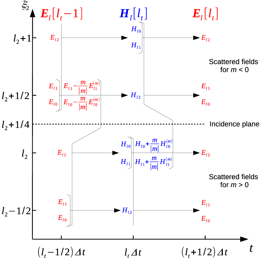
Figure 1 gives us an arrangement of discrete functions from the continuous functions $\boldsymbol{f}_{\xi}\boldsymbol{E}$ , $\boldsymbol{f}_{\xi}\boldsymbol{H}$ , ${\boldsymbol{\varepsilon}}_{\xi}$ and ${\boldsymbol{\mu}}_{\xi}$ , where the discrete functions are allocated at a cell address $\left[\boldsymbol{l}\right]$ . Discrete electromagnetic fields $\boldsymbol{f}_{\xi}\boldsymbol{E}\left(\boldsymbol{\xi}\right)\Rightarrow\boldsymbol{E}_{l}\left[\boldsymbol{l}\right]$ and $\boldsymbol{f}_{\xi}\boldsymbol{H}\left(\boldsymbol{\xi}\right)\Rightarrow\boldsymbol{H}_{l}\left[\boldsymbol{l}\right]$ are derived by eq. (4) and Fig. 1. The components of $\boldsymbol{E}_{l}\left[\boldsymbol{l}\right]$ and $\boldsymbol{H}_{l}\left[\boldsymbol{l}\right]$ are defined as

\left\{\begin{aligned} {E}_{lj}\left[\boldsymbol{l}\right]&\triangleq u_{j}^{{}^{\prime}}h_{j}E_{j}\left(l_{0}+\frac{1-\delta_{j0}}{2},\,l_{1}+\frac{1-\delta_{j1}}{2},\,l_{2}+\frac{1-\delta_{j2}}{2}\right)\,,\\ {H}_{lj}\left[\boldsymbol{l}\right]&\triangleq u_{j}^{{}^{\prime}}h_{j}H_{j}\left(l_{0}+\frac{\delta_{j0}}{2},\,l_{1}+\frac{\delta_{j1}}{2},\,l_{2}+\frac{\delta_{j2}}{2}\right)\,.\end{aligned}\right.

(5)

Discrete medium, which consists of ${\boldsymbol{\varepsilon}}_{\xi}\left(\boldsymbol{\xi}\right)\Rightarrow{\boldsymbol{\varepsilon}}_{l}\left[\boldsymbol{l}\right]$ and ${\boldsymbol{\mu}}_{\xi}\left(\boldsymbol{\xi}\right)\Rightarrow{\boldsymbol{\mu}}_{l}\left[\boldsymbol{l}\right]$ , is also derived by eq. (4) and Fig. 1. The components of ${\boldsymbol{\varepsilon}}_{l}\left[\boldsymbol{l}\right]$ and ${\boldsymbol{\mu}}_{l}\left[\boldsymbol{l}\right]$ are defined with PML factor $\tilde{\sigma}_{j}\left(\xi_{j}\right)$ from eq. (11) and correction factor $\eta_{j}$ from eqs. (3) and (4):

\left\{\begin{aligned} \varepsilon_{ljj}\left[\boldsymbol{l}\right]\triangleq\frac{u_{j+1}^{{}^{\prime}}u_{j+2}^{{}^{\prime}}h_{j+1}h_{j+2}}{u_{j}^{{}^{\prime}}h_{j}}&\frac{\left[1+i\tilde{\sigma}_{j+1}\left(l_{j+1}+1/2\right)\right]\left[1+i\tilde{\sigma}_{j+2}\left(l_{j+2}+1/2\right)\right]}{1+i\tilde{\sigma}_{j}\left(l_{j}\right)}\\ &\quad\times{}\frac{\varepsilon\left(l_{0}+\left({1-\delta_{j0}}\right)/{2},\,l_{1}+\left({1-\delta_{j1}}\right)/{2},\,l_{2}+\left({1-\delta_{j2}}\right)/{2}\right)}{1+\eta_{j}\left(l_{0}+\left({1-\delta_{j0}}\right)/{2},\,l_{1}+\left({1-\delta_{j1}}\right)/{2},\,l_{2}+\left({1-\delta_{j2}}\right)/{2}\right)}\,,\\ \mu_{ljj}\left[\boldsymbol{l}\right]\triangleq\frac{u_{j+1}^{{}^{\prime}}u_{j+2}^{{}^{\prime}}h_{j+1}h_{j+2}}{u_{j}^{{}^{\prime}}h_{j}}&\frac{\left[1+i\tilde{\sigma}_{j+1}\left(l_{j+1}\right)\right]\left[1+i\tilde{\sigma}_{j+2}\left(l_{j+2}\right)\right]}{1+i\tilde{\sigma}_{j}\left(l_{j}+1/2\right)}\\ &\quad\times{}\frac{\mu\left(l_{0}+{\delta_{j0}}/{2},\,l_{1}+{\delta_{j1}}/{2},\,l_{2}+{\delta_{j2}}/{2}\right)}{1+\eta_{j}\left(l_{0}+{\delta_{j0}}/{2},\,l_{1}+{\delta_{j1}}/{2},\,l_{2}+{\delta_{j2}}/{2}\right)}\,.\end{aligned}\right.

(6)

Numerical calculation considers finite numbers of Yee cells as $0\leq l_{j}<L_{j}$ . Function $\mathcal{G}\left[\boldsymbol{l}\right]$ , which is $H_{lj}$ for example, satisfies the following boundary conditions for $l_{0}$ and $l_{1}$ .

\left\{\begin{gathered}\mathcal{G}\left[L_{0},\,l_{1},\,l_{2}\right]=B_{0}\mathcal{G}\left[0,\,l_{1},\,l_{2}\right],\quad\mathcal{G}\left[-1,\,l_{1},\,l_{2}\right]=B_{0}^{*}\mathcal{G}\left[L_{0}-1,\,l_{1},\,l_{2}\right],\\ \mathcal{G}\left[l_{0},\,L_{1},\,\,l_{2}\right]=B_{1}\mathcal{G}\left[l_{0},\,0,\,l_{2}\right],\quad\mathcal{G}\left[l_{0},\,-1,\,\,l_{2}\right]=B_{1}^{*}\mathcal{G}\left[l_{0},\,L_{1}-1,\,l_{2}\right],\end{gathered}\right.

(7)

where $\left|B_{j}\right|=1\,\,\mathrm{or}\,\,0$ , and $\mathcal{G}=H_{lj}$ , $E_{lj}$ for example. The two parameters $B_{0}$ and $B_{1}$ are generally complex number, and we could choose a periodic condition $B_{j}=1$ or an anti-periodic condition $B_{j}=-1$ . We can also set $B_{0}=0$ when $\kappa_{b}\neq 0$ , since the system does not become periodic along the $u_{0}$ -axis.

Let us introduce forward and backward difference operators as

\left\{\begin{aligned} \bigtriangleup_{j}\mathcal{G}\left[l_{0},\,l_{1},\,l_{2}\right]&\triangleq\mathcal{G}\left[l_{0}+\delta_{j0},\,l_{1}+\delta_{j1},\,l_{2}+\delta_{j2}\right]-\mathcal{G}\left[l_{0},\,l_{1},\,l_{2}\right],\\ \bigtriangledown_{j}\mathcal{G}\left[l_{0},\,l_{1},\,l_{2}\right]&\triangleq\mathcal{G}\left[l_{0},\,l_{1},\,l_{2}\right]-\mathcal{G}\left[l_{0}-\delta_{j0},\,l_{1}-\delta_{j1},\,l_{2}-\delta_{j2}\right].\end{aligned}\right.

(8)

From eqs. (7) and (8), the difference operators at boundaries are given by

\left\{\begin{aligned} \bigtriangleup_{0}\mathcal{G}\left[L_{0}-1,\,l_{1},\,l_{2}\right]&=B_{0}\mathcal{G}\left[0,\,l_{1},\,l_{2}\right]-\mathcal{G}\left[L_{0}-1,\,l_{1},\,l_{2}\right],\;\bigtriangledown_{0}\mathcal{G}\left[0,\,l_{1},\,l_{2}\right]=\mathcal{G}\left[0,\,l_{1},\,l_{2}\right]-B_{0}^{*}\mathcal{G}\left[L_{0}-1,\,l_{1},\,l_{2}\right],\\ \bigtriangleup_{1}\mathcal{G}\left[l_{0},\,L_{1}-1,\,l_{2}\right]&=B_{1}\mathcal{G}\left[l_{0},\,0,\,l_{2}\right]-\mathcal{G}\left[l_{0},\,L_{1}-1,\,l_{2}\right],\;\bigtriangledown_{1}\mathcal{G}\left[l_{0},\,0,\,l_{2}\right]=\mathcal{G}\left[l_{0},\,0,\,l_{2}\right]-B_{1}^{*}\mathcal{G}\left[l_{0},\,L_{1}-1,\,l_{2}\right].\end{aligned}\right.

Therefore, discrete difference operators satisfy $\bigtriangledown_{j}=-\bigtriangleup_{j}^{\dagger}$ , but $\bigtriangleup_{j}\neq-\bigtriangleup_{j}^{\dagger}$ . This relation is different from the case of continuous difference operators $\partial_{j}=-\partial_{j}^{\dagger}$ under the boundary condition of eq. (7).

From eqs. (5), (6) and Fig. 1, the deformed Maxwell equation (3) could be discretized into

\left(\begin{array}[]{cc}0&i\boldsymbol{R}\\ -i\boldsymbol{R}^{\dagger}&0\end{array}\right)\left(\begin{array}[]{c}\boldsymbol{E}_{l}\\ \boldsymbol{H}_{l}\end{array}\right)=\omega\left(\begin{array}[]{cc}{\boldsymbol{\varepsilon}}_{l}&0\\ 0&{\boldsymbol{\mu}}_{l}\end{array}\right)\left(\begin{array}[]{c}\boldsymbol{E}_{l}\\ \boldsymbol{H}_{l}\end{array}\right),

(9)

where the discrete rotation operators $\boldsymbol{R}$ and $\boldsymbol{R}^{\dagger}$ are defined by using eqs. (8):

\boldsymbol{R}\triangleq\left(\begin{array}[]{ccc}0&-\bigtriangleup_{2}&\bigtriangleup_{1}\\ \bigtriangleup_{2}&0&-\bigtriangleup_{0}\\ -\bigtriangleup_{1}&\bigtriangleup_{0}&0\end{array}\right)\quad\mathrm{and}\quad\boldsymbol{R}^{\dagger}\triangleq\left(\begin{array}[]{ccc}0&\bigtriangleup_{2}^{\dagger}&-\bigtriangleup_{1}^{\dagger}\\ -\bigtriangleup_{2}^{\dagger}&0&\bigtriangleup_{0}^{\dagger}\\ \bigtriangleup_{1}^{\dagger}&-\bigtriangleup_{0}^{\dagger}&0\end{array}\right)=\left(\begin{array}[]{ccc}0&-\bigtriangledown_{2}&\bigtriangledown_{1}\\ \bigtriangledown_{2}&0&-\bigtriangledown_{0}\\ -\bigtriangledown_{1}&\bigtriangledown_{0}&0\end{array}\right).

(10)

The $\boldsymbol{R}$ and $\boldsymbol{R}^{\dagger}$ are used in eq. (1).

[Go to table of contents.] [Go to home.]

Chapter 6 Propagation equation for Yee’s lattice

This chapter shows discrete formulae derived from the discrete Maxwell-equation (9).

1 Discrete propagation-equation

Discrete formulation can be represented as similar to propagation equation (1) with eq. (13). In order to simplify mathematical notations , we only show a discrete parameter $l_{2}$ instead of $\boldsymbol{l}$ in the following equations.

\boldsymbol{M}_{\pm}\boldsymbol{\Psi}_{\pm}=-i\left(\begin{array}[]{cc}\boldsymbol{0}&\bigtriangledown_{2}\\ \bigtriangleup_{2}&\boldsymbol{0}\end{array}\right)\boldsymbol{\Psi}_{\pm}\quad\mathrm{as}\quad\left\{\begin{aligned} \boldsymbol{M}_{+}&\triangleq\left(\begin{array}[]{cc}\boldsymbol{m}_{aa}\left(\boldsymbol{V}\left[l_{2}\right]\right)&\boldsymbol{0}\\ \boldsymbol{0}&\boldsymbol{m}_{bb}\left(\boldsymbol{V}\left[l_{2}\right]\right)\end{array}\right),\\ \boldsymbol{M}_{-}&\triangleq\left(\begin{array}[]{cc}\boldsymbol{m}_{bb}\left(\boldsymbol{V}\left[l_{2}\right]\right)&\boldsymbol{0}\\ \boldsymbol{0}&\boldsymbol{m}_{aa}\left(\boldsymbol{V}\left[l_{2}+1\right]\right)\end{array}\right).\end{aligned}\right.

(1)

The subscript $+$ ( $-$ ) in eq. (1) means a configuration as advanced (retarded) electric fields to magnetic fields. From eq. (4), the discrete $\boldsymbol{m}_{aa}$ , $\boldsymbol{m}_{bb}$ and $\boldsymbol{\Psi}_{\pm}$ are defined by

\left\{\begin{gathered}\boldsymbol{m}_{aa}\left(\boldsymbol{V}\right)=\left(\begin{array}[]{cc}{V}_{0}+\bigtriangledown_{1}{V}_{2}\bigtriangleup_{1}&-\bigtriangledown_{1}{V}_{2}\bigtriangleup_{0}\\ -\bigtriangledown_{0}{V}_{2}\bigtriangleup_{1}&{V}_{1}+\bigtriangledown_{0}{V}_{2}\bigtriangleup_{0}\end{array}\right),\quad\boldsymbol{m}_{bb}\left(\boldsymbol{V}\right)=\left(\begin{array}[]{cc}{V}_{3}+\bigtriangleup_{0}{V}_{5}\bigtriangledown_{0}&\bigtriangleup_{0}{V}_{5}\bigtriangledown_{1}\\ \bigtriangleup_{1}{V}_{5}\bigtriangledown_{0}&{V}_{4}+\bigtriangleup_{1}{V}_{5}\bigtriangledown_{1}\end{array}\right),\\ {V}_{0}=\omega\mu_{l00},\quad{V}_{1}=\omega\mu_{l11},\quad{V}_{2}=\frac{1}{\omega\varepsilon_{l22}},\quad{V}_{3}=\omega\varepsilon_{l11},\quad{V}_{4}=\omega\varepsilon_{l00},\quad{V}_{5}=\frac{1}{\omega\mu_{l22}},\\ \boldsymbol{\Psi}_{+}\left[l_{2}\right]\triangleq\left(\begin{array}[]{c}\boldsymbol{H}_{2D}\left[l_{2}\right]\\ \boldsymbol{E}_{2D}\left[l_{2}\right]\end{array}\right),\;\boldsymbol{\Psi}_{-}\left[l_{2}\right]\triangleq\left(\begin{array}[]{c}\boldsymbol{E}_{2D}\left[l_{2}\right]\\ \boldsymbol{H}_{2D}\left[l_{2}+1\right]\end{array}\right),\\ \boldsymbol{H}_{2D}\left[l_{2}\right]=\left(\begin{array}[]{c}H_{l0}\left[l_{2}\right]\\ H_{l1}\left[l_{2}\right]\end{array}\right),\;\boldsymbol{E}_{2D}\left[l_{2}\right]=\left(\begin{array}[]{c}-E_{l1}\left[l_{2}\right]\\ E_{l0}\left[l_{2}\right]\end{array}\right).\end{gathered}\right.

(2)

The operators $\bigtriangleup_{j}$ and $\bigtriangledown_{j}$ for $j=0,1$ in $\boldsymbol{m}_{aa}$ and $\boldsymbol{m}_{bb}$ of eq. (2) can be regarded as $L_{0}L_{1}\times L_{0}L_{1}$ matrices. The ${V}_{0},\cdots,{V}_{5}$ also become $L_{0}L_{1}\times L_{0}L_{1}$ diagonal matrices, and then $\boldsymbol{V}$ can be set as a $6L_{0}L_{1}\times 6L_{0}L_{1}$ diagonal matrix. The $\mu_{ljj}$ and $\varepsilon_{ljj}$ in eq. (2) were defined by eq. (6). The factor $\sqrt{du_{0}du_{1}}/2$ of eq. (11) is removed from the discrete $\boldsymbol{\Psi}$ in eq. (2), since it does not affect the following discussion. The $H_{lj}$ and $E_{lj}$ for $j=0,1$ are $L_{0}L_{1}\times 1$ column vectors. Note that $\boldsymbol{M}_{\pm}=\boldsymbol{M}_{\pm}^{\dagger}$ when $\varepsilon$ and $\mu$ are real number.

We define two types of power flow for eq. (1) as similar to the first of eq. (2):

P_{\pm}\left[l_{2}\right]\triangleq\boldsymbol{\Psi}_{\pm}^{\dagger}\left[l_{2}\right]\left(\begin{array}[]{cc}0&1\\ 1&0\end{array}\right)\boldsymbol{\Psi}_{\pm}\left[l_{2}\right].

From the above definition and eq. (5), we show two relations for $P_{\pm}$ as follows.

\left\{\begin{aligned} P_{+}\left[l_{2}\right]-P_{-}\left[l_{2}-1\right]&=i\boldsymbol{H}_{2D}^{\dagger}\left[l_{2}\right]\left(\boldsymbol{m}_{aa}\left[l_{2}\right]-\boldsymbol{m}_{aa}^{\dagger}\left[l_{2}\right]\right)\boldsymbol{H}_{2D}\left[l_{2}\right],\\ P_{-}\left[l_{2}\right]-P_{+}\left[l_{2}\right]&=i\boldsymbol{E}_{2D}^{\dagger}\left[l_{2}\right]\left(\boldsymbol{m}_{bb}\left[l_{2}\right]-\boldsymbol{m}_{bb}^{\dagger}\left[l_{2}\right]\right)\boldsymbol{E}_{2D}\left[l_{2}\right].\end{aligned}\right.

(3)

Note that $P_{+}=P_{-}$ when $\boldsymbol{M}_{+}^{\dagger}=\boldsymbol{M}_{+}$ . Equation (3) gives us conservation rule of ${\Psi}_{\pm}$ as similar to the second of eq. (2):

\bigtriangleup_{2}P_{+}=i\boldsymbol{\Psi}_{-}^{\dagger}\left(\boldsymbol{M}_{-}-\boldsymbol{M}_{-}^{\dagger}\right)\boldsymbol{\Psi}_{-}^{\dagger}\quad\mathrm{and}\quad\bigtriangledown_{2}P_{-}=i\boldsymbol{\Psi}_{+}^{\dagger}\left(\boldsymbol{M}_{+}-\boldsymbol{M}_{+}^{\dagger}\right)\boldsymbol{\Psi}_{+}^{\dagger}\,.

In the following discussion, we only use the configuration with subscript $+$ for eqs. (1) and (2), since it can be directly associated with $H_{lj}$ and $E_{lj}$ of the Yee cell in Fig. 1. The subscript $+$ will be abbreviated as $\boldsymbol{\Psi}$ .

From eq. (6), we can define transfer matrix $\boldsymbol{T}_{RL}\left[l_{2}\right]$ as follows.

\boldsymbol{\Psi}\left[l_{2}+1\right]=\boldsymbol{T}_{RL}\left[l_{2}\right]\boldsymbol{\Psi}\left[l_{2}\right]\quad\mathrm{as}\quad\boldsymbol{T}_{RL}\left[l_{2}\right]\triangleq\left(\begin{array}[]{cc}1&i\boldsymbol{m}_{bb}\left[l_{2}\right]\\ i\boldsymbol{m}_{aa}\left[l_{2}+1\right]&1-\boldsymbol{m}_{aa}\left[l_{2}+1\right]\boldsymbol{m}_{bb}\left[l_{2}\right]\end{array}\right).

(4)

2 Discrete mode-equation

This section considers a scattering region and two outer regions. The scattering region is in $0\leq l_{2}<L_{2}$ , and the outer regions are in $l_{2}<0$ and $l_{2}\geq L_{2}$ , i.e. $\left|L_{2}-1-2l_{2}\right|>L_{2}-1$ . The outer region set that the $\boldsymbol{m}_{aa}$ and $\boldsymbol{m}_{bb}$ are not depend on $l_{2}$ , and $\boldsymbol{m}_{aa}=\boldsymbol{m}_{aa}^{\dagger}$ and $\boldsymbol{m}_{bb}=\boldsymbol{m}_{bb}^{\dagger}$ . The definitions in eq. (2) derive that

\boldsymbol{m}_{aa}^{\dagger}=\boldsymbol{m}_{aa}^{*}=\boldsymbol{m}_{aa}\quad\mathrm{and}\quad\boldsymbol{m}_{bb}^{\dagger}=\boldsymbol{m}_{bb}^{*}=\boldsymbol{m}_{bb}\,.

(5)

By using definition of eq. (1), $\boldsymbol{m}^{\left(0\right)}_{aa}$ and $\boldsymbol{m}^{\left(0\right)}_{bb}$ satisfy eq. (5) even in the scattering region. Discrete mode-function $\boldsymbol{\Phi}_{m}$ as similar to eq. (1) could be given by solving an eigenvalue equation.

\left(\begin{array}[]{cc}\boldsymbol{m}^{\left(0\right)}_{aa}\left[l_{2}\right]&\boldsymbol{0}\\ \boldsymbol{0}&\boldsymbol{m}^{\left(0\right)}_{bb}\left[l_{2}\right]\end{array}\right)\boldsymbol{\Phi}_{m}\left[l_{2}\right]=2\sin\left({\theta_{m}\left[l_{2}\right]}/{2}\right)\left(\begin{array}[]{cc}0&1\\ 1&0\end{array}\right)\boldsymbol{\Phi}_{m}\left[l_{2}\right]\quad\mathrm{as}\quad\boldsymbol{\Phi}_{m}\left[l_{2}\right]\triangleq\left(\begin{array}[]{c}\boldsymbol{h}_{m}\left[l_{2}\right]\\ \boldsymbol{e}_{m}\left[l_{2}\right]\end{array}\right).

(6)

Note that $\sin a\triangleq-i\left(e^{ia}-e^{-ia}\right)/2$ , and then $\left(\sin a\right)^{*}=i\left(e^{-ia^{*}}-e^{ia^{*}}\right)/2=\sin a^{*}$ . The cosine and the tangent are also defined in the same manner. Orthogonality and normalization for the discrete $\boldsymbol{\Phi}_{m}$ are given by

\boldsymbol{\Phi}_{n}^{\dagger}\left(\begin{array}[]{cc}0&1\\ 1&0\end{array}\right)\boldsymbol{\Phi}_{m}=\boldsymbol{h}_{n}^{\dagger}\boldsymbol{e}_{m}+\boldsymbol{e}_{n}^{\dagger}\boldsymbol{h}_{m}=\begin{cases}\frac{m}{\left|m\right|}\frac{\delta_{n\,m}}{\cos\left(\theta_{m}/2\right)}&\mathrm{for}\quad 0<\left|m\right|\leq n_{\max}\,,\\ \frac{\delta_{-n\,m}}{\cos\left(\theta_{m}/2\right)}&\mathrm{for}\quad\left|m\right|>n_{\max}\,.\end{cases}

where the above numbering rule is the same as the rule of Section 1. Note that the denominator $\cos\left(\theta_{m}/2\right)$ in the normalization is caused by the discretization, and it is different from the case in Section 2. Small $\theta_{m}$ is related to the propagation constant $\beta_{m}$ in eq. (1) by referring to Section 2 and eq. (6):

\beta_{m}=\lim_{h_{2}{u_{2}^{{}^{\prime}}}\rightarrow 0}\frac{2\sin\left({\theta_{m}}/{2}\right)}{h_{2}{u_{2}^{{}^{\prime}}}}\simeq\frac{{\theta_{m}}}{h_{2}{u_{2}^{{}^{\prime}}}}\,.

Equation (6) gives us a reduced eigenvalue-equation of $\boldsymbol{h}_{m}$ ( or $\boldsymbol{e}_{m}$ ) and a relation between $\boldsymbol{e}_{m}$ and $\boldsymbol{h}_{m}$ :

\left\{\begin{aligned} \boldsymbol{m}^{\left(0\right)}_{bb}\boldsymbol{m}^{\left(0\right)}_{aa}\boldsymbol{h}_{m}&=4\sin^{2}\left({\theta_{m}}/{2}\right)\boldsymbol{h}_{m}\,,\\ \boldsymbol{e}_{m}&=\frac{\boldsymbol{m}^{\left(0\right)}_{aa}\boldsymbol{h}_{m}}{2\sin\left({\theta_{m}}/{2}\right)}\,.\end{aligned}\right.\quad\left(\,\mathrm{or}\quad\left\{\begin{aligned} \boldsymbol{m}^{\left(0\right)}_{aa}\boldsymbol{m}^{\left(0\right)}_{bb}\boldsymbol{e}_{m}&=4\sin^{2}\left({\theta_{m}}/{2}\right)\boldsymbol{e}_{m}\,,\\ \boldsymbol{h}_{m}&=\frac{\boldsymbol{m}^{\left(0\right)}_{bb}\boldsymbol{e}_{m}}{2\sin\left({\theta_{m}}/{2}\right)}\,.\end{aligned}\right.\quad\right)

(7)

The $\boldsymbol{h}_{m}$ and $\boldsymbol{e}_{m}$ become real vector if $\sin\left({\theta_{m}}/{2}\right)$ is real, since $\boldsymbol{m}_{aa}$ and $\boldsymbol{m}_{bb}$ are real matrix from eq. (5). Furthermore, $\boldsymbol{e}_{n}^{\mathrm{T}}\boldsymbol{h}_{m}=0$ if $\sin^{2}\left({\theta_{m}}/{2}\right)\neq\sin^{2}\left({\theta_{n}}/{2}\right)$ for real $\sin\left({\theta_{m}}/{2}\right)$ and $\sin\left({\theta_{n}}/{2}\right)$ . However, we have to be careful in handling eigenvectors (i.e. modes) for other case as discussed in Section 2. From the definition in eq. (6) and the relation of $\boldsymbol{h}_{m}$ and $\boldsymbol{e}_{m}$ in eq. (7), the orthogonality and normalization of the $\boldsymbol{\Phi}_{m}$ are reduced to

\begin{cases}\boldsymbol{h}_{n}^{\mathrm{T}}\boldsymbol{e}_{m}=\boldsymbol{e}_{n}^{\mathrm{T}}\boldsymbol{h}_{m}=\frac{m\delta_{n\,m}}{2\left|m\right|\cos\left(\theta_{m}/2\right)}&\mathrm{for}\quad 0<\left|m\right|\leq n_{\max}\,,\\ \boldsymbol{h}_{n}^{\dagger}\boldsymbol{e}_{m}=\boldsymbol{e}_{n}^{\dagger}\boldsymbol{h}_{m}=\frac{\delta_{-n\,m}}{2\cos\left(\theta_{m}/2\right)}&\mathrm{for}\quad\left|m\right|>n_{\max}\,.\end{cases}

(8)

Furthermore, we can add special relations

\boldsymbol{h}_{-m}=\boldsymbol{h}_{m}\quad\mathrm{and}\quad\boldsymbol{e}_{-m}=-\boldsymbol{e}_{m}\quad\mathrm{for}\quad 0<\left|m\right|\leq n_{\max}

(9)

to eq. (8) without loss of generality. Discrete electromagnetic field $\boldsymbol{\Psi}_{+}\left[l_{2}\right]$ in eq. (2) for $\left|2l_{2}+1-L_{2}\right|>L_{2}$ can be expanded into series of modified mode function $\boldsymbol{\Xi}_{m}$ :

\boldsymbol{\Psi}_{+}\left[l_{2}\right]=\sum_{m\neq 0}c_{m}\exp\left(i\theta_{m}l_{2}\right)\boldsymbol{\Xi}_{m}\quad\mathrm{as}\quad\boldsymbol{\Xi}_{m}\triangleq\left(\begin{array}[]{cc}\exp\left(-i\theta_{m}/2\right)&0\\ 0&1\end{array}\right)\left(\begin{array}[]{c}\boldsymbol{h}_{m}\\ \boldsymbol{e}_{m}\end{array}\right).

(10)

By checking eq. (7), we can confirm that the above expansion has consistency with the discrete propagation equation (1). The $\boldsymbol{\Xi}_{m}$ maintains the orthogonality as

\boldsymbol{\Xi}_{n}^{\dagger}\left(\begin{array}[]{cc}0&1\\ 1&0\end{array}\right)\boldsymbol{\Xi}_{m}=\boldsymbol{h}_{n}^{\dagger}\exp\left(i\frac{\theta_{n}^{*}}{2}\right)\boldsymbol{e}_{m}+\boldsymbol{e}_{n}^{\dagger}\exp\left(-i\frac{\theta_{m}}{2}\right)\boldsymbol{h}_{m}=\begin{cases}\frac{m}{\left|m\right|}\delta_{n\,m}&\mathrm{for}\quad 0<\left|m\right|\leq n_{\max}\,,\\ \delta_{-n\,m}&\mathrm{for}\quad\left|m\right|>n_{\max}\,.\end{cases}

(11)

The power flow $P_{+}$ is represented by $c_{m}$ from eqs. (10) and (11):

P_{+}\left[l_{2}\right]=\boldsymbol{\Psi}_{+}^{\dagger}\left[l_{2}\right]\left(\begin{array}[]{cc}0&1\\ 1&0\end{array}\right)\boldsymbol{\Psi}_{+}\left[l_{2}\right]=\sum_{0<\left|m\right|\leq n_{\max}}\frac{m}{\left|m\right|}\left|c_{m}\right|^{2}+\sum_{\left|m\right|>n_{\max}}c_{-m}^{*}c_{m}\,.

3 Discrete scattering-matrix

Scattering matrix of eq. (14) can be discretized by the discrete propagation-equation (1) and the modified mode function (10).

S_{mn}\triangleq\exp\left(-i\Theta_{n}\left[b_{m}\right]\right)\boldsymbol{\Xi}_{m}^{\dagger}\left[b_{m}\right]\frac{m}{\left|m\right|}\left(\begin{array}[]{cc}0&1\\ 1&0\end{array}\right)\boldsymbol{\Psi}_{n}\left[b_{m}\right]

(12)

for $0<\left|m\right|\leq n_{\max}$ and $0<\left|n\right|\leq n_{\max}$ . The $b_{m}$ in the right-hand side of eq. (12) is redefined as

b_{m}=\frac{\left|m\right|+m}{2\left|m\right|}\left(L_{2}-1\right)=\begin{cases}L_{2}-1&\mathrm{for}\quad m>0\,,\\ 0&\mathrm{for}\quad m<0\,,\end{cases}

and $\Theta_{n}\left[b_{m}\right]$ is given by eq. (8):

\begin{split}\frac{m}{\left|m\right|}\Theta_{n}\left[b_{m}\right]&\triangleq\sum_{\frac{b_{m}}{2}\leq l_{2}<\frac{L_{2}-1+b_{m}}{2}}\frac{\theta_{n}\left[l_{2}\right]}{2}+\sum_{\frac{b_{m}}{2}<l_{2}\leq\frac{L_{2}-1+b_{m}}{2}}\frac{\theta_{n}\left[l_{2}\right]}{2}\\ &=\begin{cases}\frac{\theta_{n}\left[\frac{L_{2}-1}{2}\right]}{2}+\sum_{\frac{L_{2}-1}{2}<l_{2}<L_{2}-1}\theta_{n}\left[l_{2}\right]+\frac{\theta_{n}\left[L_{2}-1\right]}{2}&\mathrm{for}\quad m>0\quad\mathrm{and}\quad L_{2}=\mathrm{odd}\,,\\ \qquad\qquad\quad\sum_{\frac{L_{2}-1}{2}<l_{2}<L_{2}-1}\theta_{n}\left[l_{2}\right]+\frac{\theta_{n}\left[L_{2}-1\right]}{2}&\mathrm{for}\quad m>0\quad\mathrm{and}\quad L_{2}=\mathrm{even}\,,\\ \frac{\theta_{n}\left[0\right]}{2}+\sum_{0<l_{2}<\frac{L_{2}-1}{2}}\theta_{n}\left[l_{2}\right]+\frac{\theta_{n}\left[\frac{L_{2}-1}{2}\right]}{2}&\mathrm{for}\quad m<0\quad\mathrm{and}\quad L_{2}=\mathrm{odd}\,,\\ \frac{\theta_{n}\left[0\right]}{2}+\sum_{0<l_{2}<\frac{L_{2}-1}{2}}\theta_{n}\left[l_{2}\right]&\mathrm{for}\quad m<0\quad\mathrm{and}\quad L_{2}=\mathrm{even}\,.\end{cases}\end{split}

(13)

The $\boldsymbol{\Psi}_{n}$ in eq. (12) is redefined as a particular solution of $\boldsymbol{\Psi}_{+}$ in eq. (2), which satisfies boundary conditions at outer regions:

\boldsymbol{\Psi}_{n}\left[b_{m}\right]=\exp\left(i\Theta_{n}\left[b_{m}\right]\right)\left(\frac{\left|mn\right|-mn}{2\left|mn\right|}\boldsymbol{\Xi}_{n}\left[b_{m}\right]+\sum_{0<\frac{m^{{}^{\prime}}m}{\left|m\right|}\leq n_{\max}}S_{m^{{}^{\prime}}n}\boldsymbol{\Xi}_{m^{{}^{\prime}}}\left[b_{m}\right]\right).

(14)

The following discussion is based on the framework of Section 16.E. Equation (9) at $l_{2}=b_{m}$ shows that

\begin{split}\boldsymbol{\Psi}_{n}\left[b_{m}\right]&=\exp\left(i\Theta_{n}\left[b_{m}\right]\right)\left(\boldsymbol{\Xi}_{n}\left[b_{m}\right]+\sum_{1\leq j<L_{2}-1}\boldsymbol{G}\left[b_{m},j\right]\right),\\ \boldsymbol{G}\left[b_{m},j\right]&=\sum_{0<\frac{m^{{}^{\prime}}m}{\left|m\right|}\leq n_{\max}}g_{m^{{}^{\prime}}n}\left[j\right]\exp\left\{i\left(\Theta_{m^{{}^{\prime}}}\left[b_{m}\right]-\Theta_{n}\left[b_{m}\right]\right)-i\left(\Theta_{m^{{}^{\prime}}}\left[j\right]-\Theta_{n}\left[j\right]\right)\right\}\boldsymbol{\Xi}_{m^{{}^{\prime}}}\left[b_{m}\right]\,.\end{split}

By comparing the above equations and eq. (14), the $S_{mn}$ is related to the $g_{mn}$ :

S_{mn}-\delta_{mn}=\sum_{1\leq j<L_{2}-1}g_{mn}\left[j\right]\exp\left\{i\left(\Theta_{m}\left[b_{m}\right]-\Theta_{n}\left[b_{m}\right]\right)-i\left(\Theta_{m}\left[j\right]-\Theta_{n}\left[j\right]\right)\right\}\,.

(15)

When ${\boldsymbol{M}}_{+}^{\left(0\right)}$ in eq. (10) is independent of $l_{2}$ , the $S_{mn}$ of eq.(15) is simplified to

S_{mn}-\delta_{mn}=\sum_{0\leq j<L_{2}}g_{mn}\left[j\right]\exp\left\{i\left(\theta_{m}\left[b_{m}-j\right]-\theta_{n}\left[b_{m}-j\right]\right)\right\}=\exp\left(i\frac{m}{\left|m\right|}\left(\theta_{m}-\theta_{n}\right)\frac{L_{2}-1}{2}\right)\widehat{g_{mn}}_{\mathrm{DFT}}\left(\theta_{m}-\theta_{n}\right),

where $g_{mn}\left[0\right]=g_{mn}\left[L_{2}-1\right]=0$ , and “ $\,\widehat{\quad}_{\mathrm{DFT}}$ ” is defined by eq. (22). From detail of the $\widehat{g_{mn}}_{\mathrm{DFT}}$ in eq. (20), the above equation is represented as

\begin{split}\left|S_{mn}-\delta_{mn}\right|^{2}&=\left|\widehat{g_{mn}}_{\mathrm{DFT}}\left(\theta_{m}-\theta_{n}\right)\right|^{2}=\left|\boldsymbol{\Xi}_{m}^{\dagger}\left(\begin{array}[]{cc}e^{i\theta_{m}}\widehat{\boldsymbol{m}_{aa}^{\left(1\right)}}_{\mathrm{DFT}}\left(\theta_{m}-\theta_{n}\right)&\boldsymbol{0}\\ \boldsymbol{0}&e^{-i\theta_{m}}\widehat{\boldsymbol{m}_{bb}^{\left(1\right)}}_{\mathrm{DFT}}\left(\theta_{m}-\theta_{n}\right)\end{array}\right)\boldsymbol{\Xi}_{n}\right|^{2}\\ &=\left|e^{i\theta_{m}}e^{i\left(\theta_{m}-\theta_{n}\right)/2}\boldsymbol{h}_{m}^{\mathrm{T}}\left[\widehat{\boldsymbol{m}_{aa}^{\left(1\right)}}_{\mathrm{DFT}}\left(\theta_{m}-\theta_{n}\right)\right]\boldsymbol{h}_{n}+e^{-i\theta_{m}}\boldsymbol{e}_{m}^{\mathrm{T}}\left[\widehat{\boldsymbol{m}_{bb}^{\left(1\right)}}_{\mathrm{DFT}}\left(\theta_{m}-\theta_{n}\right)\right]\boldsymbol{e}_{n}\right|^{2}.\end{split}

(16)

4 Discrete edge-roughness scattering of Section 13.B

This section shows $\widehat{\boldsymbol{m}_{aa}^{\left(1\right)}}_{\mathrm{DFT}}$ and $\widehat{\boldsymbol{m}_{bb}^{\left(1\right)}}_{\mathrm{DFT}}$ in eq. (16) by separating unperturbed part $\boldsymbol{V}^{\left(0\right)}$ and perturbed part $\boldsymbol{V}^{\left(1\right)}$ from the discrete $\boldsymbol{V}$ in eq. (2). Elements of $\boldsymbol{V}^{\left(0\right)}$ are given by

{V}_{0}^{\left(0\right)}=\omega\mu_{l00},\quad{V}_{1}^{\left(0\right)}=\omega\mu_{l11},\quad{V}_{2}^{\left(0\right)}=\frac{1}{\omega\varepsilon_{l22}},\quad{V}_{3}^{\left(0\right)}=\omega\varepsilon_{l11},\quad{V}_{4}^{\left(0\right)}=\omega\varepsilon_{l00},\quad{V}_{5}^{\left(0\right)}=\frac{1}{\omega\mu_{l22}},

where $\boldsymbol{V}^{\left(0\right)}$ is not depend on $u_{2}$ . The DFT of $\boldsymbol{V}^{\left(1\right)}$ can be approximated to the FT with care of phase shift caused by half shift in eq. (6).

\widehat{{V}^{\left(1\right)}_{j+3J}}_{\mathrm{DFT}}\left(\phi\right)\simeq\frac{e^{i\phi J/2}}{u^{{}^{\prime}}_{2}}\widehat{{V}^{\left(1\right)}_{j+3J}}\left(\frac{\phi}{u^{{}^{\prime}}_{2}}\right)\quad\mathrm{for}\quad\left\{\begin{aligned} j&=0,1,2,\\ J&=0,1,\end{aligned}\right.

when $u^{{}^{\prime}}_{2}/L_{\mathrm{s}}$ is small, i.e. $L_{2}\gg 1$ from eq. (23). Then,

\widehat{\boldsymbol{m}_{aa}^{\left(1\right)}}_{\mathrm{DFT}}\left(\phi\right)=\frac{\sqrt{L_{\mathrm{s}}}}{u^{{}^{\prime}}_{2}}\boldsymbol{m}_{aa}\left(\frac{1}{\sqrt{L_{\mathrm{s}}}}\widehat{\boldsymbol{V}^{\left(1\right)}}\left(\frac{\phi}{u^{{}^{\prime}}_{2}}\right)\right),\quad\widehat{\boldsymbol{m}_{bb}^{\left(1\right)}}_{\mathrm{DFT}}\left(\phi\right)=\frac{e^{i\phi/2}\sqrt{L_{\mathrm{s}}}}{u^{{}^{\prime}}_{2}}\boldsymbol{m}_{bb}\left(\frac{1}{\sqrt{L_{\mathrm{s}}}}\widehat{\boldsymbol{V}^{\left(1\right)}}\left(\frac{\phi}{u^{{}^{\prime}}_{2}}\right)\right).

Note that $\boldsymbol{m}_{aa}$ ( $\boldsymbol{m}_{bb}$ ) is a function of only $V_{0}$ , $V_{1}$ and $V_{2}$ ( $V_{3}$ , $V_{4}$ and $V_{5}$ ). Equation (16) is represented as

\left\{\begin{aligned} \left|S_{mn}-\delta_{mn}\right|^{2}&=\frac{L_{\mathrm{s}}}{{u^{{}^{\prime}}_{2}}^{2}}\left|e^{i\theta_{m}}\boldsymbol{h}_{m}^{\mathrm{T}}\left[\boldsymbol{m}_{aa}\left(\frac{1}{\sqrt{L_{\mathrm{s}}}}\widehat{\boldsymbol{V}^{\left(1\right)}}\left(k_{mn}\right)\right)\right]\boldsymbol{h}_{n}+e^{-i\theta_{m}}\boldsymbol{e}_{m}^{\mathrm{T}}\left[\boldsymbol{m}_{bb}\left(\frac{1}{\sqrt{L_{\mathrm{s}}}}\widehat{\boldsymbol{V}^{\left(1\right)}}\left(k_{mn}\right)\right)\right]\boldsymbol{e}_{n}\right|^{2},\\ k_{mn}&=\frac{\theta_{m}-\theta_{n}}{u^{{}^{\prime}}_{2}}.\end{aligned}\right.

(17)

We can estimate roughness scattering by using eq. (17) with the following eq. (19) or (21). Therefore, we should crosscheck numerical results against another approach.

1 Discrete representation of Approach I for 1

This subsection considers that the $\boldsymbol{V}$ is a function of $A_{\mathrm{w}}$ and $A_{\mathrm{c}}$ as shown in Fig. 2. Here, we use eq. (6) for $h_{0}=h_{2}=1$ and constant $u^{{}^{\prime}}_{2}$ . By using the framework of eq. (4), elements of $\boldsymbol{V}^{\left(1\right)}\left(A_{\mathrm{w}},A_{\mathrm{c}}\right)$ are given as

\begin{split}{V}_{j+3J}^{\left(1\right)}\left(A_{\mathrm{w}},A_{\mathrm{c}}\right)&=\frac{{V}_{j+3J}\left(\frac{\varDelta A_{\mathrm{w}}}{2},0\right)-{V}_{j+3J}\left(-\frac{\varDelta A_{\mathrm{w}}}{2},0\right)}{\varDelta A_{\mathrm{w}}}A_{\mathrm{w}}\left(u_{2}\left(l_{2}+J/2\right)\right)\\ &\quad+\frac{{V}_{j+3J}\left(0,\frac{\varDelta A_{\mathrm{c}}}{2}\right)-{V}_{j+3J}\left(0,-\frac{\varDelta A_{\mathrm{c}}}{2}\right)}{\varDelta A_{\mathrm{c}}}A_{\mathrm{c}}\left(u_{2}\left(l_{2}+J/2\right)\right)\end{split}\quad\mathrm{for}\quad\left\{\begin{aligned} j&=0,1,2,\\ J&=0,1,\end{aligned}\right.

(18)

where $\varDelta A_{\mathrm{w}}$ and $\varDelta A_{\mathrm{c}}$ are parameters of finite difference, and we usually set $u^{{}^{\prime}}_{0}\lesssim\varDelta A_{\mathrm{w}}/2=\varDelta A_{\mathrm{c}}\lesssim 2u^{{}^{\prime}}_{0}$ . By using eq. (18), the $\widehat{\boldsymbol{V}^{\left(1\right)}}/\sqrt{L_{\mathrm{s}}}$ in eq. (17) can be given as

\frac{1}{\sqrt{L_{\mathrm{s}}}}\widehat{\boldsymbol{V}^{\left(1\right)}}\left(k_{mn}\right)=\frac{\boldsymbol{V}\left(\frac{\varDelta A_{\mathrm{w}}}{2},0\right)-\boldsymbol{V}\left(-\frac{\varDelta A_{\mathrm{w}}}{2},0\right)}{\varDelta A_{\mathrm{w}}}\widehat{a_{\mathrm{w}}}\left(k_{mn}\right)+\frac{\boldsymbol{V}\left(0,\frac{\varDelta A_{\mathrm{c}}}{2}\right)-\boldsymbol{V}\left(0,-\frac{\varDelta A_{\mathrm{c}}}{2}\right)}{\varDelta A_{\mathrm{c}}}\widehat{a_{\mathrm{c}}}\left(k_{mn}\right)\,.

(19)

2 Discrete representation of Approach II for 2

This subsection uses the parameter $s_{j+3J}\left(u_{0},u_{2}\right)$ of eq. (8) as

u_{0}\left(l_{0}+\frac{\left[\left(j+1\right)\%3\right]\%2+\left\{\left[\left(j+2\right)\%3\right]\%2\right\}\left(1-J\right)}{2}\right),\quad u_{2}\left(l_{2}+\frac{J}{2}\right)=\left[l_{2}+\frac{J}{2}-\frac{L_{2}}{2}\right]u^{{}^{\prime}}_{2}\quad\mathrm{for}\quad\left\{\begin{aligned} j&=0,1,2,\\ J&=0,1.\end{aligned}\right.

(20)

By using eq. (9) and the $u_{0}$ in eq. (20), elements of the $\widehat{\boldsymbol{V}^{\left(1\right)}}/\sqrt{L_{\mathrm{s}}}$ in eq. (17) can be given as

\frac{1}{\sqrt{L_{\mathrm{s}}}}\widehat{{V}^{\left(1\right)}_{j+3J}}\left(k_{mn}\right)={V}^{\left(0\right)}_{j+3J}\left[u_{0}k_{mn}^{2}\widehat{a_{\mathrm{c}}}\left(k_{mn}\right)+\frac{1}{W_{\mathrm{wg}}}\left(\frac{1}{2}u_{0}^{2}k_{mn}^{2}-(-1)^{\left[\left(j+J\right)\%3\right]\%2}\right)\widehat{a_{\mathrm{w}}}\left(k_{mn}\right)\right]\quad\mathrm{for}\quad\left\{\begin{aligned} j&=0,1,2,\\ J&=0,1.\end{aligned}\right.

(21)

[Go to table of contents.] [Go to home.]

Chapter 7 Finite Difference Time Domain

This chapter shows a way of Finite Difference Time Domain (FDTD). From eq. (9), we consider Maxwell equation in time domain, which has already been discretized for the 3D-space:

\left(\begin{array}[]{cc}0&i\boldsymbol{R}\\ -i\boldsymbol{R}^{\dagger}&0\end{array}\right)\left(\begin{array}[]{c}\boldsymbol{E}_{l}\\ \boldsymbol{H}_{l}\end{array}\right)=i\frac{\partial}{\partial t}\left(\begin{array}[]{cc}{\boldsymbol{\varepsilon}}_{l}&0\\ 0&{\boldsymbol{\mu}}_{l}\end{array}\right)\left(\begin{array}[]{c}\boldsymbol{E}_{l}\\ \boldsymbol{H}_{l}\end{array}\right)\,,

where the discrete rotation operators $\boldsymbol{R}$ and $\boldsymbol{R}^{\dagger}$ are defined by using eq. (10). In order to consider $\boldsymbol{E}_{l},\,\boldsymbol{H}_{l}\in\Re$ , the above equation can be approximated to

\left(\begin{array}[]{c}\boldsymbol{R}\boldsymbol{H}_{l}\\ -\boldsymbol{R}^{\dagger}\boldsymbol{E}_{l}\end{array}\right)\simeq\frac{\partial}{\partial t}\left(\begin{array}[]{c}\left({\mathrm{Re}\,\boldsymbol{\varepsilon}_{l}}\right)\boldsymbol{E}_{l}\\ \left({\mathrm{Re}\,\boldsymbol{\mu}_{l}}\right)\boldsymbol{H}_{l}\end{array}\right){}+\omega_{c}\left(\begin{array}[]{c}\left({\mathrm{Im}\,\boldsymbol{\varepsilon}_{l}}\right)\boldsymbol{E}_{l}\\ \left({\mathrm{Im}\,\boldsymbol{\mu}_{l}}\right)\boldsymbol{H}_{l}\end{array}\right)

(1)

with introducing the center frequency $\omega_{c}$ .

1 Discretization for time domain

Figure 1 shows the discretized $\boldsymbol{E}_{l}\left[\boldsymbol{l},l_{t}\right]$ and $\boldsymbol{H}_{l}\left[\boldsymbol{l},l_{t}\right]$ for time $t$ using the same rule as shown in Fig. 1. We simplify the cell address $\left[\boldsymbol{l},l_{t}\right]$ into $\left[l_{t}\right]$ or $\left[l_{2},l_{t}\right]$ in the following equations. Time step $\Delta t$ discretizes the $t$ to time cells.

Equation (1) is discretized as follows.

\begin{split}\left(\frac{\mathrm{Re}\,\boldsymbol{\varepsilon}_{l}\left[l_{t}\right]}{\tau_{R}}+\frac{\mathrm{Im}\,\boldsymbol{\varepsilon}_{l}\left[l_{t}\right]}{\tau_{I}}\right)\boldsymbol{E}_{l}\left[l_{t}\right]&=\boldsymbol{R}\boldsymbol{H}_{l}\left[l_{t}\right]+\left(\frac{\mathrm{Re}\,\boldsymbol{\varepsilon}_{l}\left[l_{t}-1\right]}{\tau_{R}}-\frac{\mathrm{Im}\,\boldsymbol{\varepsilon}_{l}\left[l_{t}-1\right]}{\tau_{I}}\right)\boldsymbol{E}_{l}\left[l_{t}-1\right]\,,\\ \left(\frac{\mathrm{Re}\,\boldsymbol{\mu}_{l}\left[l_{t}+1\right]}{\tau_{R}}+\frac{\mathrm{Im}\,\boldsymbol{\mu}_{l}\left[l_{t}+1\right]}{\tau_{I}}\right)\boldsymbol{H}_{l}\left[l_{t}+1\right]&=-\boldsymbol{R}^{\dagger}\boldsymbol{E}_{l}\left[l_{t}\right]+\left(\frac{\mathrm{Re}\,\boldsymbol{\mu}_{l}\left[l_{t}\right]}{\tau_{R}}-\frac{\mathrm{Im}\,\boldsymbol{\mu}_{l}\left[l_{t}\right]}{\tau_{I}}\right)\boldsymbol{H}_{l}\left[l_{t}\right]\,,\end{split}

(2)

where $\tau_{R}^{-1}$ and $\tau_{I}^{-1}$ are modified from ${\Delta t}^{-1}$ and ${\omega_{c}}/{2}$ for correcting discretization errors:

\frac{1}{\tau_{R}}=\frac{1}{\Delta t}\frac{\omega_{c}\Delta t/2}{\sin\left(\omega_{c}\Delta t/2\right)}\quad\mathrm{and}\quad\frac{1}{\tau_{I}}=\frac{\omega_{c}}{2}\frac{1}{\cos\left(\omega_{c}\Delta t/2\right)}\,.

The time step $\Delta t$ has to satisfy the Courant-Friedrichs-Lewy (CFL) condition, and eqs. (2) and (6) without $\tilde{\sigma}_{j}$ are applied to the CFL condition:

\tau_{R}^{2}<\left(\Delta t\right)^{2}\leq\min_{\boldsymbol{\xi}}{\frac{\varepsilon\left(\boldsymbol{\xi}\right)\,\mu\left(\boldsymbol{\xi}\right)}{\sum_{j=0}^{2}\left(u_{j}^{{}^{\prime}}\left({\xi}_{j}\right)\,h_{j}\left(\boldsymbol{u}\left(\boldsymbol{\xi}\right)\right)\right)^{-2}}}\simeq\sqrt{\min_{\boldsymbol{l}}\frac{{\prod_{j=0}^{2}{\varepsilon}_{ljj}\left[\boldsymbol{l}\right]}\,{{\mu}_{ljj}\left[\boldsymbol{l}\right]}}{\left({\sum_{j=0}^{2}{\varepsilon}_{ljj}\left[\boldsymbol{l}\right]}\right)\left({\sum_{j=0}^{2}{\mu}_{ljj}\left[\boldsymbol{l}\right]}\right)}}\,.

(3)

2 Mode source

Equations (2) and (10) give us the $m$ -th mode fields in frequency domain:

{}\left(\begin{array}[]{cccc}H_{l0}^{\left(m\right)}\left(\omega_{c}\right)&H_{l1}^{\left(m\right)}\left(\omega_{c}\right)&-E_{l1}^{\left(m\right)}\left(\omega_{c}\right)&E_{l0}^{\left(m\right)}\left(\omega_{c}\right)\end{array}\right)^{\mathrm{T}}=\boldsymbol{\Xi}_{m}\left(\omega_{c}\right)\,.

The $m$ -th mode fields in time domain can be defined by using the above mode fields.

\left\{\begin{split}H_{lj}^{\left(m\right)}\left[l_{t}\right]&\triangleq f_{\mathrm{env}}\left(l_{t}\Delta t\right)\mathrm{Re}\left(e^{-i\omega_{c}l_{t}\Delta t}H_{lj}^{\left(m\right)}\left(\omega_{c}\right)\right),\\ {E}_{lj}^{\left(m\right)}\left[l_{t}\right]&\triangleq f_{\mathrm{env}}\left(\left(l_{t}+{1}/{2}\right)\Delta t\right)\mathrm{Re}\left(e^{-i\omega_{c}\left(l_{t}+{1}/{2}\right)\Delta t}E_{lj}^{\left(m\right)}\left(\omega_{c}\right)\right),\end{split}\right.\quad\mathrm{as}\quad j=0,1\,,

(4)

where $f_{\mathrm{env}}\left(t\right)$ is non-negative function, and $f_{\mathrm{env}}\left(0\right)=0$ and $\left|\mathrm{d}f_{\mathrm{env}}/\mathrm{d}t\right|\ll\omega_{c}$ .

Let us induce the $m$ -th mode fields of eq. (4) from an incidence plane at $\xi_{2}=l_{2}+1/4$ into the discretized $\boldsymbol{H}_{l}$ and $\boldsymbol{E}_{l}$ . The first terms in the right hand sides of eqs. (2), which are $\boldsymbol{R}\boldsymbol{H}_{l}\left[l_{2},l_{t}\right]$ and $\boldsymbol{R}^{\dagger}\boldsymbol{E}_{l}\left[l_{2},l_{t}\right]$ , are modified into

\begin{split}\boldsymbol{R}\boldsymbol{H}_{l}\left[l_{2},l_{t}\right]&=\left(\begin{array}[]{ccc}0&-\bigtriangleup_{2}&\bigtriangleup_{1}\\ \bigtriangleup_{2}&0&-\bigtriangleup_{0}\\ -\bigtriangleup_{1}&\bigtriangleup_{0}&0\end{array}\right)\left(\begin{array}[]{c}H_{l0}\left[l_{2},l_{t}\right]\\ H_{l1}\left[l_{2},l_{t}\right]\\ H_{l2}\left[l_{2},l_{t}\right]\end{array}\right)\\ &\Rightarrow\left(\begin{array}[]{c}-H_{l1}\left[l_{2}+1,l_{t}\right]+H_{l1}\left[l_{2},l_{t}\right]+\frac{m}{\left|m\right|}H_{l1}^{\left(m\right)}\left[l_{t}\right]+\bigtriangleup_{1}H_{l2}\left[l_{2},l_{t}\right]\\ H_{l0}\left[l_{2}+1,l_{t}\right]-H_{l0}\left[l_{2},l_{t}\right]-\frac{m}{\left|m\right|}H_{l0}^{\left(m\right)}\left[l_{t}\right]-\bigtriangleup_{0}H_{l2}\left[l_{2},l_{t}\right]\\ -\bigtriangleup_{1}H_{l0}\left[l_{2},l_{t}\right]+\bigtriangleup_{0}H_{l1}\left[l_{2},l_{t}\right]\end{array}\right)\,,\\ \boldsymbol{R}^{\dagger}\boldsymbol{E}_{l}\left[l_{2},l_{t}\right]&=\left(\begin{array}[]{ccc}0&-\bigtriangledown_{2}&\bigtriangledown_{1}\\ \bigtriangledown_{2}&0&-\bigtriangledown_{0}\\ -\bigtriangledown_{1}&\bigtriangledown_{0}&0\end{array}\right)\left(\begin{array}[]{c}E_{l0}\left[l_{2},l_{t}\right]\\ E_{l1}\left[l_{2},l_{t}\right]\\ E_{l2}\left[l_{2},l_{t}\right]\end{array}\right)\\ &\Rightarrow\left(\begin{array}[]{c}-E_{l1}\left[l_{2},l_{t}\right]+\frac{m}{\left|m\right|}E_{l1}^{\left(m\right)}\left[l_{t}\right]+E_{l1}\left[l_{2}-1,l_{t}\right]+\bigtriangledown_{1}E_{l2}\left[l_{2},l_{t}\right]\\ E_{l0}\left[l_{2},l_{t}\right]-\frac{m}{\left|m\right|}E_{l0}^{\left(m\right)}\left[l_{t}\right]-E_{l0}\left[l_{2}-1,l_{t}\right]-\bigtriangledown_{0}E_{l2}\left[l_{2},l_{t}\right]\\ -\bigtriangledown_{1}E_{l0}+\bigtriangledown_{0}E_{l1}\left[l_{2},l_{t}\right]\end{array}\right)\,.\end{split}

(5)

Figure 2 shows calculation manner of eq. (5) with the discretized $\boldsymbol{H}_{l}$ and $\boldsymbol{E}_{l}$ near the incidence plane.

[Go to table of contents.] [Go to home.]

Chapter 8 Two steps of coordinate transformation

This chapter shows details of the transformation in Chapter 1.

Appendix 8.A $\left(x_{0},\,x_{2}\right)\Rightarrow\left(r_{0},\,r_{2}\right)$

From eq. (1), partial derivatives of $x_{0}$ and $x_{2}$ by $r_{0}$ and $r_{2}$ are that

	$\displaystyle\frac{\partial x_{0}}{\partial r_{0}}=f\left(r_{2}\right),\quad\frac{\partial x_{2}}{\partial r_{0}}=-g\left(r_{2}\right),$
	$\displaystyle\frac{\partial x_{0}}{\partial r_{2}}=\left(1-r_{0}\kappa_{b}\left(r_{2}\right)\right)g\left(r_{2}\right),\quad\frac{\partial x_{2}}{\partial r_{2}}=\left(1-r_{0}\kappa_{b}\left(r_{2}\right)\right)f\left(r_{2}\right).$

Obviously,

$\displaystyle\frac{\partial x_{0}}{\partial r_{2}}\frac{\partial x_{0}}{\partial r_{0}}+\frac{\partial x_{2}}{\partial r_{2}}\frac{\partial x_{2}}{\partial r_{0}}$	$\displaystyle=0,$	(1)
$\displaystyle\left(\frac{\partial x_{0}}{\partial r_{0}}\right)^{2}+\left(\frac{\partial x_{2}}{\partial r_{0}}\right)^{2}$	$\displaystyle=1,$	(2)
$\displaystyle\left(\frac{\partial x_{0}}{\partial r_{2}}\right)^{2}+\left(\frac{\partial x_{2}}{\partial r_{2}}\right)^{2}$	$\displaystyle=\left(1-r_{0}\kappa_{b}\left(r_{2}\right)\right)^{2}.$	(3)

For $r_{0}=0$ , the partial derivatives are that

	$\displaystyle\frac{\partial x_{0}}{\partial r_{2}}=g,\quad\frac{\partial x_{2}}{\partial r_{2}}=f,$
	$\displaystyle\frac{\partial^{2}x_{0}}{\partial r_{2}^{2}}=\kappa_{b}f,\quad\frac{\partial^{2}x_{2}}{\partial r_{2}^{2}}=-\kappa_{b}g.$

Then

\left\{\begin{aligned} \frac{\partial x_{2}}{\partial r_{2}}\frac{\partial^{2}x_{0}}{\partial r_{2}^{2}}-\frac{\partial^{2}x_{2}}{\partial r_{2}^{2}}\frac{\partial x_{0}}{\partial r_{2}}&=\kappa_{b}f^{2}+\kappa_{b}g^{2}=\kappa_{b}\,,\\ \left(\frac{\partial x_{0}}{\partial r_{2}}\right)^{2}+\left(\frac{\partial x_{2}}{\partial r_{2}}\right)^{2}&=f^{2}+g^{2}=1\end{aligned}\right.

(4)

at $r_{0}=0$ .

Appendix 8.B $\left(r_{0},\,r_{2}\right)\Rightarrow\left(u_{0},\,u_{2}\right)$

We focus on orthogonal condition for the second step $\left(r_{0},\,r_{2}\right)\Rightarrow\left(u_{0},\,u_{2}\right)$ . Orthogonal condition $\left(x_{0},\,x_{2}\right)\Rightarrow\left(u_{0},\,u_{2}\right)$ is that

\frac{\partial x_{0}}{\partial u_{0}}\frac{\partial x_{0}}{\partial u_{2}}+\frac{\partial x_{2}}{\partial u_{0}}\frac{\partial x_{2}}{\partial u_{2}}=0\,.

Here,

	$\displaystyle\frac{\partial x_{0}}{\partial u_{0}}\frac{\partial x_{0}}{\partial u_{2}}$	$\displaystyle=\left(\frac{\partial x_{0}}{\partial r_{0}}\frac{\partial r_{0}}{\partial u_{0}}+\frac{\partial x_{0}}{\partial r_{2}}\frac{\partial r_{2}}{\partial u_{0}}\right)\left(\frac{\partial x_{0}}{\partial r_{0}}\frac{\partial r_{0}}{\partial u_{2}}+\frac{\partial x_{0}}{\partial r_{2}}\frac{\partial r_{2}}{\partial u_{2}}\right)$
		$\displaystyle=\left(\frac{\partial x_{0}}{\partial r_{0}}\right)^{2}\frac{\partial r_{0}}{\partial u_{0}}\frac{\partial r_{0}}{\partial u_{2}}+\left(\frac{\partial x_{0}}{\partial r_{2}}\right)^{2}\frac{\partial r_{2}}{\partial u_{0}}\frac{\partial r_{2}}{\partial u_{2}}+\frac{\partial x_{0}}{\partial r_{0}}\frac{\partial x_{0}}{\partial r_{2}}\left(\frac{\partial r_{2}}{\partial u_{0}}\frac{\partial r_{0}}{\partial u_{2}}+\frac{\partial r_{0}}{\partial u_{0}}\frac{\partial r_{2}}{\partial u_{2}}\right),$

and

	$\displaystyle\frac{\partial x_{2}}{\partial u_{0}}\frac{\partial x_{2}}{\partial u_{2}}$	$\displaystyle=\left(\frac{\partial x_{2}}{\partial r_{0}}\frac{\partial r_{0}}{\partial u_{0}}+\frac{\partial x_{2}}{\partial r_{2}}\frac{\partial r_{2}}{\partial u_{0}}\right)\left(\frac{\partial x_{2}}{\partial r_{0}}\frac{\partial r_{0}}{\partial u_{2}}+\frac{\partial x_{2}}{\partial r_{2}}\frac{\partial r_{2}}{\partial u_{2}}\right)$
		$\displaystyle=\left(\frac{\partial x_{2}}{\partial r_{0}}\right)^{2}\frac{\partial r_{0}}{\partial u_{0}}\frac{\partial r_{0}}{\partial u_{2}}+\left(\frac{\partial x_{2}}{\partial r_{2}}\right)^{2}\frac{\partial r_{2}}{\partial u_{0}}\frac{\partial r_{2}}{\partial u_{2}}+\frac{\partial x_{2}}{\partial r_{0}}\frac{\partial x_{2}}{\partial r_{2}}\left(\frac{\partial r_{2}}{\partial u_{0}}\frac{\partial r_{0}}{\partial u_{2}}+\frac{\partial r_{0}}{\partial u_{0}}\frac{\partial r_{2}}{\partial u_{2}}\right)\,.$

From equation (1),

\frac{\partial x_{0}}{\partial u_{0}}\frac{\partial x_{0}}{\partial u_{2}}+\frac{\partial x_{2}}{\partial u_{0}}\frac{\partial x_{2}}{\partial u_{2}}=\left(\left(\frac{\partial x_{0}}{\partial r_{0}}\right)^{2}+\left(\frac{\partial x_{2}}{\partial r_{0}}\right)^{2}\right)\frac{\partial r_{0}}{\partial u_{0}}\frac{\partial r_{0}}{\partial u_{2}}+\left(\left(\frac{\partial x_{0}}{\partial r_{2}}\right)^{2}+\left(\frac{\partial x_{2}}{\partial r_{2}}\right)^{2}\right)\frac{\partial r_{2}}{\partial u_{0}}\frac{\partial r_{2}}{\partial u_{2}}\,.

From equations (2) and (3), the orthogonal condition can be modified as

\frac{\partial r_{0}}{\partial u_{0}}\frac{\partial r_{0}}{\partial u_{2}}+\left(1-r_{0}\kappa_{b}\left(r_{2}\right)\right)^{2}\frac{\partial r_{2}}{\partial u_{0}}\frac{\partial r_{2}}{\partial u_{2}}=0\,.

(5)

The partial derivatives for eq. (2) are that

\left\{\begin{aligned} \frac{\partial r_{2}}{\partial u_{0}}&=-F_{\mathrm{2D}}\left(r_{0}\left(u_{0},\,u_{2}\right),\,r_{2}\left(u_{0},\,u_{2}\right)\right),\\ \frac{\partial r_{0}}{\partial u_{0}}&=\zeta\left(r_{2}\right)+u_{0}\zeta^{{}^{\prime}}\left(r_{2}\right)\frac{\partial r_{2}}{\partial u_{0}}=\zeta\left(r_{2}\right)-r_{0}\kappa_{w}\left(r_{2}\right)F_{\mathrm{2D}}\left(r_{0},\,r_{2}\right)\,,\\ \frac{\partial r_{0}}{\partial u_{2}}&=u_{0}\zeta^{{}^{\prime}}\left(r_{2}\right)\frac{\partial r_{2}}{\partial u_{2}}=r_{0}\kappa_{w}\left(r_{2}\right)\frac{\partial r_{2}}{\partial u_{2}}\,.\end{aligned}\right.

(6)

where $\zeta^{{}^{\prime}}\left(r_{2}\right)=\kappa_{w}\left(r_{2}\right)\zeta\left(r_{2}\right)$ . From eqs. (5) and (6),

	$\displaystyle 0$	$\displaystyle=\frac{\partial r_{0}}{\partial u_{0}}\frac{\partial r_{0}}{\partial u_{2}}+\left(1-r_{0}\kappa_{b}\left(r_{2}\right)\right)^{2}\frac{\partial r_{2}}{\partial u_{0}}\frac{\partial r_{2}}{\partial u_{2}}$		(7)
		$\displaystyle=\left\{r_{0}\kappa_{w}\left(r_{2}\right)\zeta\left(r_{2}\right)-\left[\left(1-r_{0}\kappa_{b}\left(r_{2}\right)\right)^{2}+\left(r_{0}\kappa_{w}\left(r_{2}\right)\right)^{2}\right]F_{\mathrm{2D}}\left(r_{0},\,r_{2}\right)\right\}\frac{\partial r_{2}}{\partial u_{2}}$		(7)

The definition of $F_{\mathrm{2D}}$ in eq. (2) always satisfies the above eq. (7). For $u_{0}=0$ ,

	$\displaystyle\left.\frac{\partial r_{0}}{\partial u_{0}}\right\|_{u_{0}=0}=\zeta,\quad\left.\frac{\partial r_{2}}{\partial u_{0}}\right\|_{u_{0}=0}=0,$
	$\displaystyle\left.\frac{\partial^{2}r_{2}}{\partial u_{0}^{2}}\right\|_{u_{0}=0}=-\left[\frac{\partial r_{0}}{\partial u_{0}}\frac{\partial}{\partial r_{0}}+\frac{\partial r_{2}}{\partial u_{0}}\frac{\partial}{\partial r_{2}}\right]F_{\mathrm{2D}}\left(r_{0},\,r_{2}\right)=-\zeta\frac{\partial F_{\mathrm{2D}}\left(r_{0},\,r_{2}\right)}{\partial r_{0}}=-\kappa_{w}\zeta^{2}.$

Then

\left\{\begin{aligned} \frac{\partial r_{2}}{\partial u_{0}}\frac{\partial^{2}r_{0}}{\partial u_{0}^{2}}-\frac{\partial^{2}r_{2}}{\partial u_{0}^{2}}\frac{\partial r_{0}}{\partial u_{0}}&=\kappa_{w}\zeta^{3}\,,\\ \left(\frac{\partial r_{0}}{\partial u_{0}}\right)^{2}+\left(\frac{\partial r_{2}}{\partial u_{0}}\right)^{2}&=\zeta^{2}\end{aligned}\right.

(8)

at $u_{0}=0$ .

Appendix 8.C Partial derivatives and scale factors

Let us obtain scale factor $h_{0}$ and $h_{2}$ . The partial derivatives by $u_{0}$ are that

	$\displaystyle\frac{\partial x_{0}}{\partial u_{0}}$	$\displaystyle=\frac{\partial x_{0}}{\partial r_{0}}\frac{\partial r_{0}}{\partial u_{0}}+\frac{\partial x_{0}}{\partial r_{2}}\frac{\partial r_{2}}{\partial u_{0}}=\frac{f\left(1-u_{0}\zeta\kappa_{b}\right)^{2}\zeta}{\left(1-u_{0}\zeta\kappa_{b}\right)^{2}+\left(u_{0}\zeta^{{}^{\prime}}\right)^{2}}-\frac{\left(1-u_{0}\zeta\kappa_{b}\right)gu_{0}\zeta^{{}^{\prime}}\zeta}{\left(1-u_{0}\zeta\kappa_{b}\right)^{2}+\left(u_{0}\zeta^{{}^{\prime}}\right)^{2}}$
		$\displaystyle=\frac{\left(1-u_{0}\zeta\kappa_{b}\right)\zeta\left(f\left(1-u_{0}\zeta\kappa_{b}\right)-gu_{0}\zeta^{{}^{\prime}}\right)}{\left(1-u_{0}\zeta\kappa_{b}\right)^{2}+\left(u_{0}\zeta^{{}^{\prime}}\right)^{2}}$

and

	$\displaystyle\frac{\partial x_{2}}{\partial u_{0}}$	$\displaystyle=\frac{\partial x_{2}}{\partial r_{0}}\frac{\partial r_{0}}{\partial u_{0}}+\frac{\partial x_{2}}{\partial r_{2}}\frac{\partial r_{2}}{\partial u_{0}}=-\frac{g\left(1-u_{0}\zeta\kappa_{b}\right)^{2}\zeta}{\left(1-u_{0}\zeta\kappa_{b}\right)^{2}+\left(u_{0}\zeta^{{}^{\prime}}\right)^{2}}-\frac{\left(1-u_{0}\zeta\kappa_{b}\right)fu_{0}\zeta^{{}^{\prime}}\zeta}{\left(1-u_{0}\zeta\kappa_{b}\right)^{2}+\left(u_{0}\zeta^{{}^{\prime}}\right)^{2}}$
		$\displaystyle=-\frac{\left(1-u_{0}\zeta\kappa_{b}\right)\zeta\left(g\left(1-u_{0}\zeta\kappa_{b}\right)+fu_{0}\zeta^{{}^{\prime}}\right)}{\left(1-u_{0}\zeta\kappa_{b}\right)^{2}+\left(u_{0}\zeta^{{}^{\prime}}\right)^{2}}.$

Then,

	$\displaystyle h_{0}=\sqrt{\left(\frac{\partial x_{0}}{\partial u_{0}}\right)^{2}+\left(\frac{\partial x_{2}}{\partial u_{0}}\right)^{2}}$	$\displaystyle=\frac{\left(1-u_{0}\zeta\kappa_{b}\right)\zeta}{\left(1-u_{0}\zeta\kappa_{b}\right)^{2}+\left(u_{0}\zeta^{{}^{\prime}}\right)^{2}}\sqrt{\left(f\left(1-u_{0}\zeta\kappa_{b}\right)-gu_{0}\zeta^{{}^{\prime}}\right)^{2}+\left(g\left(1-u_{0}\zeta\kappa_{b}\right)+fu_{0}\zeta^{{}^{\prime}}\right)^{2}}$		(9)
		$\displaystyle=\frac{\left(1-u_{0}\zeta\kappa_{b}\right)\zeta}{\sqrt{\left(1-u_{0}\zeta\kappa_{b}\right)^{2}+\left(u_{0}\zeta^{{}^{\prime}}\right)^{2}}}\,.$		(9)

The partial derivatives by $u_{2}$ are that

	$\displaystyle\frac{\partial x_{0}}{\partial u_{2}}$	$\displaystyle=\frac{\partial x_{0}}{\partial r_{0}}\frac{\partial r_{0}}{\partial u_{2}}+\frac{\partial x_{0}}{\partial r_{2}}\frac{\partial r_{2}}{\partial u_{2}}=\left(fu_{0}\zeta^{{}^{\prime}}+\left(1-u_{0}\zeta\kappa_{b}\right)g\right)\frac{\partial r_{2}}{\partial u_{2}}\,,$
	$\displaystyle\frac{\partial x_{2}}{\partial u_{2}}$	$\displaystyle=\frac{\partial x_{2}}{\partial r_{0}}\frac{\partial r_{0}}{\partial u_{2}}+\frac{\partial x_{2}}{\partial r_{2}}\frac{\partial r_{2}}{\partial u_{2}}=\left(-gu_{0}\zeta^{{}^{\prime}}+\left(1-u_{0}\zeta\kappa_{b}\right)f\right)\frac{\partial r_{2}}{\partial u_{2}}\,.$

Then,

	$\displaystyle h_{2}=\sqrt{\left(\frac{\partial x_{0}}{\partial u_{2}}\right)^{2}+\left(\frac{\partial x_{2}}{\partial u_{2}}\right)^{2}}$	$\displaystyle=\frac{\partial r_{2}}{\partial u_{2}}\sqrt{\left(fu_{0}\zeta^{{}^{\prime}}+\left(1-u_{0}\zeta\kappa_{b}\right)g\right)^{2}+\left(-gu_{0}\zeta^{{}^{\prime}}+\left(1-u_{0}\zeta\kappa_{b}\right)f\right)^{2}}$		(10)
		$\displaystyle=\frac{\partial r_{2}}{\partial u_{2}}\sqrt{\left(1-u_{0}\zeta\kappa_{b}\right)^{2}+\left(u_{0}\zeta^{{}^{\prime}}\right)^{2}}\,.$		(10)

The $\partial r_{2}/\partial u_{2}$ in the right side of eq. (10) can be numerically solved by using eq. (4). This section shows details of $\partial F_{\mathrm{2D}}/\partial u_{2}$ . From eq. (6),

\frac{\partial F_{\mathrm{2D}}}{\partial u_{2}}=\frac{\partial r_{0}}{\partial u_{2}}\frac{\partial F_{\mathrm{2D}}}{\partial r_{0}}+\frac{\partial r_{2}}{\partial u_{2}}\frac{\partial F_{\mathrm{2D}}}{\partial r_{2}}=\frac{\partial r_{2}}{\partial u_{2}}\left(r_{0}\kappa_{w}\frac{\partial F_{\mathrm{2D}}}{\partial r_{0}}+\frac{\partial F_{\mathrm{2D}}}{\partial r_{2}}\right)\,.

From eq. (2),

	$\displaystyle\frac{\partial F_{\mathrm{2D}}}{\partial r_{0}}$	$\displaystyle=\frac{\kappa_{w}\zeta}{\left(1-r_{0}\kappa_{b}\right)^{2}+\left(r_{0}\kappa_{w}\right)^{2}}-\frac{r_{0}\kappa_{w}\zeta\left[2\left(1-r_{0}\kappa_{b}\right)\left(-\kappa_{b}\right)+2r_{0}\kappa_{w}^{2}\right]}{\left[\left(1-r_{0}\kappa_{b}\right)^{2}+\left(r_{0}\kappa_{w}\right)^{2}\right]^{2}}\,,$
	$\displaystyle\frac{\partial F_{\mathrm{2D}}}{\partial r_{2}}$	$\displaystyle=\frac{r_{0}\left(\kappa_{w}^{{}^{\prime}}+\kappa_{w}^{2}\right)\zeta}{\left(1-r_{0}\kappa_{b}\right)^{2}+\left(r_{0}\kappa_{w}\right)^{2}}-\frac{r_{0}\kappa_{w}\zeta\left[2\left(1-r_{0}\kappa_{b}\right)\left(-r_{0}\kappa_{b}^{{}^{\prime}}\right)+2r_{0}^{2}\kappa_{w}\kappa_{w}^{{}^{\prime}}\right]}{\left[\left(1-r_{0}\kappa_{b}\right)^{2}+\left(r_{0}\kappa_{w}\right)^{2}\right]^{2}}\,.$

Then

$\displaystyle\frac{\partial F_{\mathrm{2D}}}{\partial u_{2}}$	$\displaystyle=\frac{\partial r_{2}}{\partial u_{2}}\left\{\frac{r_{0}\left(\kappa_{w}^{{}^{\prime}}+2\kappa_{w}^{2}\right)\zeta}{\left(1-r_{0}\kappa_{b}\right)^{2}+\left(r_{0}\kappa_{w}\right)^{2}}-\frac{r_{0}^{2}\kappa_{w}\zeta\left[2\left(1-r_{0}\kappa_{b}\right)\left(-\kappa_{b}\kappa_{w}-\kappa_{b}^{{}^{\prime}}\right)+2r_{0}\kappa_{w}\left(\kappa_{w}^{2}+\kappa_{w}^{{}^{\prime}}\right)\right]}{\left[\left(1-r_{0}\kappa_{b}\right)^{2}+\left(r_{0}\kappa_{w}\right)^{2}\right]^{2}}\right\}$	(11)
	$\displaystyle=\frac{\partial r_{2}}{\partial u_{2}}r_{0}\zeta\left\{\frac{\kappa_{w}^{{}^{\prime}}+2\kappa_{w}^{2}}{\left(1-r_{0}\kappa_{b}\right)^{2}+\left(r_{0}\kappa_{w}\right)^{2}}-\frac{r_{0}\kappa_{w}\left[2\left(1-r_{0}\kappa_{b}\right)\left(-\kappa_{b}\kappa_{w}-\kappa_{b}^{{}^{\prime}}\right)+2r_{0}\kappa_{w}\left(\kappa_{w}^{2}+\kappa_{w}^{{}^{\prime}}\right)\right]}{\left[\left(1-r_{0}\kappa_{b}\right)^{2}+\left(r_{0}\kappa_{w}\right)^{2}\right]^{2}}\right\}$
	$\displaystyle=\frac{\partial r_{2}}{\partial u_{2}}r_{0}\zeta\frac{\kappa_{w}^{{}^{\prime}}\left(1-r_{0}\kappa_{b}\right)^{2}-\kappa_{w}^{{}^{\prime}}\left(r_{0}\kappa_{w}\right)^{2}+2\kappa_{w}\left(1-r_{0}\kappa_{b}\right)\left(\kappa_{w}+r_{0}\kappa_{b}^{{}^{\prime}}\right)}{\left[\left(1-r_{0}\kappa_{b}\right)^{2}+\left(r_{0}\kappa_{w}\right)^{2}\right]^{2}}\,.$

[Go to table of contents.] [Go to home.]

Chapter 9 S-matrix, Transfer matrix and Periodic system

This chapter shows S-matrix character, derivation of Transfer matrix and mode equation of periodic system.

Appendix 9.A S-matrix

The S-matrix was first introduced by J. A. Wheeler in the 1937 paper [16] for nuclear physics. It described the scattering between quantum states indexed by spin and angular momentum of nuclei, and its unitarity had been already discussed. In the framework of circuit theory, the concept of scattering matrix was introduced by V. Belevitch in the 1945 thesis [17]. The S-matrix “ $\boldsymbol{S}$ ” was independently introduced by R. H. Dicke [18] as the work of The Radiation Laboratory [19]. The “ $\boldsymbol{S}$ ” is defined between multi-terminals which are connected to a waveguide junction, and then it can also be represented as eq. (14). The S-matrix symmetry (reciprocity) was discussed in Sec. II of Ref. [20] and for Eq. (92) in Chap. 5 of Ref. [19]. Its unitarity was also given by Eq. (101) in Chap. 5 of Ref. [19]. The S-matrix of multichannel system was also studied for quantum transport, its unitarity and symmetry were shown by eqs. (3.1) and (3.2) of Ref. [21].

This section will try to show the unitarity for no-loss system and the symmetry for no-loss and time-reversal invariant system without using any specific model. Unitarity of S-matrix directly derives from flow conservation of the no-loss system. Flow conservation in case of mode “ $m$ ” incident is represented by $\sum_{j}\left|S_{jm}\right|^{2}=1$ . In case of incident for two modes “ $m$ ” and “ $n$ ”, flow conservation of a linear system gives us

\sum_{j}\left|S_{jm}+S_{jn}\right|^{2}=\sum_{j}\left|S_{jm}+iS_{jn}\right|^{2}=2\quad\mathrm{for}\quad m\neq n\,.

Then,

\sum_{j}S_{jm}^{*}S_{jn}+S_{jn}^{*}S_{jm}=i\sum_{j}S_{jm}^{*}S_{jn}-S_{jn}^{*}S_{jm}=0\quad\mathrm{for}\quad m\neq n\,.

Therefore $\sum_{j}S_{jm}^{*}S_{jn}=\sum_{j}S_{mj}^{\dagger}S_{jn}=\delta_{mn}$ , that is

\boldsymbol{S}^{\dagger}\boldsymbol{S}=\boldsymbol{S}\boldsymbol{S}^{\dagger}=1.

(1)

Additional symmetry of S-matrix derives from time-reversal invariance. Reversed propagation for mode “ $m$ ” incident (exit) is equivalent to complex conjugate of propagation for mode “ $m$ ” exit (incident) only if the system remains time-reversal invariance: $\sum_{j}S_{nj}S_{jm}^{*}=\delta_{mn}$ , that is

\boldsymbol{S}^{*}\boldsymbol{S}=\boldsymbol{S}\boldsymbol{S}^{*}=1.

When the linear system satisfies both of flow conservation and time-reversal invariance, S-matrix satisfies the symmetry (reciprocity) $\boldsymbol{S}^{\mathrm{T}}=\boldsymbol{S}$ from Eqs. (1) and the above relation.

Appendix 9.B Transfer Matrix

Let us consider a scattering matrix which consists of 4 submatrices for the left-hand and right-hand sides.

\boldsymbol{S}=\left(\begin{array}[]{cc}\boldsymbol{s}_{LL}&\boldsymbol{s}_{LR}\\ \boldsymbol{s}_{RL}&\boldsymbol{s}_{RR}\end{array}\right),

(2)

where we set $\boldsymbol{s}_{LR}$ and $\boldsymbol{s}_{RL}$ as regular matrices. We also consider 4 column vectors for forward and backward modes in the left-hand and right-hand sides as $\boldsymbol{f}_{L}$ , $\boldsymbol{b}_{L}$ , $\boldsymbol{f}_{R}$ and $\boldsymbol{b}_{R}$ . They are related to each other by Eq. (2):

\left\{\begin{split}\boldsymbol{f}_{R}&=\boldsymbol{s}_{RL}\boldsymbol{f}_{L}+\boldsymbol{s}_{RR}\boldsymbol{b}_{R},\\ \boldsymbol{b}_{L}&=\boldsymbol{s}_{LL}\boldsymbol{f}_{L}+\boldsymbol{s}_{LR}\boldsymbol{b}_{R}.\end{split}\right.

(3)

A transfer matrix $\boldsymbol{T}_{RL}$ is defined as

\left(\begin{array}[]{c}\boldsymbol{f}_{R}\\ \boldsymbol{b}_{R}\end{array}\right)=\boldsymbol{T}_{RL}\left(\begin{array}[]{c}\boldsymbol{f}_{L}\\ \boldsymbol{b}_{L}\end{array}\right).

(4)

The above and Eq. (3) give us the following relation.

\boldsymbol{T}_{RL}=\left(\begin{array}[]{cc}\boldsymbol{t}_{ff}&\boldsymbol{t}_{fb}\\ \boldsymbol{t}_{bf}&\boldsymbol{t}_{bb}\end{array}\right)=\left(\begin{array}[]{cc}\boldsymbol{s}_{RL}-\boldsymbol{s}_{RR}\frac{1}{\boldsymbol{s}_{LR}}\boldsymbol{s}_{LL}&\boldsymbol{s}_{RR}\frac{1}{\boldsymbol{s}_{LR}}\\ -\frac{1}{\boldsymbol{s}_{LR}}\boldsymbol{s}_{LL}&\frac{1}{\boldsymbol{s}_{LR}}\end{array}\right)=\left(\begin{array}[]{cc}\frac{1}{\boldsymbol{s}_{RL}}&-\frac{1}{\boldsymbol{s}_{RL}}\boldsymbol{s}_{RR}\\ \boldsymbol{s}_{LL}\frac{1}{\boldsymbol{s}_{RL}}&\boldsymbol{s}_{LR}-\boldsymbol{s}_{LL}\frac{1}{\boldsymbol{s}_{RL}}\boldsymbol{s}_{RR}\end{array}\right)^{-1}.

(5)

The S-matrix can also be represented by the 4 submatrices of the $\boldsymbol{T}_{RL}$ .

\boldsymbol{S}=\left(\begin{array}[]{cc}\boldsymbol{s}_{LL}&\boldsymbol{s}_{LR}\\ \boldsymbol{s}_{RL}&\boldsymbol{s}_{RR}\end{array}\right)=\left(\begin{array}[]{cc}-\frac{1}{\boldsymbol{t}_{bb}}\boldsymbol{t}_{bf}&\frac{1}{\boldsymbol{t}_{bb}}\\ \boldsymbol{t}_{ff}-\boldsymbol{t}_{fb}\frac{1}{\boldsymbol{t}_{bb}}\boldsymbol{t}_{bf}&\boldsymbol{t}_{fb}\frac{1}{\boldsymbol{t}_{bb}}\end{array}\right)=\left(\begin{array}[]{cc}-\frac{1}{\boldsymbol{t}_{ff}}\boldsymbol{t}_{fb}&\frac{1}{\boldsymbol{t}_{ff}}\\ \boldsymbol{t}_{bb}-\boldsymbol{t}_{bf}\frac{1}{\boldsymbol{t}_{ff}}\boldsymbol{t}_{fb}&\boldsymbol{t}_{bf}\frac{1}{\boldsymbol{t}_{ff}}\end{array}\right)^{-1}.

Note that the transfer matrix $\boldsymbol{T}_{RL}$ of eq. (4) is different from the T-matrix $\boldsymbol{T}^{\left(\pm\right)}$ of eq. (12).

Appendix 9.C Periodic waveguide

Both sides of a block of periodic system are connected to two hypothetical waveguides which have the same structure. First, let us redefine evanescent modes $\boldsymbol{\Phi}_{\pm m}$ ( $m>n_{\max}$ ) for the hypothetical waveguide. Redefined mode $\boldsymbol{\Phi}_{\pm m}^{{}^{\prime}}$ is given by

\boldsymbol{\Phi}_{\pm m}^{{}^{\prime}}=\frac{\boldsymbol{\Phi}_{m}\pm\boldsymbol{\Phi}_{-m}}{\sqrt{2}}\quad\mathrm{for}\quad m>n_{\max},

(6)

where original evanescent and divergent modes satisfy the normalization rule of Eq. (8). Then, the $\boldsymbol{\Phi}_{n}^{{}^{\prime}}$ is applied to the same orthogonality as Eq. (7):

\boldsymbol{\Phi}_{n}^{{}^{\prime}\dagger}\left(\begin{array}[]{cc}0&1\\ 1&0\end{array}\right)\boldsymbol{\Phi}_{m}^{{}^{\prime}}=\frac{n}{\left|n\right|}\delta_{nm}.

Accordingly, we will use the redefined mode $\boldsymbol{\Phi}_{n}^{{}^{\prime}}$ as one of propagating modes in the following discussion. Note that the $\boldsymbol{\Phi}_{n}^{{}^{\prime}}$ is not eigenvector of eq. (1) for the hypothetical waveguide, but it is still a solution of eq.(1).

Column vector in forward-mode ( backward-mode ) space of the hypothetical waveguides is shown as $\boldsymbol{f}$ ( $\boldsymbol{b}$ ). Bloch function of periodic system is given by Eqs. (4):

\boldsymbol{T}_{RL}\left(\begin{array}[]{c}\boldsymbol{f}\\ \boldsymbol{b}\end{array}\right)=e^{i\theta}\left(\begin{array}[]{c}\boldsymbol{f}\\ \boldsymbol{b}\end{array}\right),\quad\mathrm{and}\quad\boldsymbol{T}_{RL}^{-1}\left(\begin{array}[]{c}\boldsymbol{f}\\ \boldsymbol{b}\end{array}\right)=e^{-i\theta}\left(\begin{array}[]{c}\boldsymbol{f}\\ \boldsymbol{b}\end{array}\right).

Then we obtain an eigenvalue equation:

\frac{1}{2i}\left(\boldsymbol{T}_{RL}-\boldsymbol{T}_{RL}^{-1}\right)\left(\begin{array}[]{c}\boldsymbol{f}\\ \boldsymbol{b}\end{array}\right)=\sin\theta\left(\begin{array}[]{c}\boldsymbol{f}\\ \boldsymbol{b}\end{array}\right).

(7)

From Eqs. (1) and (2), no-loss system satisfies that

-\boldsymbol{s}_{LL}\frac{1}{\boldsymbol{s}_{RL}}=\frac{1}{\boldsymbol{s}_{LR}^{\dagger}}\boldsymbol{s}_{RR}^{\dagger},\quad-\frac{1}{\boldsymbol{s}_{LR}}\boldsymbol{s}_{LL}=\boldsymbol{s}_{RR}^{\dagger}\frac{1}{\boldsymbol{s}_{RL}^{\dagger}},\quad\boldsymbol{s}_{RL}-\boldsymbol{s}_{RR}\frac{1}{\boldsymbol{s}_{LR}}\boldsymbol{s}_{LL}=\frac{1}{\boldsymbol{s}_{RL}^{\dagger}},\;\mathrm{and}\;\boldsymbol{s}_{LR}-\boldsymbol{s}_{LL}\frac{1}{\boldsymbol{s}_{RL}}\boldsymbol{s}_{RR}=\frac{1}{\boldsymbol{s}_{LR}^{\dagger}}.

From Eq. (5) and the above, $\left(\boldsymbol{T}_{RL}-\boldsymbol{T}_{RL}^{-1}\right)/\left(2i\right)$ can be deformed to

	$\displaystyle\frac{1}{2i}\left(\boldsymbol{T}_{RL}-\boldsymbol{T}_{RL}^{-1}\right)$	$\displaystyle=$	$\displaystyle\frac{1}{2i}\left(\begin{array}[]{cc}\boldsymbol{s}_{RL}-\boldsymbol{s}_{RR}\frac{1}{\boldsymbol{s}_{LR}}\boldsymbol{s}_{LL}-\frac{1}{\boldsymbol{s}_{RL}}&\boldsymbol{s}_{RR}\frac{1}{\boldsymbol{s}_{LR}}+\frac{1}{\boldsymbol{s}_{RL}}\boldsymbol{s}_{RR}\\ -\frac{1}{\boldsymbol{s}_{LR}}\boldsymbol{s}_{LL}-\boldsymbol{s}_{LL}\frac{1}{\boldsymbol{s}_{RL}}&\frac{1}{\boldsymbol{s}_{LR}}-\left(\boldsymbol{s}_{LR}-\boldsymbol{s}_{LL}\frac{1}{\boldsymbol{s}_{RL}}\boldsymbol{s}_{RR}\right)\end{array}\right)$
		$\displaystyle=$	$\displaystyle\frac{1}{2i}\left(\begin{array}[]{cc}\frac{1}{\boldsymbol{s}_{RL}^{\dagger}}-\frac{1}{\boldsymbol{s}_{RL}}&\boldsymbol{s}_{RR}\frac{1}{\boldsymbol{s}_{LR}}+\frac{1}{\boldsymbol{s}_{RL}}\boldsymbol{s}_{RR}\\ \boldsymbol{s}_{RR}^{\dagger}\frac{1}{\boldsymbol{s}_{RL}^{\dagger}}+\frac{1}{\boldsymbol{s}_{LR}^{\dagger}}\boldsymbol{s}_{RR}^{\dagger}&\frac{1}{\boldsymbol{s}_{LR}}-\frac{1}{\boldsymbol{s}_{LR}^{\dagger}}\end{array}\right).$

Then, Eq. (7) is deformed to

\frac{1}{2i}\left(\begin{array}[]{cc}\frac{1}{\boldsymbol{s}_{RL}^{\dagger}}-\frac{1}{\boldsymbol{s}_{RL}}&\boldsymbol{s}_{RR}\frac{1}{\boldsymbol{s}_{LR}}+\frac{1}{\boldsymbol{s}_{RL}}\boldsymbol{s}_{RR}\\ -\boldsymbol{s}_{RR}^{\dagger}\frac{1}{\boldsymbol{s}_{RL}^{\dagger}}-\frac{1}{\boldsymbol{s}_{LR}^{\dagger}}\boldsymbol{s}_{RR}^{\dagger}&\frac{1}{\boldsymbol{s}_{LR}^{\dagger}}-\frac{1}{\boldsymbol{s}_{LR}}\end{array}\right)\left(\begin{array}[]{c}\boldsymbol{f}\\ \boldsymbol{b}\end{array}\right)=\sin\theta\left(\begin{array}[]{cc}1&0\\ 0&-1\end{array}\right)\left(\begin{array}[]{c}\boldsymbol{f}\\ \boldsymbol{b}\end{array}\right).

Finally, we can obtain the mode equation (1) for the periodic system as

\boldsymbol{M}_{p}\left(\begin{array}[]{c}\frac{\boldsymbol{f}+\boldsymbol{b}}{\sqrt{2}}\\ \frac{\boldsymbol{f}-\boldsymbol{b}}{\sqrt{2}}\end{array}\right)=\sin\theta\left(\begin{array}[]{cc}0&1\\ 1&0\end{array}\right)\left(\begin{array}[]{c}\frac{\boldsymbol{f}+\boldsymbol{b}}{\sqrt{2}}\\ \frac{\boldsymbol{f}-\boldsymbol{b}}{\sqrt{2}}\end{array}\right),{}

(10)

where $\boldsymbol{M}_{p}=\boldsymbol{M}_{p}^{\dagger}$ , because

\boldsymbol{M}_{p}=\left(\begin{array}[]{cc}\frac{1}{\sqrt{2}}&\frac{1}{\sqrt{2}}\\ \frac{1}{\sqrt{2}}&-\frac{1}{\sqrt{2}}\end{array}\right)\frac{1}{2i}\left(\begin{array}[]{cc}\frac{1}{\boldsymbol{s}_{RL}^{\dagger}}-\frac{1}{\boldsymbol{s}_{RL}}&\boldsymbol{s}_{RR}\frac{1}{\boldsymbol{s}_{LR}}+\frac{1}{\boldsymbol{s}_{RL}}\boldsymbol{s}_{RR}\\ -\boldsymbol{s}_{RR}^{\dagger}\frac{1}{\boldsymbol{s}_{RL}^{\dagger}}-\frac{1}{\boldsymbol{s}_{LR}^{\dagger}}\boldsymbol{s}_{RR}^{\dagger}&\frac{1}{\boldsymbol{s}_{LR}^{\dagger}}-\frac{1}{\boldsymbol{s}_{LR}}\end{array}\right)\left(\begin{array}[]{cc}\frac{1}{\sqrt{2}}&\frac{1}{\sqrt{2}}\\ \frac{1}{\sqrt{2}}&-\frac{1}{\sqrt{2}}\end{array}\right).

The power flow of Eq. (10) is given by

\left(\begin{array}[]{cc}\frac{\boldsymbol{f}^{\dagger}+\boldsymbol{b}^{\dagger}}{\sqrt{2}}&\frac{\boldsymbol{f}^{\dagger}-\boldsymbol{b}^{\dagger}}{\sqrt{2}}\end{array}\right)\left(\begin{array}[]{cc}0&1\\ 1&0\end{array}\right)\left(\begin{array}[]{c}\frac{\boldsymbol{f}+\boldsymbol{b}}{\sqrt{2}}\\ \frac{\boldsymbol{f}-\boldsymbol{b}}{\sqrt{2}}\end{array}\right)=\left(\begin{array}[]{cc}\boldsymbol{f}^{\dagger}&\boldsymbol{b}^{\dagger}\end{array}\right)\left(\begin{array}[]{cc}1&0\\ 0&-1\end{array}\right)\left(\begin{array}[]{c}\boldsymbol{f}\\ \boldsymbol{b}\end{array}\right)=\boldsymbol{f}^{\dagger}\boldsymbol{f}-\boldsymbol{b}^{\dagger}\boldsymbol{b}\,.

Note that the redefined mode $\boldsymbol{\Phi}_{\left|m\right|}^{{}^{\prime}}$ ( $\boldsymbol{\Phi}_{-\left|m\right|}^{{}^{\prime}}$ ) of Eq. (6) are included in $\boldsymbol{f}$ ( $\boldsymbol{b}$ ).

[Go to table of contents.] [Go to home.]

Chapter 10 Shrödinger equation

We will show two cases of quantum mechanics.

Appendix 10.A Equation for an electron in static electromagnetic field

Within Pauli approximation, the Shrödinger equation of an electron shows that

E\boldsymbol{\psi}=\left[\frac{1}{2m_{\mathrm{e}}}\left(\frac{\hbar}{i}\boldsymbol{\nabla}+e\boldsymbol{A}\right)^{2}+V+\frac{e\hbar}{2m_{\mathrm{e}}}\boldsymbol{\sigma}\cdot\boldsymbol{B}\right]\boldsymbol{\psi},

(1)

where $\boldsymbol{B}=\boldsymbol{\nabla}\times\boldsymbol{A}$ and wave function

\boldsymbol{\psi}=\left(\begin{array}[]{c}\psi_{\uparrow}\left(\boldsymbol{r}\right)\\ \psi_{\downarrow}\left(\boldsymbol{r}\right)\end{array}\right).

We will introduce $\mathcal{H}_{xy}$ as $x$ and $y$ components of eq. (1) as follows.

\mathcal{H}_{xy}=\frac{1}{2m_{\mathrm{e}}}\left(\frac{\hbar}{i}\frac{\partial}{\partial x}+eA_{x}\right)^{2}+\frac{1}{2m_{\mathrm{e}}}\left(\frac{\hbar}{i}\frac{\partial}{\partial y}+eA_{y}\right)^{2}+V+\frac{e\hbar}{2m_{\mathrm{e}}}\boldsymbol{\sigma}\cdot\boldsymbol{B}\,.

Note that $z\mathcal{H}_{xy}=\mathcal{H}_{xy}z$ . Equation (1) can be modified to

\left(E-\mathcal{H}_{xy}\right)\boldsymbol{\psi}=\frac{m_{\mathrm{e}}}{2}\left(\frac{\hbar}{im_{\mathrm{e}}}\frac{\partial}{\partial z}+\frac{e}{m_{\mathrm{e}}}A_{z}\right)^{2}\boldsymbol{\psi}\,.

Then, we obtain a propagation equation:

\left(\begin{array}[]{cc}\frac{2}{\hbar}\left(E-\mathcal{H}_{xy}\right)&-\frac{e}{\hbar}A_{z}\\ -\frac{e}{\hbar}A_{z}&\frac{m_{\mathrm{e}}}{\hbar}\end{array}\right)\boldsymbol{\Psi}=-i\frac{\partial}{\partial z}\left(\begin{array}[]{cc}\boldsymbol{0}&\boldsymbol{1}\\ \boldsymbol{1}&\boldsymbol{0}\end{array}\right)\boldsymbol{\Psi}\,,

(2)

and $\boldsymbol{\Psi}$ is given by

\boldsymbol{\Psi}=\sqrt{\frac{dx\,dy}{2}}\left(\begin{array}[]{c}\boldsymbol{\psi}\\ \left(\frac{\hbar}{im_{\mathrm{e}}}\frac{\partial}{\partial z}+\frac{e}{m_{\mathrm{e}}}A_{z}\right)\boldsymbol{\psi}\end{array}\right).

The $\sqrt{dx\,dy}$ is formally added to the $\boldsymbol{\Psi}$ for integral of the cross section, and then numerical discrete formulation does not have it. The author is grateful to Dr. Motomu Takatsu for his suggestions to eq. (2).

When $A_{z}=0$ , eq. (2) can be reduced to

\left(\begin{array}[]{cc}\frac{2}{\hbar}\left(E-\mathcal{H}_{xy}\right)&0\\ 0&\frac{m_{\mathrm{e}}}{\hbar}\end{array}\right)\boldsymbol{\Psi}=-i\frac{\partial}{\partial z}\left(\begin{array}[]{cc}\boldsymbol{0}&\boldsymbol{1}\\ \boldsymbol{1}&\boldsymbol{0}\end{array}\right)\boldsymbol{\Psi}\,.

(3)

Appendix 10.B Ando model for 2D system

Equation (2.6) in [22] shows a vector $\boldsymbol{C}_{j}$ that satisfies

\left(E-\mathcal{H}_{0}\right)\boldsymbol{C}_{j}+t\boldsymbol{P}\boldsymbol{C}_{j-1}+t\boldsymbol{P}^{*}\boldsymbol{C}_{j+1}=\boldsymbol{0}\,,

(4)

where $\boldsymbol{P}$ is a diagonal matrix and $\boldsymbol{P}\boldsymbol{P}^{*}=1$ . Note that $\mathcal{H}_{j}=\mathcal{H}_{0}$ , and we can set that $\boldsymbol{C}_{j}=e^{i\theta j}\boldsymbol{C}_{0}$ . Equation (4) can be modified to

e^{i\theta}\boldsymbol{C}_{j}=\boldsymbol{P}\frac{\mathcal{H}_{0}-E}{t}\boldsymbol{C}_{j}-\boldsymbol{P}^{2}\boldsymbol{C}_{j-1}

with $e^{i\theta}\boldsymbol{C}_{j-1}=\boldsymbol{C}_{j}$ . The above leads to the following eigenvalue problem:

\displaystyle e^{i\theta}\left(\begin{array}[]{c}\boldsymbol{C}_{j}\\ \boldsymbol{C}_{j-1}\end{array}\right)

\displaystyle=

\displaystyle\left(\begin{array}[]{cc}\boldsymbol{P}\frac{\mathcal{H}_{0}-E}{t}&-\boldsymbol{P}^{2}\\ 1&0\end{array}\right)\left(\begin{array}[]{c}\boldsymbol{C}_{j}\\ \boldsymbol{C}_{j-1}\end{array}\right).

Furthermore, we can show mode equation for $\sin\theta$ . Equation (4) can also be modified to

e^{-i\theta}\boldsymbol{C}_{j}=\boldsymbol{P}^{*}\frac{\mathcal{H}_{0}-E}{t}\boldsymbol{C}_{j}-\left(\boldsymbol{P}^{*}\right)^{2}\boldsymbol{C}_{j+1}\,

with $e^{-i\theta}\boldsymbol{C}_{j+1}=\boldsymbol{C}_{j}$ . Then the above leads to another eigenvalue problem:

\displaystyle e^{-i\theta}\left(\begin{array}[]{c}\boldsymbol{C}_{j}\\ \boldsymbol{C}_{j-1}\end{array}\right)

\displaystyle=

\displaystyle\left(\begin{array}[]{cc}0&1\\ -\left(\boldsymbol{P}^{*}\right)^{2}&\boldsymbol{P}^{*}\frac{\mathcal{H}_{0}-E}{t}\end{array}\right)\left(\begin{array}[]{c}\boldsymbol{C}_{j}\\ \boldsymbol{C}_{j-1}\end{array}\right).

From both eigenvalue problems,

\left(e^{i\theta}-e^{-i\theta}\right)\left(\begin{array}[]{c}\boldsymbol{C}_{j}\\ \boldsymbol{C}_{j-1}\end{array}\right)=\left(\begin{array}[]{cc}\boldsymbol{P}\frac{\mathcal{H}_{0}-E}{t}&-1-\boldsymbol{P}^{2}\\ 1+\left(\boldsymbol{P}^{*}\right)^{2}&-\boldsymbol{P}^{*}\frac{\mathcal{H}_{0}-E}{t}\end{array}\right)\left(\begin{array}[]{c}\boldsymbol{C}_{j}\\ \boldsymbol{C}_{j-1}\end{array}\right).

Let us introduce a diagonal matrix $\boldsymbol{Q}$ : $i\boldsymbol{P}=\boldsymbol{Q}^{2}$ and $\boldsymbol{Q}\boldsymbol{Q}^{*}=1$ . We obtain a mode equation of the Ando model:

\left(\begin{array}[]{cc}-\mathrm{Re}\boldsymbol{P}&\boldsymbol{Q}^{*}\frac{E-\mathcal{H}_{0}}{2t}\boldsymbol{Q}^{*}\\ \boldsymbol{Q}\frac{E-\mathcal{H}_{0}}{2t}\boldsymbol{Q}&-\mathrm{Re}\boldsymbol{P}\end{array}\right)\boldsymbol{\Phi}_{n}=\sin\theta_{n}\left(\begin{array}[]{cc}\boldsymbol{0}&\boldsymbol{1}\\ \boldsymbol{1}&\boldsymbol{0}\end{array}\right)\boldsymbol{\Phi}_{n}\,,

(7)

where

\boldsymbol{\Phi}_{n}=\left(\begin{array}[]{c}\boldsymbol{\phi}_{an}\\ \boldsymbol{\phi}_{bn}\end{array}\right)=\left(\begin{array}[]{c}\boldsymbol{Q}^{*}\boldsymbol{C}_{j}\left(n\right)\\ -\boldsymbol{Q}\boldsymbol{C}_{j-1}\left(n\right)\end{array}\right).

Let us consider a special case that $\boldsymbol{P}=1$ , i.e. $\boldsymbol{Q}=\exp\left(i\pi/4\right)$ . Equation (7) becomes that

\left(\begin{array}[]{cc}-\boldsymbol{1}&-i\boldsymbol{m}\\ i\boldsymbol{m}&-\boldsymbol{1}\end{array}\right)\boldsymbol{\Phi}_{n}=\sin\theta_{n}\left(\begin{array}[]{cc}\boldsymbol{0}&\boldsymbol{1}\\ \boldsymbol{1}&\boldsymbol{0}\end{array}\right)\boldsymbol{\Phi}_{n}\,,

where $\boldsymbol{m}=\left(E-\mathcal{H}_{0}\right)/\left(2t\right)$ . Furthermore,

\left(\begin{array}[]{cc}\boldsymbol{1}-\boldsymbol{m}\boldsymbol{m}&\boldsymbol{0}\\ \boldsymbol{0}&\boldsymbol{1}-\boldsymbol{m}\boldsymbol{m}\end{array}\right)\boldsymbol{\Phi}_{n}=\sin^{2}\theta_{n}\boldsymbol{\Phi}_{n}\,.

Then, we can obtain $\boldsymbol{\Phi}_{n}$ by solving

\left(\boldsymbol{1}-\boldsymbol{m}\boldsymbol{m}\right)\boldsymbol{\phi}_{an}=\sin^{2}\theta_{n}\boldsymbol{\phi}_{an}\,,\quad\boldsymbol{\phi}_{bn}=\left(i\boldsymbol{m}-\sin\theta_{n}\right)\boldsymbol{\phi}_{an}\,

(8)

or

\left(\boldsymbol{1}-\boldsymbol{m}\boldsymbol{m}\right)\boldsymbol{\phi}_{bn}=\sin^{2}\theta_{n}\boldsymbol{\phi}_{bn}\,,\quad\boldsymbol{\phi}_{an}=-\left(i\boldsymbol{m}+\sin\theta_{n}\right)\boldsymbol{\phi}_{bn}\,.

The eigenvalue $\sin^{2}\theta_{n}$ is always real, since $\boldsymbol{m}=\boldsymbol{m}^{\dagger}$ .

[Go to table of contents.] [Go to home.]

Chapter 11 Generalized Maxwell equation

This chapter derives propagation equation (1) for Maxwell equation. The Maxwell equation in frequency domain is generalized into a matrix representation:

\left(\begin{array}[]{cc}\boldsymbol{0}&i\boldsymbol{\nabla}\times\\ -i\boldsymbol{\nabla}\times&\boldsymbol{0}\end{array}\right)\left(\begin{array}[]{c}\boldsymbol{E}\\ \boldsymbol{H}\end{array}\right)=\omega\left(\begin{array}[]{cc}\boldsymbol{\varepsilon}&\boldsymbol{\alpha}\\ \boldsymbol{\gamma}&\boldsymbol{\mu}\end{array}\right)\left(\begin{array}[]{c}\boldsymbol{E}\\ \boldsymbol{H}\end{array}\right).

(1)

We added small matrices $\boldsymbol{\alpha}$ and $\boldsymbol{\gamma}$ for multiferroics to the right hand of eq. (1). The following section will focus on coordinate transformations for rotation operator in the left hand of eq. (1).

Appendix 11.A Rotation for arbitrary orthogonal curvilinear coordinates

We consider Cartesian coordinate $\left(x_{0},\,x_{1},\,x_{2}\right)$ and orthogonal curvilinear coordinate $\left(u_{0},\,u_{1},\,u_{2}\right)$ as shown in Fig. 1.

Note that we use non-negative integers $0$ , $1$ and $2$ for the coordinate numbers, because modulo operation can be directly applicable to the numbers.

Rotation $\boldsymbol{\nabla}\times$ in an orthogonal curvilinear coordinates is defined by

\boldsymbol{\nabla}\times\boldsymbol{X}=\sum_{j=0}^{2}\frac{1}{h_{j}h_{k}h_{l}}\left(h_{j}\frac{\partial}{\partial u_{k}}\left(h_{l}X_{l}\right)-h_{j}\frac{\partial}{\partial u_{l}}\left(h_{k}X_{k}\right)\right)\boldsymbol{u}_{j}\,,

where $\boldsymbol{u}_{j}$ is a unit vector in the $\left(u_{0},\,u_{1},\,u_{2}\right)$ space, $k=j+1\>\mathrm{mod\>3}$ and $l=j+2\>\mathrm{mod\>3}$ , and $h_{k}$ are scale factors:

h_{k}=\sqrt{\sum_{j=0}^{2}\left(\frac{\partial x_{j}}{\partial u_{k}}\right)^{2}}\quad\mathrm{for}\quad k=0,1,2.

(2)

Matrix representation of $\boldsymbol{\nabla}\times$ as in eq. (4) of [23] is that

\boldsymbol{\nabla}\times=\frac{1}{\prod_{j=0}^{2}h_{j}}\boldsymbol{f}_{u}\left(\boldsymbol{\nabla}_{u}\times\right)\boldsymbol{f}_{u}\,,

(3)

where

\boldsymbol{f}_{u}\triangleq\left(\begin{array}[]{ccc}h_{0}&0&0\\ 0&h_{1}&0\\ 0&0&h_{2}\end{array}\right),\quad\boldsymbol{\nabla}_{u}\times\triangleq\left(\begin{array}[]{ccc}0&-\partial_{u2}&\partial_{u1}\\ \partial_{u2}&0&-\partial_{u0}\\ -\partial_{u1}&\partial_{u0}&0\end{array}\right)\quad\mathrm{as}\quad\partial_{uj}=\frac{\partial}{\partial u_{j}}\,.

Maxwell equation of eq. (1) is deformed by eq. (3) into

\left(\begin{array}[]{cc}0&i\boldsymbol{\nabla}_{u}\times\\ -i\boldsymbol{\nabla}_{u}\times&0\end{array}\right)\left(\begin{array}[]{c}\boldsymbol{f}_{u}\boldsymbol{E}\\ \boldsymbol{f}_{u}\boldsymbol{H}\end{array}\right)=\omega\left(\begin{array}[]{cc}\tilde{\boldsymbol{\varepsilon}}&\tilde{\boldsymbol{\alpha}}\\ \tilde{\boldsymbol{\gamma}}&\tilde{\boldsymbol{\mu}}\end{array}\right)\left(\begin{array}[]{c}\boldsymbol{f}_{u}\boldsymbol{E}\\ \boldsymbol{f}_{u}\boldsymbol{H}\end{array}\right),

(4)

where

\tilde{\varepsilon}_{jk}\triangleq h_{0}h_{1}h_{2}\frac{\varepsilon_{jk}}{h_{j}h_{k}}\,,\quad\tilde{\alpha}_{jk}\triangleq h_{0}h_{1}h_{2}\frac{\alpha_{jk}}{h_{j}h_{k}}\,,\quad\tilde{\gamma}_{jk}\triangleq h_{0}h_{1}h_{2}\frac{\gamma_{jk}}{h_{j}h_{k}}\,,\quad\tilde{\mu}_{jk}\triangleq h_{0}h_{1}h_{2}\frac{\mu_{jk}}{h_{j}h_{k}}\,.

Appendix 11.B Details of deformed Maxwell equation

We will focus on a case: $\tilde{\varepsilon}_{22}\tilde{\mu}_{22}\neq\tilde{\alpha}_{22}\tilde{\gamma}_{22}$ . As shown in Section 11.E, transformed $\hat{\boldsymbol{\varepsilon}}$ , $\hat{\boldsymbol{\alpha}}$ , $\hat{\boldsymbol{\gamma}}$ and $\hat{\boldsymbol{\mu}}$ can be defined as

\left(\begin{array}[]{cc}\hat{\boldsymbol{\varepsilon}}&\hat{\boldsymbol{\alpha}}\\ \hat{\boldsymbol{\gamma}}&\hat{\boldsymbol{\mu}}\end{array}\right)=\left(1-\boldsymbol{u}_{\varepsilon}-\boldsymbol{u}_{\mu}\right)\left(\begin{array}[]{cc}\tilde{\boldsymbol{\varepsilon}}&\tilde{\boldsymbol{\alpha}}\\ \tilde{\boldsymbol{\gamma}}&\tilde{\boldsymbol{\mu}}\end{array}\right)\left(1-\boldsymbol{l}_{\varepsilon}-\boldsymbol{l}_{\mu}\right),

where

1-\boldsymbol{l}_{\varepsilon}-\boldsymbol{l}_{\mu}=\left(\begin{array}[]{cccccc}1&0&0&0&0&0\\ 0&1&0&0&0&0\\ -l_{\varepsilon 0}&-l_{\varepsilon 1}&1&-l_{\varepsilon 3}&-l_{\varepsilon 4}&0\\ 0&0&0&1&0&0\\ 0&0&0&0&1&0\\ -l_{\mu 0}&-l_{\mu 1}&0&-l_{\mu 3}&-l_{\mu 4}&1\end{array}\right)\quad\mathrm{as}\quad\left\{\begin{aligned} l_{\varepsilon n}&=\frac{\tilde{\mu}_{22}\tilde{\varepsilon}_{2n}-\tilde{\alpha}_{22}\tilde{\gamma}_{2n}}{\tilde{\varepsilon}_{22}\tilde{\mu}_{22}-\tilde{\alpha}_{22}\tilde{\gamma}_{22}}\,,\\ l_{\mu n}&=\frac{\tilde{\varepsilon}_{22}\tilde{\gamma}_{2n}-\tilde{\gamma}_{22}\tilde{\varepsilon}_{2n}}{\tilde{\varepsilon}_{22}\tilde{\mu}_{22}-\tilde{\alpha}_{22}\tilde{\gamma}_{22}}\,,\\ l_{\varepsilon n+3}&=\frac{\tilde{\mu}_{22}\tilde{\alpha}_{2n}-\tilde{\alpha}_{22}\tilde{\mu}_{2n}}{\tilde{\varepsilon}_{22}\tilde{\mu}_{22}-\tilde{\alpha}_{22}\tilde{\gamma}_{22}}\,,\\ l_{\mu n+3}&=\frac{\tilde{\varepsilon}_{22}\tilde{\mu}_{2n}-\tilde{\gamma}_{22}\tilde{\alpha}_{2n}}{\tilde{\varepsilon}_{22}\tilde{\mu}_{22}-\tilde{\alpha}_{22}\tilde{\gamma}_{22}}\,,\end{aligned}\right.

(5)

and

1-\boldsymbol{u}_{\varepsilon}-\boldsymbol{u}_{\mu}=\left(\begin{array}[]{cccccc}1&0&-u_{\varepsilon 0}&0&0&-u_{\mu 0}\\ 0&1&-u_{\varepsilon 1}&0&0&-u_{\mu 1}\\ 0&0&1&0&0&0\\ 0&0&-u_{\varepsilon 3}&1&0&-u_{\mu 3}\\ 0&0&-u_{\varepsilon 4}&0&1&-u_{\mu 4}\\ 0&0&0&0&0&1\end{array}\right)\quad\mathrm{as}\quad\left\{\begin{aligned} u_{\varepsilon n}&=\frac{\tilde{\mu}_{22}\tilde{\varepsilon}_{n2}-\tilde{\gamma}_{22}\tilde{\alpha}_{n2}}{\tilde{\varepsilon}_{22}\tilde{\mu}_{22}-\tilde{\alpha}_{22}\tilde{\gamma}_{22}}\,,\\ u_{\mu n}&=\frac{\tilde{\varepsilon}_{22}\tilde{\alpha}_{n2}-\tilde{\alpha}_{22}\tilde{\varepsilon}_{n2}}{\tilde{\varepsilon}_{22}\tilde{\mu}_{22}-\tilde{\alpha}_{22}\tilde{\gamma}_{22}}\,,\\ u_{\varepsilon n+3}&=\frac{\tilde{\mu}_{22}\tilde{\gamma}_{n2}-\tilde{\gamma}_{22}\tilde{\mu}_{n2}}{\tilde{\varepsilon}_{22}\tilde{\mu}_{22}-\tilde{\alpha}_{22}\tilde{\gamma}_{22}}\,,\\ u_{\mu n+3}&=\frac{\tilde{\varepsilon}_{22}\tilde{\mu}_{n2}-\tilde{\alpha}_{22}\tilde{\gamma}_{n2}}{\tilde{\varepsilon}_{22}\tilde{\mu}_{22}-\tilde{\alpha}_{22}\tilde{\gamma}_{22}}\,.\end{aligned}\right.

(6)

The $\hat{\boldsymbol{\varepsilon}}$ , $\hat{\boldsymbol{\alpha}}$ , $\hat{\boldsymbol{\gamma}}$ and $\hat{\boldsymbol{\mu}}$ are that

\hat{\boldsymbol{\varepsilon}}=\left(\begin{array}[]{ccc}\hat{\varepsilon}_{00}&\hat{\varepsilon}_{01}&0\\ \hat{\varepsilon}_{10}&\hat{\varepsilon}_{11}&0\\ 0&0&\tilde{\varepsilon}_{22}\end{array}\right),\>\hat{\boldsymbol{\alpha}}=\left(\begin{array}[]{ccc}\hat{\alpha}_{00}&\hat{\alpha}_{01}&0\\ \hat{\alpha}_{10}&\hat{\alpha}_{11}&0\\ 0&0&\tilde{\alpha}_{22}\end{array}\right),\>\hat{\boldsymbol{\gamma}}=\left(\begin{array}[]{ccc}\hat{\gamma}_{00}&\hat{\gamma}_{01}&0\\ \hat{\gamma}_{10}&\hat{\gamma}_{11}&0\\ 0&0&\tilde{\gamma}_{22}\end{array}\right),\>\hat{\boldsymbol{\mu}}=\left(\begin{array}[]{ccc}\hat{\mu}_{00}&\hat{\mu}_{01}&0\\ \hat{\mu}_{10}&\hat{\mu}_{11}&0\\ 0&0&\tilde{\mu}_{22}\end{array}\right),

where

\left\{\begin{aligned} \hat{\varepsilon}_{mn}&=\tilde{\varepsilon}_{mn}-\tilde{\varepsilon}_{m2}l_{\varepsilon n}-\tilde{\alpha}_{m2}l_{\mu n}\,,\\ \hat{\alpha}_{mn}&=\tilde{\alpha}_{mn}-\tilde{\varepsilon}_{m2}l_{\varepsilon n+3}-\tilde{\alpha}_{m2}l_{\mu n+3}\,,\\ \hat{\gamma}_{mn}&=\tilde{\gamma}_{mn}-\tilde{\gamma}_{m2}l_{\varepsilon n}-\tilde{\mu}_{m2}l_{\mu n}\,,\\ \hat{\mu}_{mn}&=\tilde{\mu}_{mn}-\tilde{\gamma}_{m2}l_{\varepsilon n+3}-\tilde{\mu}_{m2}l_{\mu n+3}\,,\end{aligned}\right.

(7)

for $m,\,n=0,\,1$ . The $1-\boldsymbol{l}_{\varepsilon}-\boldsymbol{l}_{\mu}$ and $1+\boldsymbol{l}_{\varepsilon}+\boldsymbol{l}_{\mu}$ have the following relation by eq. (14):

\left(\boldsymbol{1}-\boldsymbol{l}_{\varepsilon}-\boldsymbol{l}_{\mu}\right)\left(\boldsymbol{1}+\boldsymbol{l}_{\varepsilon}+\boldsymbol{l}_{\mu}\right)=1\,.

(8)

Then, equation (4) is transformed to

\left(1-\boldsymbol{u}_{\varepsilon}-\boldsymbol{u}_{\mu}\right)\left(\begin{array}[]{cc}0&i\boldsymbol{\nabla}_{u}\times\\ -i\boldsymbol{\nabla}_{u}\times&0\end{array}\right)\left(1-\boldsymbol{l}_{\varepsilon}-\boldsymbol{l}_{\mu}\right)\left(\begin{array}[]{c}\hat{\boldsymbol{E}}\\ \hat{\boldsymbol{H}}\end{array}\right)=\omega\left(\begin{array}[]{cc}\hat{\boldsymbol{\varepsilon}}&\hat{\boldsymbol{\alpha}}\\ \hat{\boldsymbol{\gamma}}&\hat{\boldsymbol{\mu}}\end{array}\right)\left(\begin{array}[]{c}\hat{\boldsymbol{E}}\\ \hat{\boldsymbol{H}}\end{array}\right),

(9)

where

\left\{\begin{aligned} \left(\begin{array}[]{c}\hat{\boldsymbol{E}}\\ \hat{\boldsymbol{H}}\end{array}\right)&\triangleq\left(\boldsymbol{1}+\boldsymbol{l}_{\varepsilon}+\boldsymbol{l}_{\mu}\right)\left(\begin{array}[]{c}\boldsymbol{f}_{u}\boldsymbol{E}\\ \boldsymbol{f}_{u}\boldsymbol{H}\end{array}\right)=\left(\begin{array}[]{cccccc}h_{0}{E}_{0}&h_{1}{E}_{1}&\hat{E}_{2}&h_{0}{H}_{0}&h_{1}{H}_{1}&\hat{H}_{2}\end{array}\right)^{\mathrm{T}},\\ \hat{E}_{2}&\triangleq h_{2}{E}_{2}+\sum_{n=0}^{1}\left(l_{\varepsilon n}h_{n}{E}_{n}+l_{\varepsilon n+3}h_{n}{H}_{n}\right),\\ \hat{H}_{2}&\triangleq h_{2}{H}_{2}+\sum_{n=0}^{1}\left(l_{\mu n}h_{n}{E}_{n}+l_{\mu n+3}h_{n}{H}_{n}\right).\end{aligned}\right.

From eq. (16) and the above definitions of $\hat{E}_{2}$ and $\hat{H}_{2}$ , the component of $u_{2}$ can be represented by other components:

\begin{split}\left(\begin{array}[]{c}h_{2}{E}_{2}\\ h_{2}{H}_{2}\end{array}\right)=&\left[\frac{ic^{2}_{22}}{\omega}\left(\begin{array}[]{cc}-\tilde{\alpha}_{22}\partial_{u1}&\tilde{\alpha}_{22}\partial_{u0}\\ \tilde{\varepsilon}_{22}\partial_{u1}&-\tilde{\varepsilon}_{22}\partial_{u0}\end{array}\right)-\left(\begin{array}[]{cc}l_{\varepsilon 0}&l_{\varepsilon 1}\\ l_{\mu 0}&l_{\mu 1}\end{array}\right)\right]\left(\begin{array}[]{c}h_{0}{E}_{0}\\ h_{1}{E}_{1}\end{array}\right)\\ &+\left[\frac{ic^{2}_{22}}{\omega}\left(\begin{array}[]{cc}-\tilde{\mu}_{22}\partial_{u1}&\tilde{\mu}_{22}\partial_{u0}\\ \tilde{\gamma}_{22}\partial_{u1}&-\tilde{\gamma}_{22}\partial_{u0}\end{array}\right)-\left(\begin{array}[]{cc}l_{\varepsilon 3}&l_{\varepsilon 4}\\ l_{\mu 3}&l_{\mu 4}\end{array}\right)\right]\left(\begin{array}[]{c}h_{0}{H}_{0}\\ h_{1}{H}_{1}\end{array}\right)\end{split}

(10)

with $c^{-2}_{22}\triangleq\tilde{\varepsilon}_{22}\tilde{\mu}_{22}-\tilde{\alpha}_{22}\tilde{\gamma}_{22}$ . Let us introduce column vector $\boldsymbol{\Psi}$ of four components:

\boldsymbol{\Psi}=\frac{\sqrt{du_{0}du_{1}}}{2}\left(\begin{array}[]{cccc}h_{0}H_{0}&h_{1}H_{1}&-h_{1}E_{1}&h_{0}E_{0}\end{array}\right)^{\mathrm{T}}.

(11)

The $\sqrt{du_{0}du_{1}}/2$ is formally added to the $\boldsymbol{\Psi}$ , and then numerical discrete formulation in eq. (2) does not have it. By using the $\boldsymbol{\Psi}$ of eq. (11), we can simplify the generalized Maxwell equation (1) into the propagation equation (1). As shown in eqs. (17) and (18), the $\boldsymbol{M}$ of eq. (1) is given by

\left\{\begin{aligned} \boldsymbol{M}&=\left(\begin{array}[]{cc}\boldsymbol{m}_{aa}&\boldsymbol{m}_{ab}\\ \boldsymbol{m}_{ba}&\boldsymbol{m}_{bb}\end{array}\right)\,,\\ {\boldsymbol{m}}_{aa}&=\left(\begin{array}[]{cc}\omega\hat{\mu}_{00}+\partial_{u1}\frac{\tilde{\mu}_{22}c^{2}_{22}}{\omega}\partial_{u1}-i\partial_{u1}l_{\varepsilon 3}-iu_{\varepsilon 3}\partial_{u1}&\omega\hat{\mu}_{01}-\partial_{u1}\frac{\tilde{\mu}_{22}c^{2}_{22}}{\omega}\partial_{u0}-i\partial_{u1}l_{\varepsilon 4}+iu_{\varepsilon 3}\partial_{u0}\\ \omega\hat{\mu}_{10}-\partial_{u0}\frac{\tilde{\mu}_{22}c^{2}_{22}}{\omega}\partial_{u1}+i\partial_{u0}l_{\varepsilon 3}-iu_{\varepsilon 4}\partial_{u1}&\omega\hat{\mu}_{11}+\partial_{u0}\frac{\tilde{\mu}_{22}c^{2}_{22}}{\omega}\partial_{u0}+i\partial_{u0}l_{\varepsilon 4}+iu_{\varepsilon 4}\partial_{u0}\end{array}\right),\\ {\boldsymbol{m}}_{ab}&=\left(\begin{array}[]{cc}\partial_{u1}\frac{\tilde{\alpha}_{22}c^{2}_{22}}{\omega}\partial_{u0}-\omega\hat{\gamma}_{01}+i\partial_{u1}l_{\varepsilon 1}+iu_{\mu 3}\partial_{u0}&\omega\hat{\gamma}_{00}+\partial_{u1}\frac{\tilde{\alpha}_{22}c^{2}_{22}}{\omega}\partial_{u1}-i\partial_{u1}l_{\varepsilon 0}+iu_{\mu 3}\partial_{u1}\\ -\partial_{u0}\frac{\tilde{\alpha}_{22}c^{2}_{22}}{\omega}\partial_{u0}-\omega\hat{\gamma}_{11}-i\partial_{u0}l_{\varepsilon 1}+iu_{\mu 4}\partial_{u0}&\omega\hat{\gamma}_{10}-\partial_{u0}\frac{\tilde{\alpha}_{22}c^{2}_{22}}{\omega}\partial_{u1}+i\partial_{u0}l_{\varepsilon 0}+iu_{\mu 4}\partial_{u1}\end{array}\right),\\ {\boldsymbol{m}}_{ba}&=\left(\begin{array}[]{cc}\partial_{u0}\frac{\tilde{\gamma}_{22}c^{2}_{22}}{\omega}\partial_{u1}-\omega\hat{\alpha}_{10}+i\partial_{u0}l_{\mu 3}+iu_{\varepsilon 1}\partial_{u1}&-\partial_{u0}\frac{\tilde{\gamma}_{22}c^{2}_{22}}{\omega}\partial_{u0}-\omega\hat{\alpha}_{11}+i\partial_{u0}l_{\mu 4}-iu_{\varepsilon 1}\partial_{u0}\\ \omega\hat{\alpha}_{00}+\partial_{u1}\frac{\tilde{\gamma}_{22}c^{2}_{22}}{\omega}\partial_{u1}+i\partial_{u1}l_{\mu 3}-iu_{\varepsilon 0}\partial_{u1}&\omega\hat{\alpha}_{01}-\partial_{u1}\frac{\tilde{\gamma}_{22}c^{2}_{22}}{\omega}\partial_{u0}+i\partial_{u1}l_{\mu 4}+iu_{\varepsilon 0}\partial_{u0}\end{array}\right),\\ {\boldsymbol{m}}_{bb}&=\left(\begin{array}[]{cc}\omega\hat{\varepsilon}_{11}+\partial_{u0}\frac{\tilde{\varepsilon}_{22}c^{2}_{22}}{\omega}\partial_{u0}-i\partial_{u0}l_{\mu 1}-iu_{\mu 1}\partial_{u0}&\partial_{u0}\frac{\tilde{\varepsilon}_{22}c^{2}_{22}}{\omega}\partial_{u1}-\omega\hat{\varepsilon}_{10}+i\partial_{u0}l_{\mu 0}-iu_{\mu 1}\partial_{u1}\\ \partial_{u1}\frac{\tilde{\varepsilon}_{22}c^{2}_{22}}{\omega}\partial_{u0}-\omega\hat{\varepsilon}_{01}-i\partial_{u1}l_{\mu 1}+iu_{\mu 0}\partial_{u0}&\omega\hat{\varepsilon}_{00}+\partial_{u1}\frac{\tilde{\varepsilon}_{22}c^{2}_{22}}{\omega}\partial_{u1}+i\partial_{u1}l_{\mu 0}+iu_{\mu 0}\partial_{u1}\end{array}\right)\end{aligned}\right.

(12)

with $c^{2}_{22}=\left(\tilde{\varepsilon}_{22}\tilde{\mu}_{22}-\tilde{\alpha}_{22}\tilde{\gamma}_{22}\right)^{-1}$ . Note that $\boldsymbol{M}=\boldsymbol{M}^{\dagger}$ when $\boldsymbol{\varepsilon}=\boldsymbol{\varepsilon}^{\dagger}$ , $\boldsymbol{\mu}=\boldsymbol{\mu}^{\dagger}$ , $\boldsymbol{\gamma}=\boldsymbol{\alpha}^{\dagger}$ and $\partial_{uj}=-\partial_{uj}^{\dagger}$ as the system satisfies boundary condition as eq. (7).

Appendix 11.C Special case

This section consider a case that $\boldsymbol{\varepsilon}$ and $\boldsymbol{\mu}$ are diagonal hermitian, and $\boldsymbol{\alpha}=\boldsymbol{\gamma}=0$ . Note that $l_{\mu n}=u_{\mu n}=l_{\varepsilon n}=u_{\varepsilon n}=0$ as $n=0,1,3,4$ from eqs. (5) and (6). Therefore $\boldsymbol{m}_{ab}=\boldsymbol{m}_{ba}=0$ in eq. (12), and the $\boldsymbol{M}$ in eq. (1) can be reduced to

\boldsymbol{M}=\left(\begin{array}[]{cc}\boldsymbol{m}_{aa}&\boldsymbol{0}\\ \boldsymbol{0}&\boldsymbol{m}_{bb}\end{array}\right)\quad\mathrm{as}\quad\left\{\begin{aligned} \boldsymbol{m}_{aa}&=\left(\begin{array}[]{cc}\omega\hat{\mu}_{00}+\partial_{u1}\frac{1}{\omega\tilde{\varepsilon}_{22}}\partial_{u1}&-\partial_{u1}\frac{1}{\omega\tilde{\varepsilon}_{22}}\partial_{u0}\\ -\partial_{u0}\frac{1}{\omega\tilde{\varepsilon}_{22}}\partial_{u1}&\omega\hat{\mu}_{11}+\partial_{u0}\frac{1}{\omega\tilde{\varepsilon}_{22}}\partial_{u0}\end{array}\right)\\ &=\left(\begin{array}[]{cc}\frac{h_{1}h_{2}\omega\mu_{00}}{h_{0}}+\partial_{u1}\frac{h_{2}}{h_{0}h_{1}\omega\varepsilon_{22}}\partial_{u1}&-\partial_{u1}\frac{h_{2}}{h_{0}h_{1}\omega\varepsilon_{22}}\partial_{u0}\\ -\partial_{u0}\frac{h_{2}}{h_{0}h_{1}\omega\varepsilon_{22}}\partial_{u1}&\frac{h_{0}h_{2}\omega\mu_{11}}{h_{1}}+\partial_{u0}\frac{h_{2}}{h_{0}h_{1}\omega\varepsilon_{22}}\partial_{u0}\end{array}\right),\\ \boldsymbol{m}_{bb}&=\left(\begin{array}[]{cc}\omega\hat{\varepsilon}_{11}+\partial_{u0}\frac{1}{\omega\tilde{\mu}_{22}}\partial_{u0}&\partial_{u0}\frac{1}{\omega\tilde{\mu}_{22}}\partial_{u1}\\ \partial_{u1}\frac{1}{\omega\tilde{\mu}_{22}}\partial_{u0}&\omega\hat{\varepsilon}_{00}+\partial_{u1}\frac{1}{\omega\tilde{\mu}_{22}}\partial_{u1}\end{array}\right)\\ &=\left(\begin{array}[]{cc}\frac{h_{0}h_{2}\omega\varepsilon_{11}}{h_{1}}+\partial_{0}\frac{h_{2}}{h_{0}h_{1}\omega\mu_{22}}\partial_{0}&\partial_{0}\frac{h_{2}}{h_{0}h_{1}\omega\mu_{22}}\partial_{1}\\ \partial_{1}\frac{h_{2}}{h_{0}h_{1}\omega\mu_{22}}\partial_{0}&\frac{h_{1}h_{2}\omega\varepsilon_{00}}{h_{0}}+\partial_{1}\frac{h_{2}}{h_{0}h_{1}\omega\mu_{22}}\partial_{1}\end{array}\right)\,.\end{aligned}\right.

(13)

Equation (13) becomes the same as eqs. (3.2-9) and (3.2-10) of [3] when $h_{0}=h_{1}=h_{2}=1$ , $\boldsymbol{\varepsilon}=\varepsilon_{0}$ and $\boldsymbol{\mu}=\mu_{0}$ .

Appendix 11.D Permittivity with damping

Permittivity with damping becomes complex number. Then we will check it by considering response of polarization.

Orientation polarization is represented by $P_{o}\left(t\right)=\chi_{o}E\left(t\right)-\tau\frac{dP_{o}}{dt}$ . Then,

\begin{split}P_{o}\left(\omega\right)&=\frac{\chi_{o}E\left(\omega\right)}{1-i\omega\tau}=\frac{1+i\omega\tau}{1+\omega^{2}\tau^{2}}\chi_{o}E\left(\omega\right).\end{split}

Displacement polarization: $m\frac{d^{2}x}{dt^{2}}=-m\omega_{0}^{2}x\left(t\right)-m\omega_{1}\frac{dx}{dt}+qE\left(t\right)$ . Then,

x\left(\omega\right)=\frac{q}{m}\frac{\omega_{0}^{2}-\omega^{2}+i\omega_{1}\omega}{\left(\omega_{0}^{2}-\omega^{2}\right)^{2}+\omega_{1}^{2}\omega^{2}}E\left(\omega\right).

Electron polarization is a special case of the displacement polarization: $\omega_{0}^{2}=0$ .

Therefore, imaginary part of permittivity becomes positive for damped case. Note that time dependence $\exp\left(-i\omega t\right)$ is assumed.

Appendix 11.E Check of eqs. (5), (6), (7) and (8)

\begin{split}&\quad\left(\begin{array}[]{cc}\hat{\boldsymbol{\varepsilon}}&\hat{\boldsymbol{\alpha}}\\ \hat{\boldsymbol{\gamma}}&\hat{\boldsymbol{\mu}}\end{array}\right)=\left(1-\boldsymbol{u}_{\varepsilon}-\boldsymbol{u}_{\mu}\right)\left(\begin{array}[]{cc}\tilde{\boldsymbol{\varepsilon}}&\tilde{\boldsymbol{\alpha}}\\ \tilde{\boldsymbol{\gamma}}&\tilde{\boldsymbol{\mu}}\end{array}\right)\left(1-\boldsymbol{l}_{\varepsilon}-\boldsymbol{l}_{\mu}\right)\\ &=\left(1-\boldsymbol{u}_{\varepsilon}-\boldsymbol{u}_{\mu}\right)\left(\begin{array}[]{cccccc}\tilde{\varepsilon}_{00}&\tilde{\varepsilon}_{01}&\tilde{\varepsilon}_{02}&\tilde{\alpha}_{00}&\tilde{\alpha}_{01}&\tilde{\alpha}_{02}\\ \tilde{\varepsilon}_{10}&\tilde{\varepsilon}_{11}&\tilde{\varepsilon}_{12}&\tilde{\alpha}_{10}&\tilde{\alpha}_{11}&\tilde{\alpha}_{12}\\ \tilde{\varepsilon}_{20}&\tilde{\varepsilon}_{21}&\tilde{\varepsilon}_{22}&\tilde{\alpha}_{20}&\tilde{\alpha}_{21}&\tilde{\alpha}_{22}\\ \tilde{\gamma}_{00}&\tilde{\gamma}_{01}&\tilde{\gamma}_{02}&\tilde{\mu}_{00}&\tilde{\mu}_{01}&\tilde{\mu}_{02}\\ \tilde{\gamma}_{10}&\tilde{\gamma}_{11}&\tilde{\gamma}_{12}&\tilde{\mu}_{10}&\tilde{\mu}_{11}&\tilde{\mu}_{12}\\ \tilde{\gamma}_{20}&\tilde{\gamma}_{21}&\tilde{\gamma}_{22}&\tilde{\mu}_{20}&\tilde{\mu}_{21}&\tilde{\mu}_{22}\end{array}\right)\left(\begin{array}[]{cccccc}1&0&0&0&0&0\\ 0&1&0&0&0&0\\ -l_{\varepsilon 0}&-l_{\varepsilon 1}&1&-l_{\varepsilon 3}&-l_{\varepsilon 4}&0\\ 0&0&0&1&0&0\\ 0&0&0&0&1&0\\ -l_{\mu 0}&-l_{\mu 1}&0&-l_{\mu 3}&-l_{\mu 4}&1\end{array}\right)\\ &=\left(1-\boldsymbol{u}_{\varepsilon}-\boldsymbol{u}_{\mu}\right)\\ &\quad\times\left(\begin{array}[]{cccccc}\tilde{\varepsilon}_{00}-\tilde{\varepsilon}_{02}l_{\varepsilon 0}-\tilde{\alpha}_{02}l_{\mu 0}&\tilde{\varepsilon}_{01}-\tilde{\varepsilon}_{02}l_{\varepsilon 1}-\tilde{\alpha}_{02}l_{\mu 1}&\tilde{\varepsilon}_{02}&\tilde{\alpha}_{00}-\tilde{\varepsilon}_{02}l_{\varepsilon 3}-\tilde{\alpha}_{02}l_{\mu 3}&\tilde{\alpha}_{01}-\tilde{\varepsilon}_{02}l_{\varepsilon 4}-\tilde{\alpha}_{02}l_{\mu 4}&\tilde{\alpha}_{02}\\ \tilde{\varepsilon}_{10}-\tilde{\varepsilon}_{12}l_{\varepsilon 0}-\tilde{\alpha}_{12}l_{\mu 0}&\tilde{\varepsilon}_{11}-\tilde{\varepsilon}_{12}l_{\varepsilon 1}-\tilde{\alpha}_{12}l_{\mu 1}&\tilde{\varepsilon}_{12}&\tilde{\alpha}_{10}-\tilde{\varepsilon}_{12}l_{\varepsilon 3}-\tilde{\alpha}_{12}l_{\mu 3}&\tilde{\alpha}_{11}-\tilde{\varepsilon}_{12}l_{\varepsilon 4}-\tilde{\alpha}_{12}l_{\mu 4}&\tilde{\alpha}_{12}\\ \tilde{\varepsilon}_{20}-\tilde{\varepsilon}_{22}l_{\varepsilon 0}-\tilde{\alpha}_{22}l_{\mu 0}&\tilde{\varepsilon}_{21}-\tilde{\varepsilon}_{22}l_{\varepsilon 1}-\tilde{\alpha}_{22}l_{\mu 1}&\tilde{\varepsilon}_{22}&\tilde{\alpha}_{20}-\tilde{\varepsilon}_{22}l_{\varepsilon 3}-\tilde{\alpha}_{22}l_{\mu 3}&\tilde{\alpha}_{21}-\tilde{\varepsilon}_{22}l_{\varepsilon 4}-\tilde{\alpha}_{22}l_{\mu 4}&\tilde{\alpha}_{22}\\ \tilde{\gamma}_{00}-\tilde{\gamma}_{02}l_{\varepsilon 0}-\tilde{\mu}_{02}l_{\mu 0}&\tilde{\gamma}_{01}-\tilde{\gamma}_{02}l_{\varepsilon 1}-\tilde{\mu}_{02}l_{\mu 1}&\tilde{\gamma}_{02}&\tilde{\mu}_{00}-\tilde{\gamma}_{02}l_{\varepsilon 3}-\tilde{\mu}_{02}l_{\mu 3}&\tilde{\mu}_{01}-\tilde{\gamma}_{02}l_{\varepsilon 4}-\tilde{\mu}_{02}l_{\mu 4}&\tilde{\mu}_{02}\\ \tilde{\gamma}_{10}-\tilde{\gamma}_{12}l_{\varepsilon 0}-\tilde{\mu}_{12}l_{\mu 0}&\tilde{\gamma}_{11}-\tilde{\gamma}_{12}l_{\varepsilon 1}-\tilde{\mu}_{12}l_{\mu 1}&\tilde{\gamma}_{12}&\tilde{\mu}_{10}-\tilde{\gamma}_{12}l_{\varepsilon 3}-\tilde{\mu}_{12}l_{\mu 3}&\tilde{\mu}_{11}-\tilde{\gamma}_{12}l_{\varepsilon 4}-\tilde{\mu}_{12}l_{\mu 4}&\tilde{\mu}_{12}\\ \tilde{\gamma}_{20}-\tilde{\gamma}_{22}l_{\varepsilon 0}-\tilde{\mu}_{22}l_{\mu 0}&\tilde{\gamma}_{21}-\tilde{\gamma}_{22}l_{\varepsilon 1}-\tilde{\mu}_{22}l_{\mu 1}&\tilde{\gamma}_{22}&\tilde{\mu}_{20}-\tilde{\gamma}_{22}l_{\varepsilon 3}-\tilde{\mu}_{22}l_{\mu 3}&\tilde{\mu}_{21}-\tilde{\gamma}_{22}l_{\varepsilon 4}-\tilde{\mu}_{22}l_{\mu 4}&\tilde{\mu}_{22}\end{array}\right).\end{split}

From eq. (5),

\left\{\begin{aligned} \tilde{\varepsilon}_{2n}-\tilde{\varepsilon}_{22}l_{\varepsilon n}-\tilde{\alpha}_{22}l_{\mu n}&=\tilde{\varepsilon}_{2n}-\tilde{\varepsilon}_{22}\frac{\tilde{\mu}_{22}\tilde{\varepsilon}_{2n}-\tilde{\alpha}_{22}\tilde{\gamma}_{2n}}{\tilde{\varepsilon}_{22}\tilde{\mu}_{22}-\tilde{\alpha}_{22}\tilde{\gamma}_{22}}-\tilde{\alpha}_{22}\frac{\tilde{\varepsilon}_{22}\tilde{\gamma}_{2n}-\tilde{\gamma}_{22}\tilde{\varepsilon}_{2n}}{\tilde{\varepsilon}_{22}\tilde{\mu}_{22}-\tilde{\alpha}_{22}\tilde{\gamma}_{22}}\\ &=\tilde{\varepsilon}_{2n}-\frac{\tilde{\varepsilon}_{22}\tilde{\mu}_{22}\tilde{\varepsilon}_{2n}-\tilde{\varepsilon}_{22}\tilde{\alpha}_{22}\tilde{\gamma}_{2n}}{\tilde{\varepsilon}_{22}\tilde{\mu}_{22}-\tilde{\alpha}_{22}\tilde{\gamma}_{22}}-\frac{\tilde{\alpha}_{22}\tilde{\varepsilon}_{22}\tilde{\gamma}_{2n}-\tilde{\alpha}_{22}\tilde{\gamma}_{22}\tilde{\varepsilon}_{2n}}{\tilde{\varepsilon}_{22}\tilde{\mu}_{22}-\tilde{\alpha}_{22}\tilde{\gamma}_{22}}=0\,,\\ \tilde{\gamma}_{2n}-\tilde{\gamma}_{22}l_{\varepsilon n}-\tilde{\mu}_{22}l_{\mu n}&=\tilde{\gamma}_{2n}-\tilde{\gamma}_{22}\frac{\tilde{\mu}_{22}\tilde{\varepsilon}_{2n}-\tilde{\alpha}_{22}\tilde{\gamma}_{2n}}{\tilde{\varepsilon}_{22}\tilde{\mu}_{22}-\tilde{\alpha}_{22}\tilde{\gamma}_{22}}-\tilde{\mu}_{22}\frac{\tilde{\varepsilon}_{22}\tilde{\gamma}_{2n}-\tilde{\gamma}_{22}\tilde{\varepsilon}_{2n}}{\tilde{\varepsilon}_{22}\tilde{\mu}_{22}-\tilde{\alpha}_{22}\tilde{\gamma}_{22}}\\ &=\tilde{\gamma}_{2n}-\frac{\tilde{\gamma}_{22}\tilde{\mu}_{22}\tilde{\varepsilon}_{2n}-\tilde{\gamma}_{22}\tilde{\alpha}_{22}\tilde{\gamma}_{2n}}{\tilde{\varepsilon}_{22}\tilde{\mu}_{22}-\tilde{\alpha}_{22}\tilde{\gamma}_{22}}-\frac{\tilde{\mu}_{22}\tilde{\varepsilon}_{22}\tilde{\gamma}_{2n}-\tilde{\mu}_{22}\tilde{\gamma}_{22}\tilde{\varepsilon}_{2n}}{\tilde{\varepsilon}_{22}\tilde{\mu}_{22}-\tilde{\alpha}_{22}\tilde{\gamma}_{22}}=0\,,\\ \tilde{\alpha}_{2n}-\tilde{\varepsilon}_{22}l_{\varepsilon 3+n}-\tilde{\alpha}_{22}l_{\mu 3+n}&=\tilde{\alpha}_{2n}-\tilde{\varepsilon}_{22}\frac{\tilde{\mu}_{22}\tilde{\alpha}_{2n}-\tilde{\alpha}_{22}\tilde{\mu}_{2n}}{\tilde{\varepsilon}_{22}\tilde{\mu}_{22}-\tilde{\alpha}_{22}\tilde{\gamma}_{22}}-\tilde{\alpha}_{22}\frac{\tilde{\varepsilon}_{22}\tilde{\mu}_{2n}-\tilde{\gamma}_{22}\tilde{\alpha}_{2n}}{\tilde{\varepsilon}_{22}\tilde{\mu}_{22}-\tilde{\alpha}_{22}\tilde{\gamma}_{22}}\\ &=\tilde{\alpha}_{2n}-\frac{\tilde{\varepsilon}_{22}\tilde{\mu}_{22}\tilde{\alpha}_{2n}-\tilde{\varepsilon}_{22}\tilde{\alpha}_{22}\tilde{\mu}_{2n}}{\tilde{\varepsilon}_{22}\tilde{\mu}_{22}-\tilde{\alpha}_{22}\tilde{\gamma}_{22}}-\frac{\tilde{\alpha}_{22}\tilde{\varepsilon}_{22}\tilde{\mu}_{2n}-\tilde{\alpha}_{22}\tilde{\gamma}_{22}\tilde{\alpha}_{2n}}{\tilde{\varepsilon}_{22}\tilde{\mu}_{22}-\tilde{\alpha}_{22}\tilde{\gamma}_{22}}=0\,,\\ \tilde{\mu}_{2n}-\tilde{\gamma}_{22}l_{\varepsilon 3+n}-\tilde{\mu}_{22}l_{\mu 3+n}&=\tilde{\mu}_{2n}-\tilde{\gamma}_{22}\frac{\tilde{\mu}_{22}\tilde{\alpha}_{2n}-\tilde{\alpha}_{22}\tilde{\mu}_{2n}}{\tilde{\varepsilon}_{22}\tilde{\mu}_{22}-\tilde{\alpha}_{22}\tilde{\gamma}_{22}}-\tilde{\mu}_{22}\frac{\tilde{\varepsilon}_{22}\tilde{\mu}_{2n}-\tilde{\gamma}_{22}\tilde{\alpha}_{2n}}{\tilde{\varepsilon}_{22}\tilde{\mu}_{22}-\tilde{\alpha}_{22}\tilde{\gamma}_{22}}\\ &=\tilde{\mu}_{2n}-\frac{\tilde{\gamma}_{22}\tilde{\mu}_{22}\tilde{\alpha}_{2n}-\tilde{\gamma}_{22}\tilde{\alpha}_{22}\tilde{\mu}_{2n}}{\tilde{\varepsilon}_{22}\tilde{\mu}_{22}-\tilde{\alpha}_{22}\tilde{\gamma}_{22}}-\frac{\tilde{\mu}_{22}\tilde{\varepsilon}_{22}\tilde{\mu}_{2n}-\tilde{\mu}_{22}\tilde{\gamma}_{22}\tilde{\alpha}_{2n}}{\tilde{\varepsilon}_{22}\tilde{\mu}_{22}-\tilde{\alpha}_{22}\tilde{\gamma}_{22}}=0\,.\end{aligned}\right.

From the above relations and eq. (7),

\begin{split}\left(\begin{array}[]{cc}\hat{\boldsymbol{\varepsilon}}&\hat{\boldsymbol{\alpha}}\\ \hat{\boldsymbol{\gamma}}&\hat{\boldsymbol{\mu}}\end{array}\right)&=\left(\begin{array}[]{cccccc}1&0&-u_{\varepsilon 0}&0&0&-u_{\mu 0}\\ 0&1&-u_{\varepsilon 1}&0&0&-u_{\mu 1}\\ 0&0&1&0&0&0\\ 0&0&-u_{\varepsilon 3}&1&0&-u_{\mu 3}\\ 0&0&-u_{\varepsilon 4}&0&1&-u_{\mu 4}\\ 0&0&0&0&0&1\end{array}\right)\left(\begin{array}[]{cccccc}\hat{\varepsilon}_{00}&\hat{\varepsilon}_{01}&\tilde{\varepsilon}_{02}&\hat{\alpha}_{00}&\hat{\alpha}_{01}&\tilde{\alpha}_{02}\\ \hat{\varepsilon}_{10}&\hat{\varepsilon}_{11}&\tilde{\varepsilon}_{12}&\hat{\alpha}_{10}&\hat{\alpha}_{11}&\tilde{\alpha}_{12}\\ 0&0&\tilde{\varepsilon}_{22}&0&0&\tilde{\alpha}_{22}\\ \hat{\gamma}_{00}&\hat{\gamma}_{01}&\tilde{\gamma}_{02}&\hat{\mu}_{00}&\hat{\mu}_{01}&\tilde{\mu}_{02}\\ \hat{\gamma}_{10}&\hat{\gamma}_{11}&\tilde{\gamma}_{12}&\hat{\mu}_{10}&\hat{\mu}_{11}&\tilde{\mu}_{12}\\ 0&0&\tilde{\gamma}_{22}&0&0&\tilde{\mu}_{22}\end{array}\right)\\ &=\left(\begin{array}[]{cccccc}\hat{\varepsilon}_{00}&\hat{\varepsilon}_{01}&\tilde{\varepsilon}_{02}-u_{\varepsilon 0}\tilde{\varepsilon}_{22}-u_{\mu 0}\tilde{\gamma}_{22}&\hat{\alpha}_{00}&\hat{\alpha}_{01}&\tilde{\alpha}_{02}-u_{\varepsilon 0}\tilde{\alpha}_{22}-u_{\mu 0}\tilde{\mu}_{22}\\ \hat{\varepsilon}_{10}&\hat{\varepsilon}_{11}&\tilde{\varepsilon}_{12}-u_{\varepsilon 1}\tilde{\varepsilon}_{22}-u_{\mu 1}\tilde{\gamma}_{22}&\hat{\alpha}_{10}&\hat{\alpha}_{11}&\tilde{\alpha}_{12}-u_{\varepsilon 1}\tilde{\alpha}_{22}-u_{\mu 1}\tilde{\mu}_{22}\\ 0&0&\tilde{\varepsilon}_{22}&0&0&\tilde{\alpha}_{22}\\ \hat{\gamma}_{00}&\hat{\gamma}_{01}&\tilde{\gamma}_{02}-u_{\varepsilon 3}\tilde{\varepsilon}_{22}-u_{\mu 3}\tilde{\gamma}_{22}&\hat{\mu}_{00}&\hat{\mu}_{01}&\tilde{\mu}_{02}-u_{\varepsilon 3}\tilde{\alpha}_{22}-u_{\mu 3}\tilde{\mu}_{22}\\ \hat{\gamma}_{10}&\hat{\gamma}_{11}&\tilde{\gamma}_{12}-u_{\varepsilon 4}\tilde{\varepsilon}_{22}-u_{\mu 4}\tilde{\gamma}_{22}&\hat{\mu}_{10}&\hat{\mu}_{11}&\tilde{\mu}_{12}-u_{\varepsilon 4}\tilde{\alpha}_{22}-u_{\mu 4}\tilde{\mu}_{22}\\ 0&0&\tilde{\gamma}_{22}&0&0&\tilde{\mu}_{22}\end{array}\right).\end{split}

From eq. (6),

\left\{\begin{aligned} \tilde{\varepsilon}_{n2}-u_{\varepsilon n}\tilde{\varepsilon}_{22}-u_{\mu n}\tilde{\gamma}_{22}&=\tilde{\varepsilon}_{n2}-\frac{\tilde{\mu}_{22}\tilde{\varepsilon}_{n2}-\tilde{\gamma}_{22}\tilde{\alpha}_{n2}}{\tilde{\varepsilon}_{22}\tilde{\mu}_{22}-\tilde{\alpha}_{22}\tilde{\gamma}_{22}}\tilde{\varepsilon}_{22}-\frac{\tilde{\varepsilon}_{22}\tilde{\alpha}_{n2}-\tilde{\alpha}_{22}\tilde{\varepsilon}_{n2}}{\tilde{\varepsilon}_{22}\tilde{\mu}_{22}-\tilde{\alpha}_{22}\tilde{\gamma}_{22}}\tilde{\gamma}_{22}\\ &=\tilde{\varepsilon}_{n2}-\frac{\tilde{\varepsilon}_{22}\tilde{\mu}_{22}\tilde{\varepsilon}_{n2}-\tilde{\varepsilon}_{22}\tilde{\gamma}_{22}\tilde{\alpha}_{n2}}{\tilde{\varepsilon}_{22}\tilde{\mu}_{22}-\tilde{\alpha}_{22}\tilde{\gamma}_{22}}-\frac{\tilde{\varepsilon}_{22}\tilde{\gamma}_{22}\tilde{\alpha}_{n2}-\tilde{\alpha}_{22}\tilde{\gamma}_{22}\tilde{\varepsilon}_{n2}}{\tilde{\varepsilon}_{22}\tilde{\mu}_{22}-\tilde{\alpha}_{22}\tilde{\gamma}_{22}}=0\,,\\ \tilde{\alpha}_{n2}-u_{\varepsilon n}\tilde{\alpha}_{22}-u_{\mu n}\tilde{\mu}_{22}&=\tilde{\alpha}_{n2}-\frac{\tilde{\mu}_{22}\tilde{\varepsilon}_{n2}-\tilde{\gamma}_{22}\tilde{\alpha}_{n2}}{\tilde{\varepsilon}_{22}\tilde{\mu}_{22}-\tilde{\alpha}_{22}\tilde{\gamma}_{22}}\tilde{\alpha}_{22}-\frac{\tilde{\varepsilon}_{22}\tilde{\alpha}_{n2}-\tilde{\alpha}_{22}\tilde{\varepsilon}_{n2}}{\tilde{\varepsilon}_{22}\tilde{\mu}_{22}-\tilde{\alpha}_{22}\tilde{\gamma}_{22}}\tilde{\mu}_{22}\\ &=\tilde{\alpha}_{n2}-\frac{\tilde{\mu}_{22}\tilde{\alpha}_{22}\tilde{\varepsilon}_{n2}-\tilde{\alpha}_{22}\tilde{\gamma}_{22}\tilde{\alpha}_{n2}}{\tilde{\varepsilon}_{22}\tilde{\mu}_{22}-\tilde{\alpha}_{22}\tilde{\gamma}_{22}}-\frac{\tilde{\varepsilon}_{22}\tilde{\mu}_{22}\tilde{\alpha}_{n2}-\tilde{\mu}_{22}\tilde{\alpha}_{22}\tilde{\varepsilon}_{n2}}{\tilde{\varepsilon}_{22}\tilde{\mu}_{22}-\tilde{\alpha}_{22}\tilde{\gamma}_{22}}=0\,,\\ \tilde{\gamma}_{n2}-u_{\varepsilon 3+n}\tilde{\varepsilon}_{22}-u_{\mu 3+n}\tilde{\gamma}_{22}&=\tilde{\gamma}_{n2}-\frac{\tilde{\mu}_{22}\tilde{\gamma}_{n2}-\tilde{\gamma}_{22}\tilde{\mu}_{n2}}{\tilde{\varepsilon}_{22}\tilde{\mu}_{22}-\tilde{\alpha}_{22}\tilde{\gamma}_{22}}\tilde{\varepsilon}_{22}-\frac{\tilde{\varepsilon}_{22}\tilde{\mu}_{n2}-\tilde{\alpha}_{22}\tilde{\gamma}_{n2}}{\tilde{\varepsilon}_{22}\tilde{\mu}_{22}-\tilde{\alpha}_{22}\tilde{\gamma}_{22}}\tilde{\gamma}_{22}\\ &=\tilde{\gamma}_{n2}-\frac{\tilde{\varepsilon}_{22}\tilde{\mu}_{22}\tilde{\gamma}_{n2}-\tilde{\varepsilon}_{22}\tilde{\gamma}_{22}\tilde{\mu}_{n2}}{\tilde{\varepsilon}_{22}\tilde{\mu}_{22}-\tilde{\alpha}_{22}\tilde{\gamma}_{22}}-\frac{\tilde{\varepsilon}_{22}\tilde{\gamma}_{22}\tilde{\mu}_{n2}-\tilde{\alpha}_{22}\tilde{\gamma}_{22}\tilde{\gamma}_{n2}}{\tilde{\varepsilon}_{22}\tilde{\mu}_{22}-\tilde{\alpha}_{22}\tilde{\gamma}_{22}}=0\,,\\ \tilde{\mu}_{n2}-u_{\varepsilon 3+n}\tilde{\alpha}_{22}-u_{\mu 3+n}\tilde{\mu}_{22}&=\tilde{\mu}_{n2}-\frac{\tilde{\mu}_{22}\tilde{\gamma}_{n2}-\tilde{\gamma}_{22}\tilde{\mu}_{n2}}{\tilde{\varepsilon}_{22}\tilde{\mu}_{22}-\tilde{\alpha}_{22}\tilde{\gamma}_{22}}\tilde{\alpha}_{22}-\frac{\tilde{\varepsilon}_{22}\tilde{\mu}_{n2}-\tilde{\alpha}_{22}\tilde{\gamma}_{n2}}{\tilde{\varepsilon}_{22}\tilde{\mu}_{22}-\tilde{\alpha}_{22}\tilde{\gamma}_{22}}\tilde{\mu}_{22}\\ &=\tilde{\mu}_{n2}-\frac{\tilde{\mu}_{22}\tilde{\alpha}_{22}\tilde{\gamma}_{n2}-\tilde{\alpha}_{22}\tilde{\gamma}_{22}\tilde{\mu}_{n2}}{\tilde{\varepsilon}_{22}\tilde{\mu}_{22}-\tilde{\alpha}_{22}\tilde{\gamma}_{22}}-\frac{\tilde{\varepsilon}_{22}\tilde{\mu}_{22}\tilde{\mu}_{n2}-\tilde{\mu}_{22}\tilde{\alpha}_{22}\tilde{\gamma}_{n2}}{\tilde{\varepsilon}_{22}\tilde{\mu}_{22}-\tilde{\alpha}_{22}\tilde{\gamma}_{22}}=0\,.\end{aligned}\right.

Then,

\left(\begin{array}[]{cc}\hat{\boldsymbol{\varepsilon}}&\hat{\boldsymbol{\alpha}}\\ \hat{\boldsymbol{\gamma}}&\hat{\boldsymbol{\mu}}\end{array}\right)=\left(\begin{array}[]{cccccc}\hat{\varepsilon}_{00}&\hat{\varepsilon}_{01}&0&\hat{\alpha}_{00}&\hat{\alpha}_{01}&0\\ \hat{\varepsilon}_{10}&\hat{\varepsilon}_{11}&0&\hat{\alpha}_{10}&\hat{\alpha}_{11}&0\\ 0&0&\tilde{\varepsilon}_{22}&0&0&\tilde{\alpha}_{22}\\ \hat{\gamma}_{00}&\hat{\gamma}_{01}&0&\hat{\mu}_{00}&\hat{\mu}_{01}&0\\ \hat{\gamma}_{10}&\hat{\gamma}_{11}&0&\hat{\mu}_{10}&\hat{\mu}_{11}&0\\ 0&0&\tilde{\gamma}_{22}&0&0&\tilde{\mu}_{22}\end{array}\right).

We checked the consistency of eqs. (5), (6) and (7). Furthermore, we can confirm eq. (8), since square of $\boldsymbol{l}_{\varepsilon}+\boldsymbol{l}_{\mu}$ is equal to zero:

\left(\boldsymbol{l}_{\varepsilon}+\boldsymbol{l}_{\mu}\right)^{2}=\left(\begin{array}[]{cccccc}0&0&0&0&0&0\\ 0&0&0&0&0&0\\ l_{\varepsilon 0}&l_{\varepsilon 1}&0&l_{\varepsilon 3}&l_{\varepsilon 4}&0\\ 0&0&0&0&0&0\\ 0&0&0&0&0&0\\ l_{\mu 0}&l_{\mu 1}&0&l_{\mu 3}&l_{\mu 4}&0\end{array}\right)\left(\begin{array}[]{cccccc}0&0&0&0&0&0\\ 0&0&0&0&0&0\\ l_{\varepsilon 0}&l_{\varepsilon 1}&0&l_{\varepsilon 3}&l_{\varepsilon 4}&0\\ 0&0&0&0&0&0\\ 0&0&0&0&0&0\\ l_{\mu 0}&l_{\mu 1}&0&l_{\mu 3}&l_{\mu 4}&0\end{array}\right)=0\,.

(14)

Appendix 11.F Check of eqs. (10) and (12)

Details of eq. (9) are represented as

\begin{split}&\left(1-\boldsymbol{u}_{\varepsilon}-\boldsymbol{u}_{\mu}\right)\left(\begin{array}[]{cc}0&i\boldsymbol{\nabla}_{u}\times\\ -i\boldsymbol{\nabla}_{u}\times&0\end{array}\right)\left(1-\boldsymbol{l}_{\varepsilon}-\boldsymbol{l}_{\mu}\right)\left(\begin{array}[]{c}\hat{\boldsymbol{E}}\\ \hat{\boldsymbol{H}}\end{array}\right)\\ =&\left(\begin{array}[]{cccccc}1&0&-u_{\varepsilon 0}&0&0&-u_{\mu 0}\\ 0&1&-u_{\varepsilon 1}&0&0&-u_{\mu 1}\\ 0&0&1&0&0&0\\ 0&0&-u_{\varepsilon 3}&1&0&-u_{\mu 3}\\ 0&0&-u_{\varepsilon 4}&0&1&-u_{\mu 4}\\ 0&0&0&0&0&1\end{array}\right)\left(\begin{array}[]{cccccc}0&0&0&0&-i\partial_{u2}&i\partial_{u1}\\ 0&0&0&i\partial_{u2}&0&-i\partial_{u0}\\ 0&0&0&-i\partial_{u1}&i\partial_{u0}&0\\ 0&i\partial_{u2}&-i\partial_{u1}&0&0&0\\ -i\partial_{u2}&0&i\partial_{u0}&0&0&0\\ i\partial_{u1}&-i\partial_{u0}&0&0&0&0\end{array}\right)\left(1-\boldsymbol{l}_{\varepsilon}-\boldsymbol{l}_{\mu}\right)\left(\begin{array}[]{c}\hat{\boldsymbol{E}}\\ \hat{\boldsymbol{H}}\end{array}\right)\\ =&\left(\begin{array}[]{cccccc}-iu_{\mu 0}\partial_{u1}&iu_{\mu 0}\partial_{u0}&0&iu_{\varepsilon 0}\partial_{u1}&-i\partial_{u2}-iu_{\varepsilon 0}\partial_{u0}&i\partial_{u1}\\ -iu_{\mu 1}\partial_{u1}&iu_{\mu 1}\partial_{u0}&0&i\partial_{u2}+iu_{\varepsilon 1}\partial_{u1}&-iu_{\varepsilon 1}\partial_{u0}&-i\partial_{u0}\\ 0&0&0&-i\partial_{u1}&i\partial_{u0}&0\\ -iu_{\mu 3}\partial_{u1}&i\partial_{u2}+iu_{\mu 3}\partial_{u0}&-i\partial_{u1}&iu_{\varepsilon 3}\partial_{u1}&-iu_{\varepsilon 3}\partial_{u0}&0\\ -i\partial_{u2}-iu_{\mu 4}\partial_{u1}&iu_{\mu 4}\partial_{u0}&i\partial_{u0}&iu_{\varepsilon 4}\partial_{u1}&-iu_{\varepsilon 4}\partial_{u0}&0\\ i\partial_{u1}&-i\partial_{u0}&0&0&0&0\end{array}\right)\\ &\times\left(\begin{array}[]{cccccc}1&0&0&0&0&0\\ 0&1&0&0&0&0\\ -l_{\varepsilon 0}&-l_{\varepsilon 1}&1&-l_{\varepsilon 3}&-l_{\varepsilon 4}&0\\ 0&0&0&1&0&0\\ 0&0&0&0&1&0\\ -l_{\mu 0}&-l_{\mu 1}&0&-l_{\mu 3}&-l_{\mu 4}&1\end{array}\right)\left(\begin{array}[]{c}\hat{\boldsymbol{E}}\\ \hat{\boldsymbol{H}}\end{array}\right)\\ =&\left(\begin{array}[]{ccc}-iu_{\mu 0}\partial_{u1}-i\partial_{u1}l_{\mu 0}&iu_{\mu 0}\partial_{u0}-i\partial_{u1}l_{\mu 1}&0\\ -iu_{\mu 1}\partial_{u1}+i\partial_{u0}l_{\mu 0}&iu_{\mu 1}\partial_{u0}+i\partial_{u0}l_{\mu 1}&0\\ 0&0&0\\ -iu_{\mu 3}\partial_{u1}+i\partial_{u1}l_{\varepsilon 0}&i\partial_{u2}+iu_{\mu 3}\partial_{u0}+i\partial_{u1}l_{\varepsilon 1}&-i\partial_{u1}\\ -i\partial_{u2}-iu_{\mu 4}\partial_{u1}-i\partial_{u0}l_{\varepsilon 0}&iu_{\mu 4}\partial_{u0}-i\partial_{u0}l_{\varepsilon 1}&i\partial_{u0}\\ i\partial_{u1}&-i\partial_{u0}&0\end{array}\right.\\ &\quad\quad\quad\quad\quad\quad\left.\begin{array}[]{ccc}iu_{\varepsilon 0}\partial_{u1}-i\partial_{u1}l_{\mu 3}&-i\partial_{u2}-iu_{\varepsilon 0}\partial_{u0}-i\partial_{u1}l_{\mu 4}&i\partial_{u1}\\ i\partial_{u2}+iu_{\varepsilon 1}\partial_{u1}+i\partial_{u0}l_{\mu 3}&-iu_{\varepsilon 1}\partial_{u0}+i\partial_{u0}l_{\mu 4}&-i\partial_{u0}\\ -i\partial_{u1}&i\partial_{u0}&0\\ iu_{\varepsilon 3}\partial_{u1}+i\partial_{u1}l_{\varepsilon 3}&-iu_{\varepsilon 3}\partial_{u0}+i\partial_{u1}l_{\varepsilon 4}&0\\ iu_{\varepsilon 4}\partial_{u1}-i\partial_{u0}l_{\varepsilon 3}&-iu_{\varepsilon 4}\partial_{u0}-i\partial_{u0}l_{\varepsilon 4}&0\\ 0&0&0\end{array}\right)\left(\begin{array}[]{c}h_{0}{E}_{0}\\ h_{1}{E}_{1}\\ \hat{E}_{2}\\ h_{0}{H}_{0}\\ h_{1}{H}_{1}\\ \hat{H}_{2}\end{array}\right)\\ =&\,\omega\left(\begin{array}[]{cccccc}\hat{\varepsilon}_{00}&\hat{\varepsilon}_{01}&0&\hat{\alpha}_{00}&\hat{\alpha}_{01}&0\\ \hat{\varepsilon}_{10}&\hat{\varepsilon}_{11}&0&\hat{\alpha}_{10}&\hat{\alpha}_{11}&0\\ 0&0&\tilde{\varepsilon}_{22}&0&0&\tilde{\alpha}_{22}\\ \hat{\gamma}_{00}&\hat{\gamma}_{01}&0&\hat{\mu}_{00}&\hat{\mu}_{01}&0\\ \hat{\gamma}_{10}&\hat{\gamma}_{11}&0&\hat{\mu}_{10}&\hat{\mu}_{11}&0\\ 0&0&\tilde{\gamma}_{22}&0&0&\tilde{\mu}_{22}\end{array}\right)\left(\begin{array}[]{c}h_{0}{E}_{0}\\ h_{1}{E}_{1}\\ \hat{E}_{2}\\ h_{0}{H}_{0}\\ h_{1}{H}_{1}\\ \hat{H}_{2}\end{array}\right)\,.\end{split}

(15)

From eq. (15),

\omega\left(\begin{array}[]{cc}\tilde{\varepsilon}_{22}&\tilde{\alpha}_{22}\\ \tilde{\gamma}_{22}&\tilde{\mu}_{22}\end{array}\right)\left(\begin{array}[]{c}\hat{E}_{2}\\ \hat{H}_{2}\end{array}\right)=\left(\begin{array}[]{cc}0&0\\ i\partial_{u1}&-i\partial_{u0}\end{array}\right)\left(\begin{array}[]{c}h_{0}{E}_{0}\\ h_{1}{E}_{1}\end{array}\right)+\left(\begin{array}[]{cc}-i\partial_{u1}&i\partial_{u0}\\ 0&0\end{array}\right)\left(\begin{array}[]{c}h_{0}{H}_{0}\\ h_{1}{H}_{1}\end{array}\right)\,.

Note that

\left(\begin{array}[]{cc}\tilde{\mu}_{22}&-\tilde{\alpha}_{22}\\ -\tilde{\gamma}_{22}&\tilde{\varepsilon}_{22}\end{array}\right)\left(\begin{array}[]{cc}\tilde{\varepsilon}_{22}&\tilde{\alpha}_{22}\\ \tilde{\gamma}_{22}&\tilde{\mu}_{22}\end{array}\right)=\tilde{\varepsilon}_{22}\tilde{\mu}_{22}-\tilde{\alpha}_{22}\tilde{\gamma}_{22}=c_{22}^{-2}\,.

Then,

\left(\begin{array}[]{c}\hat{E}_{2}\\ \hat{H}_{2}\end{array}\right)=\frac{c_{22}^{2}}{\omega}\left(\begin{array}[]{cc}-i\tilde{\alpha}_{22}\partial_{u1}&i\tilde{\alpha}_{22}\partial_{u0}\\ i\tilde{\varepsilon}_{22}\partial_{u1}&-i\tilde{\varepsilon}_{22}\partial_{u0}\end{array}\right)\left(\begin{array}[]{c}h_{0}{E}_{0}\\ h_{1}{E}_{1}\end{array}\right)+\frac{c_{22}^{2}}{\omega}\left(\begin{array}[]{cc}-i\tilde{\mu}_{22}\partial_{u1}&i\tilde{\mu}_{22}\partial_{u0}\\ i\tilde{\gamma}_{22}\partial_{u1}&-i\tilde{\gamma}_{22}\partial_{u0}\end{array}\right)\left(\begin{array}[]{c}h_{0}{H}_{0}\\ h_{1}{H}_{1}\end{array}\right)\,.

(16)

From eq. (15),

\begin{split}&\left(\begin{array}[]{cc}-iu_{\mu 0}\partial_{u1}-i\partial_{u1}l_{\mu 0}&iu_{\mu 0}\partial_{u0}-i\partial_{u1}l_{\mu 1}\\ -iu_{\mu 1}\partial_{u1}+i\partial_{u0}l_{\mu 0}&iu_{\mu 1}\partial_{u0}+i\partial_{u0}l_{\mu 1}\end{array}\right)\left(\begin{array}[]{c}h_{0}{E}_{0}\\ h_{1}{E}_{1}\end{array}\right)\\ &+\left(\begin{array}[]{cc}iu_{\varepsilon 0}\partial_{u1}-i\partial_{u1}l_{\mu 3}&-i\partial_{u2}-iu_{\varepsilon 0}\partial_{u0}-i\partial_{u1}l_{\mu 4}\\ i\partial_{u2}+iu_{\varepsilon 1}\partial_{u1}+i\partial_{u0}l_{\mu 3}&-iu_{\varepsilon 1}\partial_{u0}+i\partial_{u0}l_{\mu 4}\end{array}\right)\left(\begin{array}[]{c}h_{0}{H}_{0}\\ h_{1}{H}_{1}\end{array}\right)+\left(\begin{array}[]{c}i\partial_{u1}\\ -i\partial_{u0}\end{array}\right)\hat{H}_{2}\\ =&\,\omega\left(\begin{array}[]{cc}\hat{\varepsilon}_{00}&\hat{\varepsilon}_{01}\\ \hat{\varepsilon}_{10}&\hat{\varepsilon}_{11}\end{array}\right)\left(\begin{array}[]{c}h_{0}{E}_{0}\\ h_{1}{E}_{1}\end{array}\right)+\omega\left(\begin{array}[]{cc}\hat{\alpha}_{00}&\hat{\alpha}_{01}\\ \hat{\alpha}_{10}&\hat{\alpha}_{11}\end{array}\right)\left(\begin{array}[]{c}h_{0}{H}_{0}\\ h_{1}{H}_{1}\end{array}\right).\end{split}

From the above and eq. (16),

\begin{split}&-i\partial_{u2}\left(\begin{array}[]{c}h_{0}{H}_{0}\\ h_{1}{H}_{1}\end{array}\right)\\ =&\left(\begin{array}[]{cc}\partial_{u0}\frac{\tilde{\varepsilon}_{22}c_{22}^{2}}{\omega}\partial_{u1}-\omega\hat{\varepsilon}_{10}-iu_{\mu 1}\partial_{u1}+i\partial_{u0}l_{\mu 0}&-\partial_{u0}\frac{\tilde{\varepsilon}_{22}c_{22}^{2}}{\omega}\partial_{u0}-\omega\hat{\varepsilon}_{11}+iu_{\mu 1}\partial_{u0}+i\partial_{u0}l_{\mu 1}\\ \partial_{u1}\frac{\tilde{\varepsilon}_{22}c_{22}^{2}}{\omega}\partial_{u1}+\omega\hat{\varepsilon}_{00}+iu_{\mu 0}\partial_{u1}+i\partial_{u1}l_{\mu 0}&-\partial_{u1}\frac{\tilde{\varepsilon}_{22}c_{22}^{2}}{\omega}\partial_{u0}+\omega\hat{\varepsilon}_{01}-iu_{\mu 0}\partial_{u0}+i\partial_{u1}l_{\mu 1}\end{array}\right)\left(\begin{array}[]{c}h_{0}{E}_{0}\\ h_{1}{E}_{1}\end{array}\right)\\ &+\left(\begin{array}[]{cc}\partial_{u0}\frac{\tilde{\gamma}_{22}c_{22}^{2}}{\omega}\partial_{u1}-\omega\hat{\alpha}_{10}+iu_{\varepsilon 1}\partial_{u1}+i\partial_{u0}l_{\mu 3}&-\partial_{u0}\frac{\tilde{\gamma}_{22}c_{22}^{2}}{\omega}\partial_{u0}-\omega\hat{\alpha}_{11}-iu_{\varepsilon 1}\partial_{u0}+i\partial_{u0}l_{\mu 4}\\ \partial_{u1}\frac{\tilde{\gamma}_{22}c_{22}^{2}}{\omega}\partial_{u1}+\omega\hat{\alpha}_{00}-iu_{\varepsilon 0}\partial_{u1}+i\partial_{u1}l_{\mu 3}&-\partial_{u1}\frac{\tilde{\gamma}_{22}c_{22}^{2}}{\omega}\partial_{u0}+\omega\hat{\alpha}_{01}+iu_{\varepsilon 0}\partial_{u0}+i\partial_{u1}l_{\mu 4}\end{array}\right)\left(\begin{array}[]{c}h_{0}{H}_{0}\\ h_{1}{H}_{1}\end{array}\right).\end{split}

(17)

We can check the $\boldsymbol{m}_{bb}$ and $\boldsymbol{m}_{ba}$ in eq. (12) with using the right side of eq. (17) and the $\boldsymbol{\Psi}$ definition of eq. (11).

From eq. (15),

\begin{split}&\left(\begin{array}[]{cc}-iu_{\mu 3}\partial_{u1}+i\partial_{u1}l_{\varepsilon 0}&i\partial_{u2}+iu_{\mu 3}\partial_{u0}+i\partial_{u1}l_{\varepsilon 1}\\ -i\partial_{u2}-iu_{\mu 4}\partial_{u1}-i\partial_{u0}l_{\varepsilon 0}&iu_{\mu 4}\partial_{u0}-i\partial_{u0}l_{\varepsilon 1}\end{array}\right)\left(\begin{array}[]{c}h_{0}{E}_{0}\\ h_{1}{E}_{1}\end{array}\right)+\left(\begin{array}[]{c}-i\partial_{u1}\\ i\partial_{u0}\end{array}\right)\hat{E}_{2}\\ &+\left(\begin{array}[]{cc}iu_{\varepsilon 3}\partial_{u1}+i\partial_{u1}l_{\varepsilon 3}&-iu_{\varepsilon 3}\partial_{u0}+i\partial_{u1}l_{\varepsilon 4}\\ iu_{\varepsilon 4}\partial_{u1}-i\partial_{u0}l_{\varepsilon 3}&-iu_{\varepsilon 4}\partial_{u0}-i\partial_{u0}l_{\varepsilon 4}\end{array}\right)\left(\begin{array}[]{c}h_{0}{H}_{0}\\ h_{1}{H}_{1}\end{array}\right)\\ =&\omega\left(\begin{array}[]{cc}\hat{\gamma}_{00}&\hat{\gamma}_{01}\\ \hat{\gamma}_{10}&\hat{\gamma}_{11}\end{array}\right)\left(\begin{array}[]{c}h_{0}{E}_{0}\\ h_{1}{E}_{1}\end{array}\right)+\omega\left(\begin{array}[]{cc}\hat{\mu}_{00}&\hat{\mu}_{01}\\ \hat{\mu}_{10}&\hat{\mu}_{11}\end{array}\right)\left(\begin{array}[]{c}h_{0}{H}_{0}\\ h_{1}{H}_{1}\end{array}\right).\end{split}

From the above and eq. (16),

\begin{split}&-i\partial_{u2}\left(\begin{array}[]{cc}0&-1\\ 1&0\end{array}\right)\left(\begin{array}[]{c}h_{0}{E}_{0}\\ h_{1}{E}_{1}\end{array}\right)\\ =&\left(\begin{array}[]{cc}\partial_{u1}\frac{\tilde{\alpha}_{22}c_{22}^{2}}{\omega}\partial_{u1}+\omega\hat{\gamma}_{00}+iu_{\mu 3}\partial_{u1}-i\partial_{u1}l_{\varepsilon 0}&-\partial_{u1}\frac{\tilde{\alpha}_{22}c_{22}^{2}}{\omega}\partial_{u0}+\omega\hat{\gamma}_{01}-iu_{\mu 3}\partial_{u0}-i\partial_{u1}l_{\varepsilon 1}\\ -\partial_{u0}\frac{\tilde{\alpha}_{22}c_{22}^{2}}{\omega}\partial_{u1}+\omega\hat{\gamma}_{10}+iu_{\mu 4}\partial_{u1}+i\partial_{u0}l_{\varepsilon 0}&\partial_{u0}\frac{\tilde{\alpha}_{22}c_{22}^{2}}{\omega}\partial_{u0}+\omega\hat{\gamma}_{11}-iu_{\mu 4}\partial_{u0}+i\partial_{u0}l_{\varepsilon 1}\end{array}\right)\left(\begin{array}[]{c}h_{0}{E}_{0}\\ h_{1}{E}_{1}\end{array}\right)\\ &+\left(\begin{array}[]{cc}\partial_{u1}\frac{\tilde{\mu}_{22}c_{22}^{2}}{\omega}\partial_{u1}+\omega\hat{\mu}_{00}-iu_{\varepsilon 3}\partial_{u1}-i\partial_{u1}l_{\varepsilon 3}&-\partial_{u1}\frac{\tilde{\mu}_{22}c_{22}^{2}}{\omega}\partial_{u0}+\omega\hat{\mu}_{01}+iu_{\varepsilon 3}\partial_{u0}-i\partial_{u1}l_{\varepsilon 4}\\ -\partial_{u0}\frac{\tilde{\mu}_{22}c_{22}^{2}}{\omega}\partial_{u1}+\omega\hat{\mu}_{10}-iu_{\varepsilon 4}\partial_{u1}+i\partial_{u0}l_{\varepsilon 3}&\partial_{u0}\frac{\tilde{\mu}_{22}c_{22}^{2}}{\omega}\partial_{u0}+\omega\hat{\mu}_{11}+iu_{\varepsilon 4}\partial_{u0}+i\partial_{u0}l_{\varepsilon 4}\end{array}\right)\left(\begin{array}[]{c}h_{0}{H}_{0}\\ h_{1}{H}_{1}\end{array}\right)\end{split}

(18)

We can check the $\boldsymbol{m}_{ab}$ and $\boldsymbol{m}_{aa}$ in eq. (12) with using the right side of eq. (18) and the $\boldsymbol{\Psi}$ definition of eq. (11).

[Go to table of contents.] [Go to home.]

Chapter 12 Newton’s equation of motion

This chapter derives propagation equation (1) for elastic waves based on the Newtonian equation of motion. We use two variables which are displacement $\boldsymbol{u}\left(\boldsymbol{x}\right)$ and stress $\boldsymbol{\tau}\left(\boldsymbol{x}\right)$ by Voigt notation.

\boldsymbol{u}^{\mathrm{T}}=\left(\begin{array}[]{ccc}u_{0}&u_{1}&u_{2}\end{array}\right)^{\mathrm{T}}\quad\mathrm{and}\quad\boldsymbol{\tau}^{\mathrm{T}}=\left(\begin{array}[]{cccccc}\tau_{00}&\tau_{11}&\tau_{22}&\tau_{12}&\tau_{02}&\tau_{01}\end{array}\right)^{\mathrm{T}}.

Hooke’s law connects the $\boldsymbol{u}$ and $\boldsymbol{\tau}$ as

\boldsymbol{\tau}=\left(\begin{array}[]{c}\left(\boldsymbol{\Lambda}+2\mu\right)\boldsymbol{D}_{a}\\ \mu\boldsymbol{D}_{b}\end{array}\right)\boldsymbol{u}\,,

(1)

where

\boldsymbol{\Lambda}=\left(\begin{array}[]{ccc}\lambda&\lambda&\lambda\\ \lambda&\lambda&\lambda\\ \lambda&\lambda&\lambda\end{array}\right),\quad\boldsymbol{D}_{a}=\left(\begin{array}[]{ccc}\frac{\partial}{\partial x_{0}}&0&0\\ 0&\frac{\partial}{\partial x_{1}}&0\\ 0&0&\frac{\partial}{\partial x_{2}}\end{array}\right)\quad\mathrm{and}\quad\boldsymbol{D}_{b}=\left(\begin{array}[]{ccc}0&\frac{\partial}{\partial x_{2}}&\frac{\partial}{\partial x_{1}}\\ \frac{\partial}{\partial x_{2}}&0&\frac{\partial}{\partial x_{0}}\\ \frac{\partial}{\partial x_{1}}&\frac{\partial}{\partial x_{0}}&0\end{array}\right).

Here note that the parameters $\lambda\left(\boldsymbol{x}\right)$ and $\mu\left(\boldsymbol{x}\right)$ are Lamé’s constants. From Eq. (1), Newtonian equation of motion is shown as

\frac{\partial\boldsymbol{\tau}}{\partial t}=\left(\begin{array}[]{c}\left(\boldsymbol{\Lambda}+2\mu\right)\boldsymbol{D}_{a}\\ \mu\boldsymbol{D}_{b}\end{array}\right)\boldsymbol{v}\quad\mathrm{and}\quad\rho\frac{\partial\boldsymbol{v}}{\partial t}=-\left(\begin{array}[]{cc}\boldsymbol{D}_{a}^{\dagger}&\boldsymbol{D}_{b}^{\dagger}\end{array}\right)\boldsymbol{\tau},

(2)

where $\boldsymbol{v}=\partial\boldsymbol{u}/\partial t$ , and $\rho\left(\boldsymbol{x}\right)$ is density of media. In the frequency domain, Eq. (2) can be deformed to Eq. (1), i.e. $\boldsymbol{M}\boldsymbol{\Psi}=-i\left(\partial/\partial x_{2}\right){}\left(\begin{array}[]{cc}\boldsymbol{0}&\boldsymbol{\boldsymbol{1}}\\ \boldsymbol{\boldsymbol{1}}&\boldsymbol{0}\end{array}\right)\boldsymbol{\Psi}$ by using

\boldsymbol{M}=\left(\begin{array}[]{cc}\boldsymbol{m}_{vv}&\boldsymbol{m}_{v\tau}\\ \boldsymbol{m}_{{\tau}v}&\boldsymbol{m}_{\tau\tau}\end{array}\right)\quad\mathrm{and}\quad\boldsymbol{\Psi}=\left(\begin{array}[]{c}\boldsymbol{v}\\ \boldsymbol{\tau}_{2}\end{array}\right)=\left(\begin{array}[]{c}-i\omega\boldsymbol{u}\\ \boldsymbol{\tau}_{2}\end{array}\right),

where

\boldsymbol{m}_{vv}=\frac{1}{\omega}\left(\begin{array}[]{ccc}\left(\frac{\partial}{\partial x_{0}}\right)^{\dagger}\frac{4\left(\lambda+\mu\right)\mu}{\lambda+2\mu}\frac{\partial}{\partial x_{0}}+\left(\frac{\partial}{\partial x_{1}}\right)^{\dagger}\mu\frac{\partial}{\partial x_{1}}&\left(\frac{\partial}{\partial x_{0}}\right)^{\dagger}\frac{2\lambda\mu}{\lambda+2\mu}\frac{\partial}{\partial x_{1}}+\left(\frac{\partial}{\partial x_{1}}\right)^{\dagger}\mu\frac{\partial}{\partial x_{0}}&0\\ \left(\frac{\partial}{\partial x_{1}}\right)^{\dagger}\frac{2\lambda\mu}{\lambda+2\mu}\frac{\partial}{\partial x_{0}}+\left(\frac{\partial}{\partial x_{0}}\right)^{\dagger}\mu\frac{\partial}{\partial x_{1}}&\left(\frac{\partial}{\partial x_{1}}\right)^{\dagger}\frac{4\left(\lambda+\mu\right)\mu}{\lambda+2\mu}\frac{\partial}{\partial x_{1}}+\left(\frac{\partial}{\partial x_{0}}\right)^{\dagger}\mu\frac{\partial}{\partial x_{0}}&0\\ 0&0&0\end{array}\right)-\omega\rho\,,

\boldsymbol{m}_{v\tau}=-i\left(\begin{array}[]{ccc}0&0&\left(\frac{\partial}{\partial x_{0}}\right)^{\dagger}\frac{\lambda}{\lambda+2\mu}\\ 0&0&\left(\frac{\partial}{\partial x_{1}}\right)^{\dagger}\frac{\lambda}{\lambda+2\mu}\\ \left(\frac{\partial}{\partial x_{0}}\right)^{\dagger}&\left(\frac{\partial}{\partial x_{1}}\right)^{\dagger}&0\end{array}\right),\quad\boldsymbol{m}_{{\tau}v}=i\left(\begin{array}[]{ccc}0&0&\frac{\partial}{\partial x_{0}}\\ 0&0&\frac{\partial}{\partial x_{1}}\\ \frac{\lambda}{\lambda+2\mu}\frac{\partial}{\partial x_{0}}&\frac{\lambda}{\lambda+2\mu}\frac{\partial}{\partial x_{1}}&0\end{array}\right),

\boldsymbol{m}_{\tau\tau}=-\left(\begin{array}[]{ccc}\frac{\omega}{\mu}&0&0\\ 0&\frac{\omega}{\mu}&0\\ 0&0&\frac{\omega}{\lambda+2\mu}\end{array}\right)\quad\mathrm{and}\quad{}\boldsymbol{\tau}_{2}=\left(\begin{array}[]{c}\tau_{02}\\ \tau_{12}\\ \tau_{22}\end{array}\right).

The matrix $\boldsymbol{M}$ satisfies $\boldsymbol{M}=\boldsymbol{M}^{\dagger}$ when three parameters $\lambda$ , $\mu$ and $\omega\rho$ are real functions.

[Go to table of contents.] [Go to home.]

Chapter 13 Optical scattering

Wave scattering is formally discussed in Chapter 3 and 4. This chapter shows more detailed formulas for optical scattering. We consider Maxwell equation with scalar permittivity $\varepsilon$ and scalar magnetic-permeability $\mu$ , and we use the coordinate transform discussed in Chapter 1. From eq. (13), the propagation equation (1) can be reduced to

\left\{\begin{aligned} \boldsymbol{M}\boldsymbol{\Psi}&=-i\frac{\partial}{\partial u_{2}}\left(\begin{array}[]{cc}\boldsymbol{0}&\boldsymbol{1}\\ \boldsymbol{1}&\boldsymbol{0}\end{array}\right)\boldsymbol{\Psi}\quad\mathrm{as}\quad\boldsymbol{M}\left(\boldsymbol{V}\right)=\left(\begin{array}[]{cc}\boldsymbol{m}_{aa}&\boldsymbol{0}\\ \boldsymbol{0}&\boldsymbol{m}_{bb}\end{array}\right)\,,\\ \boldsymbol{m}_{aa}&=\left(\begin{array}[]{cc}{V}_{0}+\partial_{u1}{V}_{2}\partial_{u1}&-\partial_{u1}{V}_{2}\partial_{u0}\\ -\partial_{u0}{V}_{2}\partial_{u1}&{V}_{1}+\partial_{u0}{V}_{2}\partial_{u0}\end{array}\right),\quad\boldsymbol{m}_{bb}=\left(\begin{array}[]{cc}{V}_{3}+\partial_{u0}{V}_{5}\partial_{u0}&\partial_{u0}{V}_{5}\partial_{u1}\\ \partial_{u1}{V}_{5}\partial_{u0}&{V}_{4}+\partial_{u1}{V}_{5}\partial_{u1}\end{array}\right)\,,\\ {V}_{0}&=\frac{h_{2}\omega\mu}{h_{0}},\quad{V}_{1}=h_{0}h_{2}\omega\mu,\quad{V}_{2}=\frac{h_{2}}{h_{0}\omega\varepsilon},\quad{V}_{3}=h_{0}h_{2}\omega\varepsilon,\quad{V}_{4}=\frac{h_{2}\omega\varepsilon}{h_{0}},\quad{V}_{5}=\frac{h_{2}}{h_{0}\omega\mu}.\end{aligned}\right.

(1)

where $V_{j}$ are elements of the $\boldsymbol{V}$ of eq. (1). Note that $h_{1}$ is always equal to $1$ . The wave function $\boldsymbol{\Psi}$ in eq. (1) is represented by electromagnetic fields and scale factors as eq. (11).

Appendix 13.A Optical scattering except for edge roughness

We applies the coordinate transformation in chapter 1 and the Born approximation in section 4 to scattering of optical guided waves. The $\varepsilon$ and $\mu$ in eq. (1) are split to unperturbed terms and perturbed terms:

\varepsilon={\varepsilon}^{\left(0\right)}\left(u_{0},u_{1}\right)+{\varepsilon}^{\left(1\right)}\left(u_{0},u_{1},u_{2}\right)\quad\mathrm{and}\quad\mu={\mu}^{\left(0\right)}\left(u_{0},u_{1}\right)+{\mu}^{\left(1\right)}\left(u_{0},u_{1},u_{2}\right).

From eqs. (5) and (1), we can set the diagonal matrices $\boldsymbol{V}^{\left(0\right)}$ and $\boldsymbol{V}^{\left(1\right)}$ of eq. (1) as

\begin{gathered}{V}^{\left(0\right)}_{0}=\frac{\omega{\mu}^{\left(0\right)}}{\zeta},\quad{V}^{\left(0\right)}_{1}=\zeta\omega{\mu}^{\left(0\right)},\quad{V}^{\left(0\right)}_{2}=\frac{1}{\zeta\omega{\varepsilon}^{\left(0\right)}},\quad{V}^{\left(0\right)}_{3}=\zeta\omega{\varepsilon}^{\left(0\right)},\quad{V}^{\left(0\right)}_{4}=\frac{\omega{\varepsilon}^{\left(0\right)}}{\zeta},\quad{V}^{\left(0\right)}_{5}=\frac{1}{\zeta\omega{\mu}^{\left(0\right)}},\\ {V}^{\left(1\right)}_{0}=\frac{\omega\left(\mathit{\Delta}h_{2}{\mu}^{\left(0\right)}+{\mu}^{\left(1\right)}\right)}{\zeta},\quad{V}^{\left(1\right)}_{1}=\zeta\omega\left(\mathit{\Delta}h_{2}{\mu}^{\left(0\right)}+{\mu}^{\left(1\right)}\right),\quad{V}^{\left(1\right)}_{2}=\frac{\mathit{\Delta}h_{2}-{\varepsilon}^{\left(1\right)}/{\varepsilon}^{\left(0\right)}}{\zeta\omega{\varepsilon}^{\left(0\right)}},\\ {V}^{\left(1\right)}_{3}=\zeta\omega\left(\mathit{\Delta}h_{2}{\varepsilon}^{\left(0\right)}+{\varepsilon}^{\left(1\right)}\right),\quad{V}^{\left(1\right)}_{4}=\frac{\omega\left(\mathit{\Delta}h_{2}{\varepsilon}^{\left(0\right)}+{\varepsilon}^{\left(1\right)}\right)}{\zeta},\quad{V}^{\left(1\right)}_{5}=\frac{\mathit{\Delta}h_{2}-{\mu}^{\left(1\right)}/{\mu}^{\left(0\right)}}{\zeta\omega{\mu}^{\left(0\right)}}.\end{gathered}

(2)

Function of $u_{2}$ in eq. (2) is only $\zeta$ , and then

\left\{\begin{aligned} \partial_{u2}\boldsymbol{m}_{aa}^{\left(0\right)}&=-\kappa_{w}\boldsymbol{m}_{aa}^{\left(0\right)}+2\kappa_{w}\left(\begin{array}[]{cc}0&0\\ 0&\zeta\omega{\mu}^{\left(0\right)}\end{array}\right)\,,\\ \partial_{u2}\boldsymbol{m}_{bb}^{\left(0\right)}&=-\kappa_{w}\boldsymbol{m}_{bb}^{\left(0\right)}+2\kappa_{w}\left(\begin{array}[]{cc}\zeta\omega{\varepsilon}^{\left(0\right)}&0\\ 0&0\end{array}\right)\,.\end{aligned}\right.

(3)

From eqs. (2) and (3), we obtain detail of $\hat{M}_{mn}$ of eq. (11) for $\left|m\right|\leq n_{\max}$ :

\hat{M}_{mn}\left(u_{2}\right)=\frac{m}{\left|m\right|}\boldsymbol{\Psi}_{m}^{\left(0\right)\dagger}\left[\frac{2\kappa_{w}\left(1-\delta_{mn}\right)}{\beta_{m}-\beta_{n}+0}\left(\begin{array}[]{cc}\begin{array}[]{cc}0&0\\ 0&\zeta\omega{\mu}^{\left(0\right)}\end{array}&\boldsymbol{0}\\ \boldsymbol{0}&\begin{array}[]{cc}\zeta\omega{\varepsilon}^{\left(0\right)}&0\\ 0&0\end{array}\end{array}\right)+i\left(\begin{array}[]{cc}\boldsymbol{m}_{aa}^{\left(1\right)}&\boldsymbol{0}\\ \boldsymbol{0}&\boldsymbol{m}_{bb}^{\left(1\right)}\end{array}\right)\right]\boldsymbol{\Psi}_{n}^{\left(0\right)}\,.

(4)

From eqs. (15) and (4), we can analyze optical scattering caused by the adiabatic tapered waveguide as shown in Fig. 1, but we have to add edge-roughness scattering discussed in Section 1 to the scattering properties of optical waveguide.

Appendix 13.B Edge-roughness scattering of Section 1 for optical waveguide

This section shows details of two approaches in Section 1 by using eq. (1). We consider the straight waveguide, i.e. the case that $\zeta=1$ . The $\boldsymbol{V}^{\left(0\right)}$ of eq. (2) becomes constant for $u_{2}$ , and its components can be reduced to

\displaystyle{V}_{0}^{\left(0\right)}={V}_{1}^{\left(0\right)}=\omega\mu\left(u_{0},u_{1}\right),\quad{V}_{2}^{\left(0\right)}=\frac{1}{\omega\varepsilon\left(u_{0},u_{1}\right)},\quad{V}_{3}^{\left(0\right)}={V}_{4}^{\left(0\right)}=\omega\varepsilon\left(u_{0},u_{1}\right),\quad{V}_{5}^{\left(0\right)}=\frac{1}{\omega\mu\left(u_{0},u_{1}\right)}.

(5)

1 Details of Approach I for 1

Equations (4) and (5) give us the $\boldsymbol{V}^{\left(1\right)}$ of Approach I. Especially for the abrupt structure in Fig. 1, the $\boldsymbol{V}_{\mathrm{clad}}$ and $\boldsymbol{V}_{\mathrm{pp}}$ in eq. (6) are given by

\left\{\begin{gathered}V_{0\,\mathrm{clad}}=V_{1\,\mathrm{clad}}=\omega\mu_{\mathrm{clad}},\quad V_{2\,\mathrm{clad}}=\frac{1}{\omega\varepsilon_{\mathrm{clad}}},\quad V_{3\,\mathrm{clad}}=V_{4\,\mathrm{clad}}=\omega\varepsilon_{\mathrm{clad}},\quad V_{5\,\mathrm{clad}}=\frac{1}{\omega\mu_{\mathrm{clad}}},\\ V_{0\,\mathrm{pp}}=V_{1\,\mathrm{pp}}=\omega\left(\mu_{\mathrm{wg}}-\mu_{\mathrm{clad}}\right)H\left(V_{\mathrm{wg}}/{2}-\left|u_{1}\right|\right),\quad V_{2\,\mathrm{pp}}=\frac{\varepsilon_{\mathrm{wg}}^{-1}-\varepsilon_{\mathrm{clad}}^{-1}}{\omega}H\left(V_{\mathrm{wg}}/{2}-\left|u_{1}\right|\right),\\ V_{3\,\mathrm{pp}}=V_{4\,\mathrm{pp}}=\omega\left(\varepsilon_{\mathrm{wg}}-\varepsilon_{\mathrm{clad}}\right)H\left(V_{\mathrm{wg}}/{2}-\left|u_{1}\right|\right),\quad V_{5\,\mathrm{pp}}=\frac{\mu_{\mathrm{wg}}^{-1}-\mu_{\mathrm{clad}}^{-1}}{\omega}H\left(V_{\mathrm{wg}}/{2}-\left|u_{1}\right|\right),\end{gathered}\right.

(6)

where $\varepsilon_{\mathrm{wg}}$ and $\mu_{\mathrm{wg}}$ ( $\varepsilon_{\mathrm{clad}}$ and $\mu_{\mathrm{clad}}$ ) are waveguide (clad) parameters, and $V_{\mathrm{wg}}$ is height of the waveguide as shown in Fig. 1(b). By using the normalized roughness parameters of eq. (8), we can represent the $\widehat{\boldsymbol{V}^{\left(1\right)}}$ in eq. (6):

\widehat{\boldsymbol{V}^{\left(1\right)}}=\boldsymbol{V}^{\left(1\right)}\left(\widehat{A_{\mathrm{w}}}\left(k\right),\widehat{A_{\mathrm{c}}}\left(k\right)\right)=\sqrt{L_{\mathrm{s}}}\left[\frac{1}{2}\widehat{a_{\mathrm{w}}}\left(k\right)+\frac{u_{0}}{W_{\mathrm{wg}}/2}\widehat{a_{\mathrm{c}}}\left(k\right)\right]\boldsymbol{V}_{\mathrm{pp}}\left(u_{1}\right)\delta\left(W_{\mathrm{wg}}/2-\left|u_{0}\right|\right).

(7)

Next subsection shows another approach for boundary-roughness scattering.

2 Details of Approach II for 2

By using $\mathit{\Delta}h_{0}$ and $\mathit{\Delta}h_{1}$ of eq. (6), $h_{2}/h_{0}$ and $h_{0}h_{2}$ in the $\boldsymbol{V}$ of eq. (1) are approximated to

\left\{\begin{aligned} \frac{h_{2}}{h_{0}}=\left(1+\mathit{\Delta}h_{2}\right)/\left(1+\mathit{\Delta}h_{0}\right)&\simeq 1+\mathit{\Delta}h_{2}-\mathit{\Delta}h_{0}\,,\\ h_{0}h_{2}=\left(1+\mathit{\Delta}h_{0}\right)\left(1+\mathit{\Delta}h_{2}\right)&\simeq 1+\mathit{\Delta}h_{2}+\mathit{\Delta}h_{0}\,.\end{aligned}\right.

From the above equations, let us introduce parameter vector $\boldsymbol{s}$ to Approach II. Elements of $\boldsymbol{s}$ are defined by

{s}_{j+3J}=\mathit{\Delta}h_{2}\left(u_{0},u_{2}\right)-(-1)^{\left[\left(j+J\right)\%3\right]\%2}\mathit{\Delta}h_{0}\left(u_{2}\right)\quad\mathrm{for}\quad\left\{\begin{aligned} j&=0,1,2,\\ J&=0,1.\end{aligned}\right.

(8)

The $\boldsymbol{V}^{\left(1\right)}$ in Subsection 2 can be given as product between the $\boldsymbol{V}^{\left(0\right)}$ of eq. (5) and the $\boldsymbol{s}$ of eq. (8):

\boldsymbol{V}^{\left(1\right)}=\boldsymbol{V}^{\left(0\right)}\boldsymbol{s}=\mathrm{diag}\left(V^{\left(0\right)}_{0}{s}_{0},\,\ldots,\,V^{\left(0\right)}_{5}{s}_{5}\right).

The $\widehat{\boldsymbol{V}^{\left(1\right)}}\left(k\right)$ of eq. (7) is also given as $\widehat{\boldsymbol{V}^{\left(1\right)}}\left(k\right)=\boldsymbol{V}^{\left(0\right)}\widehat{\boldsymbol{s}}\left(k\right)$ . By using eqs. (7), (8) and (8), elements of $\widehat{\boldsymbol{s}}$ is that

\frac{\widehat{s_{j+3J}}\left(k\right)}{\sqrt{L_{\mathrm{s}}}}=u_{0}k^{2}\widehat{a_{\mathrm{c}}}\left(k\right)+\frac{1}{W_{\mathrm{wg}}}\left(\frac{1}{2}u_{0}^{2}k^{2}-(-1)^{\left[\left(j+J\right)\%3\right]\%2}\right)\widehat{a_{\mathrm{w}}}\left(k\right)\quad\mathrm{for}\quad\left\{\begin{aligned} j&=0,1,2,\\ J&=0,1.\end{aligned}\right.

(9)

When $a_{\mathrm{w}}$ and $a_{\mathrm{c}}$ are not correlated as mentioned in the end of Section 2, we have to use independently each term for $\widehat{a_{\mathrm{w}}}$ and $\widehat{a_{\mathrm{c}}}$ in eqs. (7) and (9).

[Go to table of contents.] [Go to home.]

Chapter 14 Non-uniform mesh

This chapter shows an example of non-uniform mesh techniques discussed in Section 2. Then we define a periodic function $F\left({\xi},\,K\right)$ , and $F\left({\xi}_{j}/L_{j},\,K_{j}\right)$ is introduced into $du_{j}/d{\xi}_{j}$ .

F\left({\xi},\,K\right)=2^{2K-1}\cos^{2K}\left(\pi{\xi}\right)\prod_{I=1}^{K-1}\frac{I}{K+I}\,.

(1)

Figure 1 (a) plots the function $F\left(\xi,\,K\right)$ for $K=1$ , $5$ , $20$ and $80$ , and it shows that $F\left(\xi,\,80\right)\simeq 0$ when $0.1<\xi<0.9$ .

By using a formula

\cos^{2n}\theta=\frac{1}{2^{2n-1}}\left[\sum_{r=0}^{n-1}\left(\begin{array}[]{c}2n\\ r\end{array}\right)\cos\left(2n-2r\right)\theta+\frac{1}{2}\left(\begin{array}[]{c}2n\\ n\end{array}\right)\right]\,

from Iwanami Formulae II p. 190, eq. (1) is deformed into

\begin{split}F\left(\xi,\,K\right)&=\left[\frac{1}{2}\left(\begin{array}[]{c}2K\\ K\end{array}\right)+\sum_{r=0}^{K-1}\left(\begin{array}[]{c}2K\\ r\end{array}\right)\cos\left(2\left(K-r\right)\pi\xi\right)\right]\prod_{I=1}^{K-1}\frac{I}{K+I}\\ &=1+\sum_{r=0}^{K-1}\frac{\left(2K\right)!}{r!\left(2K-r\right)!}\frac{\left(K-1\right)!K!}{\left(2K-1\right)!}\cos\left(2\left(K-r\right)\pi\xi\right)\\ &=1+\sum_{r=0}^{K-1}2K\frac{K!}{\left(2K-r\right)!}\frac{\left(K-1\right)!}{r!}\cos\left(2\left(K-r\right)\pi\xi\right)\\ &=1+\sum_{J=1}^{K}2\frac{K!}{\left(K+J\right)!}\frac{K!}{\left(K-J\right)!}\cos\left(2\pi J\xi\right)=1+\sum_{J=1}^{K}2\left(\prod_{I=1}^{J}\frac{K+1-I}{K+I}\right)\cos\left(2\pi J\xi\right)\\ &=1+\sum_{J=1}^{K}2\left(\prod_{I=1}^{J}\frac{K-J+I}{K+I}\right)\cos\left(2\pi J\xi\right)\,,\end{split}

(2)

where

\frac{1}{2}\left(\begin{array}[]{c}2K\\ K\end{array}\right)\prod_{I=1}^{K-1}\frac{I}{K+I}=\frac{1}{2}\frac{\left(2K\right)!}{K!K!}\frac{\left(K-1\right)!K!}{\left(2K-1\right)!}=1\,.

Equations (1) and (2) for $K=1,2$ could be checked as

\left\{\begin{aligned} F\left(\xi,\,1\right)&=2^{2-1}\cos^{2}\left(\pi\xi\right)=1+\cos\left(2\pi\xi\right)\,,\\ F\left(\xi,\,2\right)&=2^{4-1}\cos^{4}\left(\pi\xi\right)\prod_{I=1}^{2-1}\frac{I}{2+I}=\frac{8}{3}\frac{1+2\cos\left(2\pi\xi\right)+\frac{1+\cos\left(4\pi\xi\right)}{2}}{4}\\ &=1+2\frac{2-1+1}{2+1}\cos\left(2\pi\xi\right)+2\left(\prod_{I=1}^{2}\frac{I}{2+I}\right)\cos\left(4\pi\xi\right)=1+\frac{4}{3}\cos\left(2\pi\xi\right)+\frac{1}{3}\cos\left(4\pi\xi\right)\,.\end{aligned}\right.

From eq. (2), we obtain a formula for the integral of $F\left(\xi,\,K\right)$ .

\int_{0}^{\xi}F\left(x,\,K\right)dx=\xi+\sum_{J=1}^{K}2\left(\prod_{I=1}^{J}\frac{K-J+I}{K+I}\right)\frac{\sin\left(2\pi J\xi\right)}{2\pi J}\,.

(3)

Figure 1(b) shows eq. (3) for $K=1$ , $5$ , $20$ and $80$ . The integral of $F$ has staircase shape.

The functions (1) and (3) have the following properties:

\left\{\begin{aligned} F\left(\xi+1,\,K\right)&=F\left(-\xi,\,K\right)=F\left(\xi,\,K\right)\,,\\ \max F\left(\xi,\,K\right)&=F\left(0,\,K\right)=2^{2K-1}\prod_{I=1}^{K-1}\frac{I}{K+I}\,,\\ \min F\left(\xi,\,K\right)&=F\left(\frac{1}{2},\,K\right)=0\,,\\ \int_{0}^{1}F\left(\xi,\,K\right)d\xi&=1\,,\\ \lim_{K\rightarrow\infty}F\left(\xi,\,K\right)&=\sum_{I=-\infty}^{\infty}\delta\left(\xi-I\right),\end{aligned}\right.

where $\delta\left(\xi\right)$ is the Dirac delta function.

When ten parameters $L_{j}$ , $u_{j}\left(0\right)$ , $u_{j}\left(L_{j}\right)$ , $\min\left(du_{j}/d{\xi}_{j}\right)$ and $K_{j}$ for $j=0,\,1$ are given, we can derive the $u_{j}$ by using eq. (3).

\left\{\begin{aligned} u_{j}\left({\xi}_{j}\right)&=u_{j}\left(0\right)+{\xi}_{j}\min\left(\frac{du_{j}}{d{\xi}_{j}}\right)+C_{j}\int^{{\xi}_{j}/L_{j}}_{0}F\left(x,\,K_{j}\right)dx\,,\\ \frac{du_{j}}{d{\xi}_{j}}\left({\xi}_{j}\right)&=\min\left(\frac{du_{j}}{d{\xi}_{j}}\right)+\frac{C_{j}}{L_{j}}F\left({\xi}_{j}/L_{j},\,K_{j}\right)\,,\\ C_{j}&=u_{j}\left(L_{j}\right)-u_{j}\left(0\right)-L_{j}\min\left(\frac{du_{j}}{d{\xi}_{j}}\right)\,.\end{aligned}\right.

(4)

The maximum of ${du_{j}}/{d{\xi}_{j}}$ is given by

\max\left(\frac{du_{j}}{d{\xi}_{j}}\right)=\min\left(\frac{du_{j}}{d{\xi}_{j}}\right)+\left(2^{2K_{j}-1}\prod_{I=1}^{K_{j}-1}\frac{I}{K_{j}+I}\right)\frac{C_{j}}{L_{j}}\,.

[Go to table of contents.] [Go to home.]

Chapter 15 Relaxation of discretization dependency

This chapter shows correction parameter in order to reduce discretization dependency.

Appendix 15.A Correction factor

The discretization of differential operator reduces the wavenumber of plane-wave $\exp\left(kx\right)$ , because

k>\frac{2}{\mathit{\Delta}x}\sin\left(k\frac{\mathit{\Delta}x}{2}\right)\quad\mathrm{where}\quad k>0\quad\mathrm{and}\quad 0<k\mathit{\Delta}x<\pi\,.

Let us introduce a correction factor $\eta_{x}$ to emphasis the finite difference as

\frac{2}{\mathit{\Delta}x}\sin\left(k\frac{\mathit{\Delta}x}{2}\right)\Rightarrow\frac{2\left(1+\eta_{x}\right)}{\mathit{\Delta}x}\sin\left(k\frac{\mathit{\Delta}x}{2}\right)\,.

We consider $U_{j}$ that surface integral on sphere for squared norm of difference between the $k_{j}$ and the discretized one:

U_{j}=\frac{1}{4\pi}\int_{0}^{\pi}\sin\theta d\theta\int_{0}^{2\pi}d\phi\sum_{m=1}^{2}\left(\frac{2\left(1+\eta_{j}\right)}{\mathit{\Delta}x_{j+m}}\sin\left(k_{j+m}\frac{\mathit{\Delta}x_{j+m}}{2}\right)-k_{j+m}\right)^{2},

where

\displaystyle k_{0}=k_{r}\sin\theta\cos\phi,\quad k_{1}=k_{r}\sin\theta\sin\phi,\quad k_{2}=k_{r}\cos\theta.

Note that $\int_{0}^{\pi}\sin\theta d\theta\int_{0}^{2\pi}d\phi=4\pi$ . Variation of the $U_{j}$ is given by

\frac{\partial U_{j}}{\partial\eta_{j}}=\sum_{m=1}^{2}\frac{1}{\pi\left(\mathit{\Delta}x_{j+m}\right)^{2}}\int_{0}^{\pi}\sin\theta d\theta\int_{0}^{2\pi}d\phi\left(2\left(1+\eta_{j}\right)\sin\left(k_{j+m}\frac{\mathit{\Delta}x_{j+m}}{2}\right)-k_{j+m}\mathit{\Delta}x_{j+m}\right)\sin\left(k_{j+m}\frac{\mathit{\Delta}x_{j+m}}{2}\right).

Then we can obtain $\eta_{j}$ at $\partial U_{j}/\partial\eta_{j}=0$ as follows.

	$\displaystyle\eta_{j}$	$\displaystyle=\frac{\sum_{m=1}^{2}\left(\mathit{\Delta}x_{j+m}\right)^{-2}\int_{0}^{\pi}\sin\theta d\theta\int_{0}^{2\pi}d\phi\,\left(\sin\left(k_{j+m}\frac{\mathit{\Delta}x_{j+m}}{2}\right)-k_{j+m}\frac{\mathit{\Delta}x_{j+m}}{2}\right)\sin\left(k_{j+m}\frac{\mathit{\Delta}x_{j+m}}{2}\right)}{-\sum_{m=1}^{2}\left(\mathit{\Delta}x_{j+m}\right)^{-2}\int_{0}^{\pi}\sin\theta d\theta\int_{0}^{2\pi}d\phi\,\sin^{2}\left(k_{j+m}\frac{\mathit{\Delta}x_{j+m}}{2}\right)}$
		$\displaystyle\simeq\frac{\sum_{m=1}^{2}\left(\mathit{\Delta}x_{j+m}\right)^{2}\int_{0}^{\pi}\sin\theta d\theta\int_{0}^{2\pi}d\phi\,\left(\frac{k_{j+m}}{2}\right)^{4}}{3!\sum_{m=1}^{2}\int_{0}^{\pi}\sin\theta d\theta\int_{0}^{2\pi}d\phi\,\left(\frac{k_{j+m}}{2}\right)^{2}},$

where

\int_{0}^{\pi}\sin\theta d\theta\int_{0}^{2\pi}d\phi\,\left(\frac{k_{j}}{2}\right)^{2n}=\left(\frac{k_{r}}{2}\right)^{2n}\frac{4\pi}{2n+1}\,.{}

When $k_{j}\mathit{\Delta}x_{j}/2\ll 1$ , we set

\eta_{j}=\frac{\sum_{m=1}^{2}\left(\mathit{\Delta}x_{j+m}\right)^{2}\left(\frac{k_{r}}{2}\right)^{4}\frac{4\pi}{5}}{3!\sum_{m=1}^{2}\left(\frac{k_{r}}{2}\right)^{2}\frac{4\pi}{3}}=\frac{k_{r}^{2}\left(\mathit{\Delta}x_{j+1}^{2}+\mathit{\Delta}x_{j+2}^{2}\right)}{80}\,.

(1)

Appendix 15.B Definitions of $\mathit{\Delta}x_{j}$ and $k_{r}$

From section 2, $\mathit{\Delta}x_{j}$ for $j=0,1,2$ and $k_{r}$ in eq. (1) are defined as

\begin{split}\mathit{\Delta}x_{j}\left(\boldsymbol{\xi}\right)&=\frac{d{u}_{j}}{d{\xi}_{j}}\,h_{j}=u_{j}^{{}^{\prime}}\left({\xi}_{j}\right)\,h_{j}\left(u_{0}\left({\xi}_{0}\right),u_{1}\left({\xi}_{1}\right),u_{2}\left({\xi}_{2}\right)\right)\,,\\ k_{r}\left(\boldsymbol{\xi}\right)&=\omega\sqrt{\varepsilon\left(\boldsymbol{\xi}\right)\,\mu\left(\boldsymbol{\xi}\right)}\,.\end{split}

(2)

Note that eq. (2) is referenced in the CFL condition of eq. (3). From eqs. (1) and (2), correction factor $\eta_{j}$ is given by

\eta_{j}\left(\boldsymbol{\xi}\right)=\frac{\omega^{2}}{80}\varepsilon\left(\boldsymbol{\xi}\right)\,\mu\left(\boldsymbol{\xi}\right){}\sum_{m=1}^{2}\left(u_{j+m}^{{}^{\prime}}\left({\xi}_{j+m}\right)\,h_{j+m}\left(\boldsymbol{u}\left(\boldsymbol{\xi}\right)\right)\right)^{2}\,.

(3)

Note that each point in a Yee cell only has $\varepsilon$ or $\mu$ as shown in Fig. 1, and then $\mu$ and $\varepsilon$ in (3) have to be approximated as

\begin{split}&\quad\mu\left({l}_{0}+\frac{1-\delta_{0j}}{2},\,{l}_{1}+\frac{1-\delta_{1j}}{2},\,{l}_{2}+\frac{1-\delta_{2j}}{2}\right)\\ &\simeq\frac{1}{4}\sum_{m=0}^{1}\sum_{n=0}^{1}\mu\left({l}_{0}+\frac{\delta_{2\,j+m}}{2}+n\delta_{2\,j+1-m},\,{l}_{1}+\frac{\delta_{0\,j+m}}{2}+n\delta_{0\,j+1-m},\,{l}_{2}+\frac{\delta_{1\,j+m}}{2}+n\delta_{1\,j+1-m}\right)\,,\\ &\quad\varepsilon\left({l}_{0}+\frac{\delta_{0j}}{2},\,{l}_{1}+\frac{\delta_{1j}}{2},\,{l}_{2}+\frac{\delta_{2j}}{2}\right)\\ &\simeq\frac{1}{4}\sum_{m=0}^{1}\sum_{n=0}^{1}\varepsilon\left({l}_{0}+\frac{1-\delta_{2\,j+m}}{2}-n\delta_{2\,j+1-m},\,{l}_{1}+\frac{1-\delta_{0\,j+m}}{2}-n\delta_{0\,j+1-m},\,{l}_{2}+\frac{1-\delta_{1\,j+m}}{2}-n\delta_{1\,j+1-m}\right)\,,\end{split}

(4)

where $j=0,1,2$ . Equations (3) and (4) give us the $\eta$ in eq. (6).

Here, we can check eq. (4) as follows.

	$\displaystyle\mu\left({l}_{0},{l}_{1}+\frac{1}{2},{l}_{2}+\frac{1}{2}\right)$	$\displaystyle\simeq\frac{\mu\left({l}_{0},{l}_{1}+\frac{1}{2},{l}_{2}\right)+\mu\left({l}_{0},{l}_{1},{l}_{2}+\frac{1}{2}\right)+\mu\left({l}_{0},{l}_{1}+\frac{1}{2},{l}_{2}+1\right)+\mu\left({l}_{0},{l}_{1}+1,{l}_{2}+\frac{1}{2}\right)}{4}$
	$\displaystyle\mu\left({l}_{0}+\frac{1}{2},{l}_{1},{l}_{2}+\frac{1}{2}\right)$	$\displaystyle\simeq\frac{\mu\left({l}_{0},{l}_{1},{l}_{2}+\frac{1}{2}\right)+\mu\left({l}_{0}+\frac{1}{2},{l}_{1},{l}_{2}\right)+\mu\left({l}_{0}+1,{l}_{1},{l}_{2}+\frac{1}{2}\right)+\mu\left({l}_{0}+\frac{1}{2},{l}_{1},{l}_{2}+1\right)}{4}$
	$\displaystyle\mu\left({l}_{0}+\frac{1}{2},{l}_{1}+\frac{1}{2},{l}_{2}\right)$	$\displaystyle\simeq\frac{\mu\left({l}_{0}+\frac{1}{2},{l}_{1},{l}_{2}\right)+\mu\left({l}_{0},{l}_{1}+\frac{1}{2},{l}_{2}\right)+\mu\left({l}_{0}+\frac{1}{2},{l}_{1}+1,{l}_{2}\right)+\mu\left({l}_{0}+1,{l}_{1}+\frac{1}{2},{l}_{2}\right)}{4}$

and

	$\displaystyle\varepsilon\left({l}_{0}+\frac{1}{2},{l}_{1},{l}_{2}\right)$	$\displaystyle\simeq\frac{\varepsilon\left({l}_{0}+\frac{1}{2},{l}_{1},{l}_{2}+\frac{1}{2}\right)+\varepsilon\left({l}_{0}+\frac{1}{2},{l}_{1}+\frac{1}{2},{l}_{2}\right)+\varepsilon\left({l}_{0}+\frac{1}{2},{l}_{1},{l}_{2}-\frac{1}{2}\right)+\varepsilon\left({l}_{0}+\frac{1}{2},{l}_{1}-\frac{1}{2},{l}_{2}\right)}{4}$
	$\displaystyle\varepsilon\left({l}_{0},{l}_{1}+\frac{1}{2},{l}_{2}\right)$	$\displaystyle\simeq\frac{\varepsilon\left({l}_{0}+\frac{1}{2},{l}_{1}+\frac{1}{2},{l}_{2}\right)+\varepsilon\left({l}_{0},{l}_{1}+\frac{1}{2},{l}_{2}+\frac{1}{2}\right)+\varepsilon\left({l}_{0}-\frac{1}{2},{l}_{1}+\frac{1}{2},{l}_{2}\right)+\varepsilon\left({l}_{0},{l}_{1}+\frac{1}{2},{l}_{2}-\frac{1}{2}\right)}{4}$
	$\displaystyle\varepsilon\left({l}_{0},{l}_{1},{l}_{2}+\frac{1}{2}\right)$	$\displaystyle\simeq\frac{\varepsilon\left({l}_{0},{l}_{1}+\frac{1}{2},{l}_{2}+\frac{1}{2}\right)+\varepsilon\left({l}_{0}+\frac{1}{2},{l}_{1},{l}_{2}+\frac{1}{2}\right)+\varepsilon\left({l}_{0},{l}_{1}-\frac{1}{2},{l}_{2}+\frac{1}{2}\right)+\varepsilon\left({l}_{0}-\frac{1}{2},{l}_{1},{l}_{2}+\frac{1}{2}\right)}{4}$

[Go to table of contents.] [Go to home.]

Chapter 16 Details of discrete equations

This chapter shows detailed derivation of discrete equations.

Appendix 16.A Derivation of propagation equation (1)

Details of the discrete Maxwell equation (9) are given as follows.

\left\{\begin{aligned} \left(\begin{array}[]{ccc}0&-\bigtriangleup_{2}&\bigtriangleup_{1}\\ \bigtriangleup_{2}&0&-\bigtriangleup_{0}\\ -\bigtriangleup_{1}&\bigtriangleup_{0}&0\end{array}\right)\left(\begin{array}[]{c}H_{l0}\\ H_{l1}\\ H_{l2}\end{array}\right)&=-i\omega\left(\begin{array}[]{ccc}\varepsilon_{l00}&0&0\\ 0&\varepsilon_{l11}&0\\ 0&0&\varepsilon_{l22}\end{array}\right)\left(\begin{array}[]{c}E_{l0}\\ E_{l1}\\ E_{l2}\end{array}\right),\\ \left(\begin{array}[]{ccc}0&-\bigtriangledown_{2}&\bigtriangledown_{1}\\ \bigtriangledown_{2}&0&-\bigtriangledown_{0}\\ -\bigtriangledown_{1}&\bigtriangledown_{0}&0\end{array}\right)\left(\begin{array}[]{c}E_{l0}\\ E_{l1}\\ E_{l2}\end{array}\right)&=i\omega\left(\begin{array}[]{ccc}\mu_{l00}&0&0\\ 0&\mu_{l11}&0\\ 0&0&\mu_{l22}\end{array}\right)\left(\begin{array}[]{c}H_{l0}\\ H_{l1}\\ H_{l2}\end{array}\right).\end{aligned}\right.

(1)

The four equations in eq. (1) are

\left\{\begin{aligned} -\bigtriangleup_{2}H_{l1}+\bigtriangleup_{1}H_{l2}&=-i\omega\varepsilon_{l00}E_{l0},\\ \bigtriangleup_{2}H_{l0}-\bigtriangleup_{0}H_{l2}&=-i\omega\varepsilon_{l11}E_{l1},\\ -\bigtriangledown_{2}E_{l1}+\bigtriangledown_{1}E_{l2}&=i\omega\mu_{l00}H_{l0},\\ \bigtriangledown_{2}E_{l0}-\bigtriangledown_{0}E_{l2}&=i\omega\mu_{l11}H_{l1}.\end{aligned}\right.

(2)

From eq. (1), the $E_{l2}$ and $H_{l2}$ can be represented by other components:

E_{l2}=\frac{i}{\omega\varepsilon_{l22}}\left(-\bigtriangleup_{1}H_{l0}+\bigtriangleup_{0}H_{l1}\right),\quad\mathrm{and}\quad H_{l2}=\frac{-i}{\omega\mu_{l22}}\left(-\bigtriangledown_{1}E_{l0}+\bigtriangledown_{0}E_{l1}\right).{}

(3)

The above $E_{l2}$ and $H_{l2}$ of (3) can be substituted into eqs. (2), and then

\left\{\begin{aligned} -\bigtriangleup_{2}H_{l1}+\bigtriangleup_{1}\left[\frac{-i}{\omega\mu_{l22}}\left(-\bigtriangledown_{1}E_{l0}+\bigtriangledown_{0}E_{l1}\right)\right]&=-i\omega\varepsilon_{l00}E_{l0},\\ \bigtriangleup_{2}H_{l0}-\bigtriangleup_{0}\left[\frac{-i}{\omega\mu_{l22}}\left(-\bigtriangledown_{1}E_{l0}+\bigtriangledown_{0}E_{l1}\right)\right]&=-i\omega\varepsilon_{l11}E_{l1},\\ -\bigtriangledown_{2}E_{l1}+\bigtriangledown_{1}\left[\frac{i}{\omega\varepsilon_{l22}}\left(-\bigtriangleup_{1}H_{l0}+\bigtriangleup_{0}H_{l1}\right)\right]&=i\omega\mu_{l00}H_{l0},\\ \bigtriangledown_{2}E_{l0}-\bigtriangledown_{0}\left[\frac{i}{\omega\varepsilon_{l22}}\left(-\bigtriangleup_{1}H_{l0}+\bigtriangleup_{0}H_{l1}\right)\right]&=i\omega\mu_{l11}H_{l1}.\end{aligned}\right.

Therefore, the above four equations are deformed into

\left\{\begin{aligned} -i\bigtriangleup_{2}H_{l0}&=\bigtriangleup_{0}\left[\frac{1}{\omega\mu_{l22}}\left(\bigtriangledown_{1}E_{l0}-\bigtriangledown_{0}E_{l1}\right)\right]-\omega\varepsilon_{l11}E_{l1},\\ -i\bigtriangleup_{2}H_{l1}&=\bigtriangleup_{1}\left[\frac{1}{\omega\mu_{l22}}\left(\bigtriangledown_{1}E_{l0}-\bigtriangledown_{0}E_{l1}\right)\right]+\omega\varepsilon_{l00}E_{l0},\\ i\bigtriangledown_{2}E_{l1}&=\bigtriangledown_{1}\left[\frac{1}{\omega\varepsilon_{l22}}\left(\bigtriangleup_{1}H_{l0}-\bigtriangleup_{0}H_{l1}\right)\right]+\omega\mu_{l00}H_{l0},\\ -i\bigtriangledown_{2}E_{l0}&=\bigtriangledown_{0}\left[\frac{1}{\omega\varepsilon_{l22}}\left(-\bigtriangleup_{1}H_{l0}+\bigtriangleup_{0}H_{l1}\right)\right]+\omega\mu_{l11}H_{l1}.\end{aligned}\right.

(4)

The four left sides in the above equations are obviously equal to the right side of eq. (1), and the four right sides give us matrix elements of $\boldsymbol{m}_{bb}$ and $\boldsymbol{m}_{aa}$ in eq. (2).

Appendix 16.B Details of power flow relations in eq. (3)

From eq. (1),

\boldsymbol{H}_{2D}^{\dagger}\boldsymbol{m}_{aa}\boldsymbol{H}_{2D}=-i\boldsymbol{H}_{2D}^{\dagger}\bigtriangledown_{2}\boldsymbol{E}_{2D}=-i\boldsymbol{H}_{2D}^{\dagger}\left[l_{2}\right]\boldsymbol{E}_{2D}\left[l_{2}\right]+i\boldsymbol{H}_{2D}^{\dagger}\left[l_{2}\right]\boldsymbol{E}_{2D}\left[l_{2}-1\right]

and

\boldsymbol{E}_{2D}^{\dagger}\boldsymbol{m}_{bb}\boldsymbol{E}_{2D}=-i\boldsymbol{E}_{2D}^{\dagger}\bigtriangleup_{2}\boldsymbol{H}_{2D}=-i\boldsymbol{E}_{2D}^{\dagger}\left[l_{2}\right]\boldsymbol{H}_{2D}\left[l_{2}+1\right]+i\boldsymbol{E}_{2D}^{\dagger}\left[l_{2}\right]\boldsymbol{H}_{2D}\left[l_{2}\right]

By using the definition $\boldsymbol{\Psi}_{\pm}$ in eq. (2), the above equations are deformed to

\left\{\begin{split}&i\boldsymbol{H}_{2D}^{\dagger}\left[l_{2}\right]\left(\boldsymbol{m}_{aa}\left[l_{2}\right]-\boldsymbol{m}_{aa}^{\dagger}\left[l_{2}\right]\right)\boldsymbol{H}_{2D}\left[l_{2}\right]\\ =\,&\boldsymbol{H}_{2D}^{\dagger}\left[l_{2}\right]\boldsymbol{E}_{2D}\left[l_{2}\right]-\boldsymbol{H}_{2D}^{\dagger}\left[l_{2}\right]\boldsymbol{E}_{2D}\left[l_{2}-1\right]+\boldsymbol{E}_{2D}^{\dagger}\left[l_{2}\right]\boldsymbol{H}_{2D}\left[l_{2}\right]-\boldsymbol{E}_{2D}^{\dagger}\left[l_{2}-1\right]\boldsymbol{H}_{2D}\left[l_{2}\right]\\ =\,&\boldsymbol{\Psi}_{+}^{\dagger}\left[l_{2}\right]\left(\begin{array}[]{cc}0&1\\ 1&0\end{array}\right)\boldsymbol{\Psi}_{+}\left[l_{2}\right]-\boldsymbol{\Psi}_{-}^{\dagger}\left[l_{2}-1\right]\left(\begin{array}[]{cc}0&1\\ 1&0\end{array}\right)\boldsymbol{\Psi}_{-}\left[l_{2}-1\right],\\ &i\boldsymbol{E}_{2D}^{\dagger}\left[l_{2}\right]\left(\boldsymbol{m}_{bb}\left[l_{2}\right]-\boldsymbol{m}_{bb}^{\dagger}\left[l_{2}\right]\right)\boldsymbol{E}_{2D}\left[l_{2}\right]\\ =\,&\boldsymbol{E}_{2D}^{\dagger}\left[l_{2}\right]\boldsymbol{H}_{2D}\left[l_{2}+1\right]-\boldsymbol{E}_{2D}^{\dagger}\left[l_{2}\right]\boldsymbol{H}_{2D}\left[l_{2}\right]+\boldsymbol{H}_{2D}^{\dagger}\left[l_{2}+1\right]\boldsymbol{E}_{2D}\left[l_{2}\right]-\boldsymbol{H}_{2D}^{\dagger}\left[l_{2}\right]\boldsymbol{E}_{2D}\left[l_{2}\right]\\ =\,&\boldsymbol{\Psi}_{-}^{\dagger}\left[l_{2}\right]\left(\begin{array}[]{cc}0&1\\ 1&0\end{array}\right)\boldsymbol{\Psi}_{-}\left[l_{2}\right]-\boldsymbol{\Psi}_{+}^{\dagger}\left[l_{2}\right]\left(\begin{array}[]{cc}0&1\\ 1&0\end{array}\right)\boldsymbol{\Psi}_{+}\left[l_{2}\right].\end{split}\right.

(5)

Appendix 16.C Derivation of transfer matrix of eq. (4)

From eqs. (1) and (2),

\left\{\begin{aligned} i\boldsymbol{m}_{aa}\left[l_{2}\right]\boldsymbol{H}_{2D}\left[l_{2}\right]&=\boldsymbol{E}_{2D}\left[l_{2}\right]-\boldsymbol{E}_{2D}\left[l_{2}-1\right]\,,\\ i\boldsymbol{m}_{bb}\left[l_{2}\right]\boldsymbol{E}_{2D}\left[l_{2}\right]&=\boldsymbol{H}_{2D}\left[l_{2}+1\right]-\boldsymbol{H}_{2D}\left[l_{2}\right]\,.\end{aligned}\right.

The above two equations are deformed to

\left\{\begin{aligned} \boldsymbol{H}_{2D}\left[l_{2}+1\right]&=\boldsymbol{H}_{2D}\left[l_{2}\right]+i\boldsymbol{m}_{bb}\left[l_{2}\right]\boldsymbol{E}_{2D}\left[l_{2}\right]\,,\\ \boldsymbol{E}_{2D}\left[l_{2}+1\right]&=i\boldsymbol{m}_{aa}\left[l_{2}+1\right]\boldsymbol{H}_{2D}\left[l_{2}+1\right]+\boldsymbol{E}_{2D}\left[l_{2}\right]\\ &=i\boldsymbol{m}_{aa}\left[l_{2}+1\right]\left(\boldsymbol{H}_{2D}\left[l_{2}\right]+i\boldsymbol{m}_{bb}\left[l_{2}\right]\boldsymbol{E}_{2D}\left[l_{2}\right]\right)+\boldsymbol{E}_{2D}\left[l_{2}\right]\\ &=i\boldsymbol{m}_{aa}\left[l_{2}+1\right]\boldsymbol{H}_{2D}\left[l_{2}\right]+\left(1-\boldsymbol{m}_{aa}\left[l_{2}+1\right]\boldsymbol{m}_{bb}\left[l_{2}\right]\right)\boldsymbol{E}_{2D}\left[l_{2}\right]\,.\end{aligned}\right.

(6)

Then, we obtain the transfer matrix of eq. (4).

Appendix 16.D Check of $\Xi$ definition in eq. (10)

From eq. (6), the expansion in eq. (10) satisfies the discrete propagation equation (1) as

\begin{split}\boldsymbol{M}_{+}\boldsymbol{\Psi}_{+}\left[l_{2}\right]&=\left(\begin{array}[]{cc}\boldsymbol{m}_{aa}&0\\ 0&\boldsymbol{m}_{bb}\end{array}\right)\sum_{m\neq 0}c_{m}\exp\left(i\theta_{m}l_{2}\right)\boldsymbol{\Xi}_{m}\\ &=\sum_{m\neq 0}c_{m}\exp\left(i\theta_{m}l_{2}\right)\left(\begin{array}[]{cc}\exp\left(-i\theta_{m}/2\right)&0\\ 0&1\end{array}\right)2\sin\left({\theta_{m}}/{2}\right)\left(\begin{array}[]{cc}0&1\\ 1&0\end{array}\right)\boldsymbol{\Phi}_{m}\\ &=\sum_{m\neq 0}-ic_{m}\exp\left(i\theta_{m}l_{2}\right)\left(\begin{array}[]{cc}0&\exp\left(-i\theta_{m}/2\right)\\ 1&0\end{array}\right)\left(\exp\left(i{\theta_{m}}/{2}\right)-\exp\left(-i{\theta_{m}}/{2}\right)\right)\boldsymbol{\Phi}_{m}\\ &=\sum_{m\neq 0}-ic_{m}\exp\left(i\theta_{m}l_{2}\right)\left(\begin{array}[]{cc}0&1-\exp\left(-i\theta_{m}\right)\\ \exp\left(i{\theta_{m}}/{2}\right)-\exp\left(-i{\theta_{m}}/{2}\right)&0\end{array}\right)\boldsymbol{\Phi}_{m}\\ &=\sum_{m\neq 0}-i\left(\begin{array}[]{cc}0&1-\exp\left(-i\theta_{m}\right)\\ \exp\left(i{\theta_{m}}\right)-1&0\end{array}\right)c_{m}\exp\left(i\theta_{m}l_{2}\right)\boldsymbol{\Xi}_{m}=-i\left(\begin{array}[]{cc}0&\bigtriangledown_{2}\\ \bigtriangleup_{2}&0\end{array}\right)\boldsymbol{\Psi}_{+}\left[l_{2}\right].\end{split}

(7)

Appendix 16.E Born approximation for discrete Green’s function in eq. (12)

Phase shift $\Theta_{n}\left[l_{2}\right]$ from a center of the system is defined by

\Theta_{n}\left[l_{2}\right]=\begin{cases}\sum_{\frac{L_{2}-1}{2}\leq j<l_{2}}\frac{\theta_{n}\left[j\right]}{2}+\sum_{\frac{L_{2}-1}{2}<j\leq l_{2}}\frac{\theta_{n}\left[j\right]}{2}&\mathrm{for}\quad l_{2}>\frac{L_{2}-1}{2}\,,\\ 0&\mathrm{if}\quad l_{2}=\frac{L_{2}-1}{2}\,,\\ -\sum_{l_{2}\leq j<\frac{L_{2}-1}{2}}\frac{\theta_{n}\left[j\right]}{2}-\sum_{l_{2}<j\leq\frac{L_{2}-1}{2}}\frac{\theta_{n}\left[j\right]}{2}&\mathrm{for}\quad l_{2}<\frac{L_{2}-1}{2}\,.\end{cases}

(8)

The above equation is equal to eq. (13) when $l_{2}=b_{m}$ . Equation (14) can be represented by Green’s function which is defined as

\begin{split}\boldsymbol{\Psi}_{n}\left[l_{2}\right]&=\exp\left(i\Theta_{n}\left[l_{2}\right]\right)\left(\boldsymbol{\Xi}_{n}\left[l_{2}\right]+\sum_{1\leq j\neq l_{2}<L_{2}-1}\boldsymbol{G}\left[l_{2},j\right]\right),\\ \boldsymbol{G}\left[l_{2}\gtrless j,j\right]&\triangleq\sum_{m\gtrless 0}g_{mn}\left[j\right]\exp\left\{i\left(\Theta_{m}\left[l_{2}\right]-\Theta_{n}\left[l_{2}\right]\right)-i\left(\Theta_{m}\left[j\right]-\Theta_{n}\left[j\right]\right)\right\}\boldsymbol{\Xi}_{m}\left[l_{2}\right]\,.\end{split}

(9)

This section considers only propagative modes (i.e. $0<\left|m\right|\leq n_{\max}$ ), and it shows derivation of the $\boldsymbol{G}\left[l_{2},j\right]$ from eq. (1). We try to separate the $\boldsymbol{M}_{+}$ of eq. (1) into unperturbed term $\boldsymbol{M}_{+}^{\left(0\right)}$ and perturbed term $\boldsymbol{M}_{+}^{\left(1\right)}$ .

i\left(\boldsymbol{M}_{+}^{\left(0\right)}\left[l_{2}\right]+\boldsymbol{M}_{+}^{\left(1\right)}\left[l_{2}\right]\right)\boldsymbol{\Psi}_{n}\left[l_{2}\right]=\left(\begin{array}[]{cc}\boldsymbol{0}&\bigtriangledown_{2}\\ \bigtriangleup_{2}&\boldsymbol{0}\end{array}\right)\boldsymbol{\Psi}_{n}\left[l_{2}\right]\,,

(10)

where the $\boldsymbol{M}_{+}^{\left(j\right)}$ for $j=0,1$ and function of $l_{2}$ are commutative, e.g. $\exp\left(i\Theta_{n}\left[l_{2}\right]\right){\boldsymbol{M}}_{+}^{\left(j\right)}\left[l_{2}\right]={\boldsymbol{M}}_{+}^{\left(j\right)}\left[l_{2}\right]\exp\left(i\Theta_{n}\left[l_{2}\right]\right)$ . Note that the coefficient $g_{mn}$ in eq. (9) is set as small value: $g_{mn}\left[j\right]=O\left(\left\|{\boldsymbol{M}}_{+}^{\left(1\right)}\right\|\right)$ . By using the formula of eq. (21), the right side of eq. (10) is deformed to

\begin{split}&\quad\left(\begin{array}[]{cc}\boldsymbol{0}&\bigtriangledown_{2}\\ \bigtriangleup_{2}&\boldsymbol{0}\end{array}\right)\exp\left(i\Theta_{n}\left[l_{2}\right]\right)\boldsymbol{\Xi}_{n}\left[l_{2}\right]\\ &=\left(\begin{array}[]{cc}0&1-\exp\left[-i\left(\frac{\theta_{n}\left[l_{2}\right]}{2}+\frac{\theta_{n}\left[l_{2}-1\right]}{2}\right)\right]\\ \exp\left[i\left(\frac{\theta_{n}\left[l_{2}+1\right]}{2}+\frac{\theta_{n}\left[l_{2}\right]}{2}\right)\right]-1&0\end{array}\right)\exp\left(i\Theta_{n}\left[l_{2}\right]\right)\left(\begin{array}[]{cc}1+\frac{\bigtriangleup_{2}}{2}&\boldsymbol{0}\\ \boldsymbol{0}&1-\frac{\bigtriangledown_{2}}{2}\end{array}\right)\boldsymbol{\Xi}_{n}\left[l_{2}\right]\\ &\quad+\left(\begin{array}[]{cc}0&\frac{1+\exp\left[-i\left(\frac{\theta_{n}\left[l_{2}\right]}{2}+\frac{\theta_{n}\left[l_{2}-1\right]}{2}\right)\right]}{2}\\ \frac{\exp\left[i\left(\frac{\theta_{n}\left[l_{2}+1\right]}{2}+\frac{\theta_{n}\left[l_{2}\right]}{2}\right)\right]+1}{2}&0\end{array}\right)\exp\left(i\Theta_{n}\left[l_{2}\right]\right)\left(\begin{array}[]{cc}\bigtriangleup_{2}&\boldsymbol{0}\\ \boldsymbol{0}&\bigtriangledown_{2}\end{array}\right)\boldsymbol{\Xi}_{n}\left[l_{2}\right]\\ &=\left(\begin{array}[]{cc}0&1-\exp\left[-i\left(\frac{\theta_{n}\left[l_{2}\right]}{2}+\frac{\theta_{n}\left[l_{2}-1\right]}{2}\right)\right]\\ \exp\left[i\left(\frac{\theta_{n}\left[l_{2}+1\right]}{2}+\frac{\theta_{n}\left[l_{2}\right]}{2}\right)\right]-1&0\end{array}\right)\exp\left(i\Theta_{n}\left[l_{2}\right]\right)\boldsymbol{\Xi}_{n}\left[l_{2}\right]\\ &\quad+\left(\begin{array}[]{cc}0&\exp\left(i\Theta_{n}\left[l_{2}-1\right]\right)\bigtriangledown_{2}\boldsymbol{\Xi}_{n}\left[l_{2}\right]\\ \exp\left(i\Theta_{n}\left[l_{2}+1\right]\right)\bigtriangleup_{2}\boldsymbol{\Xi}_{n}\left[l_{2}\right]&0\end{array}\right).\end{split}

Furthermore, equation (7) gives us

i\boldsymbol{M}_{+}^{\left(0\right)}\left[l_{2}\right]\boldsymbol{\Xi}_{n}\left[l_{2}\right]=\left(\begin{array}[]{cc}0&1-\exp\left(-i\theta_{n}\left[l_{2}\right]\right)\\ \exp\left(i{\theta_{n}}\left[l_{2}\right]\right)-1&0\end{array}\right)\boldsymbol{\Xi}_{n}\left[l_{2}\right]\,.

From the above two relations, a part of the right side in eq. (10) is deformed to

\begin{split}\left(\begin{array}[]{cc}\boldsymbol{0}&\bigtriangledown_{2}\\ \bigtriangleup_{2}&\boldsymbol{0}\end{array}\right)\exp\left(i\Theta_{n}\left[l_{2}\right]\right)\boldsymbol{\Xi}_{n}\left[l_{2}\right]&=i\boldsymbol{M}_{+}^{\left(0\right)}\left[l_{2}\right]\exp\left(i\Theta_{n}\left[l_{2}\right]\right)\boldsymbol{\Xi}_{n}\left[l_{2}\right]\\ &\quad+\left(\begin{array}[]{cc}0&\exp\left(-i\frac{\theta_{n}\left[l_{2}\right]}{2}\right)-\exp\left(-i\frac{\theta_{n}\left[l_{2}-1\right]}{2}\right)\\ \exp\left(i\frac{\theta_{n}\left[l_{2}+1\right]}{2}\right)-\exp\left(i\frac{\theta_{n}\left[l_{2}\right]}{2}\right)&0\end{array}\right)\\ &\quad\times\left(\begin{array}[]{cc}\exp\left(i\frac{\theta_{n}\left[l_{2}\right]}{2}\right)&0\\ 0&\exp\left(-i\frac{\theta_{n}\left[l_{2}\right]}{2}\right)\end{array}\right)\exp\left(i\Theta_{n}\left[l_{2}\right]\right)\boldsymbol{\Xi}_{n}\left[l_{2}\right]\\ &\quad+\left(\begin{array}[]{cc}0&\exp\left(i\Theta_{n}\left[l_{2}-1\right]\right)\bigtriangledown_{2}\boldsymbol{\Xi}_{n}\left[l_{2}\right]\\ \exp\left(i\Theta_{n}\left[l_{2}+1\right]\right)\bigtriangleup_{2}\boldsymbol{\Xi}_{n}\left[l_{2}\right]&0\end{array}\right).\end{split}

Then,

\begin{split}&\quad i\tilde{\boldsymbol{M}}_{+}^{\left(1\right)}\left[l_{2}\right]\boldsymbol{\Xi}_{n}\left[l_{2}\right]+i{\boldsymbol{M}}_{+}^{\left(0\right)}\left[l_{2}\right]\sum_{1\leq j\neq l_{2}<L_{2}-1}\boldsymbol{G}\left[l_{2},j\right]\\ &=\sum_{1\leq j\neq l_{2}<L_{2}-1}\exp\left(-i\Theta_{n}\left[l_{2}\right]\right)\left(\begin{array}[]{cc}0&\bigtriangledown_{2}\\ \bigtriangleup_{2}&0\end{array}\right)\exp\left(i\Theta_{n}\left[l_{2}\right]\right)\boldsymbol{G}\left[l_{2},j\right]+o\left(\left\|\tilde{\boldsymbol{M}}_{+}^{\left(1\right)}\right\|\right),\end{split}

(11)

where

\begin{split}i\tilde{\boldsymbol{M}}_{+}^{\left(1\right)}\left[l_{2}\right]\boldsymbol{\Xi}_{n}\left[l_{2}\right]&\triangleq i\boldsymbol{M}_{+}^{\left(1\right)}\left[l_{2}\right]\boldsymbol{\Xi}_{n}\left[l_{2}\right]\\ &\quad-\left(\begin{array}[]{cc}0&\left[\bigtriangledown_{2}\exp\left(-i\frac{\theta_{n}\left[l_{2}\right]}{2}\right)\right]\exp\left(-i\frac{\theta_{n}\left[l_{2}\right]}{2}\right)\\ \left[\bigtriangleup_{2}\exp\left(i\frac{\theta_{n}\left[l_{2}\right]}{2}\right)\right]\exp\left(i\frac{\theta_{n}\left[l_{2}\right]}{2}\right)&0\end{array}\right)\boldsymbol{\Xi}_{n}\left[l_{2}\right]\\ &\quad-\left(\begin{array}[]{cc}0&\exp\left[-i\left(\bigtriangledown_{2}\Theta_{n}\left[l_{2}\right]\right)\right]\bigtriangledown_{2}\\ \exp\left[i\left(\bigtriangleup_{2}\Theta_{n}\left[l_{2}\right]\right)\right]\bigtriangleup_{2}&0\end{array}\right)\boldsymbol{\Xi}_{n}\left[l_{2}\right].\end{split}

(12)

It is assumed that $O\left(\left\|\tilde{\boldsymbol{M}}_{+}^{\left(1\right)}\right\|\right)=O\left(\left\|{\boldsymbol{M}}_{+}^{\left(1\right)}\right\|\right)$ . The third term in the right-hand side of eq. (12) causes that $\exp\left(i\Theta_{n}\left[l_{2}\right]\right)\tilde{\boldsymbol{M}}_{+}^{\left(1\right)}\left[l_{2}\right]\neq\tilde{\boldsymbol{M}}_{+}^{\left(1\right)}\left[l_{2}\right]\exp\left(i\Theta_{n}\left[l_{2}\right]\right)$ even though $\exp\left(i\Theta_{n}\left[l_{2}\right]\right){\boldsymbol{M}}_{+}^{\left(1\right)}\left[l_{2}\right]={\boldsymbol{M}}_{+}^{\left(1\right)}\left[l_{2}\right]\exp\left(i\Theta_{n}\left[l_{2}\right]\right)$ . We consider the first term in the right-hand side of eq. (11), and we can deform it to

\begin{split}&\quad\exp\left(-i\Theta_{n}\left[l_{2}\right]\right)\left(\begin{array}[]{cc}0&\bigtriangledown_{2}\\ \bigtriangleup_{2}&0\end{array}\right)\exp\left(i\Theta_{n}\left[l_{2}\right]\right)\boldsymbol{G}\left[l_{2},j\right]\\ &=\left(\begin{array}[]{cc}0&0\\ \exp\left(i\frac{\theta_{n}\left[l_{2}\right]+\theta_{n}\left[l_{2}+1\right]}{2}\right)&0\end{array}\right)\boldsymbol{G}\left[l_{2}+1,j\right]+\left(\begin{array}[]{cc}0&1\\ -1&0\end{array}\right)\boldsymbol{G}\left[l_{2},j\right]-\left(\begin{array}[]{cc}0&\exp\left(-i\frac{\theta_{n}\left[l_{2}-1\right]+\theta_{n}\left[l_{2}\right]}{2}\right)\\ 0&0\end{array}\right)\boldsymbol{G}\left[l_{2}-1,j\right].\end{split}

(13)

The above equation (13) can be deformed to the following equation by using the definition of $\boldsymbol{G}$ in eq. (9):

\exp\left(-i\Theta_{n}\left[l_{2}\right]\right)\left(\begin{array}[]{cc}0&\bigtriangledown_{2}\\ \bigtriangleup_{2}&0\end{array}\right)\exp\left(i\Theta_{n}\left[l_{2}\right]\right)\boldsymbol{G}\left[l_{2},j\right]=i{\boldsymbol{M}}_{+}^{\left(0\right)}\left[l_{2}\right]\boldsymbol{G}\left[l_{2},j\right]+o\left(\left\|\tilde{\boldsymbol{M}}_{+}^{\left(1\right)}\right\|\right)\quad\mathrm{for}\quad j\lessgtr l_{2}\mp 1\,.

(14)

Here, we can approximate $\theta_{m}\left[l_{2}\pm 1\right]\simeq\theta_{m}\left[l_{2}\right]$ and $\boldsymbol{\Xi}_{m}\left(l_{2}\pm 1\right)\simeq\boldsymbol{\Xi}_{m}\left[l_{2}\right]$ for the $\boldsymbol{G}$ in the left-hand side of the above equation. Equation (11) can be simplified by eq. (14), and its right-hand side can be expanded by using (13):

\begin{split}&\qquad i\tilde{\boldsymbol{M}}_{+}^{\left(1\right)}\left[l_{2}\right]\boldsymbol{\Xi}_{n}\left[l_{2}\right]+i{\boldsymbol{M}}_{+}^{\left(0\right)}\left[l_{2}\right]\left(\boldsymbol{G}\left[l_{2},l_{2}-1\right]+\boldsymbol{G}\left[l_{2},l_{2}+1\right]\right)+o\left(\left\|\tilde{\boldsymbol{M}}_{+}^{\left(1\right)}\right\|\right)\\ &=\sum_{j=l_{2}-1,l_{2}+1}\exp\left(-i\Theta_{n}\left[l_{2}\right]\right)\left(\begin{array}[]{cc}0&\bigtriangledown_{2}\\ \bigtriangleup_{2}&0\end{array}\right)\exp\left(i\Theta_{n}\left[l_{2}\right]\right)\boldsymbol{G}\left[l_{2},j\right]\\ &=\left(\begin{array}[]{cc}0&0\\ \exp\left(i\frac{\theta_{n}\left[l_{2}\right]+\theta_{n}\left[l_{2}+1\right]}{2}\right)&0\end{array}\right)\left(\boldsymbol{G}\left[l_{2}+1,l_{2}-1\right]+\boldsymbol{G}\left[l_{2}+1,l_{2}+1\right]\right)\\ &\quad+\left(\begin{array}[]{cc}0&1\\ -1&0\end{array}\right)\left(\boldsymbol{G}\left[l_{2},l_{2}-1\right]+\boldsymbol{G}\left[l_{2},l_{2}+1\right]\right)\\ &\quad-\left(\begin{array}[]{cc}0&\exp\left(-i\frac{\theta_{n}\left[l_{2}-1\right]+\theta_{n}\left[l_{2}\right]}{2}\right)\\ 0&0\end{array}\right)\left(\boldsymbol{G}\left[l_{2}-1,l_{2}-1\right]+\boldsymbol{G}\left[l_{2}-1,l_{2}+1\right]\right).\end{split}

We can apply the same deformation as eqs. (13) and (14) only to $\bigtriangleup_{2}$ ( $\bigtriangledown_{2}$ ) operation when $j=l_{2}-1$ ( $j=l_{2}+1$ ). Then, terms for $\boldsymbol{G}\left[l_{2},l_{2}-1\right]$ and $\boldsymbol{G}\left[l_{2},l_{2}+1\right]$ can be partially canceled in the above equation:

\begin{split}&\quad i\tilde{\boldsymbol{M}}_{+}^{\left(1\right)}\left[l_{2}\right]\boldsymbol{\Xi}_{n}\left[l_{2}\right]+\left[\left(\begin{array}[]{cc}i&0\\ 0&0\end{array}\right){\boldsymbol{M}}_{+}^{\left(0\right)}\left[l_{2}\right]-\left(\begin{array}[]{cc}0&1\\ 0&0\end{array}\right)\right]\boldsymbol{G}\left[l_{2},l_{2}-1\right]\\ &\quad+\left[\left(\begin{array}[]{cc}0&0\\ 0&i\end{array}\right){\boldsymbol{M}}_{+}^{\left(0\right)}\left[l_{2}\right]+\left(\begin{array}[]{cc}0&0\\ 1&0\end{array}\right)\right]\boldsymbol{G}\left[l_{2},l_{2}+1\right]+o\left(\left\|\tilde{\boldsymbol{M}}_{+}^{\left(1\right)}\right\|\right)\\ &=\left(\begin{array}[]{cc}0&0\\ \exp\left(i\frac{\theta_{n}\left[l_{2}\right]+\theta_{n}\left[l_{2}+1\right]}{2}\right)&0\end{array}\right)\boldsymbol{G}\left[l_{2}+1,l_{2}+1\right]-\left(\begin{array}[]{cc}0&\exp\left(-i\frac{\theta_{n}\left[l_{2}-1\right]+\theta_{n}\left[l_{2}\right]}{2}\right)\\ 0&0\end{array}\right)\boldsymbol{G}\left[l_{2}-1,l_{2}-1\right].\end{split}

(15)

The second and third terms in the left-hand side of eq. (15) are expanded by $\boldsymbol{\Xi}_{m}$ :

\begin{split}&\quad\left[\left(\begin{array}[]{cc}i&0\\ 0&0\end{array}\right){\boldsymbol{M}}_{+}^{\left(0\right)}\left[l_{2}\right]-\left(\begin{array}[]{cc}0&1\\ 0&0\end{array}\right)\right]\boldsymbol{G}\left[l_{2},l_{2}-1\right]+\left[\left(\begin{array}[]{cc}0&0\\ 0&i\end{array}\right){\boldsymbol{M}}_{+}^{\left(0\right)}\left[l_{2}\right]+\left(\begin{array}[]{cc}0&0\\ 1&0\end{array}\right)\right]\boldsymbol{G}\left[l_{2},l_{2}+1\right]\\ &=\sum_{m>0}\left[\left(\begin{array}[]{cc}i&0\\ 0&0\end{array}\right){\boldsymbol{M}}_{+}^{\left(0\right)}\left[l_{2}\right]-\left(\begin{array}[]{cc}0&1\\ 0&0\end{array}\right)\right]g_{mn}\left[l_{2}-1\right]\exp\left(i\frac{\theta_{m}\left[l_{2}-1\right]+\theta_{m}\left[l_{2}\right]}{2}-i\frac{\theta_{n}\left[l_{2}-1\right]+\theta_{n}\left[l_{2}\right]}{2}\right)\boldsymbol{\Xi}_{m}\left[l_{2}\right]\\ &\quad+\sum_{m<0}\left[\left(\begin{array}[]{cc}0&0\\ 0&i\end{array}\right){\boldsymbol{M}}_{+}^{\left(0\right)}\left[l_{2}\right]+\left(\begin{array}[]{cc}0&0\\ 1&0\end{array}\right)\right]g_{mn}\left[l_{2}+1\right]\exp\left(-i\frac{\theta_{m}\left[l_{2}\right]+\theta_{m}\left[l_{2}+1\right]}{2}+i\frac{\theta_{n}\left[l_{2}\right]+\theta_{n}\left[l_{2}+1\right]}{2}\right)\boldsymbol{\Xi}_{m}\left[l_{2}\right]\\ &=\sum_{m>0}g_{mn}\left[l_{2}-1\right]\exp\left(i\frac{\theta_{m}\left[l_{2}-1\right]+\theta_{m}\left[l_{2}\right]}{2}-i\frac{\theta_{n}\left[l_{2}-1\right]+\theta_{n}\left[l_{2}\right]}{2}\right)\left(\begin{array}[]{cc}0&1-\exp\left(-i\theta_{m}\left[l_{2}\right]\right)-1\\ 0&0\end{array}\right)\boldsymbol{\Xi}_{m}\left[l_{2}\right]\\ &\quad+\sum_{m<0}g_{mn}\left[l_{2}+1\right]\exp\left(-i\frac{\theta_{m}\left[l_{2}\right]+\theta_{m}\left[l_{2}+1\right]}{2}+i\frac{\theta_{n}\left[l_{2}\right]+\theta_{n}\left[l_{2}+1\right]}{2}\right)\left(\begin{array}[]{cc}0&0\\ \exp\left(i\theta_{m}\left[l_{2}\right]\right)-1+1&0\end{array}\right)\boldsymbol{\Xi}_{m}\left[l_{2}\right]\\ &=\sum_{m>0}g_{mn}\left[l_{2}-1\right]\exp\left(-i\theta_{n}\left[l_{2}\right]\right)\left(\begin{array}[]{cc}0&-1\\ 0&0\end{array}\right)\boldsymbol{\Xi}_{m}\left[l_{2}\right]\\ &\quad+\sum_{m<0}g_{mn}\left[l_{2}+1\right]\exp\left(+i\theta_{n}\left[l_{2}\right]\right)\left(\begin{array}[]{cc}0&0\\ 1&0\end{array}\right)\boldsymbol{\Xi}_{m}\left[l_{2}\right]+o\left(\left\|\tilde{\boldsymbol{M}}_{+}^{\left(1\right)}\right\|\right).\end{split}

By using the above relation, equation (15) is deformed to

\begin{split}&\quad i\tilde{\boldsymbol{M}}_{+}^{\left(1\right)}\left[l_{2}\right]\boldsymbol{\Xi}_{n}\left[l_{2}\right]+\sum_{m>0}g_{mn}\left[l_{2}-1\right]\exp\left(-i\theta_{n}\left[l_{2}\right]\right)\left(\begin{array}[]{cc}0&-1\\ 0&0\end{array}\right)\boldsymbol{\Xi}_{m}\left[l_{2}\right]\\ &\quad+\sum_{m<0}g_{mn}\left[l_{2}+1\right]\exp\left(+i\theta_{n}\left[l_{2}\right]\right)\left(\begin{array}[]{cc}0&0\\ 1&0\end{array}\right)\boldsymbol{\Xi}_{m}\left[l_{2}\right]+o\left(\left\|\tilde{\boldsymbol{M}}_{+}^{\left(1\right)}\right\|\right)\\ &=\left(\begin{array}[]{cc}0&0\\ \exp\left(i\frac{\theta_{n}\left[l_{2}\right]+\theta_{n}\left[l_{2}+1\right]}{2}\right)&0\end{array}\right)\boldsymbol{G}\left[l_{2}+1,l_{2}+1\right]-\left(\begin{array}[]{cc}0&\exp\left(-i\frac{\theta_{n}\left[l_{2}-1\right]+\theta_{n}\left[l_{2}\right]}{2}\right)\\ 0&0\end{array}\right)\boldsymbol{G}\left[l_{2}-1,l_{2}-1\right].\end{split}

(16)

We try to introduce $\boldsymbol{G}\left[l_{2},l_{2}\right]$ into the above equation as

\boldsymbol{G}\left[l_{2},l_{2}\right]\triangleq\sum_{m>0}\left(\begin{array}[]{cc}g_{mn}\left[l_{2}\right]&0\\ 0&0\end{array}\right)\boldsymbol{\Xi}_{m}\left[l_{2}\right]+\sum_{m<0}\left(\begin{array}[]{cc}0&0\\ 0&g_{mn}\left[l_{2}\right]\end{array}\right)\boldsymbol{\Xi}_{m}\left[l_{2}\right].

(17)

If we define other formulation, e.g. inverting positive and negative of $m$ instead of eq. (17), there is no consistency with electric and magnetic perturbation-terms and forward and backward scattering-waves. From eqs. (16) and (17),

\begin{split}&\quad i\tilde{\boldsymbol{M}}_{+}^{\left(1\right)}\boldsymbol{\Xi}_{n}+\sum_{m>0}g_{mn}\left[l_{2}-1\right]e^{-i\theta_{n}}\left(\begin{array}[]{cc}0&-1\\ 0&0\end{array}\right)\boldsymbol{\Xi}_{m}+\sum_{m<0}g_{mn}\left[l_{2}+1\right]e^{i\theta_{n}}\left(\begin{array}[]{cc}0&0\\ 1&0\end{array}\right)\boldsymbol{\Xi}_{m}+o\left(\left\|\tilde{\boldsymbol{M}}_{+}^{\left(1\right)}\right\|\right)\\ &=\sum_{m>0}g_{mn}\left[l_{2}+1\right]\left(\begin{array}[]{cc}0&0\\ e^{i\theta_{n}}&0\end{array}\right)\boldsymbol{\Xi}_{m}-\sum_{m<0}g_{mn}\left[l_{2}-1\right]\left(\begin{array}[]{cc}0&e^{-i\theta_{n}}\\ 0&0\end{array}\right)\boldsymbol{\Xi}_{m},\end{split}

where we omit “ $\left[l_{2}\right]$ ” from the above notation. Furthermore, $o\left(\left\|\tilde{\boldsymbol{M}}_{+}^{\left(1\right)}\right\|\right)$ is omitted from the above equation:

\begin{split}i\tilde{\boldsymbol{M}}_{+}^{\left(1\right)}\left[l_{2}\right]\boldsymbol{\Xi}_{n}&=\sum_{m>0}\left(\begin{array}[]{cc}0&e^{-i\theta_{n}}g_{mn}\left[l_{2}-1\right]\\ e^{i\theta_{n}}g_{mn}\left[l_{2}+1\right]&0\end{array}\right)\boldsymbol{\Xi}_{m}\\ &\qquad-\sum_{m<0}\left(\begin{array}[]{cc}0&e^{-i\theta_{n}}g_{mn}\left[l_{2}-1\right]\\ e^{i\theta_{n}}g_{mn}\left[l_{2}+1\right]&0\end{array}\right)\boldsymbol{\Xi}_{m}.\end{split}

From the special setting of eq. (9) and the definition of eq. (10),

\begin{split}i\tilde{\boldsymbol{M}}_{+}^{\left(1\right)}\boldsymbol{\Xi}_{n}&=\sum_{m>0}\left(\begin{array}[]{cc}0&e^{-i\theta_{n}}g_{mn}\left[l_{2}-1\right]\\ e^{i\theta_{n}}g_{mn}\left[l_{2}+1\right]&0\end{array}\right)\left(\begin{array}[]{c}e^{-i\theta_{m}/2}\boldsymbol{h}_{m}\\ \boldsymbol{e}_{m}\end{array}\right)\\ &\qquad-\left(\begin{array}[]{cc}0&e^{-i\theta_{n}}g_{-mn}\left[l_{2}-1\right]\\ e^{i\theta_{n}}g_{-mn}\left[l_{2}+1\right]&0\end{array}\right)\left(\begin{array}[]{c}e^{i\theta_{m}/2}\boldsymbol{h}_{m}\\ -\boldsymbol{e}_{m}\end{array}\right)\\ &=\sum_{m>0}\left(\begin{array}[]{c}e^{-i\theta_{n}}g_{mn}\left[l_{2}-1\right]\boldsymbol{e}_{m}\\ e^{i\theta_{n}}g_{mn}\left[l_{2}+1\right]e^{-i\theta_{m}/2}\boldsymbol{h}_{m}\end{array}\right)-\left(\begin{array}[]{cc}-e^{-i\theta_{n}}g_{-mn}\left[l_{2}-1\right]\boldsymbol{e}_{m}\\ e^{i\theta_{n}}g_{-mn}\left[l_{2}+1\right]e^{i\theta_{m}/2}\boldsymbol{h}_{m}\end{array}\right)\\ &=\sum_{m>0}\left(\begin{array}[]{c}e^{-i\theta_{n}}\left[g_{mn}\left[l_{2}-1\right]+g_{-mn}\left[l_{2}-1\right]\right]\boldsymbol{e}_{m}\\ e^{i\theta_{n}}\left[e^{-i\theta_{m}/2}g_{mn}\left[l_{2}+1\right]-e^{i\theta_{m}/2}g_{-mn}\left[l_{2}+1\right]\right]\boldsymbol{h}_{m}\end{array}\right),\end{split}

where $\theta_{-m}=-\theta_{m}$ . From the orthogonality of $\boldsymbol{h}_{m}$ and $\boldsymbol{e}_{m}$ in eq. (8), the above equation gives us the following two equations.

\left\{\begin{aligned} \left(\begin{array}[]{cc}\boldsymbol{h}_{m}^{\mathrm{T}}&0\end{array}\right)i\tilde{\boldsymbol{M}}_{+}^{\left(1\right)}\left[l_{2}+1\right]\boldsymbol{\Xi}_{n}&=\frac{e^{-i\theta_{n}}}{2\cos\left(\theta_{m}/2\right)}\left[g_{mn}+g_{-mn}\right]\,,\\ \left(\begin{array}[]{cc}0&\boldsymbol{e}_{m}^{\mathrm{T}}\end{array}\right)i\tilde{\boldsymbol{M}}_{+}^{\left(1\right)}\left[l_{2}-1\right]\boldsymbol{\Xi}_{n}&=\frac{e^{i\theta_{n}}}{2\cos\left(\theta_{m}/2\right)}\left[e^{-i\theta_{m}/2}g_{mn}-e^{i\theta_{m}/2}g_{-mn}\right]\end{aligned}\right.\quad\mathrm{for}\quad m>0\,.

Then, we can solve the above equations for $g_{mn}$ as

g_{mn}\left[l_{2}\right]=\left(\begin{array}[]{cc}e^{i\theta_{m}/2}\boldsymbol{h}_{m}^{\mathrm{T}}&0\end{array}\right)ie^{i\theta_{n}}\tilde{\boldsymbol{M}}_{+}^{\left(1\right)}\left[l_{2}+1\right]\boldsymbol{\Xi}_{n}+\left(\begin{array}[]{cc}0&\boldsymbol{e}_{m}^{\mathrm{T}}\end{array}\right)ie^{-i\theta_{n}}\tilde{\boldsymbol{M}}_{+}^{\left(1\right)}\left[l_{2}-1\right]\boldsymbol{\Xi}_{n}+o\left(\left\|\tilde{\boldsymbol{M}}_{+}^{\left(1\right)}\right\|\right)\,.

(18)

Note that $g_{mn}\left[l_{2}\leq 0\right]=g_{mn}\left[l_{2}\geq L_{2}-1\right]=0$ from eq. (9). Two terms in the right-hand side of eq. (18) then satisfy that

\left\{\begin{aligned} \left(\begin{array}[]{cc}e^{i\theta_{m}/2}\boldsymbol{h}_{m}^{\mathrm{T}}&0\end{array}\right)ie^{i\theta_{n}}\tilde{\boldsymbol{M}}_{+}^{\left(1\right)}\left[l_{2}\leq 1\right]\boldsymbol{\Xi}_{n}=0&\quad\mathrm{for}\quad g_{mn}\left[l_{2}\leq 0\right]=0,\\ \left(\begin{array}[]{cc}0&\boldsymbol{e}_{m}^{\mathrm{T}}\end{array}\right)ie^{-i\theta_{n}}\tilde{\boldsymbol{M}}_{+}^{\left(1\right)}\left[l_{2}\geq L_{2}-2\right]\boldsymbol{\Xi}_{n}=0&\quad\mathrm{for}\quad g_{mn}\left[l_{2}\geq L_{2}-1\right]=0.\end{aligned}\right.

From the above conditions and the definitions of eqs. (12), (1) and (2), the $\varepsilon_{ljj}$ and $\mu_{ljj}$ satisfy that

\left\{\begin{aligned} \bigtriangledown_{2}\varepsilon_{l00}\left[l_{2}\leq 0\right]&=\bigtriangledown_{2}\varepsilon_{l11}\left[l_{2}\leq 0\right]=\bigtriangledown_{2}\mu_{l22}\left[l_{2}\leq 0\right]=0,\\ \bigtriangledown_{2}\mu_{l00}\left[l_{2}\leq 1\right]&=\bigtriangledown_{2}\mu_{l11}\left[l_{2}\leq 1\right]=\bigtriangledown_{2}\varepsilon_{l22}\left[l_{2}\leq 1\right]=0,\\ \bigtriangleup_{2}\varepsilon_{l00}\left[l_{2}\geq L_{2}-2\right]&=\bigtriangleup_{2}\varepsilon_{l11}\left[l_{2}\geq L_{2}-2\right]=\bigtriangleup_{2}\mu_{l22}\left[l_{2}\geq L_{2}-2\right]=0,\\ \bigtriangleup_{2}\mu_{l00}\left[l_{2}\geq L_{2}-1\right]&=\bigtriangleup_{2}\mu_{l11}\left[l_{2}\geq L_{2}-1\right]=\bigtriangleup_{2}\varepsilon_{l22}\left[l_{2}\geq L_{2}-1\right]=0.\\ \end{aligned}\right.

If we consider the symmetry for forward and backward directions, we should change the first equation in the above into

\bigtriangledown_{2}\varepsilon_{l00}\left[l_{2}\leq 1\right]=\bigtriangledown_{2}\varepsilon_{l11}\left[l_{2}\leq 1\right]=\bigtriangledown_{2}\mu_{l22}\left[l_{2}\leq 1\right]=0.

When ${\boldsymbol{M}}_{+}^{\left(0\right)}$ is independent of $l_{2}$ , the $\theta_{m}$ and $\boldsymbol{\Xi}_{m}$ are also independent of $l_{2}$ . Equations (12) and (18) can be then simplified to

\left\{\begin{aligned} \tilde{\boldsymbol{M}}_{+}^{\left(1\right)}\left[l_{2}\right]&={\boldsymbol{M}}_{+}^{\left(1\right)}\left[l_{2}\right]=\left(\begin{array}[]{cc}{\boldsymbol{m}}_{aa}^{\left(1\right)}\left[l_{2}\right]&0\\ 0&{\boldsymbol{m}}_{bb}^{\left(1\right)}\left[l_{2}\right]\end{array}\right),\\ g_{mn}\left[l_{2}\right]&=i\boldsymbol{\Xi}_{m}^{\dagger}\left(\begin{array}[]{cc}e^{i\theta_{n}}{\boldsymbol{m}}_{aa}^{\left(1\right)}\left[l_{2}+1\right]&0\\ 0&e^{-i\theta_{n}}{\boldsymbol{m}}_{bb}^{\left(1\right)}\left[l_{2}-1\right]\end{array}\right)\boldsymbol{\Xi}_{n}+o\left(\left\|{\boldsymbol{M}}_{+}^{\left(1\right)}\right\|\right)\end{aligned}\right.\;\mathrm{if}\;\bigtriangleup_{2}{\boldsymbol{M}}_{+}^{\left(0\right)}=\bigtriangledown_{2}{\boldsymbol{M}}_{+}^{\left(0\right)}=0.

(19)

Let us apply discrete Fourier transform (DFT) in subsection 16.G to $g_{mn}$ . By using the formula of eq. (22), equation (19) is transformed to

\widehat{g_{mn}}_{\mathrm{DFT}}\left(\phi\right)=i\boldsymbol{\Xi}_{m}^{\dagger}\left(\begin{array}[]{cc}e^{i\left(\theta_{n}+\phi\right)}\widehat{\boldsymbol{m}_{aa}^{\left(1\right)}}_{\mathrm{DFT}}\left(\phi\right)&\boldsymbol{0}\\ \boldsymbol{0}&e^{-i\left(\theta_{n}+\phi\right)}\widehat{\boldsymbol{m}_{bb}^{\left(1\right)}}_{\mathrm{DFT}}\left(\phi\right)\end{array}\right)\boldsymbol{\Xi}_{n}+o\left(\left\|{\boldsymbol{M}}_{+}^{\left(1\right)}\right\|\right).

(20)

The above $\widehat{g_{mn}}_{\mathrm{DFT}}$ can be applied to the discrete $S_{mn}$ of eq. (16).

Appendix 16.F Formulas of discrete difference operators

Note that

\left\{\begin{aligned} \bigtriangleup A\left[j\right]B\left[j\right]&=A\left[j+1\right]B\left[j+1\right]-A\left[j\right]B\left[j\right]\\ &=\left(A\left[j+1\right]-A\left[j\right]\right)\frac{B\left[j+1\right]+B\left[j\right]}{2}+\frac{A\left[j+1\right]+A\left[j\right]}{2}\left(B\left[j+1\right]-B\left[j\right]\right)\\ &=\left(\bigtriangleup A\left[j\right]\right)\left(1+\frac{\bigtriangleup}{2}\right)B\left[j\right]+\left(\left(1+\frac{\bigtriangleup}{2}\right)A\left[j\right]\right)\bigtriangleup B\left[j\right]\,,\\ \bigtriangledown A\left[j\right]B\left[j\right]&=A\left[j\right]B\left[j\right]-A\left[j-1\right]B\left[j-1\right]\\ &=\left(A\left[j\right]-A\left[j-1\right]\right)\frac{B\left[j\right]+B\left[j-1\right]}{2}+\frac{A\left[j\right]+A\left[j-1\right]}{2}\left(B\left[j\right]-B\left[j-1\right]\right)\\ &=\left(\bigtriangledown A\left[j\right]\right)\left(1-\frac{\bigtriangledown}{2}\right)B\left[j\right]+\left(\left(1-\frac{\bigtriangledown}{2}\right)A\left[j\right]\right)\bigtriangledown B\left[j\right]\,.\end{aligned}\right.

(21)

Appendix 16.G Notation and formulas of discrete Fourier transform (DFT)

Notation of DFT keeps consistency to one of Fourier transform (FT) in Section 1. We consider a discrete function $f_{d}\left[l_{2}\right]$ for $0\leq l_{2}<L_{2}$ . The $f_{d}\left[l_{2}\right]$ is discreted from the continuous function $f_{c}\left(u_{2}\right)$ as follows.

f_{d}\left[l_{2}\right]=f_{c}\left(u_{2}\left[l_{2}\right]\right)=f_{c}\left(\left(l_{2}-\frac{L_{2}-1}{2}\right){u_{2}^{{}^{\prime}}}\right),

where we use the notation in Section 2, and we assume that $u_{2}^{{}^{\prime}}$ is constant.

DFT of $f_{d}\left[l_{2}\right]$ is given by

{\widehat{f_{d\,}}}_{\mathrm{DFT}}\left(\phi\right)\triangleq\sum_{l_{2}=0}^{L_{2}-1}f_{d}\left[l_{2}\right]\exp\left[-i\phi\left(l_{2}-\frac{L_{2}-1}{2}\right)\right]\quad\mathrm{for}\quad-\pi<\phi<\pi\,.

(22)

We can approximate the above summation to integration:

{\widehat{f_{d\,}}}_{\mathrm{DFT}}\left(\phi\right)-\frac{1}{u_{2}^{{}^{\prime}}}\int_{-\frac{L_{2}-1}{2}u_{2}^{{}^{\prime}}}^{\frac{L_{2}-1}{2}u_{2}^{{}^{\prime}}}f_{c}({u_{2}})\exp\left(-i\frac{\phi u_{2}}{u_{2}^{{}^{\prime}}}\right)du_{2}<O\left(\max\left|\frac{df_{c}}{du_{2}}u_{2}^{{}^{\prime}}-i\phi f_{c}\right|L_{2}\right).

Therefore, DFT for $l_{2}$ is related to FT for $u_{2}$ :

\lim_{u_{2}^{{}^{\prime}}\rightarrow 0}u_{2}^{{}^{\prime}}{\widehat{f_{d\,}}}_{\mathrm{DFT}}\left(\phi\right)=\widehat{f_{c\,}}\left(k\right)\quad\mathrm{as}\quad k=\lim_{u_{2}^{{}^{\prime}}\rightarrow 0}\frac{\phi}{u_{2}^{{}^{\prime}}}\,,

(23)

when we assume that $\lim_{u_{2}^{{}^{\prime}}\rightarrow 0}{L_{2}u_{2}^{{}^{\prime}}}=L_{\mathrm{s}}$ , and $f_{c}\left(u_{2}<-L_{\mathrm{s}}/2\right)=f_{c}\left(u_{2}>L_{\mathrm{s}}/2\right)=0$ .

If $\phi$ becomes discrete as $\phi_{n}=2\pi\left[n-\left(L_{2}-1\right)/2\right]/L_{2}$ , we can define inverse discrete Fourier transform (IDFT) as

\begin{split}f_{d}\left[l\right]&=\frac{1}{L_{2}}\sum_{n=0}^{L_{2}-1}\widehat{f_{d\,}}_{\mathrm{DFT}}\left(\phi_{n}\right)\exp\left(i\phi_{n}\left(l-\frac{L_{2}-1}{2}\right)\right)\\ &=\frac{1}{L_{2}}\sum_{n=0}^{L_{2}-1}\sum_{l^{{}^{\prime}}=0}^{L_{2}-1}f_{d}\left[l^{{}^{\prime}}\right]\exp\left(-i\phi_{n}\left(l^{{}^{\prime}}-\frac{L_{2}-1}{2}\right)\right)\exp\left(i\phi_{n}\left(l-\frac{L_{2}-1}{2}\right)\right)\\ &=\frac{1}{L_{2}}\sum_{l^{{}^{\prime}}=0}^{L_{2}-1}f_{d}\left[l^{{}^{\prime}}\right]\sum_{n=0}^{L_{2}-1}\exp\left(-i\phi_{n}\left(l^{{}^{\prime}}-l\right)\right)=\sum_{l^{{}^{\prime}}=0}^{L_{2}-1}f_{d}\left[l^{{}^{\prime}}\right]\frac{e^{-\pi i\left(l^{{}^{\prime}}-l\right)/L_{2}}\left(e^{\pi i\left(l^{{}^{\prime}}-l\right)}-e^{-\pi i\left(l^{{}^{\prime}}-l\right)}\right)}{L_{2}\left(1-e^{-2\pi i\left(l^{{}^{\prime}}-l\right)/L_{2}}\right)}\\ &=\sum_{l^{{}^{\prime}}=0}^{L_{2}-1}f_{d}\left[l^{{}^{\prime}}\right]\delta_{l^{{}^{\prime}}l}=f_{d}\left[l\right]\,.\end{split}

[Go to table of contents.] [Go to home.]

Wave scattering in frequency domain

Abstract

Chapter 0 Introduction

1 Notation for the formulas

Chapter 1 Coordinate transformation for waveguide

1 Two steps of the transformation: 𝒙⇒𝒓⇒𝒖\boldsymbol{x}\Rightarrow\boldsymbol{r}\Rightarrow\boldsymbol{u}

2 Scale factor

Chapter 2 Propagation equation

1 Basic relations from propagation equation

2 Special cases of mode equation

3 Perfectly matched layer (PML) method

Chapter 3 Non-adiabatic transition in frequency domain

1 Adiabatic picture

2 Lippmann-Schwinger equation

3 Dyson equation and T-matrix equation

4 S-matrix and its Born approximation

Chapter 4 Roughness scattering

1 Edge roughness of straight waveguide

1 Approach I

2 Approach II

2 Auto-correlation function of roughness

Chapter 5 Numerical discretization for Maxwell equation

1 Normalization constants for numerical formulation

2 Two steps of transformation: 𝒖⇒𝝃⇒𝒍\boldsymbol{u}\Rightarrow\boldsymbol{\xi}\Rightarrow\boldsymbol{l}

3 Discretization by Yee’s lattice

Chapter 6 Propagation equation for Yee’s lattice

1 Discrete propagation-equation

2 Discrete mode-equation

3 Discrete scattering-matrix

4 Discrete edge-roughness scattering of Section 13.B

1 Discrete representation of Approach I for 1

2 Discrete representation of Approach II for 2

Chapter 7 Finite Difference Time Domain

1 Discretization for time domain

2 Mode source

Chapter 8 Two steps of coordinate transformation

Appendix 8.A (x0,x2)⇒(r0,r2)\left(x_{0},\,x_{2}\right)\Rightarrow\left(r_{0},\,r_{2}\right)

Appendix 8.B (r0,r2)⇒(u0,u2)\left(r_{0},\,r_{2}\right)\Rightarrow\left(u_{0},\,u_{2}\right)

Appendix 8.C Partial derivatives and scale factors

Chapter 9 S-matrix, Transfer matrix and Periodic system

Appendix 9.A S-matrix

Appendix 9.B Transfer Matrix

Appendix 9.C Periodic waveguide

Chapter 10 Shrödinger equation

Appendix 10.A Equation for an electron in static electromagnetic field

Appendix 10.B Ando model for 2D system

Chapter 11 Generalized Maxwell equation

Appendix 11.A Rotation for arbitrary orthogonal curvilinear coordinates

Appendix 11.B Details of deformed Maxwell equation

Appendix 11.C Special case

Appendix 11.D Permittivity with damping

Appendix 11.E Check of eqs. (5), (6), (7) and (8)

Appendix 11.F Check of eqs. (10) and (12)

Chapter 12 Newton’s equation of motion

Chapter 13 Optical scattering

Appendix 13.A Optical scattering except for edge roughness

Appendix 13.B Edge-roughness scattering of Section 1 for optical waveguide

1 Details of Approach I for 1

2 Details of Approach II for 2

Chapter 14 Non-uniform mesh

Chapter 15 Relaxation of discretization dependency

Appendix 15.A Correction factor

Appendix 15.B Definitions of Δ​xj\mathit{\Delta}x_{j} and krk_{r}

Chapter 16 Details of discrete equations

Appendix 16.A Derivation of propagation equation (1)

Appendix 16.B Details of power flow relations in eq. (3)

Appendix 16.C Derivation of transfer matrix of eq. (4)

Appendix 16.D Check of Ξ\Xi definition in eq. (10)

Appendix 16.E Born approximation for discrete Green’s function in eq. (12)

Appendix 16.F Formulas of discrete difference operators

Appendix 16.G Notation and formulas of discrete Fourier transform (DFT)

References

1 Two steps of the transformation: $\boldsymbol{x}\Rightarrow\boldsymbol{r}\Rightarrow\boldsymbol{u}$

2 Two steps of transformation: $\boldsymbol{u}\Rightarrow\boldsymbol{\xi}\Rightarrow\boldsymbol{l}$

Appendix 8.A $\left(x_{0},\,x_{2}\right)\Rightarrow\left(r_{0},\,r_{2}\right)$

Appendix 8.B $\left(r_{0},\,r_{2}\right)\Rightarrow\left(u_{0},\,u_{2}\right)$

Appendix 15.B Definitions of $\mathit{\Delta}x_{j}$ and $k_{r}$

Appendix 16.D Check of $\Xi$ definition in eq. (10)

References

• [1] Max Born and Emil Wolf. Principles of Optics. Cambridge University Press, 7th (expanded) edition, 1999.
• [2] Fabien Treyssède. Investigation of the interwire energy transfer of elastic guided waves inside prestressed cables. The Journal of the Acoustical Society of America, 140(1):498–509, 2016.
• [3] Dietrich Marcuse. Theory of Dielectric Optical Waveguide. ACADEMIC PRESS, INC., 2nd edition, 1991.
• [4] B. A. Auld. Acoustic Fields and Waves in Solids, volume II. Krieger Publishing Company, 2nd edition, 1990.
• [5] L. V. Spencer and P. Flusser. Properties of a useful biorthogonal system. J. Res. Nat. Bur. Stand., 71B:197, 1967.
• [6] Manish Shrikhand. Finite Element Method and Computational Structural Dynamics. Prentice-Hall of India Pvt. Ltd, 2nd edition, 2014.
• [7] Jean-Pierre Berenger. A perfectly matched layer for the absorption of electromagnetic waves. Journal of Computational Physics, 114(2):185 – 200, Oct 1994.
• [8] D. M. Shyroki and A. V. Lavrinenko. Perfectly matched layer method in the finite-difference time-domain and frequency-domain calculations. physica status solidi (b), 244(10):3506–3514, Sep 2007.
• [9] Wonseok Shin and Shanhui Fan. Choice of the perfectly matched layer boundary condition for frequency-domain maxwell’s equations solvers. Journal of Computational Physics, 231(8):3406 – 3431, Apr 2012.
• [10] Ardavan Oskooi and Steven G. Johnson. Distinguishing correct from incorrect pml proposals and a corrected unsplit pml for anisotropic, dispersive media. Journal of Computational Physics, 230(7):2369 – 2377, Apr 2011.
• [11] V. Constantoudis, V.-K. M. Kuppuswamy, E. Gogolides, A. V. Pret, H. Pathangi, and R. Gronheid. Challenges in LER/CDU metrology in DSA: placement error and cross-line correlations, 2016.
• [12] Chris A. Mack. Analytic form for the power spectral density in one, two, and three dimensions. Journal of Micro/Nanolithography, MEMS, and MOEMS, 10:10 – 10 – 3, 2011.
• [13] Akiko Kato and Frank Scholze. Effect of line roughness on the diffraction intensities in angular resolved scatterometry. Appl. Opt., 49(31):6102–6110, Nov 2010.
• [14] Kane S. Yee. Numerical Solution of Initial Boundary Value Problems Involving Maxwell’s Equations in Isotropic Media. IEEE Transactions on Antennas and Propagation, 14(3):302–307, May 1966.
• [15] K. Umashankar and A. Taflove. A novel method to analyze electromagnetic scattering of complex objects. IEEE Transactions on Electromagnetic Compatibility, EMC-24(4):397–405, Nov 1982.
• [16] John A. Wheeler. On the mathematical description of light nuclei by the method of resonating group structure. Phys. Rev., 52:1107–1122, Dec. 1937. S-matrix.
• [17] Joos Vandewalle. In memoriam – vitold belevitch. International Journal of Circuit Theory and Applications, 28(5):429–430, 2000.
• [18] R. H. Dicke. A computational method applicable to microwave networks. Journal of Applied Physics, 18(10):873–878, Oct. 1947.
• [19] C. G. Montgomery, R. H. Dicke, and E. M. Purcell. Principles of Microwave Circuits. McGraw Hill, 1948.
• [20] Vitold Belevitch. Transmission losses in 2n‐terminal networks. Journal of Applied Physics, 19(7):636–638, July 1948.
• [21] M. Buttiker, Y. Imry, R. Landauer, and S. Pinhas. Generalized many-channel conductance formula with application to small rings. Phys. Rev. B, 31(10):6207–6215, May 1985.
• [22] T. Ando. Quantum point contacts in magnetic fields. Phys. Rev. B, 44:8017–8027, Oct 1991.
• [23] Yinchao Chen, Kunquan Sun, B. Beker, and R. Mittra. Unified matrix presentation of Maxwell’s and wave equations using generalized differential matrix operators [EM engineering education]. IEEE Transactions on Education, 41(1):61–69, Feb 1998.