Singular Initial Value Problems for Scalar Quasi-Linear Ordinary Differential Equations
Abstract
We discuss existence, non-uniqueness and regularity of one- and two-sided solutions of initial value problems for scalar quasi-linear ordinary differential equations where the initial condition corresponds to an impasse point of the equation. With a differential geometric approach, we reduce the problem to questions in dynamical systems theory. As an application, we discuss in detail second-order equations of the form with an initial condition imposed at a simple zero of . This generalises results by Liang and also makes them more transparent via our geometric approach.
Keywords:
implicit differential equations , singular initial value problems , Vessiot distribution , non-uniqueness of solutions2010 MSC
34A09 , 34A12 , 34A261 Introduction
In this work, we are concerned with initial value problems for scalar implicit ordinary differential equations
| (1.1) |
where denotes the th derivative of the unknown real-valued function (for convenience we identify ). Initial data consist of a point on which vanishes. We call such an initial value problem singular, if the derivative vanishes implying that around our initial point (1.1) cannot be solved for the highest derivative and thus that standard existence and uniqueness theorems do not apply.
In the first part of this article (Sections 2–4), we will recall the relevant structures to study equations like (1.1) from a geometric point of view and define what we mean by (geometric) singularities of a differential equation. The basic idea of our approach is to associate with (1.1) a vector field on a submanifold of a jet bundle such that its integral curves correspond to (prolonged) solutions. This idea leads naturally to a generalised notion of solutions – geometric solutions – which do not necessarily represent the graph of a function, but which can be understood as a concatenation of graphs and thus are very useful for a solution theory at singularities.
The main emphasis of this article will be on the special case of quasi-linear equations of the form
| (1.2) |
Here it suffices to provide an arbitrary point as initial data. The corresponding initial value problem is singular, if the function vanishes at this point. Many classical equations in mathematical physics are of this form for . They are usually written in explicit form with a rational right hand side. For the kind of problems studied by us, it is, however, better to use the implicit representation. We will always assume that (1.2) is in reduced form, i. e. that the functions and do not have a non-trivial common factor. Furthermore, we will assume that (1.2) does not admit singular integrals which is equivalent to the overdetermined system of differential equations being inconsistent and thus not possessing any solutions.
The second part of this article (Sections 5–7) is concerned with adapting the geometric approach outlined in the first part to quasi-linear equations. Geometric singularities of differential equations can be understood as a special case of the theory of singularities of smooth maps between two manifolds [1, 2]. The main emphasis in this theory has been on classification problems for generic implicit equations of low order (see e. g. [3, 4]). Since quasi-linear equations are not generic, they are not covered by these works. By contrast, in the context of the theory of differential algebraic equations, essentially only the quasi-linear case has been considered (see e. g. [5, 6, 7, 8]), but the relation to singularity theory has not been explored. We will show that in the case of a quasi-linear equation the relevant geometric structure can be projected to a lower order (this has already been noted in [9]). This fact leads to new phenomena not present in general implicit equations.
Our geometric approach allows us the reduce the problem essentially to the analysis of a stationary point of a vector field and thus to a classical question in dynamical systems theory. However, the situation is not so trivial, as for the arising stationary points can never be hyperbolic. Only for planar vector fields a fairly extensive qualitative theory exists of the behaviour around non-hyperbolic points (see e. g. [10]). We will therefore concentrate in this article on situations where at most two-dimensional centre manifolds can arise.
As a concrete demonstration of the power of the geometric approach, we will provide in the third and final part of the article (Section 8) an essentially complete analysis of second-order initial value problems of the particular form
| (1.3) |
where is a simple zero of the function . For the special case , this problem has already been studied by Liang [11] with classical analytical methods. It seems to us that it is not straightforward to extend his results to more general functions and that the analytic approach requires a certain amount of ingenuity to guess, say, the right integrating factor and estimates. Furthermore, the analytic proofs cannot really explain why in this problem a certain dichotomy and resonances appear. By contrast, in our geometric point of view everything arises in a completely natural and transparent manner and it will turn out that the key parameters are nothing but eigenvalues of Jacobians at stationary points.
As we aim at answering for our initial value problems the standard analytical questions of existence, (non-)uniqueness and regularity of solutions, our study will be within the smooth category, i. e. we assume that the functions and , , respectively, are smooth and we search primarily for smooth solutions, although it will turn out that sometimes only solutions of lower regularity exist. In the Conclusions we will comment on the extension of our results to the case of equations of finite regularity which is possible. Furthermore, we will distinguish between one-sided solutions which are required to exist only on intervals of the form or and two-sided solutions where is required to be an interior point of the existence interval. In the theory of explicit systems, such a distinction is rarely made, as typical existence results like the theorem of Picard-Lindelöf automatically provide solutions existing on both sides of the initial point. However, we will see that for implicit systems there are usually less two-sided solutions than one-sided ones.
For the special case of analytic equations, there also exists a long tradition of applying algebraic techniques to such problems like Newton-Puiseux polygons and similar constructions. This goes back at least to Fine [12, 13]; more modern references are e. g. [14, 15, 16]. The main thrust of these works is the construction of explicit solutions in form of Puiseux series and a discussion of their convergence. Such results are surely of great interest, not least because of their algorithmic character. However, they concern only a narrower class of equations and – more importantly – of solutions. In particular, one-sided solutions cannot be described by series, but are characteristic for certain types of singularities. In this article, we therefore rely exclusively on methods from geometry and dynamical systems theory with the consequence that we obtain only non-constructive existence results. Combining the algebraic and geometric approaches is an interesting task for future works. In [17], where the here used notions of singularities were extended to general systems of ordinary and partial differential equations, we demonstrated already that such a combination can be very powerful.
This article is structured as follows. In the next section, we briefly recall some basics of the geometric theory of ordinary differential equations and in particular discuss our key tool, the Vessiot spaces. Section 3 introduces two generalised notions of solutions: generalised solutions are curves in a jet bundle and geometric solutions are their projections to the base space. Statements about the regularity of solutions require the analysis of prolongations of the given equation. In Section 4, we will in particular study how singularities behave under prolongation. The next section specialises to quasi-linear equations. We will demonstrate that their analysis can be performed one order lower which leads to the notion of impasse points. We will show that impasse points do not necessarily come from singularities, an observation which entails that quasi-linear equations indeed require their own theory. In Section 6, we introduce and study weak generalised solution as a form of generalised solutions adapted to quasi-linear equations. Section 7 describes our approach of reducing the local solution behaviour around a proper impasse point to the analysis of a stationary point of a dynamical system. Finally, we apply in the following section all the developed tools to the analysis of the initial value problem (1.3).
2 The Geometry of Ordinary Differential Equations
In the geometric theory of differential equations [18, 19], (systems of) differential equations are represented by an intrinsic object, a fibred submanifold of the appropriate jet bundle. The -jet of a smooth function11 1 For notational simplicity, we will use throughout a global notation, although all our results are of a local nature. Thus strictly speaking, is only defined on some open subset of which we, however, suppress. at a point is the equivalence class of all smooth functions which have at the same Taylor expansion up to order as and can be identified with the corresponding Taylor polynomial. The th order jet bundle consists of all such -jets and defines an -dimensional manifold. We identify with the space of the independent variable and the dependent variable . By the theorem of Taylor, coordinates on are given by where denotes the derivatives of order and the collection of all derivatives from order up to . For orders , there are natural projection maps between the corresponding jet bundles where simply the higher derivatives are “forgotten”. In addition, we have the projection to the base space where everything except the expansion point is “forgotten”. We define a scalar differential equation as a hypersurface such that lies dense in . In the classical geometric theory, one requires that the restriction of to defines a surjective submersion. However, this condition excludes the appearance of any kind of singularity. We will therefore use our relaxed condition which still suffices to ensure that is indeed an independent variable.
Remark 1.
In practice, the set is given as the zero set of some smooth function . Even if we assume for simplicity that this function is analytic, we must expect that is not a manifold, but only an analytic variety which may possess singularities in the sense of analytic geometry. We call such points algebraic singularities in contrast to the geometric singularities which are the topic of this article. As currently not much is known about the local solution behaviour around algebraic singularities (see the recent works [16, 20] for some results), we will ignore them here. Thus, strictly speaking, we do not work with the whole variety , but always restrict to its smooth part (which we call again ). In concrete examples, we will ensure that we study only smooth points.
A very important geometric structure on the jet bundle for is provided by the contact distribution which encodes geometrically the chain rule and thus the different roles played by the various jet variables. In our case of scalar ordinary differential equations, it is spanned by two vector fields: a transversal one
| (2.1) |
and a vertical one (with respect to the fibration to the base space)
| (2.2) |
To avoid case distinctions, we set and . By abuse of notation, we use the vector fields and on any jet bundle with without writing out the needed pull-back.
Given a differential equation and a (smooth) point on it, that part of the contact distribution which is tangential to is the Vessiot space at . We will see below that the elements of the Vessiot space may be interpreted as infinitesimal solutions (or integral elements in the language of Cartan). The family of all Vessiot spaces is called the Vessiot distribution of , although in general defines a regular smooth distribution only on an open subset of .
Computing the Vessiot space at a point is straightforward and requires only linear algebra. Any vector lies in the contact distribution and thus is a linear combination of the basic contact fields: . On the other hand, must be tangent to . It is well-known that hence must satisfy the equation where we again assume that is given as the zero set of the function . Entering our ansatz yields then the following linear equation for the two coefficients and :
| (2.3) |
Note that is vertical for , if and only if the coefficient vanishes. Obviously, at almost all points the Vessiot space is one-dimensional.
3 Generalised and Geometric Solutions
From a geometric point of view, we identify any function with its graph or, more precisely, we prefer to consider instead of the function the section whose image is the graph of . It induces naturally a section of any jet bundle with , namely the prolonged section
Obviously, can be defined only at points where is at least times differentiable. A (strong) solution of a differential equation is a function such that the image of lies completely in the manifold . This represents a natural geometric formulation of the usual notion of a solution. The Vessiot distribution allows us to introduce a more general concept of solutions which helps in the understanding of singularities.
Definition 2.
A generalised solution of the differential equation is a one-dimensional integral manifold of the Vessiot distribution , i. e. at every point we have . A generalised solution is proper, if there does not exist a point such that . The projection of a proper generalised solution is called a geometric solution.
If is a strong solution, then is a geometric solution coming from the generalised solution . However, not all geometric solutions are graphs of functions. In fact, they are not even necessarily smooth curves, as they arise via a projection. If a generalised solution is not proper, then it is of no interest for an existence theory, as it lives completely over a single point . Sometimes such solutions can be useful as separatrices.
In an initial value problem, we prescribe a point22 2 For implicit equations, it is generally necessary to prescribe also a value for the th order derivative, as it is usually not uniquely determined by the differential equation. and look for proper generalised solutions containing . We distinguish between one-sided generalised solutions where is a boundary point of and two-sided solutions where is an interior point of .
In the case of an explicit equation, the classical existence and uniqueness theorems for ordinary differential equations imply the existence of a unique two-sided generalised solution through every point and this generalised solution projects on a strong solution (see Theorem 5 below). In the case of an implicit equation, the situation becomes more involved at certain points, namely the geometric singularities. Following Arnold [21], we will use the following taxonomy for smooth points on .33 3 Rabier [22] considers this terminology as “inappropriate”, because the same terms appear in the Fuchs-Frobenius theory of linear ordinary differential equations with a different meaning. However, from a geometric point of view, the terminology is very natural and as it has become standard in singularity theory, we will stick to it.
Definition 3.
A smooth point is an irregular singularity of the differential equation , if . In the case of a one-dimensional Vessiot space, we further distinguish whether or not it lies transversal to the canonical fibration . If is vertical (i. e. all solutions of (2.3) satisfy ), then the point is a regular singularity. Otherwise is a regular point.
It follows thus from (2.3) that is a regular point, if and only if . A singularity is irregular, if and only if not only vanishes but also . Hence, we may conclude that generically all the singularities form a submanifold of codimension and the irregular singularities one of codimension .
Remark 4.
It follows trivially from (2.3) that away from the irregular singularities the Vessiot distribution is smooth and regular. Thus in any simply connected domain without irregular singularities can be generated by a smooth vector field . One can show that such a field can be smoothly extended to any irregular singularity lying in the boundary of and that generically it will vanish there [20, Prop. 20].44 4 In an earlier version of this result [23, Thm. 4.2] some crucial conditions were omitted. There are certain non-generic situations – in particular when singular integrals exist – where may not vanish at the irregular singularity. Now generalised solutions of through are invariant manifolds of the extended vector field and thus we may study the local solution behaviour around with the help of dynamical systems theory. In particular, it is now obvious that generally several generalised solutions will intersect at an irregular singularity.
Away from irregular singularities, the existence and uniqueness theory of differential equations satisfying our assumptions is rather simple. We recall the following result from [23] which generalises the classical existence and uniqueness theorem for explicit ordinary differential equations. We also include the short proof, as it makes the underlying geometry more transparent.
Theorem 5.
Let be a scalar ordinary differential equation of order such that at every point the Vessiot space is one-dimensional (i. e. there are no irregular singular points). If is a regular point, then there exists a unique strong solution with . This solution is two-sided. More precisely, it can be extended in both directions until reaches either the boundary of or a regular singular point. If is a regular singular point, then either two strong one-sided solutions exist with which either both start or both end in or only one strong two-sided solution exists whose th derivative blows up at .
Proof.
By the made assumptions, is a smooth regular one-dimensional distribution and hence trivially involutive. The Frobenius theorem guarantees for each point the existence of a unique generalised solution with . This generalised solution is a smooth curve which can be extended until it reaches the boundary of and around each regular point it projects onto the graph of a strong solution , since is transversal.
Assume that in an open, simply connected neighbourhood of the Vessiot distribution is generated by the vector field . If is a regular singular point, then is vertical for , i. e. its -component vanishes. The behaviour of the projection depends on whether or not the -component changes its sign at . If the sign changes, then has two branches corresponding to two strong solutions which either both end or both begin at . Otherwise is around the graph of a strong solution, but Remark 7 below implies that the th derivative of this solution at is infinite. ∎
As already mentioned in Remark 4, we expect that at an irregular singularity several (possibly infinitely many) generalised solutions meet and thus the classical uniqueness statements fail. However, there are situations when only a unique proper generalised solution goes through an irregular singularity. In such a case, this solution is completely regular and the singular character of the singular point lies solely in the behaviour of the nearby generalised solutions. Around a regular point, the generalised solutions define a regular foliation.
Example 6.
We consider the scalar first-order equation described by . The linear equation defining the Vessiot spaces takes here the form . Hence singularities are all those points on where either or . Irregular singularities must satisfy in addition . Hence we have exactly one irregular singularity, namely the point . Outside of this point , the Vessiot distribution is one-dimensional and spanned by the vector field .
It should be noted that – although the explicit coordinate expression seems to indicate otherwise – the vector field is defined only on the two-dimensional manifold and not on the whole jet bundle . In this particular case, it is obvious that and could be used as parameters, as is the graph of a function . In general, it is hard (if not impossible) to find a global parametrisation. Therefore, we will work throughout this article with the redundant coordinates of the ambient jet bundle.
Obviously, at the point the vector field vanishes. The Jacobian of evaluated at the singularity is given by the matrix
It has the eigenvalues , and . The eigenvector to the first eigenvalue, , is not tangential to and hence irrelevant.55 5 The appearance of this spurious eigenvalue/vector is a consequence of our use of redundant coordinates. If we had worked with a proper parametrisation of , we would have obtained a Jacobian and no spurious eigenvalue could have arisen. It is, however, generally much easier to check an eigenvector for tangency than to find good parametrisations. The eigenvector to the third eigenvalue, , is tangent to the fibre and it is easy to see that this fibre actually represents the corresponding invariant manifold: it is completely contained in and the vector field is vertical at every point on it. Moreover, the fibre consists entirely of regular singularities. Thus we do not get a proper generalised solution out of this eigenvalue. The invariant manifold corresponding to the second eigenvalue (which is tangent to the eigenvector ) is the unique proper generalised solution through . Since the tangent vector is transversal with respect to the fibration (its first component does not vanish), the corresponding geometric solution is a strong solution, namely .
It is not difficult to compute the general solution of this implicit equation via separation of variables: it is given by
| (3.1) |
which yields for the above mentioned strong solution whose prolongation passes through the irregular singularity. For all other values of the parameter , the corresponding generalised solutions hit the regular singularities depending on whether we approach from the left or from the right. In the first case we always find two solutions ending in this point, in the second case two solutions start in this point. The two solutions are always obtained by the two different signs in the corresponding branch of (3.1). Thus we are here in the generic case of Theorem 5. Note that the unique generalised solution through the irregular singularity is the only generalised solution existing for positive and for negative values of .
4 Prolongations
By the definition of a jet bundle, the manifold contains only information about derivatives up to order . For a regularity theory, we must also be able to speak about higher-order derivatives. This means that we must also look at the prolongations of . An intrinsic geometric description of the prolongation process is somewhat cumbersome [19], but in local coordinates it becomes straightforward. Assume that the differential equation is given as the zero set of a function . Then the first prolongation is the zero set of both the function and its formal derivative
| (4.1) |
is not necessarily a manifold anymore, but for simplicity we will assume in the sequel that it is. Iteration of this process yields the higher prolongations for any : at each prolongation order we have to add one further equation . Note that the formal derivative always yields a quasi-linear function, since we have .
Remark 7.
Prolonging the differential equation requires essentially the same computations as determining its Vessiot spaces . Indeed, we may consider (2.3) as a homogenised (or “projective”) form of (4.1) considered as a linear equation for . For any solution of (2.3) with , we may identify the quotient with the coordinate of a point and conversely any such point defines a one-parameter family of solutions of (2.3). If we assume that (2.3) has no solution with , i. e. the Vessiot space is vertical, then by the same reasoning there cannot exist a point which implies that any strong solution with lies in , i. e. is of finite regularity.
This observation has the following implications for solutions of a differential equation . Assume that we have a proper generalised solution living on some prolongation of order which projects on a strong solution, i. e. the corresponding geometric solution is the graph of a function. Then this function is – by definition of the jet bundle – at least of class and all projections to an order define generalised solutions of the corresponding prolongations . However, a generalised solution of the next prolongation projecting onto will only exist, if this function is at least of class .
Hence we can make statements about the regularity of solutions by studying the behaviour of the prolongations. As a first step, we translate the observation made in Remark 7 into a statement about the fibres above points on by combining it with Definition 3.
Proposition 8.
Let be an arbitrary point on the th order differential equation and consider the fibre above it in the first prolongation . If is a regular point, then is non-empty and consists entirely of regular points of . If is a regular singularity, then is empty. In the case of an irregular singularity, the fibre is non-empty and consists entirely of singular points of .
Proof.
For regular singularities, the assertion follows immediately from Remark 7, as for them the Vessiot space is vertical by definition. The remark also implies that in the other two cases, the fibre is non-empty. The respective statement about the nature of the points in the fibre follows from the quasi-linearity of the formal derivative. Singular points are characterised by the vanishing of the Jacobian with respect to the highest order derivative and hence the above mentioned equality entails the claim. ∎
Note that in the case of an irregular singularity, we only assert that the fibre consists of singular points – nothing is said about whether these are regular or irregular. As we will see later, essentially everything is possible. One consequence of Proposition 8 is that there can never exist a smooth (generalised) solution through a regular singular point (we saw this already in Theorem 5). The regularity of any geometric solution reaching a regular singularity is there always .
A necessary condition for the existence of a generalised solution through an irregular singular point projecting on a geometric solution which is the graph of a function of regularity for some is that the fibre above it contains at least one irregular singularity and that the same holds for the fibre above and so on until prolongation order . If some fibre contains more than one irregular singularity, then it is possible that several such solutions go through . In the case of a fibre consisting entirely of irregular singularities, this may even be infinitely many. In Remark 4, we mentioned that we can study the generalised solutions around the irregular singularity by analysing the local phase portrait of a vector field . If there are local solutions of different regularity, then the local phase portraits around the sequence of irregular singularities , , … may qualitatively change at some order. This observation will allow us statements about the regularity of solutions.
5 Impasse Points of Quasi-Linear Equations
In the previous sections, we considered arbitrary implicit ordinary differential equations. From now on, we specialise to quasi-linear equations of the form (1.2), i. e. . From a geometric point of view, quasi-linearity means that is an affine subbundle of (see the discussion in [19, Rem. 10.1.4]). The linear equation (2.3) determining the Vessiot space at a point takes then the form
| (5.1) |
Whether or not the point is a singularity is independent of the value of , as all singularities are obviously characterised by the condition and by assumption the function does not depend on . A singularity is irregular, if and only if in addition the equation
| (5.2) |
holds and this condition generally depends on the value of .
The key property of a quasi-linear equation is that its analysis can be performed already in the jet bundle of one order less (see also the discussion in [9]). Consider the subset obtained by projecting the the order differential equation into the jet bundle of one order less. A point lies in , if and only if either (in this case the fibre consists of exactly one point which is regular for ) or (now the fibre is one-dimensional, i. e. it contains infinitely many points which are all singularities).
On the open subset obtained by removing all irregular singularities of the differential equation, the Vessiot spaces form a one-dimensional smooth distribution generated by the vector field
| (5.3) |
This follows immediately from solving (5.1). Writing out and noting that everywhere on we have , we find that the vector field is projectable along to the subset . In other words, if we take for each point the vector obtained by evaluating the vector field (5.3) at and then project it with the tangent map into the tangent space at the point , then we obtain on a well-defined vector field66 6 In an arbitrary implicit equation typically several points project on the same point , but there is no reason why the corresponding vectors should be mapped on the same vector. However, in the case of a quasi-linear equation, there exists only one point over every point and hence we obtain a unique vector. given by
| (5.4) |
The thus constructed vector field can trivially be analytically continued to any point where both functions and are defined. We will assume in the sequel for simplicity that this is the case on the whole jet bundle , as in many applications and are polynomials and thus indeed everywhere defined. We continue to call this field and note for later use that by construction it is a contact vector field, i. e. it lies in the contact distribution on .
Remark 9.
Any other vector field that also generates the distribution is of the form with a nowhere vanishing function . It will also be projectable provided does not depend on and in this case its projection is simply . Thus we actually obtain a whole projected distribution. Because of our assumption that and have no non-trivial common factor, may be considered as a “minimal” generator of this distribution without spurious zeros. Therefore we will work in the sequel exclusively with .
Definition 10.
A point is an impasse point77 7 We use the word “impasse point” to clearly distinguish from “singular points” which for us always live in , i. e. one order higher. In the literature, the name “impasse point” appears mainly in the context of differential algebraic equations where almost exclusively quasi-linear systems are studied. But it seems that every author has here his/her own terminology… for the quasi-linear differential equation , if the vector field given by (5.4) is not transversal to the fibration at (i. e. if its -component vanishes at ). Otherwise it is a regular point. An impasse point is proper, if the field vanishes at . Otherwise it is improper.
Remark 11.
This possibility to first project the vector field defined on an open subset of the original differential equation obtaining the vector field defined on some subset of and then to continue analytically to all of is specific to quasi-linear equations and has no analogon for fully non-linear equations. In particular, for fully non-linear equations it is not possible to study solutions outside of projections of , i. e. a notion like an improper impasse point cannot be introduced in classical singularity theory. Indeed, there cannot be a (prolonged) strong solution through an improper impasse point, but we will see below that it makes sense to study initial value problems at such points.
Obviously, impasse points are characterised by the condition and at proper impasse points we find in addition that also which is equivalent to . We now study the relationship of impasse points and singularities. Using the splitting , the irregularity condition (5.2) can be written as a quadratic equation for the coordinate :
| (5.5) |
Together with the above made observations on , the various cases for this equation lead immediately to the following result.
Proposition 12.
Let be an arbitrary point. If is regular, then there exists a unique point with and this point is regular, too. If is an improper impasse point, then there exists no point with . If is a proper impasse point, then every point with lies in and is a singularity. Four different cases arise:
- (i)
If , then the fibre above contains either two or no irregular singularities (counted with multiplicity). We find two irregular singularities, if and only if in addition
(5.6) - (ii)
If and , the fibre contains a unique irregular singularity.
- (iii)
If and and , then there are no irregular singularities in the fibre.
- (iv)
If and and , then the entire fibre consists only of irregular singularities.
Obviously, the first case is the generic one and the non-generic cases are above ordered by their codimension. We see that proper impasse points always arise below irregular singularities of . But the first and the third case show that proper impasse points can exist without the presence of an irregular singularity. In the generic first case, this happens when the solutions of (5.5) are complex. In such a situation a classical nonlinear singularity analysis, as e. g. described in [21], would yield nothing. We are then dealing with a truly quasi-linear phenomenon requiring a special analysis based on the vector field . Concrete instances will be studied below in Example 19.
6 Weak Generalised Solutions
Instead of studying the original equation (1.2) in , we may analyse the projected vector field living on which means that we have transformed a non-autonomous implicit problem into an autonomous explicit one. This idea furthermore leads naturally to weaker notions of solutions, as we now no longer have to require the existence of derivatives of order .
Definition 13.
A weak generalised solution of the quasi-linear differential equation (1.2) is a one-dimensional invariant manifold of the vector field , i. e. we have at every point that . A weak generalised solution is proper, if in addition and there does not exist a point such that . The projection of a proper weak generalised solution is a weak geometric solution.
Remark 14.
Note the difference in the definitions of generalised and weak generalised solutions: in Definition 2 we used integral manifolds of the Vessiot distribution , whereas Definition 13 is based on invariant manifolds of the projected vector field . This difference is due to the opposite behaviour of the Vessiot distribution and its projection at singularities and impasse points, respectively. If is an irregular singularity, then jumps to an higher value. By contrast, a proper impasse point is a stationary point of the vector field and hence the dimension of the projected Vessiot distribution jumps there to a lower value. Our definitions are always formulated in such a way that it is possible to have (weak) generalised solutions going through the singularity or the impasse point, respectively.
Again, only proper weak generalised solutions are of interest for the analysis of initial value problems. It is obvious that we have to exclude generalised solutions lying completely in the fibre above a point . Superficially seen, it may seem as if the first condition for a proper weak generalised solution was always automatically satisfied, as the vector field is constructed with the help of the Vessiot spaces and thus of contact vector fields. However, if consists entirely of stationary points of , then it is trivially an invariant manifold, but there is no reason why its tangent spaces should lie in the contact distribution. Finding invariant manifolds at a stationary point of an autonomous vector field represents a standard task in dynamical systems theory. In particular, we can apply the (un)stable and the centre manifold theorem, respectively (see e. g. [24]).
Example 15.
Like for an irregular singularity, it is possible that only a unique proper weak generalised solution passes through an impasse point. As a concrete example, we consider an autonomous quasi-linear second-order equation of the form where we assume the existence of values and such that and (this implies in particular that we have simple zeros of and respectively). Projection of the Vessiot distribution yields the vector field . For arbitrary values of , the points are stationary points of and thus proper impasse points. The Jacobian of the field at any of these points has three simple eigenvalues: , and . By our assumptions, the latter two eigenvalues possess opposite signs. The centre manifold consists entirely of these stationary points (and is thus unique [25, Cor. 3.3]). At any of them, the tangent space of the centre manifold is trivially spanned by the vector . However, our assumptions imply that and thus this vector does not lie in the contact distribution, as it only contains the transversal vector . Consequently, the centre manifold does not define a proper weak generalised solution. As at any point with -coordinate equal to the vector field becomes vertical, it is easy to see that the invariant manifold corresponding to the last eigenvalue is simply the fibre and hence also does not define a proper weak generalised solution. Only the invariant manifold corresponding to the second eigenvalue leads to a proper weak generalised solution and one can show that the corresponding weak geometric solution is actually a strong solution. Again the singular behaviour appears in the relation to the neighbouring generalised solutions. If one considers the vector field restricted to the - plane, then the point is a saddle point so that the generalised solutions cannot define a regular foliation.
For the remainder of this section, we assume that the functions and are not only smooth, but analytic. Then a one-dimensional invariant manifold consists either entirely of stationary points or the stationary points lie discrete and the points between two neighbouring stationary points form an integral curve of the vector field which is an analytic manifold. However, if a weak generalised solution consists of several integral curves, then it is not analytic at the connecting points. More precisely, we obtain the following result.
Proposition 16.
A weak geometric solution of an analytic differential equation (1.2) which comes from a weak generalised solution containing only a discrete set of stationary points is composed of graphs of functions. If is the maximal open interval of definition of such a function and either or is finite, then the function can be continued to or , respectively, and it is there times continuously differentiable, but its th derivative blows up.
Proof.
Let be a proper weak generalised solution of (1.2) which does not consists entirely of stationary points and the corresponding weak geometric solution. The form of depends on the behaviour of the restriction of the function to the curve . We first note that cannot vanish identically on , as then was everywhere on vertical with respect to the fibration and was not a proper weak generalised solution.
If is a connected open subset on which vanishes nowhere, then the field is everywhere on transversal to the fibration and we may use the independent variable as parameter for the curve . This implies that is the graph of a section . Since the tangent field of is a contact field, it follows from the properties of the contact distribution (see e. g. [19, Prop. 2.1.6]) that this section is the prolongation of the section associated to a function . Hence the corresponding piece of the weak geometric solution is the graph of this function .
If is a connected open subset of the curve which is an integral curve of , then possesses an analytic parametrisation and we may consider the restriction as a univariate analytic function of the curve parameter. Thus either vanishes identically or it has only isolated zeros. Let be such an isolated zero and the -coordinate of the corresponding point . Alternatively, let be the -coordinate of a stationary point of the field which is an limit point of the integral curve .
For a sufficiently close value , there exists a function such that its graph defines a piece of the weak geometric solution . We study now what happens in the limit . For the derivatives of up to order , it follows immediately from the continuity of the weak generalised solution that they converge against the value of the corresponding coordinate of . By assumption, the vector field is vertical at the point . Hence, according to Remark 7, the th derivative of blows up at . Of course, the same happens, if we consider a function defined to the right of the point or a stationary point which is an limit point of the curve . ∎
An initial value problem for the quasi-linear equation (1.2) consists of prescribing a point and asking for proper weak generalised solutions going through it. Improper impasse points show then a similar behaviour as regular singularities for fully non-linear differential equations. Therefore we obtain in close analogy to Theorem 5 the following existence and (non-)uniqueness theorem.
Theorem 17.
Let be an open domain without proper impasse points of the quasi-linear differential equation . Then there exists through every point a unique weak generalised solution of . If is a regular point, then the corresponding weak geometric solution is a strong solution (in some neighbourhood of ). If is an improper impasse point, there are three possibilities depending on the behaviour of the function along the curve :
- (i)
If the restricted function vanishes identically on the curve , then is a vertical line and thus is not a proper weak generalised solution. Hence no weak geometric solution exists.
- (ii)
If does not change its sign when passing through , then the weak geometric solution is the graph of a function which is at the point only times continuously differentiable, as its th derivative blows up.
- (iii)
If the sign of changes when passing through , then consists locally of the graphs of two functions , separated by . If the sign changes from minus to plus, then the two functions are defined only for , i. e. the initial value problem has two solutions starting in . In the opposite case the functions are defined only for , i. e. the initial value problem has two solutions ending in .
Remark 18.
In the first case of Theorem 17, the corresponding initial value problem is obviously unsolvable, as not even a weak geometric solution exists. In the first-order case, the projection of the weak generalised solution is a vertical line which is of some interest, if it extends over the whole -axis, as it then represents a separatrix. In the absence of proper impasse points on this line, no other weak geometric solution can cross it. Hence, if is the -coordinate of the line, then no strong solution can be defined on an open interval that contains .
In all other cases, the initial value problem at an improper impasse point is solvable only in a weak sense, as the weak geometric solution is the graph of a function which is at the initial point only times differentiable. In the second case we have then a unique weak solution, whereas in the third and generic case the initial value problem has exactly two weak solutions (and depending on the direction of the sign change one should speak of a “terminal value problem”). A classical analytical proof of a similar result can be found in [22, Thm. 4.1].
We can now continue the discussion started after Proposition 12 of situations that cannot be handled by a classical fully nonlinear analysis.
Example 19.
A scalar first-order quasi-linear differential equation is of the form and thus defined by two functions . Our approach requires then the analysis of the vector field defined everywhere on the plane . Thus obviously any phenomenon that can appear at a stationary point of a planar vector field may also arise at a proper impasse point of first-order quasi-linear equation.
Let be a proper impasse point of our equation, i. e. a stationary point of the field . The local behaviour of the trajectories of around is largely determined by the Jacobian of evaluated at ; we call it . The genericity condition of Proposition 12 takes the simple form and the discriminant deciding on the existence of real irregular singularities in the fibre over is given by
| (6.1) |
In a straightforward computation one can show that is also the discriminant of the characteristic polynomial of .
Thus if there are only complex irregular singularities above , then the eigenvalues of are complex, too. If their real part does not vanish, then infinitely many weak geometric solutions approach the impasse point. However, none of them has a well defined tangent in the limit. This implies that it is not possible to combine two of them with the impasse point to a manifold. Hence no strong solution can go through the impasse point. If the eigenvalues are purely imaginary, then no weak geometric solution approaches the impasse point.
A concrete example for the former case is provided by the functions and . Here the impasse points form the -axis in and the only proper impasse point is the origin. The eigenvalues of the Jacobian of the (here even linear) vector field at the origin are . All weak geometric solutions spiral towards the origin. Only those parts of them that lie completely either in the upper or in the lower half plane represent the graph of strong solution. The improper impasse points represent turning points where we see the behaviour described in Theorem 17(iii) with two strong solutions either starting or ending.
As a concrete example corresponding to the case (iii) of Proposition 12, we consider the choice and . Again the origin is the only proper impasse point and there do not exist any irregular singularities in the fibre above it. At none of the points in this fibre the gradient of the defining equation for vanishes. Thus the fibre does not contain any algebraic singularity. We study the phase portrait of the vector field
| (6.2) |
near the origin which is obviously an isolated stationary point. One easily verifies that one is dealing with a nilpotent stationary point which is, according to [10, Theorem 3.5 (4.i2)], a saddle-node.

For a detailed analysis of the phase portrait, we used the programme P4 (described in [10, Chapt. 9]). Via quasi-homogeneous blow-ups, it determines the existence of two hyperbolic and two parabolic sectors and computes Taylor approximations of the separatrices between the sectors. Figure 1 shows the phase portrait of (6.2) on the Poincaré disc with the origin at the centre (see [10, Chapt. 5] for a detailed description of this presentation). The blue and red curves represent separatrices and in each region two representative trajectories are plotted in green. The two parabolic sectors are in the lower left part of the Poincaré disc bounded by two blue separatrices and separated by a red separatrix.
For the original quasi-linear equation, we can make the following observations based on this phase portrait. The only weak generalised solution going through the origin is the -axis which does not induce a geometric solution. Hence the initial value problem does not possess any two-sided solutions. All one-sided solutions are only defined for .88 8 If one takes a closer look at the surface defined by our equation, then one sees that it consists of two disjoint components: one containing all points with and one containing all points with . Only asymptotically the two components meet in the “point” . The Taylor approximations of the red and the blue separatrices in the left half of the Poincaré disc show that they both enter the origin with a vertical tangent. As all trajectories inside the two parabolic sectors tend asymptotically towards the red separatrix, all one-sided geometric solutions have a vertical tangent at the origin, implying that the corresponding functions are not differentiable for . Hence, our initial value problem possesses a one-parameter family of solutions each living in for some . All solutions in the upper parabolic sector are actually defined on the whole negative real axis and tend for against a finite value. By contrast, all solutions in the lower parabolic sector become singular at a finite value depending on the solution.
7 Proper Impasse Points
It follows immediately from their definition that proper impasse points are stationary for the vector field . Hence the analysis of the local solution behaviour in their neighbourhood requires to understand the local phase portrait of at a stationary point. However, one should note important differences in the interpretation of the results of such an analysis. For studying a quasi-linear equation, we do not really need the specific vector field , but only the distribution generated by it. Thus instead of we may also take any vector field obtained by multiplying with a nowhere vanishing function. As this includes the field , absolute signs of eigenvalues have no meaning for us; only relative signs matter. Furthermore, according to our definition of a weak generalised solution, we are not directly interested in trajectories but in one-dimensional invariant manifolds passing through the impasse point. Hence for deciding the existence of weak generalised solutions of a certain regularity, it is necessary to analyse whether it is possible to combine two trajectories of approaching the impasse point with the impasse point to an invariant curve of the desired regularity.
In the case that the proper impasse point is a hyperbolic stationary point, the stable manifold theorem asserts the existence of a unique stable and a unique unstable manifold which are both smooth under our assumptions. Any trajectory approaching the impasse point must lie on one of these two manifolds. Hence also weak generalised solutions can only exist on these manifolds. If the (un)stable manifold is one-dimensional, it is simultaneously a weak generalised solution. However, it is still possible that the manifold is vertical and thus does not define a proper weak generalised solution.
Unfortunately, it is easy to see that for any scalar quasi-linear equation (1.2) of an order , no proper impasse point can be hyperbolic. Indeed the special form of the projected vector field given by (5.4) trivially implies that its Jacobian possesses at any point where vanishes zero eigenvalues. This implies that the situation becomes much more complicated, as the analysis of the centre manifolds is more delicate. First of all, we find in general infinitely many centre manifolds. For applications like centre manifold reductions, these are usually considered as equivalent, as asymptotically they are exponentially close. If we assume for a moment that the centre manifolds are one-dimensional, then each represents in our point of view a different weak generalised solution and thus matters for uniqueness questions. Secondly, the regularity of the centre manifolds may drop compared to the regularity of the functions and . Finally, if a one-dimensional centre manifold consists entirely of stationary points (and then is automatically unique by [25, Cor. 3.3]), it generally does not define a proper weak generalised solution and hence does not even lead to a weak geometric solution. Higher-dimensional centre manifolds require a much more sophisticated analysis (using e. g. normal forms), as many different possibilities arise.
Finally, we come back to the remark following Proposition 12 and consider the case that the fibre over the proper impasse point does not contain an irregular singularity. We will now show that in such a “truly quasi-linear” situation only weak solutions may exist.
Proposition 20.
Let be a proper impasse point of the scalar quasi-linear equation such that for the restricted projection the fibre does not contain any irregular singularity. Then there does not exist a strong solution with . The fibre is a generalised solution and it does not intersect with any other generalised solution.
Proof.
For a scalar quasi-linear differential equation of the form (1.2), a point is a proper impasse point if and only if . But this implies immediately that the fibre is the whole line . If it does not contain an irregular singularity, then at every point in it the Vessiot space is one-dimensional and vertical, i. e. tangential to the fibre. Hence the fibre defines a generalised solution. Since generalised solutions may intersect only in irregular singularities, no other one contains a point of the fibre. But this observation immediately implies the non-existence of a strong solution with : if such a existed, would be a generalised solution intersecting the fibre (at the point corresponding to the value of th derivative of ). ∎
Note that it is nevertheless possible that the initial value problem defined by the point possesses one or more weak geometric solutions. However, none of these can correspond to a -function.
8 Second-Order Initial Value Problems
For a quasi-linear second-order equation , the vector field generating the projected Vessiot distribution lives on the three-dimensional manifold . In contrast to the situation in the first-order case, we cannot produce any three-dimensional vector field , but only those satisfying the “syzygy” . As already mentioned, this constraint immediately excludes the existence of hyperbolic stationary points for . The analysis of non-hyperbolic stationary points of three-dimensional dynamical systems may become highly non-trivial and there does not yet exist a complete theory as in planar case.
We will consider here the special case that the function depends only on one variable, as it leads to considerable simplifications. As many equations arising in concrete applications are of this particular form, it is also of practical relevance. We will analyse in detail the case that and that the initial condition is of the form and with a simple zero of . Liang [11] studied this situation for (and ) with classical analytical techniques. We will show how the results in [11] can be reproduced with our geometric techniques. It will turn out that our techniques are not only more straightforward and “automatic”, as they do not require steps like guessing of a good integrating factor or finding the right estimates, but they also provide a much clearer explanation of the findings. The two other univariate cases and behave – somewhat surprisingly – rather similar and will be studied elsewhere.
To obtain regularity results, we need to study not only the original differential equation defined as the zero set of , but also all its prolongations for . They are given by the zero sets of the functions
| (8.1) |
where the contributions of the lower-order derivatives are collected in functions recursively defined for by
| (8.2) | ||||
Obviously, for all .
We determine first the singular points on the differential equations for any . If is a point on , we denote by its projection to for any . We note that is a manifold except at points with , and . Together with the differential equation itself, this represents five conditions for four coordinates. Thus generically is everywhere a manifold. By a similar argument, the same is true also for all prolongations . We will therefore assume from now on that no algebraic singularities appear at any order.
Lemma 21.
For any order , the point is singular, if and only if . It is an irregular singular point, if and only if in addition
Proof.
If we make the ansatz for a vector in the Vessiot space , then we obtain for the coefficients the following linear system:
For an irregular singularity, both coefficients must vanish. For a regular singularity the coefficient of must vanish, whereas the coefficient of must be non-zero. This proves the assertion for .
For , we make the corresponding ansatz and obtain the linear system (cf. Remark 7):
The assertion follows now by the same argument as above. ∎
We will assume in the sequel that is determined by the initial data of our initial value problem: with a simple zero of so that we are indeed at an impasse point. Furthermore, we will set and . Note that the assumption of a simple zero implies that . Lemma 21 indicates that a special case arises when is an integral multiple of .
Definition 22.
The singular initial value problem determined by has a resonance at order , if . In this case, we introduce at any point above the resonance parameter and call the resonance critical at for and smooth at for .
Remark 23.
It will later turn out that only a unique point is of relevance for the initial value problem considered by us. Depending on the value of the resonance parameter at this point, we will simply speak of a critical or smooth resonance, respectively. It is not difficult to see that the calculations forming the core of the proof of [11, Lemma 3.1] are equivalent to those underlying the proof of Lemma 21 for the special case . Hence, if in this special case a resonance occurs at order , then Liang’s parameter is exactly our resonance parameter .
Corollary 24.
Let be an irregular singularity. Then the whole fibre is contained in the prolonged equation . If the initial value problem is not in resonance at order , then contains exactly one irregular singularity. In the case of a critical resonance at order , the fibre consists entirely of regular singularities. If the resonance is smooth, then all points in are irregular singularities.
Proof.
The first assertion was already shown in Proposition 8. According to Lemma 21, a point is an irregular singularity, if and only if its highest component satisfies the equation . If the initial value problem has not a resonance at order , then this condition determines uniquely. In the case of a smooth (critical) resonance, this condition is satisfied by any (no) value . ∎
From the proof of Lemma 21, it is straightforward to obtain a generator for the Vessiot distribution outside of the irregular singularities of . Since is quasi-linear, we are more interested in the projected Vessiot distribution . For , it is generated by the vector field
and for an arbitrary order by the field
| (8.3) | ||||
Obviously, each of these vector fields can be extended to the whole corresponding equation . In the sequel, we will indeed consider them as vector fields on these three-dimensional manifolds and study the corresponding autonomous dynamical systems. As we do not have an explicit parametrisation of , we have expressed in the full set of coordinates of which means that we have extended to the whole jet bundle . However, this extension is not uniquely defined. Using the equations defining , we may instead consider for example the vector field
| (8.4) | ||||
which coincides with on but not on the rest of .
Recall from above that we assume that the projection defines our singular initial data, i. e. . Thus all points with , and are singular, too. If we choose one of them, then a comparison of (8.1) and (8.3) shows immediately that the projection is a proper impasse point of and hence a stationary point of both and . For an analysis of the local phase portrait, we need the Jacobian at . A straightforward computation yields for the field
| (8.5) |
where the parameter , …, are placeholders for complicated expressions in , . Obviously, its eigenvalues are , and times . Recall that should be considered as a vector field on the three-dimensional manifold and therefore the question arises which three of these eigenvalues are the relevant ones? Brute force approaches would consist of either computing the corresponding (generalised) eigenvectors and checking which ones are tangent to or of constructing an explicit parametrisation of .
However, it turns out that a simpler possibility exists: we do the same computations for the field where we get for the Jacobian at
| (8.6) |
Again, it is straightforward to determine the eigenvalues which are all distinct if we do not have a resonance at an order less than .
We will see later that there is no need to consider , if there is a resonance at an order less than . Hence we exclude these cases. Comparing now the results for the two vector fields, we conclude that the relevant eigenvalues are , and . If there is a resonance at order , then the first and the last one are equal; otherwise all eigenvalues are distinct.
Let us first consider the case without resonance. The eigenspace for the eigenvalue is obviously spanned by . The eigenspace for the eigenvalue is also easy to interpret using the vector field . The set of all proper impasse points of is a curve on described by the singularity condition and the equations of (which can be interpreted as equations on when , as then nowhere appears). It follows from Remark 7 that the kernel of describes the tangent space of this curve at the point . Finally, explicitly writing out the expressions for the placeholders and comparing with the recursive definition of , we find that an eigenvector for the eigenvalue is
Note that it is the only eigenvector transversal to the projection .
In the case of a resonance at order , it is easy to see that one eigenvector for the eigenvalue is given by . Computing the kernel of the matrix , one obtains as second, linearly independent (generalised) eigenvector . More precisely, we must distinguish two cases. If , then both vectors are proper eigenvectors. Otherwise, the second vector is only a generalised eigenvector and for obtaining the basis leading to the Jordan normal form one must divide it by . If one inserts the explicit expressions for the placeholders , then it is not difficult to see from our formula for the prolonged equations that the resonance parameter is given by the sum . Hence the above case distinction corresponds to the question whether or not the resonance is smooth.
Based on these observations, we can now give a complete overview over the existence, (non)uniqueness and regularity of solutions for the studied singular initial value problem. It recovers in our slightly more general situation all the results of Liang [11] except that we describe the asymptotic behaviour of the solutions as they approach the singularity in a different way. We begin with the case that no resonance appears.
Theorem 25.
Consider for the differential equation the initial value problem determined by the point with a simple zero of and . We set , and assume that at no order a resonance appears.
- (i)
If , then the initial value problem possesses a unique two-sided smooth solution and no additional one-sided solutions.
- (ii)
If , then there exists a one-parameter family of two-sided solutions. One of these solutions is smooth; the other ones are in with their regularity given by . All of these solutions possess the same Taylor polynomial of degree around and each of them is uniquely characterised by the limit
Proof.
Consider the fibre . It is trivial to see that . Because of the absence of resonances, it follows from Lemma 21 and Corollary 24 that contains exactly one irregular singularity ; all other points in with are regular singularities. As discussed in the proof of Theorem 5, the unique generalised solution through any of these latter points is the fibre itself. As this is obviously not a proper generalised solution, we conclude that the second prolongation of any solution of our initial value problem must pass through .
We can now proceed by induction. If is the unique irregular singularity in the fibre , then Proposition 8 entails that the entire fibre over is contained in . By Lemma 21 and Corollary 24, it contains a unique irregular singularity . By the same argument as above, the prolongation of order of any solution of our initial value problem must pass through . We denote the value of the -coordinate of by , i. e. from now on we always assume that .
We consider now first the case that . Without loss of generality we assume that , as otherwise we simply multiply our equation by . The Jacobian of the vector field at the initial point has the three eigenvalues , , all of which have a different sign under our assumption . It follows from the classical Centre Manifold Theorem (see e. g. [26, Thm. 3.2.1]) that there are three unique one-dimensional invariant manifolds tangent to the corresponding eigenvectors. The uniqueness of the centre manifold follows here again from the fact that we have a whole curve of stationary points.
Based on the above discussion of the eigenvectors, it is easy to identify two of the three invariant manifolds. The stable manifold belonging to the negative eigenvalue is simply the fibre . Indeed, the fibre is an invariant manifold, as is vertical everywhere on this fibre and thus tangential to the fibre. Since at it is tangential to the eigenspace , the claim follows from the uniqueness of the stable manifold. Thus the stable manifold is not a proper weak generalised solution. The centre manifold is the curve of all proper impasse points which is completely contained in the fibre and hence also not a proper weak generalised solution. Only the unstable manifold corresponding to the positive eigenvalue defines locally a proper weak generalised solution projecting on a weak geometric solution which is the graph of a classical solution.
The smoothness of this solution can be proven by considering the prolongations. At any prolongation order , we find the same picture. The Jacobian of the vector field at the point has the three eigenvalues , , . Only the unstable manifold defines a proper generalised solution projecting on a geometric solution which is the graph of a function. Because of the uniqueness of the unstable manifold, we obtain always the same geometric solution which is thus smooth. It follows immediately from our construction that this solution is two-sided and that no further one-sided solutions can exist.
In the case , we find different phase portraits. has now two distinct positive and one zero eigenvalue. Again the argument given above implies that the centre manifold does not define a proper weak generalised solution whereas the trajectories on the two-dimensional unstable manifold yield a one-parameter family of one-sided proper weak generalised solutions. This picture remains qualitatively unchanged at the orders so that the corresponding one-sided geometric solutions are the graphs of functions. The Taylor polynomial of degree around of any of these functions is given by the -jet .
More precisely, for , the dynamics on the unstable manifold corresponds to that around an unstable two-tangent node. If , then the eigenvalue is the larger one by the definition of . Hence almost all trajectories of reach the point tangential to the transversal eigenvector belonging to the smaller eigenvalue . Thus we can always combine two trajectories coming from the left and the right, respectively, to a two-sided proper generalised solution which is the prolonged graph of a function of class . However, at the order there is a change: now is the larger eigenvalue and hence almost all generalised solutions are tangential to the vertical eigenvector belonging to the eigenvalue . The verticality implies that the th derivative of the corresponding classical solution becomes infinite at . Thus all these generalised solutions come from functions which are of class , but not of class at . There is only one generalised solution which is tangential to the transversal eigenvector belonging to and which thus corresponds to an at least times differentiable function.
Obviously, in the above argument we are implicitly applying the Hartman-Grobman Theorem asserting an equivalence between the phase portraits of a dynamical system in the neighbourhood of a hyperbolic stationary point and of its linearisation around this point. The standard formulation of this theorem, as one can find it in most textbooks like [24], asserts only a topological equivalence entailing that no statements about tangents are possible. However, in the case of a smooth dynamical system the linearising homeomorphism is differentiable at the stationary point and thus preserves tangents [27]. Hence the above statements about the tangents of the trajectory at the stationary point can indeed be gleaned from the Jacobian.
At all orders , the third eigenvalue is negative so that now we obtain qualitatively the same phase portraits as in the case with a one-dimensional unstable manifold. Hence we find that the one solution which is at least times differentiable is actually smooth (and again trivially two-sided). These phase portraits imply again that all the other members of the one-parameter family of solutions are not contained in .
For the remaining claim, we look at the phase portrait of around . As already mentioned above, is a two-tangent node for the reduced dynamics on the two-dimensional unstable manifold with the two eigenvalues . The trajectories of the linearised system lie in the plane spanned by the above computed eigenvectors and (except the two irrelevant vertical ones) can be written in parametrised form as
| (8.7) |
where the constants and may be considered as the coordinates of an initial point on the plane. It suffices to consider to obtain all trajectories uniquely and the sign decides whether the trajectory is reaching from the left or from the right. In the limit , the trajectories of the reduced system on the unstable manifold approach the ones of its linearisation. In (8.7), this limit corresponds to . If we use the first equation in (8.7) to eliminate , then the last equation in (8.7) shows that the corresponding value of the parameter describing the trajectory uniquely is obtained as the limit of for , since the term proportional to vanishes in the limit. We see furthermore from the linearised dynamics that we may combine the trajectories for the initial points and , respectively, to a curve through the stationary point . Hence the same is possible for the nonlinear reduced dynamics and by construction the obtained generalised two-sided solution corresponds to a strong solution. ∎
Remark 26.
If the functions and are even analytic, then everywhere in the above theorem we can replace smooth by analytic. Indeed, it is well-known that then the unstable manifold of a stationary point is also analytic. The construction in our proof shows that the unstable manifolds are always the graph of some prolongation of our smooth solution. Hence, this solution must be analytic.
In the case of solutions with a finite regularity, one can further strengthen the statement of Theorem 25: the th derivatives of the solutions are Hölder continuous with Hölder exponent . This follows easily from our proof of Theorem 25. Indeed, (8.7) entails that the solution of the linearised dynamics is Hölder continuous with exponent at . As already discussed above, in a sufficiently small open neighbourhood of , the homeomorphism mapping it to the solution of the nonlinear system is and thus in particular Lipschitz continuous at by [27]. It then follows from standard results about the composition of Hölder continuous functions that the solution of the nonlinear system is also Hölder continuous with exponent (see e. g. [28]).
Before we study the effect of a resonance, we analyse the case (ignored by Liang [11]). It could be considered as a resonance at order . However, it must be treated in a rather different manner. At a resonance, the relevant Jacobian has a double eigenvalue and its eigenspace contains transversal vectors. By contrast, in the case it possesses a double eigenvalue and its complete eigenspace lies vertical.
Theorem 27.
In the situation of Theorem 25, assume that . Then there exists a unique smooth two-sided solution (and possibly further one-sided solutions).
Proof.
In the case , the Jacobian of at the initial point has as a double eigenvalue with two vertical (generalised) eigenvectors and as a simple non-zero eigenvalue (again assumed to be positive). Analogously to the proof of Theorem 25, one shows that the unstable manifold is the graph of a prolonged smooth two-sided solution.
The uniqueness of this solution is now a bit more subtle. In contrast to the situation in the proof of Theorem 25, we have now a two-dimensional centre manifold which is not necessarily unique. As both (generalised) eigenvectors are vertical, it is also easy to see that there is a unique analytic centre manifold given by the plane which, however, cannot contain any proper generalised solutions. There may exist further centre manifolds (not necessarily smooth) and on these there could exist trajectories through not contained in which could correspond to the prolongation of a function graph. However, even if such a trajectory exists, then it must have a vertical tangent in and hence the corresponding function is not twice differentiable at . Thus there cannot exist any further two-sided strong solutions. ∎
Remark 28.
The theorem above leaves open the question of the existence of further one-sided solutions. We will now show with the help of a simple concrete example that such solutions may or may not exist. Consider the equation with a parameter and an exponent . For it , and . Its irregular singularities are the points for arbitrary values . Projection of the Vessiot distribution yields the dynamical system
| (8.8) |
defined on where we introduced for notational simplicity. Its stationary points are the impasse points . They all possess the same unique analytic centre manifold, namely the plane .
The first and the third equation in (8.8) form a closed subsystem (which is independent of ) with a semihyperbolic stationary point at the origin. According to [10, Thm. 2.19], we must distinguish three different cases:
- odd,
-
In this case, the origin is a saddle point of the subsystem and the only invariant manifolds reaching it are the centre and the unstable manifold. Going back to our differential equation, we see that only two weak generalised solutions exist. It follows from the form of the eigenvectors that only the unstable manifold of (8.8) provides us with a proper weak generalised solution. Hence in this case the initial value problem , possesses only the unique two-sided solution from Theorem 27 and no further one-sided solutions.
- odd,
-
Now the origin is an unstable node of the subsystem implying the existence of many additional weak generalised solutions of our differential equations. However, all of these possess a vertical tangent at the origin and thus cannot be of class for . In fact, the generalised solutions show a turning point behaviour at and thus each of them corresponds to two one-sided solutions which are both only defined either for or for .
- even
-
This yields a combination of the two cases above, as the subsystem has now a saddle node at the origin. Depending on the sign of , we find above the unstable manifold the same phase portrait as for an unstable node and below as for a saddle point or vice versa. In any case, we have again infinitely many additional one-sided solutions.
In fact, for our simple system it is straightforward to integrate the system (8.8) at least partially. We find
with an integration constant . The function is then obtained by integrating the product . The result can be expressed in terms of the generalised exponential integrals .
In the general situation of Theorem 27, the stationary points are given by the curve and the common unique analytic centre manifold of them is again a plane, namely . The form of the reduced dynamics on it in the neighbourhood of a stationary point is determined by the order of the first non-vanishing derivative and the sign of its value and corresponds to the different cases arising in our simple example. However, the value of and the sign of may now change at certain stationary points and there now arise further case distinctions. For example, the Jacobian at the stationary point is diagonalisable only if the derivative vanishes as in our example. We refrain here from a complete analysis of all possible cases.
Theorem 29.
In the situation of Theorem 25, assume that a resonance occurs at the order . There exists a one-parameter family of two-sided solutions all possessing the same Taylor polynomial of degree around . In the case of a smooth resonance, all of these solutions are smooth and each is uniquely determined by the value of its st derivative in . In the case of a critical resonance, all solutions live in and each of them is uniquely characterised by the value of
Proof.
We find by the same reasoning as in the proof of Theorem 25, a unique sequence of irregular singularities for above the initial point . At the point the Jacobian of has a double eigenvalue and hence there exists a unique two-dimensional unstable manifold. It follows from our above analysis of the (generalised) eigenvectors that is a star node for a smooth resonance and a one-tangent node for a critical resonance.
We consider first the smooth case. Here we can always combine two trajectories reaching the node to a two-sided (weak in the case ) generalised solution. One of these generalised solutions is vertical and of no interest. All the other ones have in a transversal tangent and hence correspond locally to a solution of at least class . If we apply Lemma 21 with , then it follows immediately from the definition of a smooth resonance at order that all points in the fibre are irregular singularities of . To each generalised solution through corresponds exactly one of these irregular singularities with the value of its -coordinate determined by the slope of the tangent of the generalised solution in . The Jacobian of the vector field has a double eigenvalue . The analysis of the local dynamics is analogous to the case treated in Theorem 27. Hence we conclude that all these generalised solutions correspond to smooth two-sided solutions. Opposed to the discussion in Remark 28, there is now no need to study the existence of further one-sided solutions, as these would have already shown up in our analysis at order .
In the case of a critical resonance, the same combination of two trajectories into one generalised solution is possible (for one obtains only a weak generalised solution). All of these (weak) generalised solutions possess the same vertical tangent at and thus correspond locally to graphs of prolonged functions which are of class at . Because of the vertical tangent, none of these solutions can be of class at . Proceeding as in the proof of Theorem 25, one finds for the trajectories of the linearised dynamics after elimination of the curve parameter that with a constant . We have set the second arising constant to zero, as then every trajectory is uniquely described by the value of . Taking the limit and solving for yields our claim. ∎
Example 30.
We consider the equation . All points of the form are impasse points. At any of them, we find and . Thus at the points we are in the first case of Theorem 25 asserting the existence of a unique smooth solution through any of them. At any of the points , we find a resonance at order . As the resonance parameter is given by , it is always a critical resonance and no solution can be twice differentiable at .99 9 Note that the existence of a resonance and its order are completely determined by the constant term in the equation. If we consider the slightly more general class of equations with two parameters , then we obtain a resonance at order if and only if .
The projected Vessiot distribution defines on the dynamical system
| (8.9) |
where we again abbreviated . Obviously, the first and third equation form a closed planar system which can be explicitly integrated in terms of (modified) Bessel functions of the first and second kind. Elimination of the auxiliary curve parameter yields
with a parameter . Here, one can explicitly verify that none of these solutions are twice differentiable at the origin. is not exactly the parameter appearing in the proof of Theorem 29. If one evaluates the limit appearing in this theorem, calling the result , then in the case that one approaches the origin from the left, one obtains , whereas for an approach from the right one finds where now denotes the Euler constant and is not related to our above. In any case there is thus a bijective correspondence between the limit and the parameter .
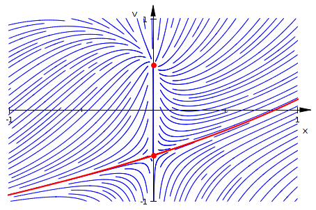
Figure 2 shows the phase portrait of the closed subsystem consisting of the first and the third equation in (8.9). One sees that the point is a saddle point and its unstable manifold (shown in red) is the graph of the first derivative to the unique solution through (the solutions for different values of are all parallel to each other and thus have the same derivative). The stable manifold is the -axis and hence irrelevant for our purposes. The point is a one-tangent node. The eigenvector again points in the -direction and thus all trajectories enter the node with a vertical tangent. This implies that none of the corresponding solutions of our second-order equation is twice differentiable at the origin.
Finally, we comment on the situation that the initial point is chosen in such a way that but . It is obvious that no strong, i. e. at least twice differentiable solution can exist in this case, as no point exists with . In principle, it was possible that in this case a unique two-sided solution existed which is everywhere smooth except at where it is only . Indeed, by our assumptions the vector field is defined everywhere on and does not vanish at such a point . Hence, there exists a unique weak generalised solution through . However, it is easy to see that it runs vertically and hence is not proper. Generally, this weak generalised solution will not run through the entire fibre, as generally for some values we will have and thus hit a point at which our above analysis applies. In this analysis, we mentioned that there are further weak generalised solutions through our singularity which are, however, not proper. One of them we have now recovered in a different manner.
9 Conclusions
We presented a geometric approach to the analysis of singular initial value problems of quasi-linear ordinary differential equations. As sketched in the first part, it is based on considering a differential equation as a submanifold of a jet bundle and using the associated contact geometry via the Vessiot spaces. We showed in the second part of this work that quasi-linear equations are special in the sense that their Vessiot distribution is projectable. This observation allows for relating the geometric singularity analysis of fully non-linear implicit equations – as e. g. discussed by Arnold [21] or Remizov [29] – with the more analytic approach to singularities of quasi-linear equations – as used e. g. by Rabier [22]. We could show in Proposition 12 that not all impasse points arising in the analysis of a quasi-linear equation stem from a singularity of the equation. Hence one indeed needs a special theory for the quasi-linear case.
In the third part of this article, we gave a detailed geometric analysis of a special class of second-order initial value problems, namely equations of the form with initial data prescribed at a simple zero of . The results represented a slight generalisation of those obtained by Liang [11] with completely different methods. In our opinion, our approach makes the appearance of a dichotomy or of a resonance and the possible existence of solutions with only finite regularity much more transparent. All these effects follow immediately from considering the phase portraits around proper impasse points at different prolongation orders. In particular, the analysis is almost automatic and requires essentially no ingenuity.
The restriction to simple zeros of is crucial for this simplicity, as it guarantees that the eigenvalue is always non-zero. Hence, even in the border case (which was ignored by Liang), we never encountered a triple eigenvalue . The situation is quite different for (generalised) Ginzburg-Landau equations of the form for some function satisfying as studied by Ignat et al. [30]. If one analyses such an equation via our approach, then one faces already in the first step the problem of studying a stationary point of a three-dimensional system where the Jacobian has a triple eigenvalue . If one succeeds here, for instance by blowing up the initial point, then the remaining analysis should be quite similar to the one presented here.
Another critical point in our approach is generally the question whether one is able to determine the eigenvalues and -vectors of all required Jacobians. For the class studied here, we obtained triagonal matrices so that this step was almost trivial posing only the problem of identifying the relevant eigenvalue. In a preliminary study of equations of the form and , i. e. of equations with a truly non-linear left hand side, it turned out that this step becomes only a little bit more difficult, but remains solvable at any prolongation order. We will present the findings for these two classes of equations elsewhere.
We assumed throughout this article that we work with smooth functions (only in Proposition 16 and in Remark 26 we considered the analytic case). In fact, almost all of our results remain true with only minor modifications, if we assume that or and , respectively, are only in for some . Obviously, we can now consider prolongations only up to order and also solutions can only be guaranteed to be in class . Thus we simply must replace smooth by .
The situation is slightly more complicated for Theorems 25 and 29. For the interesting results about finite regularity, we must assume that – in fact we should have . In the proofs we needed that the homeomorphism in the Hartman-Grobman theorem is and used the corresponding statement in [27] which, however, requires smoothness of the considered vector field. Hartman [31] showed already much earlier that the homeomorphism is under weaker conditions, namely when the linear part defines a contraction and the non-linear part has uniformly Lipschitz continuous partial derivatives. We applied the Hartman-Grobman theorem to the vector field around the stationary point . According to (8.3), the field depends on which by (8.2) is obtained by differentiating times . If , then is still at least of class and thus the coefficients of possess the required regularity. For the contraction property, we recall that the Jacobian of the reduced dynamics has the eigenvalues and thus defines a contraction, if and only if . We may perform a rescaling of the independent variable . Then a simple computation shows that the parameters and rescale according to and . Thus the resonance condition is not affected by the rescaling, but we may assume without loss of generality that so that Hartman’s result can be applied.
A referee pointed out that the resonance condition in the here considered second-order initial value problem could be derived for analytic equations via the Newton-Puiseux construction of Cano [15]. This observation represents an interesting question for future research. For the class of problems considered here, it was straightforward to derive the conditions both for the dichotomy of the existence theory and for the resonances. For other initial value problems, this is no longer the case and the combination of our geometric techniques with such algebraic approaches may prove very useful here.
Acknowledgements
It is a pleasure for us to thank Sebastian Walcher (RWTH Aachen) and Peter de Maesschalck (Hasselt University) for helpful discussions about the theory of dynamical systems. Oscar Saleta Reig (Universitat Autònoma de Barcelona) helped us with using P4. We also appreciate the useful comments of an anonymous referee. This work was supported by the bilateral project ANR-17-CE40-0036 and DFG-391322026 SYMBIONT.
References
- [1] V. Arnold, S. Gusejn-Zade, A. Varchenko, Singularities of Differentiable Maps I: The Classification of Critical Points, Caustics and Wave Fronts, Monographs in Mathematics 82, Birkhäuser, Boston, 1985.
- [2] M. Golubitsky, V. Guillemin, Stable Mappings and Their Singularities, Graduate Texts in Mathematics 14, Springer-Verlag, New York, 1973.
- [3] L. Dara, Singularités génériques des équations différentielles multiformes, Bol. Soc. Bras. Mat. 6 (1975) 95–128.
- [4] A. Davydov, G. Ishikawa, S. Izumiya, W.-Z. Sun, Generic singularities of implicit systems of first order differential equations on the plane, Japan. J. Math. 3 (2008) 93–119.
- [5] P. Rabier, W. Rheinboldt, Theoretical and numerical analysis of differential-algebraic equations, in: P. Ciarlet, J. Lions (Eds.), Handbook of Numerical Analysis, Vol. VIII, North-Holland, Amsterdam, 2002, pp. 183–540.
- [6] R. Riaza, Differential-Algebraic Systems, World Scientific, Hackensack, 2008.
- [7] G. Thomas, The problem of defining the singular points of quasi-linear differential-algebraic systems, Theor. Comp. Sci. 187 (1997) 49–79.
- [8] J. Tuomela, On singular points of quasilinear differential and differential-algebraic equations, BIT 37 (1997) 968–977.
- [9] W. Seiler, Singularities of implicit differential equations and static bifurcations, in: V. Gerdt, W. Koepf, E. Mayr, E. Vorozhtsov (Eds.), Computer Algebra in Scientific Computing — CASC 2013, Lecture Notes in Computer Science 8136, Springer-Verlag, Cham, 2013, pp. 355–368.
- [10] F. Dumortier, J. Llibre, J. Artés, Qualitative Theory of Planar Differential Systems, Universitext, Springer-Verlag, Berlin, 2006.
- [11] J. Liang, A singular initial value problem and self-similar solutions of a nonlinear dissipative wave equation, J. Diff. Eqs. 246 (2009) 819–844.
- [12] H. Fine, On the functions defined by differential equations, with an extension of the Puiseux polygon construction to these equations, Amer. J. Math. 11 (1889) 317–328.
- [13] H. Fine, Singular solutions of ordinary differential equations, Amer. J. Math. 12 (1890) 295–322.
- [14] A. Bruno, Local Methods in Nonlinear Differential Equations, Springer-Verlag, Berlin, 1989.
- [15] J. Cano, On the series defined by a differential equations, with an extension of the Puiseux polygon construction to these equations, Analysis 13 (1993) 103–120.
- [16] S. Falkensteiner, Power series solutions of AODEs — existence, uniqueness, convergence and computation, Ph.D. thesis, Universität Linz, Linz (2020).
- [17] M. Lange-Hegermann, D. Robertz, W. Seiler, M. Seiß, Singularities of algebraic differential equations, Preprint Kassel University (arXiv:2002.11597) (2020).
- [18] D. Saunders, The Geometry of Jet Bundles, London Mathematical Society Lecture Notes Series 142, Cambridge University Press, Cambridge, 1989.
- [19] W. Seiler, Involution — The Formal Theory of Differential Equations and its Applications in Computer Algebra, Algorithms and Computation in Mathematics 24, Springer-Verlag, Berlin, 2010.
- [20] W. Seiler, M. Seiß, Algebraic and geometric analysis of singularities of implicit differential equations, in: F. Boulier, M. England, T. Sadykov, E. Vorozhtsov (Eds.), Computer Algebra and Scientific Computing — CASC 2020, Lecture Notes in Computer Science, Springer-Verlag, Cham, 2020, accepted for publication.
- [21] V. Arnold, Geometrical Methods in the Theory of Ordinary Differential Equations, Edition, Grundlehren der mathematischen Wissenschaften 250, Springer-Verlag, New York, 1988.
- [22] P. Rabier, Implicit differential equations near a singular point, J. Math. Anal. Appl. 144 (1989) 425–449.
- [23] U. Kant, W. Seiler, Singularities in the geometric theory of differential equations, in: W. Feng, Z. Feng, M. Grasselli, X. Lu, S. Siegmund, J. Voigt (Eds.), Dynamical Systems, Differential Equations and Applications (Proc. 8th AIMS Conference, Dresden 2010), Vol. 2, AIMS, 2012, pp. 784–793.
- [24] L. Perko, Differential Equations and Dynamical Systems, 3rd Edition, Texts in Applied Mathematics 7, Springer-Verlag, 2001.
- [25] J. Sijbrand, Properties of center manifolds, Trans. AMS 289 (1985) 431–469.
- [26] J. Guckenheimer, P. Holmes, Nonlinear Oscillations, Dynamical Systems, and Bifurcations of Vector Fields, Applied Mathematical Sciences 42, Springer-Verlag, New York, 1990.
- [27] M. Guysinsky, B. Hasselblatt, V. Rayskin, Differentiability of the Hartman-Grobman linearization, Discr. Cont. Dyn. Sys. 9 (2003) 979–984.
- [28] R. Fiorenza, Hölder and locally Hölder Continuous Functions, and Open Sets of Class , , Frontiers in Mathematics, Birkhäuser, Cham, 2016.
- [29] A. Remizov, Multidimensional Poincaré construction and singularities of lifted fields for implicit differential equations, J. Math. Sci. 151 (2008) 3561–3602.
- [30] R. Ignat, L. Nguyen, V. Slastikov, A. Zarnescu, Uniqueness results for an ODE related to a generalized Ginzburg-Landau model for liquid crystals, SIAM J. Math. Anal. 46 (2014) 3390–3425.
- [31] P. Hartman, On local homeomorphisms of Euclidean spaces, Bol. Soc. Mat. Mex. 5 (1960) 220–241.