Learning Not to Learn in the Presence of Noisy Labels
Abstract
Learning in the presence of label noise is a challenging yet important task: it is crucial to design models that are robust in the presence of mislabeled datasets. In this paper, we discover that a new class of loss functions called the gambler’s loss provides strong robustness to label noise across various levels of corruption. We show that training with this loss function encourages the model to “abstain” from learning on the data points with noisy labels, resulting in a simple and effective method to improve robustness and generalization. In addition, we propose two practical extensions of the method: 1) an analytical early stopping criterion to approximately stop training before the memorization of noisy labels, as well as 2) a heuristic for setting hyperparameters which do not require knowledge of the noise corruption rate. We demonstrate the effectiveness of our method by achieving strong results across three image and text classification tasks as compared to existing baselines.
Keywords:
Machine Learning, ICML1 Introduction
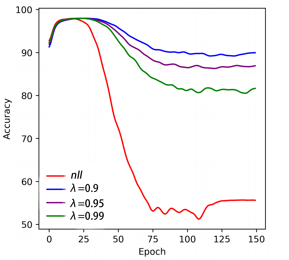
Learning representations from real-world data can greatly benefit from clean annotation labels. However, real-world data can often be mislabeled due to 1) annotator mistakes as a natural consequence of large-scale crowdsourcing procedures (Howe 2008), 2) the difficulty in fine-grained labeling across a wide range of possible labels (Russakovsky et al. 2015), 3) subjective differences when annotating emotional content (Busso et al. 2008), and 4) the use of large-scale weak supervision (Dehghani et al. 2017). Learning in the presence of noisy labels is challenging since overparametrized neural networks are known to be able to memorize both clean and noisy labels even with strong regularization (Zhang et al. 2017). Empirical results have shown that when the model memorizes noisy labels, its generalization performance on test data deteriorates (e.g., see Figure 4). Therefore, learning in the presence of label noise is a challenging yet important task: it is crucial to design models that are robust in the presence of mislabeled datasets.
In this paper, we show that a new class of loss functions called the gambler’s loss (Ziyin et al. 2019) provides strong robustness to label noise across various levels of corruption. We start with a theoretical analysis of the learning dynamics of this loss function and demonstrate through extensive experiments that it is robust to noisy labels. Our theory also motivates for two practical extensions of the method: 1) an analytical early stopping criterion designed to stop training before memorization of noisy labels, and 2) a training heuristic that relieves the need for hyperparameter tuning and works well without requiring knowledge of the noise corruption rate. Finally, we show that the proposed method achieves state-of-the-art results across three image (MNIST, CIFAR-10) and text (IMDB) classification tasks, compared to prior algorithms.
2 Background and Related Work
In this section we review important background and prior work related to our paper.
Label Noise: Modern datasets often contain a lot of labeling errors (Russakovsky et al. 2015; Schroff et al. 2010). Two common approaches to deal with noisy labels involve using a surrogate loss function (Patrini et al. 2017; Zhang & Sabuncu 2018; Xu et al. 2019) that is specific to the label noise problem at hand, or designing a special training scheme to alleviate the negative effect of learning from data points with wrong labels (Yu et al. 2019). In this work, we mainly compare with the following two recent state-of-the-art methods: Co-teaching+ (Yu et al. 2019): this method simultaneously trains two networks which update each other with the other’s predicted label to decouple the mistakes; Generalized cross-entropy () (Zhang & Sabuncu 2018): this method uses a loss function that incorporates the noise-robust properties of MAE (mean absolute error) while retaining the training advantages of CCE (categorical cross-entropy).
Early Stopping. Early stopping is an old problem in machine learning (Prechelt 1998; Amari 1998), but studying it in the context of label noise appeared only recently (Li et al. 2019; Hu et al. 2019). It has been shown theoretically (Li et al. 2019) that early stopping can constitute an effective way to defend against label noise, but no concrete method or heuristic has been presented. In this paper, we propose an early stopping method that can be used jointly with the gambler’s loss function. Our analysis on this loss function allows us to propose an analytic function to predict an early stopping threshold without using a validation set and is independent of the model and the task, provided that the model has sufficient complexity to solve the task (e.g. overparametrized neural networks). To the best of our knowledge, we have proposed the first early stopping method effective for noise labels.
Learning to Abstain: Within the paradigm of selective classification, a model aims to abstain from making predictions at test time in order to achieve higher prediction accuracy (El-Yaniv & Wiener 2010). Given a -class prediction function and a selection function , a selective classifier can be defined as
| (1) |
Efforts to optimize such a classifier have evolved from a method to train given an existing trained to a multi-headed model architecture that jointly trains and given the desired fraction of data points (Geifman & El-Yaniv 2019). The gambler’s loss represents a recent advancement in this area by jointly training by modifying the loss function and thus introducing a more versatile selective classifier that performs at the SOTA (Ziyin et al. 2019).
2.1 Gambler’s Loss Function
The gambler’s loss draws on the analogy of a classification problem as a horse race with bet and reserve strategies. Reserving from making a bet in a gamble can be seen as a machine learning model abstaining from making a prediction when uncertain. This background on gambling strategies has been well studied and motivated in the information theory literature (Cover & Thomas 2006; Cover 1991), and was recently connected to prediction in the machine learning literature (Ziyin et al. 2019).
We provide a short review but defer the reader to Ziyin et al. 2019 for details. An -class classification task is defined as finding a function , where is the input dimension, is the number of classes, and denotes the parameters of . We assume that the output is normalized, and can be seen as the predicted probability of input being labeled in class , i.e. and our goal is to maximize the log probability of the true label :
| (2) |
The gambler’s loss involves adding an output neuron at the “-th dimension” to function as an abstention, or rejection, score. The new model, augmented with the rejection score, is trained through the gambler’s loss function:
| (3) |
where is the hyperparameter of the loss function, interpolating between the cross-entropy loss and the gambler’s loss and controlling the incentive for the model to abstain from prediction, with higher encouraging abstention. It is shown that the augmented model learns to output abstention score that correlates well with the uncertainty about the input data point , either when the data point has inherent uncertainty (i.e. its true label is not a delta function), or when is an out-of-distribution sample. This work studies the dynamic training aspects of the gambler’s loss and utilizing these properties to pioneer a series of techniques that are robust in the presence of label noise. In particular, we argue that the gambler’s loss is a noise-robust loss function.
3 Gambler’s Loss is Robust to Label Noise
In this section, we examine binary classification problems in the presence of noisy labels. We begin by defining a bias-variance trade-off for learning with noisy labels (section 3.1) and showing that the gambler’s loss reduces generalization error (section 3.2). Corroborated by the theory, we demonstrate three main effects of training with gambler’s loss: 1) the gambler’s loss automatically prunes part of the dataset (Figure 1); 2) the gambler’s loss can differentiate between training data that is mislabeled and data that is cleanly labeled (Figure 3); and 3) lower can improve generalization performance (Figure 3). These theoretical and empirical findings suggest that training with the gambler’s loss improves learning from noisy labels.
3.1 Bias-Variance Trade-off in Noisy Classification
The bias-variance trade-off is universal; it has been discovered in the regression setting that it plays a central role in understanding learning in the presence of label noise (Krogh & Hertz 1992a; Krogh & Hertz 1992b; Hastie et al. 2019). We first show that the loss function we are studying can be decomposed into generalized bias and variance terms; this suggests that, as in a regression problem, we might introduce regularization terms to improve generalization.
This section sets the notation and presents background for our theoretical analysis. Consider a learning task with input-targets pairs forming the test set. We assume that are drawn i.i.d. from a joint distribution . We also assume that for any given , can be uniquely determined, so that . We also assume that the distribution of two classes are balanced, i.e. . We denote model outputs as . The empirical generalization error is defined as
which is the cross-entropy loss on the empirical test set. We assume that our model converges to the global minimum of the training objective since it has been proved that neural networks can find the global minimum easily (Du et al. 2018).
However, a problem with the binary label is that diverges and the loss function diverges when a point is mislabeled, rendering the cross-entropy loss (also called loss) very hard to analyze. To deal with this problem, we replace the binary label by slightly smoothed version , where is the smoothing parameter and is perturbatively small (Szegedy et al. 2016). We will later take the limit to make our analysis independent of the artificial smoothing we introduced. The optimal solution in this case is simply , where the generalization error converges to
| (4) |
as , the generalization error converges to .
Now, we assume that label noise is present in the dataset such that each label is flipped to the other label with probability , we assume that . We define to be the corruption rate and to be the clean rate. The generalization error of our training dataset becomes
| (5) | ||||
| (6) | ||||
| (7) | ||||
| (8) |
where denotes the new set of perturbed labels. Therefore, we have partitioned the original loss function into two separate loss functions, where is the loss for the data points whose original label is , and likewise for . The global optimum, as , for is , the entropy of . The generalization error of this solution is
| (9) |
where we have taken expectations over the noise. We observe a bias-variance trade-off, where the first term denotes the variance in the original labels, while the second term is the bias introduced due to noise. As , the noise disappears and we achieve perfect generalization where the training loss is the same as generalization loss.


3.2 Training and Robustness with the Gambler’s Loss
The gambler’s loss function was proposed by Ziyin et al. 2019 as a training method to learn an abstention mechanism. We propose to train, instead of on equation (5), but rather on the gambler’s loss with hyperparameter :
| (10) | ||||
| (11) |
where we have rewritten and , and we have augmented the model with one more output dimension denoting the rejection score. Notice that the gambler’s loss requires the normalization condition:
| (12) |

To proceed, we define learnability on a data point from the perspective of gambler’s loss. We note that this definition is different but can be related to standard PAC-learnability (Shalev-Shwartz & Ben-David 2014).
Definition 3.1.
A data point is said to be not learnable if the optimal solution on the gambler’s loss of such point outputs . Otherwise, the point is learnable.
Since one category always predicts , this prediction saturates the softmax layer of a neural network, making further learning on such a data point impossible as the gradient vanishes. If a model predicts as a rejection score, then it will abstain from assigning weight to any of the classes, thus avoiding learning from data point completely.
We now show that, when , then the points with are not learnable.
Theorem 3.1.
For a point , with label (assuming ) where denotes the probability that , and if then the optimal solution to the loss function
is given by
with , i.e. the model will predict on both classes.
See Appendix A for the proof. Note that is roughly of similar magnitude to the entropy of given . Therefore, if we want to prune part of the dataset that appears “random”, we can choose to be smaller than the entropy of that part of the dataset. To be more insightful, we have a control over the model complexity:
Corollary 3.1.1.
Let be the subset of the dataset that are learnable at hyperparameter , and let be the optimal model trained on using cross-entropy loss, then .
This result implies that the model will not learn part of the dataset if it appears too random. See Figure 1 for a demonstration of this effect, we see that training with the classical nll loss memorizes all the data points at convergence, while gambler’s loss selectively learns only , resulting in a absolute performance improvement at testing.
The following theorem gives an expression for what an optimal model would predict for the learnable points.
Theorem 3.2.
Let , then the optimal solution to a learnable point , whose label is and , is
| (13) |
This says that the optimal model will make the following prediction learnable point , where :
| (14) |
By combining Theorem 3.1 and Theorem 3.2, we observe that the model will predict a higher rejection score on the mislabeled points (close to , since their conditional entropy is large), and lower rejection score on the correctly labeled data points (since their conditional entropy is small) in the training set. This is exactly what we observe in Figure 3, where we plot the rejection scores on both clean and corrupted portions of the dataset, with noise corruption rates ranging from to . We observe that our model learns rejection scores smaller than for data points with clean labels and learns larger rejection score for data points with corrupted labels. In other words, we are able to approximately filter out the corrupted labels which can then be sent for relabeling in real-world scenarios.


Since generalization error is reduced by training with the gambler’s loss, we conclude that the gambler’s loss is robust to the presence of noisy labels on learnable points.
Theorem 3.3.
Let be the generalization error achieved by the global minimum by the Kullbeck-Leibler’s divergence with smoothing parameter and corruption rate , given by equation (9), and let be the generalization error achieved by training on the gambler’s loss, where we make the prediction on each data point. Then,
| (15) |
for and . The equality is achieved when , i.e., when no noise is present.
Proof is given in Appendix C. This shows that whenever noise is present, using gambler’s loss will achieve better generalization than training using loss, even if we are not aware of the corruption rate. Figure 3 shows that lower indeed results in better generalization in the presence of label noise. In addition, results in Table 2 show that training with gambler’s loss can improve over loss when corruption is present.
4 Practical Extensions
While using the gambler’s loss in isolation already gives strong theoretical guarantees and empirical performance in noisy label settings, we propose two practical extensions that further improve performance. The first is an analytical early stopping criterion that is designed to stop training before the memorization of noisy labels begins and hurts generalization. The second is a training heuristic that relieves the need for hyperparameter tuning and works well without requiring knowledge of the noise corruption rate.
4.1 An Early Stopping Criterion


We further propose an analytical early stopping criterion that allows us to perform early stopping with label noise without a validation set. We begin by rewriting the generalization error we derived in equation (8) as a function of :
| (16) | ||||
| (17) | ||||
| (18) | ||||
| (19) |
where, in the last line, we make a “mean-field” assumption that the effect of the noise can be averaged over and replaced by the expected value of the indicators. This mean-field assumption is reasonable because it has been shown that learning in neural networks often proceeds at different stages, first learning low complexity functions and then proceeding to learn functions of higher complexity, with a random function being the most complex (Nakkiran et al. 2019). Thus, while learning the simpler function of true features, we can understand the effect in a mean-field manner. We argue the validity of this assumption lies in its capability of predicting the point of early stopping accurately and thereby improving performance. We use the upper-bar mark to denote this mean-field solution (i.e. ) and apply the same approximation to , yielding .
Let denote the clean rate, we can derive an expression for the effective loss function as follows:
Theorem 4.1.
The mean-field gambler’s loss takes the form:
| (20) |
which exhibits an optimal solution at training loss
| (21) | ||||
| (22) |
which depends only on and .
The proof is given in Appendix D. Notice that this result extends directly without modification to the case of multiclass classification. Since the proof involves dealing with separately, and, as more classes are added, we only add terms such as and so on. When , the mean-field solution is greater than , the global minimum, and this has the important implication that, when learning in the presence of label noise, a semi-stable solution at exists, and is exhibited in the learning trajectory as a plateau around . After this plateau, the loss gradually converges to the global minimum at training loss. We refer to these three regimes with learning in the presence of noise as:
1) Fast Learning Stage: The model quickly learns the underlying mapping from data to clean labels; one observes rapid decrease in training loss and increases in test accuracy.
2) Gap Stage: This is the stage where the mean-field solution holds approximately. From Figure 4(a), learning on the clean labels is almost complete () but training on noisy labels has not started yet (), and a large gap in training loss exists between the clean and corrupt part of the training set. Both the training loss and the test accuracy reach a plateau, and this is the time at which the generalization performance is the best.
3) Memorization: This refers to the last regime when the model memorizes these noisy labels and the train loss decreases slowly to .
In addition to providing insights on the training trajectories in the presence of noisy labels, Theorem 4.1 also tells us that a network trained with the gambler’s loss function with hyperparameter on a symmetrically corrupted dataset with corruption rate should have training loss around during the gap stage, where generalization is the best. This motivates using as an early stopping criterion. From the training plots in Figure 5, we see that the plateaus we hypothesize do indeed exist and our early stopping criterion accurately estimates the height of the plateau, thereby predicting close to the optimal early stopping point. In comparison with the standard early stopping technique by monitoring accuracy/loss on a validation set, we show that our proposed early stopping method is more accurate (Section 5.1).
| large | small | |
| learning speed | ||
| robustness |
4.2 A Heuristic for Scheduling Automatically
| Dataset | nll loss | requires corruption rate | agnostic to corruption rate | |||
| Coteaching+ | Gamblers (AES) | Loss | Gamblers | Gamblers + schedule | ||
| MNIST | ||||||
| MNIST | ||||||
| MNIST | ||||||
| MNIST | ||||||
| IMDB | ||||||
| IMDB | ||||||
| IMDB | ||||||
| IMDB | ||||||
| CIFAR10 | ||||||
| CIFAR10 | ||||||
| CIFAR10 | ||||||
| CIFAR10 | ||||||
| Dataset | VES | Gamblers AES |
| MN | ||
| MN | ||
| MN | ||
| MN | ||
| IMDB | ||
| IMDB | ||
| IMDB |
While the above section presents an effective guideline for early stopping in the presence label noise, it still requires tuning the hyperparameter . In practice, choosing for the optimal is not straightforward and requires special tuning for different tasks. In this section, we present a heuristic that eliminates the need for tuning . It also carries the important benefit of not requiring knowledge of the label corruption rate.
This section is based on the gambling analogy (Cover & Thomas 2006; Markowitz 1952; Cover 1991) and the following two properties of training on gambler’s loss: (1) larger encourages feature learning and smaller slows down learning (Ziyin et al. 2019); (2) smaller encourages robustness and larger provides less robustness (this paper). This means that there is a trade-off between the speed of feature learning and robustness when using gambler’s loss. As a result, it would be ideal to balance both aspects and set to achieve a better trade-off between robustness and feature learning. See Table 1 for a summary of these trade-offs.
Recall that for true label , the gambler’s loss is given by
| (23) |
This loss can decrease in two ways: (1) (trivial learning) one may trivially decrease the loss by increasing which is the rejection score. Since is present in every category, this does not correspond to learning; (2) one may increase the output on the true label , which corresponds to actual learning. While lower gives better robustness to label noise, it also encourages trivial learning. In fact, as shown in Theorem 3.1, choosing too small leads to a trivial solution with a loss of . Therefore, one is motivated to choose the lowest such that normal learning can still occur. More importantly, since different data points are learned at potentially different speeds (Bengio et al. 2009), we propose a rule to automatically set adaptively as a function of each data point (rather than a general ). For a data point , let denote the predicted probability. We choose to be
| (24) |
Firstly, as a sanity check, the Cauchy-Schwarz inequality tells us that , which is in the well-defined range for gambler’s loss. The choice for in equation (24) comes from the fact that we can view the classification problem as a horse race betting problem. In the gambler’s loss analogy, represents the return on a correct bet (Ziyin et al. 2019). As the model trains, the optimal will tend to decrease as the model gains confidence on the data in the training set and is less likely to resort to trivial learning. Thus, intuitively, we would like to decrease as the model grows more confident. To achieve this, we examine the gain of the gambler from a single round of betting:
| (25) |
where we write for concision. Greater model confidence corresponds to greater expected gain on the part of the gambler since the gambler will consolidate bets on certain classes as certainty increases. Therefore, to achieve a appropriate for the current gain, we set such that the expected gain of the gambler is constant. Since our metaphorical starts with units of currency to gamble, we naturally choose as our constant:
| (26) |
To the gambler, the only unknown is , but we can recover the gambler’s expectation through his bets: . Thus, we obtain:
| (27) |
In section 5.2, we extensively study the performance of automatic scheduling using and we show that it achieves SOTA results on three datasets.
In Appendix E, we derive and discuss an alternative scheduling rule by directly setting the doubling rate (i.e. the loss function we are optimizing over) to (i.e. its minimum value). This gives us
| (28) |
By Jensen’s inequality,
| (29) |
showing that encourages learning more at the expense of robustness. If better training speed is desired, we expect to perform better. While our experiments focus on showcasing the effectiveness of , we discuss the performance of both strategies in Appendix E.
5 Benchmark Experiments
In this section, we experiment with the proposed methods under standard label noise settings. We first show that our proposed early stopping criterion (section 4.1) stops at a better point as compared to classical early stopping methods based on validation sets. Next, we show that dynamic scheduling using (section 4.2) achieves state-of-the-art results as compared to existing baselines.
5.1 Early Stopping Criterion
We split images from the training set to make a validation set, and we early stop when the validation accuracy stops to increase for consecutive epochs. There are also a few other validation-based early stopping criteria, but they are shown to perform similarly (Prechelt 1998). We refer to early stopping techniques based on monitoring the validation loss as VES (validation early stopping) and call our method AES (analytical early stopping). We fix when training our models and collect the results in Table 3. On MNIST, we see that our proposed method significantly outperforms the baseline early stopping methods both by testing performance (up to in absolute accuracy) and training time ( times faster); We also conduct experiments on the IMDB dataset (Maas et al. 2011), which is a standard NLP sentiment analysis binary classification task. We use a standard LSTM with a hidden dimension of and -dimensional pretrained GloVe word embeddings (Pennington et al. 2014). Again, we notice that AES consistently improves on early stopping on a validation set (by about in absolute accuracy). We hypothesize that the small sizes of the validation set result in a large variance of the early stopping estimates. This problem becomes more serious when label noise is present. On the other hand, AES does not require estimation on a small validation set and is more accurate for early stopping.
5.2 Automatic Scheduling
In this section, we demonstrate that the proposed scheduling method achieves very strong performance when compared to other benchmarks, which include the generalized cross-entropy loss () (Zhang & Sabuncu 2018) and Coteaching+ (Yu et al. 2019). Generalized cross-entropy loss serves as a direct comparison to our scheduling method: it is the current SOTA method for noisy label classification that is agnostic to the corruption rate and modifies only the loss function, two qualities shared by our method. We set the hyperparameter for following the experiments in (Zhang & Sabuncu 2018). Meanwhile, Coteaching+, the SOTA method when the corruption rate is known, introduces a novel data pruning method. In our comparison, we give Coteaching+ the true corruption rate , but we note that its performance is likely to drop when is unknown and has to be estimated beforehand. We perform experiments on datasets, ranging from standard image classification tasks (MNIST: class; CIFAR-10: class) to text classification tasks using LSTM with attention and pretrained GloVe word embedding (IMDB: class). For the IMDB dataset, we use the LaProp optimizer (Ziyin et al. 2020). We note that training with LaProp is faster and stabler than using Adam (Kingma & Ba 2014).
From the results in Table 2, we see that automatic scheduling outperforms in out of categories in a statistically significant way. More importantly, we see larger margins of improvement as the noise rate increases. is only better than scheduled gambler’s loss on MNIST at the lowest corruption rate () and only by accuracy. Furthermore, the scheduled gambler’s loss also outperforms Coteaching+ on 2 out of 3 datasets we compare on ( categories out of ), while using only one half of the training time and not requiring knowledge of the true corruption rate. For CIFAR-10 and MNIST, the gambler’s loss is especially strong when the noise rate is extreme. For example, when , the scheduled gambler’s loss significantly outperforms Coteaching+ by in absolute accuracy on MNIST, and by in absolute accuracy on CIFAR-10.
6 Conclusion
In this paper, we demonstrated how a theoretically motivated study of learning dynamics translates directly to the invention of new effective algorithms. In particular, we showed that the gambler’s loss function features a unique training trajectory that makes it particularly suitable for robust learning from noisy labels and improving the generalization of existing classifications models. We also presented two practical extensions of the gambler’s loss that further increase its effectiveness in combating label noise: (1) an early stopping criterion that can be used to accelerate training and improve generalization when the corruption rate is known, and (2) a heuristic for setting hyperparameters which does not require knowledge of the noise corruption rate. Our proposed methods achieve the state-of-the-art results on three datasets when compared to existing label noise methods.
References
- Amari (1998) Amari, S.-I. Natural gradient works efficiently in learning. Neural Comput., 10(2):251–276, February 1998. ISSN 0899-7667. doi: 10.1162/089976698300017746. URL http://dx.doi.org/10.1162/089976698300017746.
- Bengio et al. (2009) Bengio, Y., Louradour, J., Collobert, R., and Weston, J. Curriculum learning. In Proceedings of the 26th Annual International Conference on Machine Learning, ICML ’09, pp. 41–48, New York, NY, USA, 2009. Association for Computing Machinery. ISBN 9781605585161. doi: 10.1145/1553374.1553380. URL https://doi.org/10.1145/1553374.1553380.
- Busso et al. (2008) Busso, C., Bulut, M., Lee, C.-C., Kazemzadeh, A., Mower, E., Kim, S., Chang, J. N., Lee, S., and Narayanan, S. Iemocap: interactive emotional dyadic motion capture database. Language Resources and Evaluation, 42(4):335–359, 2008. URL http://dblp.uni-trier.de/db/journals/lre/lre42.html#BussoBLKMKCLN08.
- Cover (1991) Cover, T. M. Universal portfolios. Mathematical Finance, 1(1):1–29, 1991. doi: 10.1111/j.1467-9965.1991.tb00002.x. URL https://onlinelibrary.wiley.com/doi/abs/10.1111/j.1467-9965.1991.tb00002.x.
- Cover & Thomas (2006) Cover, T. M. and Thomas, J. A. Elements of Information Theory (Wiley Series in Telecommunications and Signal Processing). Wiley-Interscience, New York, NY, USA, 2006. ISBN 0471241954.
- Dehghani et al. (2017) Dehghani, M., Severyn, A., Rothe, S., and Kamps, J. Avoiding your teacher’s mistakes: Training neural networks with controlled weak supervision. In arXiv, 2017. URL https://arxiv.org/abs/1711.00313.
- Du et al. (2018) Du, S. S., Lee, J. D., Li, H., Wang, L., and Zhai, X. Gradient descent finds global minima of deep neural networks. arXiv preprint arXiv:1811.03804, 2018.
- El-Yaniv & Wiener (2010) El-Yaniv, R. and Wiener, Y. On the foundations of noise-free selective classification. Journal of Machine Learning Research, 11(May):1605–1641, 2010.
- Geifman & El-Yaniv (2019) Geifman, Y. and El-Yaniv, R. Selectivenet: A deep neural network with an integrated reject option. arXiv preprint arXiv:1901.09192, 2019.
- Hastie et al. (2019) Hastie, T., Montanari, A., Rosset, S., and Tibshirani, R. J. Surprises in high-dimensional ridgeless least squares interpolation. arXiv preprint arXiv:1903.08560, 2019.
- Howe (2008) Howe, J. Crowdsourcing: Why the Power of the Crowd Is Driving the Future of Business. Crown Publishing Group, New York, NY, USA, 1 edition, 2008. ISBN 0307396207, 9780307396204.
- Hu et al. (2019) Hu, W., Li, Z., and Yu, D. Understanding generalization of deep neural networks trained with noisy labels. arXiv preprint arXiv:1905.11368, 2019.
- Kingma & Ba (2014) Kingma, D. P. and Ba, J. Adam: A method for stochastic optimization. CoRR, abs/1412.6980, 2014. URL http://dblp.uni-trier.de/db/journals/corr/corr1412.html#KingmaB14.
- Krogh & Hertz (1992a) Krogh, A. and Hertz, J. A. Generalization in a linear perceptron in the presence of noise. Journal of Physics A: Mathematical and General, 25(5):1135, 1992a.
- Krogh & Hertz (1992b) Krogh, A. and Hertz, J. A. A simple weight decay can improve generalization. In Advances in neural information processing systems, pp. 950–957, 1992b.
- Li et al. (2019) Li, M., Soltanolkotabi, M., and Oymak, S. Gradient descent with early stopping is provably robust to label noise for overparameterized neural networks. arXiv preprint arXiv:1903.11680, 2019.
- Maas et al. (2011) Maas, A. L., Daly, R. E., Pham, P. T., Huang, D., Ng, A. Y., and Potts, C. Learning word vectors for sentiment analysis. In Proceedings of the 49th Annual Meeting of the Association for Computational Linguistics: Human Language Technologies, pp. 142–150, Portland, Oregon, USA, June 2011. Association for Computational Linguistics. URL http://www.aclweb.org/anthology/P11-1015.
- Markowitz (1952) Markowitz, H. Portfolio selection. The Journal of Finance, 7(1):77–91, 1952. ISSN 00221082, 15406261. URL http://www.jstor.org/stable/2975974.
- Nakkiran et al. (2019) Nakkiran, P., Kaplun, G., Kalimeris, D., Yang, T., Edelman, B. L., Zhang, F., and Barak, B. Sgd on neural networks learns functions of increasing complexity. arXiv preprint arXiv:1905.11604, 2019.
- Patrini et al. (2017) Patrini, G., Rozza, A., Krishna Menon, A., Nock, R., and Qu, L. Making deep neural networks robust to label noise: A loss correction approach. In Proceedings of the IEEE Conference on Computer Vision and Pattern Recognition, pp. 1944–1952, 2017.
- Pennington et al. (2014) Pennington, J., Socher, R., and Manning, C. Glove: Global vectors for word representation. In Proceedings of the 2014 conference on empirical methods in natural language processing (EMNLP), pp. 1532–1543, 2014.
- Prechelt (1998) Prechelt, L. Early stopping-but when? In Neural Networks: Tricks of the trade, pp. 55–69. Springer, 1998.
- Russakovsky et al. (2015) Russakovsky, O., Deng, J., Su, H., Krause, J., Satheesh, S., Ma, S., Huang, Z., Karpathy, A., Khosla, A., Bernstein, M., et al. Imagenet large scale visual recognition challenge. International journal of computer vision, 115(3):211–252, 2015.
- Schroff et al. (2010) Schroff, F., Criminisi, A., and Zisserman, A. Harvesting image databases from the web. IEEE transactions on pattern analysis and machine intelligence, 33(4):754–766, 2010.
- Shalev-Shwartz & Ben-David (2014) Shalev-Shwartz, S. and Ben-David, S. Understanding machine learning: From theory to algorithms. Cambridge university press, 2014.
- Szegedy et al. (2016) Szegedy, C., Vanhoucke, V., Ioffe, S., Shlens, J., and Wojna, Z. Rethinking the inception architecture for computer vision. In Proceedings of IEEE Conference on Computer Vision and Pattern Recognition,, 2016. URL http://arxiv.org/abs/1512.00567.
- Xu et al. (2019) Xu, Y., Cao, P., Kong, Y., and Wang, Y. L_dmi: An information-theoretic noise-robust loss function. arXiv preprint arXiv:1909.03388, 2019.
- Yu et al. (2019) Yu, X., Han, B., Yao, J., Niu, G., Tsang, I., and Sugiyama, M. How does disagreement help generalization against label corruption? In International Conference on Machine Learning, pp. 7164–7173, 2019.
- Zhang et al. (2017) Zhang, C., Bengio, S., Hardt, M., Recht, B., and Vinyals, O. Understanding deep learning requires rethinking generalization. ArXiv e-prints, 2017. URL https://arxiv.org/abs/1611.03530.
- Zhang & Sabuncu (2018) Zhang, Z. and Sabuncu, M. Generalized cross entropy loss for training deep neural networks with noisy labels. In Advances in neural information processing systems, pp. 8778–8788, 2018.
- Ziyin et al. (2019) Ziyin, L., Wang, Z., Liang, P. P., Salakhutdinov, R. R., Morency, L.-P., and Ueda, M. Deep gamblers: Learning to abstain with portfolio theory. In Wallach, H., Larochelle, H., Beygelzimer, A., d'Alché-Buc, F., Fox, E., and Garnett, R. (eds.), Advances in Neural Information Processing Systems 32, pp. 10622–10632. Curran Associates, Inc., 2019. URL http://papers.nips.cc/paper/9247-deep-gamblers-learning-to-abstain-with-portfolio-theory.pdf.
- Ziyin et al. (2020) Ziyin, L., Wang, Z. T., and Ueda, M. Laprop: a better way to combine momentum with adaptive gradient. arXiv preprint arXiv:2002.04839, 2020.
Appendix A Proof of Theorem 3.1 and Theorem 3.2
Taking the gambler’s analogy, this theorem simply means that a gambler betting randomly will not make money, and so the better strategy is to reserve money in the pocket. Let be the gambler’s hyperparameter. Let be the predicted probability on the true label , and let denote the prediction made on all the wrong classes added altogether, be the predicted confidence score by the gambler’s loss. By definition of a probability distribution, we have .
We first show that . Intuitively speaking, this simply means that a gambler betting randomly will not make money, and so the better strategy is to reserve money in the pocket, and so it suffices to show that for any solution , the solution achieves better or equal doubling rate. For a mislabeled point (we drop ), the loss is but , and so , and we have that optimal solution always have .
Now, we find the optimal solution to
| (30) |
by taking the derivative with respect to p:
| (31) |
and then setting it equal to 0
| (32) |
is the :
| (33) |
and notice that if .
Appendix B Proof of Corollary 3.1.1
Consider a data point , WLOG, assume is the correct label, then , and this has at most , and so the output of the optimal model would have the same entropy, since the optimal prediction is proportional to .
Appendix C Proof of Theorem 3.3
We want to show:
| (34) | ||||
| (35) |
where is given by Theorem 3.2. Plug in to get
| (36) | ||||
| (37) | ||||
| (38) |
we can apply L’Hopital’s rule to obtain
| (39) |
where the inequality follows from the fact that , and this is the desired result.
C.1 A little further derivation…
We might also obtain a perturbative result when but is finite:
Corollary C.0.1.
Let , then
| (40) |
for and . The equality is achieved when , i.e., when no noise is present.
Appendix D Proof of Theorem 4.1
To do this, one simply has to notice that theorem 3.2 applies with , and we can plug in the optimal solution:
| (41) |
then plugging into the original equation [9]:
| (42) |
Appendix E An alternative Scheduling Rule
Since adapting might result in a small value for , rule (27) might slow down the training speed.
Since the doubling rate is the loss function we are optimizing over, another way to obtain is to set to be (i.e. its minimum value). This gives us
| (43) |
and again replacing with , we obtain
| (44) | ||||
| (45) | ||||
| (46) |
where we assumed that . Rearranging terms gives us
| (47) |
which is well in the range . We give it a subscript () to denote that it is different from the previous euclidean-style scheduling of (). This scheduling rule is quite aesthetically appealing since the term on the right takes the form of an entropy. We can apply Jensen’s inequality to obtain the relationship between and :
| (48) |
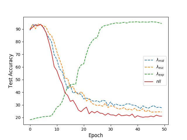
showing that encourages learning more than while provides stronger robustness. It is possible that might slows down training, and if better training speed is desired, we expect using is better. See Figure 6; we show the training trajectory of three different schemes vs. that of loss. We see that, as expected, all three schemes results in better performance than at convergence. The scheme offers stronger robustness while reducing the training speed, while the other two schemes learns faster. While our experiments focuses on showing the effectiveness of , we encourage the practitioners to also try out when necessary. We also expected to be helpful for standard image classification tasks when the noise rate is small but unknown.
Appendix F Assymetric Noise Experiment
The assymetric noise we experiment with is called the pairflip type of noise, which is defined in (Yu et al. 2019). See Table 4. Throughout our experiments, we used a uniform learning rate with batch sizes of . Our MNIST and CIFAR10 models were trained with Adam optimizers, while IMDB was trained with an experimental optimizer. For MNIST and CIFAR10, we used a 2-layer CNN, MNIST with 2 fully connected layers and CIFAR10 with 3. Accuracy was recorded after a previously set number of epochs (except under the early stopping criterion experiments). In IMDB, we used a single-layer LSTM. In MNIST, the model was trained for epochs, using auto-scheduled gambler’s loss throughout. In CIFAR10 and IMDB, the model was trained for epochs, with the first epochs run with regular cross-entropy loss. We note that the proposed method also achieves the SOTA results on assymetric noise.
| Dataset | nll loss | Coteaching+ | Loss | Gamblers | Gamblers + schedule |
| MNIST | |||||
| MNIST | |||||
| MNIST | |||||
| CIFAR10 | |||||
| CIFAR10 | |||||
| CIFAR10 |
Appendix G Concerning Learnability
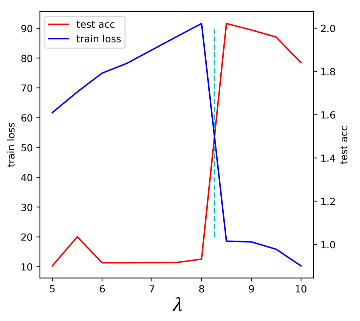
It is noticed in Section 4.2 that the role of is two-fold. On the one hand, it controls the robustness of the model to mislabeling in the dataset. On the other hand, it controls the learnability of the training set. In fact, experiments reveal that the phenomenon is quite dramatic, in the sense that a phase transition-like behavior exists when different is used.
In particular, we note that there is a “good” range for hyperparameter and a bad range. The good range is between a critical value and (non-inclusive) and the bad range is smaller than . See Figure 7 for an example on MNIST with . We see that, in the good range, reducing improves robustness, resultin in performance improvement by more than accuracy; however, reducing below makes learning impossible. In this example, we experimentally pin-down to lie in .