Distributed Averaging Methods for Randomized Second Order Optimization

In this work, we study averaging for randomized second order methods for Least Squares problems, as well as a more general class of convex optimization problems.

Random projections are a popular way of performing randomized dimensionality reduction, which are widely used in many computational and learning problems  (Vempala 2005; Mahoney 2011; Woodruff 2014; Drineas & Mahoney 2016). Many works have studied randomized sketching methods for least squares and optimization problems (Avron et al. 2010; Rokhlin et al. 2009; Drineas et al. 2011; Pilanci & Wainwright 2015; Pilanci & Wainwright 2017; Wang et al. 2017; Wang et al. 2018b).

Our results on least squares regression improve on the results in (Wang et al. 2017) for averaging multiple sketched solutions. In particular, in (Wang et al. 2017), the sketched sub-problems use the same regularization parameter as the original problem, which leads to biased solutions. We analyze the bias of the averaged solution, and provide explicit formulas for selecting the regularization parameter of the sketched sub-problems to achieve unbiasedness. In addition, we analyze the convergence rate of the distributed version of the iterative Hessian sketch algorithm which was introduced in (Pilanci & Wainwright 2016).

One of the main contributions of this work is developing bias correction for averaging sketched solutions. Namely, the setting considered in (Wang et al. 2018b) is based on a distributed second order optimization method that involves averaging approximate update directions. However, in that work, the bias was not taken into account which degrades accuracy and limits applicability to massively parallel computation. We additionally provide results for the unregularized case, which corresponds to the distributed version of the Newton sketch algorithm introduced in (Pilanci & Wainwright 2017)

In Section 2, we describe the problem setup and notation and discuss different types of sketching matrices we consider. Section 3 presents Theorem 1 and Corollary 1 which establish the error decay and convergence properties of the distributed iterative Hessian sketch algorithm given in Algorithm 1. Section 4 presents Theorem 2, which characterizes bias conditions for the averaged ridge regression estimator. Sections 5 and 6 provide an analysis of the bias of estimators for the averaged Newton sketch update directions with no regularization (Theorem 3) and regularization (Theorem 4), respectively. Section 7 discusses two optimization problems where our results can be applied. In Section 8, we present our numerical results.

The proofs of the theorems and lemmas are provided in the supplementary material.

We consider a distributed computing model where we have $q$ worker nodes and a single central node, i.e., master node. The workers may only be allowed to communicate with the master node. The master collects the outputs of the worker nodes and returns the averaged result. For iterative algorithms, this step serves as a synchronization point.

Throughout the text, we provide exact formulas for the bias and variance of sketched solutions. All the expectations in the paper are with respect to the randomness over the sketching matrices, where no randomness assumptions are made for the data.

Throughout the text, we use hats (e.g. $\hat{x}_{k}$) to denote the estimator for the $k$’th sketch and bars (e.g. $\bar{x}$) to denote the averaged estimator. We use $f(.)$ to denote the objective of whichever optimization problem is being considered at that point in the text.

We use $S\in\mathbb{R}^{m\times n}$ to denote random sketching matrices. For non-iterative distributed algorithms, we use $S_{k}\in\mathbb{R}^{m\times n}$ to refer to the sketching matrix used by worker $k$. For iterative algorithms, $S_{t,k}\in\mathbb{R}^{m\times n}$ is used to denote the sketching matrix used by worker $k$ in iteration $t$. We assume the sketching matrices are appropriately scaled to satisfy $\mathbb{E}[S_{t,k}^{T}S_{t,k}]=I_{n}$ and are independently drawn by each worker. We omit the subscripts in $S_{k}$ and $S_{t,k}$ for simplicity whenever it does not cause confusion.

For problems involving regularization, we use $\lambda_{1}$ for the regularization coefficient of the original problem, and $\lambda_{2}$ for the regularization coefficient of the sketched sub-problems.

We consider various sketching matrices in this work including Gaussian sketch, uniform sampling, randomized Hadamard based sketch, Sparse Johnson-Lindenstrauss Transform (SJLT), and hybrid sketch. We now briefly describe each of these sketching methods:

1. 1.

   Gaussian sketch: Entries of $S\in\mathbb{R}^{m\times n}$ are i.i.d. and sampled from the Gaussian distribution. Sketching a matrix $A\in\mathbb{R}^{n\times d}$ using Gaussian sketch requires matrix multiplication $SA$ which has computational complexity equal to $\mathcal{O}(mnd)$.

2. 2.

   Randomized Hadamard based sketch: The sketch matrix in this case can be represented as $S=PHD$ where $P\in\mathbb{R}^{m\times n}$ is for uniform sampling of $m$ rows out of $n$ rows, $H\in\mathbb{R}^{n\times n}$ is the Hadamard matrix, and $D\in\mathbb{R}^{n\times n}$ is a diagonal matrix with diagonal entries sampled randomly from the Rademacher distribution. Multiplication by $D$ to obtain $DA$ requires $\mathcal{O}(nd)$ scalar multiplications. Hadamard transform can be implemented as a fast transform with complexity $\mathcal{O}(n\log(n))$ per column, and a total complexity of $\mathcal{O}(nd\log(n))$ to sketch all $d$ columns of $DA$. We note that because $P$ reduces the row dimension down to $m$, it might be possible to devise a more efficient way to perform sketching with lower computational complexity.

3. 3.

   Uniform sampling: Uniform sampling randomly selects $m$ rows out of the $n$ rows of $A$ where the probability of any row being selected is the same.

4. 4.

   Sparse Johnson-Lindenstrauss Transform (SJLT) (Nelson & Nguyên 2013): The sketching matrix for SJLT is a sparse matrix where each column has exactly $s$ nonzero entries and the columns are independently distributed. The nonzero entries are sampled from the Rademacher distribution. It takes $\mathcal{O}(snd/m)$ addition operations to sketch a data matrix using SJLT.

5. 5.

   Hybrid sketch: The method that we refer to as hybrid sketch is a sequential application of two different sketching methods. In particular, it might be computationally feasible for worker nodes to sample as much data as possible ($m_{2}$ rows) and then reduce the dimension of the available data to the final sketch dimension $m$ using another sketch with better properties than uniform sampling such as Gaussian sketch or SJLT. For instance, hybrid sketch with uniform sampling followed by Gaussian sketch has computational complexity $\mathcal{O}(mm_{2}d)$.

Let us now consider the scenario where we have different sketch sizes in each worker. This situation frequently arises in heterogeneous computing environments. Specifically, let us assume that the sketch size for worker $k$ is $m_{k}$, $k=1,2,...,q$. By Theorem 2, by choosing the regularization parameter for worker $k$ as

it is possible to obtain unbiased estimators $\hat{x}_{k}$ for $k=1,...,q$ and hence an unbiased averaged result $\bar{x}$. Note that here we assume that the sketch size for each worker satisfies the condition in Theorem 2 for zero bias in each estimator $\hat{x}_{k}$, that is, either $m_{k}>d$ or $m_{k}\leq d$ and $\lambda_{1}\geq\sigma^{2}(d/m_{k}-1)$.

We analyze the bias and the variance of the update directions for distributed Newton sketch, and give exact expressions for Gaussian sketching matrices.

Let $\Delta_{t}^{*}$ denote the exact Newton update direction at iteration $t$, then

and let $\hat{\Delta}_{k,t}$ denote the approximate update direction outputted by worker $k$ at iteration $t$, which is given by

Note that the step size for the averaged update direction will be calculated as $\alpha_{2}=\alpha_{1}\alpha_{s}$. Theorem 3 characterizes how the update directions needs to be modified to obtain an unbiased update direction, and a minimum variance estimator for the update direction.

Figure 2 demonstrates that choosing $\alpha_{2}=\alpha_{1}\alpha_{s}$ where $\alpha_{s}$ is calculated using the unbiased estimator formula leads to faster decrease of the objective value when the number of workers is large. If the number of workers is small, one should choose the step size that minimizes variance instead. Figure 2(a) illustrates that the blue curve with squares is in fact the best one could hope to achieve as it is very close to the best cyan dotted line.

Non-identical sketch sizes: Theorem 3 establishes that whenever the sketch dimension varies among workers, it is possible to obtain an unbiased update direction by computing $\alpha_{s}$ for every worker individually.

Let us consider the logistic regression problem with $\ell_{2}$ penalty given by $\textrm{minimize}_{x}f(x)$ where

and $p\in\mathbb{R}^{n}$ is defined such that $p_{i}=1/(1+\exp(-\tilde{a}_{i}^{T}x))$. $\tilde{a}_{i}$ represents the $i$’th row of the data matrix $A\in\mathbb{R}^{n\times d}$. The output vector is denoted by $y\in\mathbb{R}^{n}$.

The gradient and Hessian for $f(x)$ are as follows

$D$ is a diagonal matrix with the entries of the vector $p(1-p)$ as its diagonal entries. The sketched Hessian matrix in this case can be formed as $(SD^{1/2}A)^{T}(SD^{1/2}A)+\lambda_{2}^{*}I_{d}$ and $\lambda_{2}^{*}$ can be calculated using (13), setting $\sigma$ the mean of singular values of $D^{1/2}A$ in the formula. Because $D$ changes every iteration, it might be computationally infeasible to re-compute the mean of the singular values. However, we have found through experiments that it is not required to compute the exact value of the mean of the singular values. For instance, setting $\sigma$ to the mean of the diagonals of $D^{1/2}$ as a heuristic works sufficiently well.

Next, we consider the following inequality constrained optimization problem,

where $A\in\mathbb{R}^{n\times d}$, and $c\in\mathbb{R}^{d}$ are the problem data, and $\lambda\in\mathbb{R}$ is a positive scalar. Note that this problem is the dual of the Lasso problem given by $\text{min}_{x}$ $\lambda\|x\|_{1}+\frac{1}{2}\|Ax-c\|_{2}^{2}$.

The above problem can be tackled by the standard log-barrier method (Boyd & Vandenberghe 2004), by solving sequences of unconstrained barrier penalized problems as follows

where $\tilde{a}_{i}$ represents the $i$’th row of $A$. The gradient and Hessian of the objective are given by

Here $A_{c}=[A^{T},-A^{T}]^{T}$ and $D$ is a diagonal matrix with the element-wise inverse the vector $(A_{c}x-\mathbf{1}_{2n\times 1})$ as its diagonal entries. $\mathbf{1}_{2n\times 1}$ is a length-$2n$ vector of all $1$’s. The sketched Hessian can be written in the form of $(SDA_{c})^{T}(SDA_{c})+\lambda_{2}I_{d}$.

Remark: Since we have the term $2\lambda_{1}I_{d}$ in $H$ (instead of $\lambda_{1}I_{d}$), we need to plug in $2\lambda_{1}$ instead of $\lambda_{1}$ in the formula for computing $\lambda_{2}^{*}$.

We have evaluated the distributed IHS algorithm on the serverless computing platform AWS Lambda. In the implementation, each serverless function is responsible for solving one sketched problem per iteration. Workers wait once they finish their computation for that iteration until the next iterate $x_{t+1}$ becomes available. The master node, which is another AWS Lambda worker, is responsible for collecting and averaging the worker outputs and broadcasting the next iterate $x_{t+1}$.

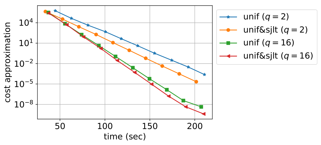
Figure 3 shows the scaled difference between the cost for the $t$’th iterate and the optimal cost (i.e. $(f(x_{t})-f(x^{*}))/f(x^{*})$) versus iteration number $t$ for the distributed IHS algorithm given in Algorithm 1. Due to the relatively small size of the problem, we have each worker compute the exact gradient without requiring an additional communication round per iteration to form the full gradient. We note that, in problems where it’s not feasible for workers to form the full gradient due to limited memory, one can include an additional communication round where each worker sends their local gradient to the master node, and the master node forms the full gradient and distributes it to the worker nodes.

Figure 4 compares various sketches with and without bias correction for the distributed Newton sketch algorithm when it is used to solve the problem given in (7.2). For each sketch, we have plotted the performance for $\lambda_{2}=\lambda_{1}$ and the bias corrected version $\lambda_{2}=\lambda_{2}^{*}$. The bias corrected versions are shown as the dotted lines. In these experiments, we have set $\sigma$ to the minimum of the singular values of $DA$ as we have observed that setting $\sigma$ to the minimum of the singular values of $DA$ performed better than setting it to their mean.

Even though we have derived the bias correction formula for Gaussian sketch, we observe that it improves the performance of SJLT as well. We see that Gaussian sketch and SJLT perform the best out of the 4 sketches we have experimented with. We note that computational complexity of sketching for SJLT is lower than it is for Gaussian sketch, and hence the natural choice would be to use SJLT in this case.

Figure 5 shows the cost against time when we solve the problem given in (7.2) for large scale data on AWS Lambda using the distributed Newton sketch algorithm. The setting in this experiment is such that each worker has access to a different subset of data, and there is no additional sketching applied. The dataset used is randomly generated and the goal here is to demonstrate the scalability of the algorithm and the serverless implementation. The size of the data matrix $A$ is $44$ GB.

In the serverless implementation, we reuse the serverless functions during the course of the algorithm, meaning that the same $q=100$ functions are used for every iteration. We note that every iteration requires two rounds of communication with the master node. The first round is for the communication of the local gradients, and the second round is for the approximate update directions. The master node, also a serverless function, is also reused across iterations. Figure 5 illustrates that each iteration takes a different amount of time and iteration times can be as short as $5$ seconds. The reason for some iterations taking much longer times is what is referred to as the straggler problem, which is a phenomenon commonly encountered in distributed computing. More precisely, the iteration time is determined by the slowest of the $q=100$ nodes and nodes often slow down for a variety of reasons causing stragglers. A possible solution to the issue of straggling nodes is to use error correcting codes to insert redundancy to computation and hence to avoid waiting for the outputs of all of the worker nodes (Lee et al. 2018). We identify that implementing straggler mitigation for solving large scale problems via approximate second order optimization methods such as distributed Newton sketch is a promising direction.

References

• Avron et al. (2010) Avron, H., Maymounkov, P., and Toledo, S. Blendenpik: Supercharging lapack’s least-squares solver. SIAM Journal on Scientific Computing, 32(3):1217–1236, 2010.
• Boyd & Vandenberghe (2004) Boyd, S. and Vandenberghe, L. Convex optimization. Cambridge university press, 2004.
• Drineas & Mahoney (2016) Drineas, P. and Mahoney, M. W. RandNLA: randomized numerical linear algebra. Communications of the ACM, 59(6):80–90, 2016.
• Drineas et al. (2011) Drineas, P., Mahoney, M. W., Muthukrishnan, S., and Sarlós, T. Faster least squares approximation. Numerische mathematik, 117(2):219–249, 2011.
• Lacotte & Pilanci (2019) Lacotte, J. and Pilanci, M. Faster least squares optimization, 2019.
• Lee et al. (2018) Lee, K., Lam, M., Pedarsani, R., Papailiopoulos, D., and Ramchandran, K. Speeding up distributed machine learning using codes. IEEE Transactions on Information Theory, 64(3):1514–1529, March 2018.
• Liu & Dobriban (2019) Liu, S. and Dobriban, E. Ridge regression: Structure, cross-validation, and sketching, 2019.
• Mahoney (2011) Mahoney, M. W. Randomized algorithms for matrices and data. Foundations and Trends® in Machine Learning, 3(2):123–224, 2011.
• Nelson & Nguyên (2013) Nelson, J. and Nguyên, H. L. Osnap: Faster numerical linear algebra algorithms via sparser subspace embeddings. In Foundations of Computer Science (FOCS), 2013 IEEE 54th Annual Symposium on, pp. 117–126. IEEE, 2013.
• Pilanci & Wainwright (2015) Pilanci, M. and Wainwright, M. J. Randomized sketches of convex programs with sharp guarantees. IEEE Transactions on Information Theory, 61(9):5096–5115, 2015.
• Pilanci & Wainwright (2016) Pilanci, M. and Wainwright, M. J. Iterative hessian sketch: Fast and accurate solution approximation for constrained least-squares. The Journal of Machine Learning Research, 17(1):1842–1879, 2016.
• Pilanci & Wainwright (2017) Pilanci, M. and Wainwright, M. J. Newton sketch: A near linear-time optimization algorithm with linear-quadratic convergence. SIAM Journal on Optimization, 27(1):205–245, 2017.
• Reisizadeh et al. (2017) Reisizadeh, A., Prakash, S., Pedarsani, R., and Avestimehr, S. Coded computation over heterogeneous clusters. In 2017 IEEE International Symposium on Information Theory (ISIT), pp. 2408–2412, June 2017. doi: 10.1109/ISIT.2017.8006961.
• Rokhlin et al. (2009) Rokhlin, V., Szlam, A., and Tygert, M. A randomized algorithm for principal component analysis. SIAM Journal on Matrix Analysis and Applications, 31(3):1100–1124, 2009.
• Vempala (2005) Vempala, S. S. The random projection method, volume 65. American Mathematical Soc., 2005.
• Wang et al. (2018a) Wang, C.-C., Tan, K. L., Chen, C.-T., Lin, Y.-H., Keerthi, S. S., Mahajan, D., Sundararajan, S., and Lin, C.-J. Distributed newton methods for deep neural networks. Neural computation, (Early Access):1–52, 2018a.
• Wang et al. (2017) Wang, S., Gittens, A., and Mahoney, M. W. Sketched ridge regression: Optimization perspective, statistical perspective, and model averaging. J. Mach. Learn. Res., 18(1):8039–8088, January 2017.
• Wang et al. (2018b) Wang, S., Roosta, F., Xu, P., and Mahoney, M. W. Giant: Globally improved approximate newton method for distributed optimization. In Advances in Neural Information Processing Systems 31, pp. 2332–2342. Curran Associates, Inc., 2018b.
• Woodruff (2014) Woodruff, D. P. Sketching as a tool for numerical linear algebra. Foundations and Trends® in Theoretical Computer Science, 10(1–2):1–157, 2014.
10 Supplementary File
We give the proofs for the all the lemmas and theorems in the supplementary file.
Note: A Jupyter notebook (.ipynb) containing code has been separately uploaded (also as a .py file). The code requires Python 3 to run.
10.1 Proofs of Theorems in Section 3
Proof of Theorem 1..
The update rule for distributed IHS is given as
xt+1=xt−μ​1q​∑k=1q(AT​St,kT​St,k​A)−1​AT​(A​xt−b).\displaystyle x_{t+1}=x_{t}-\mu\frac{1}{q}\sum_{k=1}^{q}(A^{T}S_{t,k}^{T}S_{t,k}A)^{-1}A^{T}(Ax_{t}-b). (17)
Let us decompose bb as b=A​x∗+b⟂b=Ax^{*}+b^{\perp} and note that AT​b⟂=0A^{T}b^{\perp}=0 which gives us:
xt+1=xt−μ​1q​∑k=1q(AT​St,kT​St,k​A)−1​AT​A​et.\displaystyle x_{t+1}=x_{t}-\mu\frac{1}{q}\sum_{k=1}^{q}(A^{T}S_{t,k}^{T}S_{t,k}A)^{-1}A^{T}Ae_{t}. (18)
Subtracting x∗x^{*} from both sides, we obtain an equation in terms of the error vector ete_{t} only:
et+1\displaystyle e_{t+1} =et−μ​1q​∑k=1q(AT​St,kT​St,k​A)−1​AT​A​et\displaystyle=e_{t}-\mu\frac{1}{q}\sum_{k=1}^{q}(A^{T}S_{t,k}^{T}S_{t,k}A)^{-1}A^{T}Ae_{t}
=(I−μ​1q​∑k=1q(AT​St,kT​St,k​A)−1​AT​A)​et.\displaystyle=\left(I-\mu\frac{1}{q}\sum_{k=1}^{q}(A^{T}S_{t,k}^{T}S_{t,k}A)^{-1}A^{T}A\right)e_{t}.
Let us multiply both sides by AA from the left and define Qt,k≔A​(AT​St,kT​St,k​A)−1​ATQ_{t,k}\coloneqq A(A^{T}S_{t,k}^{T}S_{t,k}A)^{-1}A^{T} and we will have the following equation:
et+1A\displaystyle e^{A}_{t+1} =(I−μ​1q​∑k=1qQt,k)​etA.\displaystyle=\left(I-\mu\frac{1}{q}\sum_{k=1}^{q}Q_{t,k}\right)e^{A}_{t}.
We now analyze the expectation of ℓ2\ell_{2} norm of et+1Ae^{A}_{t+1}:
𝔼⁡[‖et+1A‖22]\displaystyle\mathbb{E}[||e^{A}_{t+1}||_{2}^{2}] =𝔼⁡[‖1q​∑k=1q(I−μ​Qt,k)​etA‖22]\displaystyle=\mathbb{E}\left[\left\|\frac{1}{q}\sum_{k=1}^{q}(I-\mu Q_{t,k})e^{A}_{t}\right\|_{2}^{2}\right]
=1q2​𝔼​[∑k=1q∑l=1q⟨(I−μ​Qt,k)​etA,(I−μ​Qt,l)​etA⟩]\displaystyle=\frac{1}{q^{2}}\mathbb{E}\left[\sum_{k=1}^{q}\sum_{l=1}^{q}\langle(I-\mu Q_{t,k})e^{A}_{t},(I-\mu Q_{t,l})e^{A}_{t}\rangle\right]
=1q2​∑k=1q∑l=1q𝔼⁡[⟨(I−μ​Qt,k)​etA,(I−μ​Qt,l)​etA⟩].\displaystyle=\frac{1}{q^{2}}\sum_{k=1}^{q}\sum_{l=1}^{q}\mathbb{E}\left[\langle(I-\mu Q_{t,k})e^{A}_{t},(I-\mu Q_{t,l})e^{A}_{t}\rangle\right]. (19)
The contribution for k≠lk\neq l in the double summation of (10.1) is equal to zero because for k≠lk\neq l, we have
𝔼⁡[⟨(I−μ​Qt,k)​etA,(I−μ​Qt,l)​etA⟩]\displaystyle\mathbb{E}\left[\langle(I-\mu Q_{t,k})e^{A}_{t},(I-\mu Q_{t,l})e^{A}_{t}\rangle\right] =⟨𝔼⁡[(I−μ​Qt,k)​etA],𝔼⁡[(I−μ​Qt,l)​etA]⟩\displaystyle=\langle\mathbb{E}[(I-\mu Q_{t,k})e^{A}_{t}],\mathbb{E}[(I-\mu Q_{t,l})e^{A}_{t}]\rangle
=⟨𝔼⁡[(I−μ​Qt,k)​etA],𝔼⁡[(I−μ​Qt,k)​etA]⟩\displaystyle=\langle\mathbb{E}[(I-\mu Q_{t,k})e^{A}_{t}],\mathbb{E}[(I-\mu Q_{t,k})e^{A}_{t}]\rangle
=‖𝔼⁡[(I−μ​Qt,k)​etA]‖22.\displaystyle=\left\|\mathbb{E}[(I-\mu Q_{t,k})e^{A}_{t}]\right\|_{2}^{2}.
The term in the last line above is zero for μ=1θ1\mu=\frac{1}{\theta_{1}}:
𝔼⁡[(I−μ​Qt,k)​etA]\displaystyle\mathbb{E}[(I-\mu Q_{t,k})e^{A}_{t}] =𝔼⁡[(I−μ​A​(AT​St,kT​St,k​A)−1​AT)​etA]\displaystyle=\mathbb{E}[(I-\mu A(A^{T}S_{t,k}^{T}S_{t,k}A)^{-1}A^{T})e^{A}_{t}]
=(I−μ​θ1​A​(AT​A)−1​AT)​etA\displaystyle=(I-\mu\theta_{1}A(A^{T}A)^{-1}A^{T})e^{A}_{t}
=(I−μ​θ1​U​UT)​etA\displaystyle=(I-\mu\theta_{1}UU^{T})e^{A}_{t}
=(I−U​UT)​etA\displaystyle=(I-UU^{T})e^{A}_{t}
=0\displaystyle=0
where we used A=U​Σ​VTA=U\Sigma V^{T}. For the rest of the proof, we assume that we set μ=1/θ1\mu=1/\theta_{1}. Now that we know the contribution from terms with k≠lk\neq l is zero, the expansion in (10.1) can be rewritten:
𝔼⁡[‖et+1A‖22]\displaystyle\mathbb{E}[||e^{A}_{t+1}||_{2}^{2}] =1q2​∑k=1q𝔼⁡[⟨(I−μ​Qt,k)​etA,(I−μ​Qt,k)​etA⟩]\displaystyle=\frac{1}{q^{2}}\sum_{k=1}^{q}\mathbb{E}\left[\langle(I-\mu Q_{t,k})e^{A}_{t},(I-\mu Q_{t,k})e^{A}_{t}\rangle\right]
=1q2​∑k=1q𝔼⁡[‖(I−μ​Qt,k)​etA‖22]\displaystyle=\frac{1}{q^{2}}\sum_{k=1}^{q}\mathbb{E}[||(I-\mu Q_{t,k})e^{A}_{t}||_{2}^{2}]
=1q​𝔼​[‖(I−μ​Qt,1)​etA‖22]\displaystyle=\frac{1}{q}\mathbb{E}[||(I-\mu Q_{t,1})e^{A}_{t}||_{2}^{2}]
=1q​(‖etA‖22+μ2​𝔼​[‖Qt,1​etA‖22]−2​μ​(etA)T​𝔼​[Qt,1]​etA)\displaystyle=\frac{1}{q}\left(||e^{A}_{t}||_{2}^{2}+\mu^{2}\mathbb{E}[||Q_{t,1}e^{A}_{t}||_{2}^{2}]-2\mu(e^{A}_{t})^{T}\mathbb{E}[Q_{t,1}]e^{A}_{t}\right)
=1q​(μ2​𝔼​[‖Qt,1​etA‖22]−‖etA‖22)\displaystyle=\frac{1}{q}\left(\mu^{2}\mathbb{E}[||Q_{t,1}e^{A}_{t}||_{2}^{2}]-||e^{A}_{t}||_{2}^{2}\right)
=1q​(μ2​(etA)T​𝔼​[Qt,1T​Qt,1]​etA−‖etA‖22)\displaystyle=\frac{1}{q}\left(\mu^{2}(e^{A}_{t})^{T}\mathbb{E}[Q_{t,1}^{T}Q_{t,1}]e^{A}_{t}-||e^{A}_{t}||_{2}^{2}\right)
The term 𝔼⁡[Qt,1T​Qt,1]\mathbb{E}[Q_{t,1}^{T}Q_{t,1}] can be simplified using SVD decomposition A=U​Σ​VTA=U\Sigma V^{T}. This gives us Qt,k=U​(UT​St,kT​St,k​U)−1​UTQ_{t,k}=U(U^{T}S_{t,k}^{T}S_{t,k}U)^{-1}U^{T} and furthermore we have:
𝔼⁡[Qt,1T​Qt,1]\displaystyle\mathbb{E}[Q_{t,1}^{T}Q_{t,1}] =𝔼⁡[U​(UT​St,1T​St,1​U)−1​UT​U​(UT​St,1T​St,1​U)−1​UT]\displaystyle=\mathbb{E}[U(U^{T}S_{t,1}^{T}S_{t,1}U)^{-1}U^{T}U(U^{T}S_{t,1}^{T}S_{t,1}U)^{-1}U^{T}]
=𝔼⁡[U​(UT​St,1T​St,1​U)−1​(UT​St,1T​St,1​U)−1​UT]\displaystyle=\mathbb{E}[U(U^{T}S_{t,1}^{T}S_{t,1}U)^{-1}(U^{T}S_{t,1}^{T}S_{t,1}U)^{-1}U^{T}]
=U​𝔼​[(UT​St,1T​St,1​U)−2]​UT\displaystyle=U\mathbb{E}[(U^{T}S_{t,1}^{T}S_{t,1}U)^{-2}]U^{T}
=θ2​U​UT.\displaystyle=\theta_{2}UU^{T}.
Plugging this in, we obtain:
𝔼⁡[‖et+1A‖22]\displaystyle\mathbb{E}[||e^{A}_{t+1}||_{2}^{2}] =1q​(θ2​μ2​(etA)T​U​UT​etA−‖etA‖22)\displaystyle=\frac{1}{q}\left(\theta_{2}\mu^{2}(e^{A}_{t})^{T}UU^{T}e^{A}_{t}-||e^{A}_{t}||_{2}^{2}\right)
=1q​(θ2​μ2​‖UT​etA‖22−‖etA‖22)\displaystyle=\frac{1}{q}\left(\theta_{2}\mu^{2}||U^{T}e^{A}_{t}||_{2}^{2}-||e^{A}_{t}||_{2}^{2}\right)
=1q​(θ2​μ2​‖etA‖22−‖etA‖22)\displaystyle=\frac{1}{q}\left(\theta_{2}\mu^{2}||e^{A}_{t}||_{2}^{2}-||e^{A}_{t}||_{2}^{2}\right)
=θ2​μ2−1q​‖etA‖22\displaystyle=\frac{\theta_{2}\mu^{2}-1}{q}||e^{A}_{t}||_{2}^{2}
=1q​(θ2θ12−1)​‖etA‖22\displaystyle=\frac{1}{q}\left(\frac{\theta_{2}}{\theta_{1}^{2}}-1\right)||e^{A}_{t}||_{2}^{2}
∎
Proof of Corollary 1..
Taking the expectation with respect to St,kS_{t,k}, k=1,…,qk=1,...,q of both sides of the equation given in Theorem 1, we obtain
𝔼⁡[‖et+1A‖22]=1q​(θ2θ12−1)​𝔼​[‖etA‖22].\displaystyle\mathbb{E}[||e^{A}_{t+1}||_{2}^{2}]=\frac{1}{q}\left(\frac{\theta_{2}}{\theta_{1}^{2}}-1\right)\mathbb{E}[||e^{A}_{t}||_{2}^{2}]\,.
This gives us the relationship between the initial error (when we initialize x0x_{0} to be the zero vector) and the expected error in iteration tt:
𝔼⁡[‖etA‖22]=1qt​(θ2θ12−1)t​‖A​x∗‖22.\displaystyle\mathbb{E}[||e^{A}_{t}||_{2}^{2}]=\frac{1}{q^{t}}\left(\frac{\theta_{2}}{\theta_{1}^{2}}-1\right)^{t}||Ax^{*}||_{2}^{2}.
It follows that the expected error reaches ϵ\epsilon-accuracy with respect to the initial error at iteration TT where:
1qT​(θ2θ12−1)T\displaystyle\frac{1}{q^{T}}\left(\frac{\theta_{2}}{\theta_{1}^{2}}-1\right)^{T} =ϵ\displaystyle=\epsilon
qT​(θ2θ12−1)−T\displaystyle q^{T}\left(\frac{\theta_{2}}{\theta_{1}^{2}}-1\right)^{-T} =1ϵ\displaystyle=\frac{1}{\epsilon}
T⁡(log⁡(q)−log⁡(θ2θ12−1))\displaystyle T\left(\log(q)-\log\left(\frac{\theta_{2}}{\theta_{1}^{2}}-1\right)\right) =log⁡(1/ϵ)\displaystyle=\log(1/\epsilon)
T\displaystyle T =log⁡(1/ϵ)log⁡(q)−log⁡(θ2θ12−1).\displaystyle=\frac{\log(1/\epsilon)}{\log(q)-\log\left(\frac{\theta_{2}}{\theta_{1}^{2}}-1\right)}.
Each iteration requires communicating a dd-dimensional vector for every worker, and we have qq workers and the algorithm runs for TT iterations, hence the communication load is T​q​dTqd.
The computational load per worker at each iteration involves the following numbers of operations:
• •
Sketching AA: m​n​dmnd multiplications
Computing H~t,k\tilde{H}_{t,k}: m​d2md^{2} multiplications
Computing gtg_{t}: 𝒪⁡(n​d)\mathcal{O}(nd) operations
Solving H~t,k−1​gt\tilde{H}_{t,k}^{-1}g_{t}: 𝒪⁡(d3)\mathcal{O}(d^{3}) operations.
10.2 Proofs of Theorems in Section 4
Proof of Lemma 2..
In the following, we assume that we are in the regime where nn approaches infinity.
The expectation term 𝔼⁡[(UT​ST​S​U+λ2​I)−1]\mathbb{E}[(U^{T}S^{T}SU+\lambda_{2}I)^{-1}] is equal to the identity matrix times a scalar (i.e. c​IdcI_{d}) because it is signed permutation invariant, which we show as follows. Let P∈ℝd×dP\in\mathbb{R}^{d\times d} be a permutation matrix and D∈ℝd×dD\in\mathbb{R}^{d\times d} be an invertible diagonal sign matrix (−1-1 and +1+1’s on the diagonals). A matrix MM is signed permutation invariant if (D​P)​M​(D​P)T=M(DP)M(DP)^{T}=M. We note that the signed permutation matrix is orthogonal: (D​P)T​(D​P)=PT​DT​D​P=PT​P=Id(DP)^{T}(DP)=P^{T}D^{T}DP=P^{T}P=I_{d}, which we later use.
(D​P)​𝔼S​[(UT​ST​S​U+λ2​I)−1]​(D​P)T\displaystyle(DP)\mathbb{E}_{S}[(U^{T}S^{T}SU+\lambda_{2}I)^{-1}](DP)^{T} =𝔼S​[(D​P)​(UT​ST​S​U+λ2​I)−1​(D​P)T]\displaystyle=\mathbb{E}_{S}[(DP)(U^{T}S^{T}SU+\lambda_{2}I)^{-1}(DP)^{T}]
=𝔼S​[((D​P)T​UT​ST​S​U​(D​P)+λ2​I)−1]\displaystyle=\mathbb{E}_{S}[((DP)^{T}U^{T}S^{T}SU(DP)+\lambda_{2}I)^{-1}]
=𝔼S​U​P​D​[𝔼S​[((D​P)T​UT​ST​S​U​(D​P)+λ2​I)−1|S​U​P​D]]\displaystyle=\mathbb{E}_{SUPD}[\mathbb{E}_{S}[((DP)^{T}U^{T}S^{T}SU(DP)+\lambda_{2}I)^{-1}|SUPD]]
=𝔼S​U​P​D​[((D​P)T​UT​ST​S​U​(D​P)+λ2​I)−1]\displaystyle=\mathbb{E}_{SUPD}[((DP)^{T}U^{T}S^{T}SU(DP)+\lambda_{2}I)^{-1}]
=𝔼S​U′​[(U′T​ST​S​U′+λ2​I)−1]\displaystyle=\mathbb{E}_{SU^{\prime}}[({U^{\prime}}^{T}S^{T}SU^{\prime}+\lambda_{2}I)^{-1}]
where we made the variable change U′=U​D​PU^{\prime}=UDP and note that U′U^{\prime} has orthonormal columns because D​PDP is an orthogonal transformation. S​U​P​DSUPD and S​USU have the same distribution because P​DPD is an orthogonal transformation and SS is a Gaussian matrix. This shows that 𝔼⁡[(UT​ST​S​U+λ2​I)−1]\mathbb{E}[(U^{T}S^{T}SU+\lambda_{2}I)^{-1}] is signed permutation invariant.
Now that we established that 𝔼⁡[(UT​ST​S​U+λ2​I)−1]\mathbb{E}[(U^{T}S^{T}SU+\lambda_{2}I)^{-1}] is equal to the identity matrix times a scalar, we move on to find the value of the scalar. We use the identity 𝔼D​P​[(D​P)​Q​(D​P)T]=tr⁡Qd​Id\mathbb{E}_{DP}[(DP)Q(DP)^{T}]=\frac{\tr Q}{d}I_{d} for Q∈ℝd×dQ\in\mathbb{R}^{d\times d} where the diagonal entries of DD are sampled from the Rademacher distribution and PP is sampled uniformly from the set of all possible permutation matrices. We already established that 𝔼⁡[(UT​ST​S​U+λ2​I)−1]\mathbb{E}[(U^{T}S^{T}SU+\lambda_{2}I)^{-1}] is equal to (D​P)​𝔼S​[(UT​ST​S​U+λ2​I)−1]​(D​P)T(DP)\mathbb{E}_{S}[(U^{T}S^{T}SU+\lambda_{2}I)^{-1}](DP)^{T} for any signed permutation matrix of the form D​PDP. It follows that
𝔼⁡[(UT​ST​S​U+λ2​I)−1]\displaystyle\mathbb{E}[(U^{T}S^{T}SU+\lambda_{2}I)^{-1}] =(D​P)​𝔼S​[(UT​ST​S​U+λ2​I)−1]​(D​P)T\displaystyle=(DP)\mathbb{E}_{S}[(U^{T}S^{T}SU+\lambda_{2}I)^{-1}](DP)^{T}
=1|R|​∑D​P∈R(D​P)​𝔼S​[(UT​ST​S​U+λ2​I)−1]​(D​P)T\displaystyle=\frac{1}{|R|}\sum_{DP\in R}(DP)\mathbb{E}_{S}[(U^{T}S^{T}SU+\lambda_{2}I)^{-1}](DP)^{T}
=𝔼D​P​[(D​P)​𝔼S​[(UT​ST​S​U+λ2​I)−1]​(D​P)T]\displaystyle=\mathbb{E}_{DP}[(DP)\mathbb{E}_{S}[(U^{T}S^{T}SU+\lambda_{2}I)^{-1}](DP)^{T}]
=1d​tr⁡(𝔼S​[(UT​ST​S​U+λ2​I)−1])​Id\displaystyle=\frac{1}{d}\tr(\mathbb{E}_{S}[(U^{T}S^{T}SU+\lambda_{2}I)^{-1}])I_{d}
where we define RR to be the set of all possible signed permutation matrices D​PDP in going from line 1 to line 2.
By Lemma 1, the trace term is equal to d×θ3​(d/m,λ2)d\times\theta_{3}(d/m,\lambda_{2}), which concludes the proof. ∎
Proof of Theorem 2..
Closed form expressions for the optimal solution and the output of the kk’th worker are as follows:
x∗\displaystyle x^{*} =(AT​A+λ1​Id)−1​AT​b,\displaystyle=(A^{T}A+\lambda_{1}I_{d})^{-1}A^{T}b,
x^k\displaystyle\hat{x}_{k} =(AT​SkT​Sk​A+λ2​Id)−1​AT​SkT​Sk​b.\displaystyle=(A^{T}S_{k}^{T}S_{k}A+\lambda_{2}I_{d})^{-1}A^{T}S_{k}^{T}S_{k}b.
Equivalently, x∗x^{*} can be written as:
x∗=arg⁡min⁡‖[Aλ1​Id]​x−[b0d]‖22.\displaystyle x^{*}=\arg\min\left\|\begin{bmatrix}A\\ \sqrt{\lambda_{1}}I_{d}\end{bmatrix}x-\begin{bmatrix}b\\ 0_{d}\end{bmatrix}\right\|_{2}^{2}.
This allows us to decompose [b0d]\begin{bmatrix}b\\ 0_{d}\end{bmatrix} as
[b0d]=[Aλ1​Id]​x∗+b⟂\displaystyle\begin{bmatrix}b\\ 0_{d}\end{bmatrix}=\begin{bmatrix}A\\ \sqrt{\lambda_{1}}I_{d}\end{bmatrix}x^{*}+b^{\perp}
where b⟂=[b1⟂b2⟂]b^{\perp}=\begin{bmatrix}b_{1}^{\perp}\\ b_{2}^{\perp}\end{bmatrix} with b1⟂∈ℝnb_{1}^{\perp}\in\mathbb{R}^{n} and b2⟂∈ℝdb_{2}^{\perp}\in\mathbb{R}^{d}. From the above equation we obtain b2⟂=−λ1​x∗b^{\perp}_{2}=-\sqrt{\lambda_{1}}x^{*} and [ATλ1​Id]​b⟂=AT​b1⟂+λ1​b2⟂=0\begin{bmatrix}A^{T}&\sqrt{\lambda_{1}}I_{d}\end{bmatrix}b^{\perp}=A^{T}b_{1}^{\perp}+\sqrt{\lambda_{1}}b_{2}^{\perp}=0.
The bias of x^k\hat{x}_{k} is given by (omitting the subscript kk in SkS_{k} for simplicity)
𝔼⁡[A⁡(x^k−x∗)]=\displaystyle\mathbb{E}[A(\hat{x}_{k}-x^{*})]=
=𝔼⁡[A​(AT​ST​S​A+λ2​Id)−1​AT​ST​S​b−A​x∗]\displaystyle=\mathbb{E}[A(A^{T}S^{T}SA+\lambda_{2}I_{d})^{-1}A^{T}S^{T}Sb-Ax^{*}]
=𝔼⁡[U​(UT​ST​S​U+λ2​Σ−2)−1​UT​ST​S​b]−A​x∗\displaystyle=\mathbb{E}[U(U^{T}S^{T}SU+\lambda_{2}\Sigma^{-2})^{-1}U^{T}S^{T}Sb]-Ax^{*}
=𝔼⁡[U​(UT​ST​S​U+λ2​Σ−2)−1​UT​ST​S​(A​x∗+b1⟂)]−A​x∗\displaystyle=\mathbb{E}[U(U^{T}S^{T}SU+\lambda_{2}\Sigma^{-2})^{-1}U^{T}S^{T}S(Ax^{*}+b_{1}^{\perp})]-Ax^{*}
=𝔼⁡[U​(UT​ST​S​U+λ2​Σ−2)−1​UT​ST​S​U​Σ​VT​x∗+U​(UT​ST​S​U+λ2​Σ−2)−1​UT​ST​S​b1⟂]−A​x∗\displaystyle=\mathbb{E}[U(U^{T}S^{T}SU+\lambda_{2}\Sigma^{-2})^{-1}U^{T}S^{T}SU\Sigma V^{T}x^{*}+U(U^{T}S^{T}SU+\lambda_{2}\Sigma^{-2})^{-1}U^{T}S^{T}Sb_{1}^{\perp}]-Ax^{*}
=𝔼⁡[U​(UT​ST​S​U+λ2​Σ−2)−1​(UT​ST​S​U+λ2​Σ−2−λ2​Σ−2)​Σ​VT​x∗+U​(UT​ST​S​U+λ2​Σ−2)−1​UT​ST​S​b1⟂]−A​x∗\displaystyle=\mathbb{E}[U(U^{T}S^{T}SU+\lambda_{2}\Sigma^{-2})^{-1}(U^{T}S^{T}SU+\lambda_{2}\Sigma^{-2}-\lambda_{2}\Sigma^{-2})\Sigma V^{T}x^{*}+U(U^{T}S^{T}SU+\lambda_{2}\Sigma^{-2})^{-1}U^{T}S^{T}Sb_{1}^{\perp}]-Ax^{*}
=𝔼⁡[−λ2​U​(UT​ST​S​U+λ2​Σ−2)−1​Σ−1​VT​x∗]+𝔼⁡[U​(UT​ST​S​U+λ2​Σ−2)−1​UT​ST​S​b1⟂].\displaystyle=\mathbb{E}[-\lambda_{2}U(U^{T}S^{T}SU+\lambda_{2}\Sigma^{-2})^{-1}\Sigma^{-1}V^{T}x^{*}]+\mathbb{E}[U(U^{T}S^{T}SU+\lambda_{2}\Sigma^{-2})^{-1}U^{T}S^{T}Sb_{1}^{\perp}].
By the assumption Σ=σ​Id\Sigma=\sigma I_{d}, the bias becomes
𝔼⁡[A⁡(x^k−x∗)]=𝔼⁡[−λ2​σ−1​U​(UT​ST​S​U+λ2​σ−2​Id)−1​VT​x∗]+𝔼⁡[U​(UT​ST​S​U+λ2​σ−2​Id)−1​UT​ST​S​b1⟂].\displaystyle\mathbb{E}[A(\hat{x}_{k}-x^{*})]=\mathbb{E}[-\lambda_{2}\sigma^{-1}U(U^{T}S^{T}SU+\lambda_{2}\sigma^{-2}I_{d})^{-1}V^{T}x^{*}]+\mathbb{E}[U(U^{T}S^{T}SU+\lambda_{2}\sigma^{-2}I_{d})^{-1}U^{T}S^{T}Sb_{1}^{\perp}]. (20)
The first expectation term of (20) can be evaluated using Lemma 2 (as nn goes to infinity):
𝔼⁡[−λ2​σ−1​U​(UT​ST​S​U+λ2​Id)−1​VT​x∗]=−λ2​σ−1​θ3​(d/m,λ2​σ−2)​U​VT​x∗.\displaystyle\mathbb{E}[-\lambda_{2}\sigma^{-1}U(U^{T}S^{T}SU+\lambda_{2}I_{d})^{-1}V^{T}x^{*}]=-\lambda_{2}\sigma^{-1}\theta_{3}(d/m,\lambda_{2}\sigma^{-2})UV^{T}x^{*}. (21)
To find the second expectation term of (20), let us first consider the full SVD of AA given by A=[UU⟂]​[Σ0(n−d)×d]​VTA=\begin{bmatrix}U&U^{\perp}\end{bmatrix}\begin{bmatrix}\Sigma\\ 0_{(n-d)\times d}\end{bmatrix}V^{T} where U∈ℝn×dU\in\mathbb{R}^{n\times d} and U⟂∈ℝn×(n−d)U^{\perp}\in\mathbb{R}^{n\times(n-d)}. The matrix [UU⟂]\begin{bmatrix}U&U^{\perp}\end{bmatrix} is an orthogonal matrix, which implies U​UT+U⟂​(U⟂)T=IdUU^{T}+U^{\perp}(U^{\perp})^{T}=I_{d}. If we insert U​UT+U⟂​(U⟂)T=IdUU^{T}+U^{\perp}(U^{\perp})^{T}=I_{d} between SS and b1⟂b_{1}^{\perp}, the second term of (20) becomes
𝔼⁡[U​(UT​ST​S​U+λ2​σ−2​Id)−1​UT​ST​S​b1⟂]=\displaystyle\mathbb{E}[U(U^{T}S^{T}SU+\lambda_{2}\sigma^{-2}I_{d})^{-1}U^{T}S^{T}Sb_{1}^{\perp}]=
=𝔼⁡[U​(UT​ST​S​U+λ2​σ−2​Id)−1​UT​ST​S​(U​UT+U⟂​(U⟂)T)​b1⟂]\displaystyle=\mathbb{E}[U(U^{T}S^{T}SU+\lambda_{2}\sigma^{-2}I_{d})^{-1}U^{T}S^{T}S(UU^{T}+U^{\perp}(U^{\perp})^{T})b_{1}^{\perp}]
=𝔼⁡[U​(UT​ST​S​U+λ2​σ−2​Id)−1​UT​ST​S​U​UT​b1⟂]+𝔼⁡[U​(UT​ST​S​U+λ2​σ−2​Id)−1​UT​ST​S​U⟂​(U⟂)T​b1⟂]\displaystyle=\mathbb{E}[U(U^{T}S^{T}SU+\lambda_{2}\sigma^{-2}I_{d})^{-1}U^{T}S^{T}SUU^{T}b_{1}^{\perp}]+\mathbb{E}[U(U^{T}S^{T}SU+\lambda_{2}\sigma^{-2}I_{d})^{-1}U^{T}S^{T}SU^{\perp}(U^{\perp})^{T}b_{1}^{\perp}]
=𝔼⁡[U​(UT​ST​S​U+λ2​σ−2​Id)−1​UT​ST​S​U​UT​b1⟂]\displaystyle=\mathbb{E}[U(U^{T}S^{T}SU+\lambda_{2}\sigma^{-2}I_{d})^{-1}U^{T}S^{T}SUU^{T}b_{1}^{\perp}]
=𝔼⁡[U​(UT​ST​S​U+λ2​σ−2​Id)−1​(UT​ST​S​U+λ2​σ−2​Id−λ2​σ−2​Id)​UT​b1⟂]\displaystyle=\mathbb{E}[U(U^{T}S^{T}SU+\lambda_{2}\sigma^{-2}I_{d})^{-1}(U^{T}S^{T}SU+\lambda_{2}\sigma^{-2}I_{d}-\lambda_{2}\sigma^{-2}I_{d})U^{T}b_{1}^{\perp}]
=U⁡(Id−λ2​σ−2​𝔼​[(UT​ST​S​U+λ2​σ−2​Id)−1])​UT​b1⟂\displaystyle=U(I_{d}-\lambda_{2}\sigma^{-2}\mathbb{E}[(U^{T}S^{T}SU+\lambda_{2}\sigma^{-2}I_{d})^{-1}])U^{T}b_{1}^{\perp}
=(1−λ2​σ−2​θ3​(d/m,λ2​σ−2))​U​UT​b1⟂\displaystyle=(1-\lambda_{2}\sigma^{-2}\theta_{3}(d/m,\lambda_{2}\sigma^{-2}))UU^{T}b_{1}^{\perp}
where in the fourth line we have used 𝔼S​[U​(UT​ST​S​U+λ2​σ−2​Id)−1​UT​ST​S​U⟂​(U⟂)T​b1⟂]=𝔼S​U​[𝔼S​[U​(UT​ST​S​U+λ2​σ−2​Id)−1​UT​ST​S​U⟂​(U⟂)T​b1⟂|S​U]]=0\mathbb{E}_{S}[U(U^{T}S^{T}SU+\lambda_{2}\sigma^{-2}I_{d})^{-1}U^{T}S^{T}SU^{\perp}(U^{\perp})^{T}b_{1}^{\perp}]=\mathbb{E}_{SU}[\mathbb{E}_{S}[U(U^{T}S^{T}SU+\lambda_{2}\sigma^{-2}I_{d})^{-1}U^{T}S^{T}SU^{\perp}(U^{\perp})^{T}b_{1}^{\perp}|SU]]=0 since 𝔼S​[S​U⟂|S​U]=0\mathbb{E}_{S}[SU^{\perp}|SU]=0 as UU and U⟂U^{\perp} are orthogonal. The last line follows from Lemma 2, as nn goes to infinity.
Note that UT​b1⟂=λ1​Σ−1​VT​x∗U^{T}b_{1}^{\perp}=\lambda_{1}\Sigma^{-1}V^{T}x^{*} and for Σ=σ​Id\Sigma=\sigma I_{d}, this becomes UT​b1⟂=λ1​σ−1​VT​x∗U^{T}b_{1}^{\perp}=\lambda_{1}\sigma^{-1}V^{T}x^{*}.
Bringing all of these pieces together, we have the bias equal to (as nn goes to infinity):
𝔼⁡[A⁡(x^k−x∗)]\displaystyle\mathbb{E}[A(\hat{x}_{k}-x^{*})] =−λ2​σ−1​θ3​(d/m,λ2​σ−2)​U​VT​x∗+λ1​σ−1​(1−λ2​σ−2​θ3​(d/m,λ2​σ−2))​U​VT​x∗\displaystyle=-\lambda_{2}\sigma^{-1}\theta_{3}(d/m,\lambda_{2}\sigma^{-2})UV^{T}x^{*}+\lambda_{1}\sigma^{-1}(1-\lambda_{2}\sigma^{-2}\theta_{3}(d/m,\lambda_{2}\sigma^{-2}))UV^{T}x^{*}
=σ−1​(λ1−λ2​θ3​(d/m,λ2​σ−2)​(1+λ1​σ−2))​U​VT​x∗.\displaystyle=\sigma^{-1}(\lambda_{1}-\lambda_{2}\theta_{3}(d/m,\lambda_{2}\sigma^{-2})(1+\lambda_{1}\sigma^{-2}))UV^{T}x^{*}.
If there is a value of λ2>0\lambda_{2}>0 that satisfies λ1−λ2​θ3​(d/m,λ2​σ−2)​(1+λ1​σ−2)=0\lambda_{1}-\lambda_{2}\theta_{3}(d/m,\lambda_{2}\sigma^{-2})(1+\lambda_{1}\sigma^{-2})=0, then that value of λ2\lambda_{2} makes x^k\hat{x}_{k} an unbiased estimator. Equivalently,
(−λ2​σ−2+d/m−1+(−λ2​σ−2+d/m−1)2+4​λ2​σ−2​d/m2​σ−2​d/m)\displaystyle\left(\frac{-\lambda_{2}\sigma^{-2}+d/m-1+\sqrt{(-\lambda_{2}\sigma^{-2}+d/m-1)^{2}+4\lambda_{2}\sigma^{-2}d/m}}{2\sigma^{-2}d/m}\right) =λ11+λ1​σ−2\displaystyle=\frac{\lambda_{1}}{1+\lambda_{1}\sigma^{-2}}
−λ2​σ−2+d/m−1+(−λ2​σ−2+d/m−1)2+4​λ2​σ−2​d/m\displaystyle-\lambda_{2}\sigma^{-2}+d/m-1+\sqrt{(-\lambda_{2}\sigma^{-2}+d/m-1)^{2}+4\lambda_{2}\sigma^{-2}d/m} =2​dm​σ2​λ11+λ1​σ−2,\displaystyle=2\frac{d}{m\sigma^{2}}\frac{\lambda_{1}}{1+\lambda_{1}\sigma^{-2}},
where we note that the LHS is a monotonically increasing function of λ2\lambda_{2} in the regime λ2≥0\lambda_{2}\geq 0 and it attains its minimum in this regime at λ2=0\lambda_{2}=0. Analyzing this equation using these observations, for the cases of m>dm>d and m≤dm\leq d separately, we find that for the case of m≤dm\leq d, we need the following to be satisfied for zero bias:
2​dm​σ2​λ11+λ1/σ2\displaystyle 2\frac{d}{m\sigma^{2}}\frac{\lambda_{1}}{1+\lambda_{1}/\sigma^{2}} ≥2​(dm−1),\displaystyle\geq 2\left(\frac{d}{m}-1\right),
λ1\displaystyle\lambda_{1} ≥σ2​(dm−1),\displaystyle\geq\sigma^{2}\left(\frac{d}{m}-1\right),
whereas there is no condition on λ1\lambda_{1} for the case of m>dm>d.
The value of λ2\lambda_{2} that will lead to zero bias is given by
λ2∗=λ1−dm​11+λ1/σ2.\displaystyle\lambda_{2}^{*}=\lambda_{1}-\frac{d}{m}\frac{1}{1+\lambda_{1}/\sigma^{2}}.
10.3 Proofs of Theorems in Section 5
Proof of Theorem 3..
The optimal update direction is given by
Δt∗=((Ht1/2)T​Ht1/2)−1​gt=Ht−1​gt\displaystyle\Delta_{t}^{*}=((H_{t}^{1/2})^{T}H_{t}^{1/2})^{-1}g_{t}=H_{t}^{-1}g_{t}
and the estimate update direction due to a single sketch is given by
Δ^t,k=αs​((Ht1/2)T​St,kT​St,k​Ht1/2)−1​gt.\displaystyle\hat{\Delta}_{t,k}=\alpha_{s}((H_{t}^{1/2})^{T}S_{t,k}^{T}S_{t,k}H_{t}^{1/2})^{-1}g_{t}.
where αs∈ℝ\alpha_{s}\in\mathbb{R} is the step size scaling factor to be determined.
Letting St,kS_{t,k} be a Gaussian sketch, the bias can be written as
𝔼⁡[Ht1/2​(Δ^t,k−Δt∗)]\displaystyle\mathbb{E}[H_{t}^{1/2}(\hat{\Delta}_{t,k}-\Delta_{t}^{*})] =𝔼⁡[αs​Ht1/2​((Ht1/2)T​St,kT​St,k​Ht1/2)−1​gt−Ht1/2​Ht−1​gt]\displaystyle=\mathbb{E}[\alpha_{s}H_{t}^{1/2}((H_{t}^{1/2})^{T}S_{t,k}^{T}S_{t,k}H_{t}^{1/2})^{-1}g_{t}-H_{t}^{1/2}H_{t}^{-1}g_{t}]
=αs​Ht1/2​𝔼​[((Ht1/2)T​St,kT​St,k​Ht1/2)−1]​gt−Ht1/2​Ht−1​gt\displaystyle=\alpha_{s}H_{t}^{1/2}\mathbb{E}[((H_{t}^{1/2})^{T}S_{t,k}^{T}S_{t,k}H_{t}^{1/2})^{-1}]g_{t}-H_{t}^{1/2}H_{t}^{-1}g_{t}
=αs​θ1​Ht1/2​((Ht1/2)T​Ht1/2)−1​gt−Ht1/2​Ht−1​gt\displaystyle=\alpha_{s}\theta_{1}H_{t}^{1/2}((H_{t}^{1/2})^{T}H_{t}^{1/2})^{-1}g_{t}-H_{t}^{1/2}H_{t}^{-1}g_{t}
=(αs​θ1−1)​Ht1/2​Ht−1​gt.\displaystyle=\left(\alpha_{s}\theta_{1}-1\right)H_{t}^{1/2}H_{t}^{-1}g_{t}.
In the third line, we plug in the mean of ((Ht1/2)T​St,kT​St,k​Ht1/2)−1((H_{t}^{1/2})^{T}S_{t,k}^{T}S_{t,k}H_{t}^{1/2})^{-1} which is distributed as inverse Wishart distribution (see Lemma 3). This calculation shows that the single sketch estimator gives an unbiased update direction for αs=1/θ1\alpha_{s}=1/\theta_{1}.
The variance analysis is as follows:
𝔼⁡[‖Ht1/2​(Δ^t,k−Δt∗)‖22]=𝔼⁡[Δ^t,kT​Ht​Δ^t,k+Δt∗T​Ht​Δt∗−2​Δt∗T​Ht​Δ^t,k]\displaystyle\mathbb{E}[\|H_{t}^{1/2}(\hat{\Delta}_{t,k}-\Delta_{t}^{*})\|_{2}^{2}]=\mathbb{E}[\hat{\Delta}_{t,k}^{T}H_{t}\hat{\Delta}_{t,k}+{\Delta_{t}^{*}}^{T}H_{t}\Delta_{t}^{*}-2{\Delta_{t}^{*}}^{T}H_{t}\hat{\Delta}_{t,k}]
=αs2​gtT​𝔼​[((Ht1/2)T​St,kT​St,k​Ht1/2)−1​Ht​((Ht1/2)T​St,kT​St,k​Ht1/2)−1]​gt+gtT​Ht−1​gt−2​αs​gtT​𝔼​[((Ht1/2)T​St,kT​St,k​Ht1/2)−1]​gt\displaystyle=\alpha_{s}^{2}g_{t}^{T}\mathbb{E}[((H_{t}^{1/2})^{T}S_{t,k}^{T}S_{t,k}H_{t}^{1/2})^{-1}H_{t}((H_{t}^{1/2})^{T}S_{t,k}^{T}S_{t,k}H_{t}^{1/2})^{-1}]g_{t}+g_{t}^{T}H_{t}^{-1}g_{t}-2\alpha_{s}g_{t}^{T}\mathbb{E}[((H_{t}^{1/2})^{T}S_{t,k}^{T}S_{t,k}H_{t}^{1/2})^{-1}]g_{t}
=αs2​gtT​𝔼​[((Ht1/2)T​St,kT​St,k​Ht1/2)−1​Ht​((Ht1/2)T​St,kT​St,k​Ht1/2)−1]​gt+(1−2​αs​θ1)​gtT​Ht−1​gt.\displaystyle=\alpha_{s}^{2}g_{t}^{T}\mathbb{E}[((H_{t}^{1/2})^{T}S_{t,k}^{T}S_{t,k}H_{t}^{1/2})^{-1}H_{t}((H_{t}^{1/2})^{T}S_{t,k}^{T}S_{t,k}H_{t}^{1/2})^{-1}]g_{t}+\left(1-2\alpha_{s}\theta_{1}\right)g_{t}^{T}H_{t}^{-1}g_{t}.
Plugging Ht1/2=U​Σ​VTH_{t}^{1/2}=U\Sigma V^{T} into the first term and assuming Ht1/2H_{t}^{1/2} has full column rank, we obtain
gtT​𝔼​[((Ht1/2)T​St,kT​St,k​Ht1/2)−1​Ht​((Ht1/2)T​St,kT​St,k​Ht1/2)−1]​gt\displaystyle g_{t}^{T}\mathbb{E}[((H_{t}^{1/2})^{T}S_{t,k}^{T}S_{t,k}H_{t}^{1/2})^{-1}H_{t}((H_{t}^{1/2})^{T}S_{t,k}^{T}S_{t,k}H_{t}^{1/2})^{-1}]g_{t} =gtT​V​Σ−1​𝔼​[(UT​St,kT​St,k​U)−2]​Σ−1​VT​gt\displaystyle=g_{t}^{T}V\Sigma^{-1}\mathbb{E}[(U^{T}S_{t,k}^{T}S_{t,k}U)^{-2}]\Sigma^{-1}V^{T}g_{t}
=gtT​V​Σ−1​(θ2​Id)​Σ−1​VT​gt\displaystyle=g_{t}^{T}V\Sigma^{-1}(\theta_{2}I_{d})\Sigma^{-1}V^{T}g_{t}
=θ2​gtT​V​Σ−2​VT​gt,\displaystyle=\theta_{2}g_{t}^{T}V\Sigma^{-2}V^{T}g_{t},
where the second line follows due to Lemma 3. Because Ht−1=V​Σ−2​VTH_{t}^{-1}=V\Sigma^{-2}V^{T}, the variance becomes:
𝔼⁡[‖Ht1/2​(Δ^t,k−Δt∗)‖22]\displaystyle\mathbb{E}[\|H_{t}^{1/2}(\hat{\Delta}_{t,k}-\Delta_{t}^{*})\|_{2}^{2}] =(αs2​θ2+1−2​αs​θ1)​gtT​V​Σ−2​VT​gt\displaystyle=\left(\alpha_{s}^{2}\theta_{2}+1-2\alpha_{s}\theta_{1}\right)g_{t}^{T}V\Sigma^{-2}V^{T}g_{t}
=(αs2​θ2+1−2​αs​θ1)​‖Σ−1​VT​gt‖22.\displaystyle=\left(\alpha_{s}^{2}\theta_{2}+1-2\alpha_{s}\theta_{1}\right)\|\Sigma^{-1}V^{T}g_{t}\|_{2}^{2}.
It follows that the variance is minimized when αs\alpha_{s} is chosen as αs=θ1/θ2\alpha_{s}=\theta_{1}/\theta_{2}. ∎
Lemma 3 ((Lacotte & Pilanci 2019)).
For the Gaussian sketch matrix S∈ℝm×nS\in\mathbb{R}^{m\times n} with i.i.d. entries distributed as 𝒩⁡(0,1/m)\mathcal{N}(0,1/\sqrt{m}) where m≥dm\geq d, and for U∈ℝn×dU\in\mathbb{R}^{n\times d} with UT​U=IdU^{T}U=I_{d}, the following are true:
𝔼⁡[(UT​ST​S​U)−1]\displaystyle\mathbb{E}[(U^{T}S^{T}SU)^{-1}] =θ1​Id,\displaystyle=\theta_{1}I_{d},
𝔼⁡[(UT​ST​S​U)−2]\displaystyle\mathbb{E}[(U^{T}S^{T}SU)^{-2}] =θ2​Id,\displaystyle=\theta_{2}I_{d}, (22)
where θ1\theta_{1} and θ2\theta_{2} are defined as
θ1\displaystyle\theta_{1} ≔mm−d−1,\displaystyle\coloneqq\frac{m}{m-d-1},
θ2\displaystyle\theta_{2} ≔m2​(m−1)(m−d)​(m−d−1)​(m−d−3).\displaystyle\coloneqq\frac{m^{2}(m-1)}{(m-d)(m-d-1)(m-d-3)}. (23)
10.4 Proofs of Theorems in Section 6
Proof of Theorem 4..
In the following, we omit the subscripts in St,kS_{t,k} for simplicity. Using the SVD decomposition of Ht1/2=U​Σ​VTH_{t}^{1/2}=U\Sigma V^{T}, the bias can be written as
𝔼⁡[Ht1/2​(Δ^t,k−Δt∗)]\displaystyle\mathbb{E}[H_{t}^{1/2}(\hat{\Delta}_{t,k}-\Delta_{t}^{*})] =U​𝔼​[(UT​ST​S​U+λ2​Σ−2)−1]​Σ−1​VT​gt−U​(Id+λ1​Σ−2)−1​Σ−1​VT​gt.\displaystyle=U\mathbb{E}[(U^{T}S^{T}SU+\lambda_{2}\Sigma^{-2})^{-1}]\Sigma^{-1}V^{T}g_{t}-U(I_{d}+\lambda_{1}\Sigma^{-2})^{-1}\Sigma^{-1}V^{T}g_{t}.
By the assumption that Σ=σ​Id\Sigma=\sigma I_{d}, the bias simplifies to
𝔼⁡[Ht1/2​(Δ^t,k−Δt∗)]\displaystyle\mathbb{E}[H_{t}^{1/2}(\hat{\Delta}_{t,k}-\Delta_{t}^{*})] =σ−1​U​𝔼​[(UT​ST​S​U+λ2​σ−2​Id)−1]​VT​gt−σ−1​U​(Id+λ1​σ−2​Id)−1​VT​gt\displaystyle=\sigma^{-1}U\mathbb{E}[(U^{T}S^{T}SU+\lambda_{2}\sigma^{-2}I_{d})^{-1}]V^{T}g_{t}-\sigma^{-1}U(I_{d}+\lambda_{1}\sigma^{-2}I_{d})^{-1}V^{T}g_{t}
=σ−1​U​𝔼​[(UT​ST​S​U+λ2​σ−2​Id)−1]​VT​gt−σ−1​(1+λ1​σ−2)−1​U​VT​gt.\displaystyle=\sigma^{-1}U\mathbb{E}[(U^{T}S^{T}SU+\lambda_{2}\sigma^{-2}I_{d})^{-1}]V^{T}g_{t}-\sigma^{-1}(1+\lambda_{1}\sigma^{-2})^{-1}UV^{T}g_{t}.
By Lemma 2, as nn goes to infinity, we have
𝔼⁡[Ht1/2​(Δ^t,k−Δt∗)]\displaystyle\mathbb{E}[H_{t}^{1/2}(\hat{\Delta}_{t,k}-\Delta_{t}^{*})] =σ−1​(θ3​(d/m,λ2​σ−2)−11+λ1​σ−2)​U​VT​gt\displaystyle=\sigma^{-1}\left(\theta_{3}(d/m,\lambda_{2}\sigma^{-2})-\frac{1}{1+\lambda_{1}\sigma^{-2}}\right)UV^{T}g_{t}
=σ−1​(−λ2​σ−2+d/m−1+(−λ2​σ−2+d/m−1)2+4​λ2​σ−2​d/m2​λ2​σ−2​d/m−11+λ1​σ−2)​U​VT​gt.\displaystyle=\sigma^{-1}\left(\frac{-\lambda_{2}\sigma^{-2}+d/m-1+\sqrt{(-\lambda_{2}\sigma^{-2}+d/m-1)^{2}+4\lambda_{2}\sigma^{-2}d/m}}{2\lambda_{2}\sigma^{-2}d/m}-\frac{1}{1+\lambda_{1}\sigma^{-2}}\right)UV^{T}g_{t}.
The bias becomes zero for the value of λ2\lambda_{2} that satisfies the following equation:
−λ2​σ−2+d/m−1+(−λ2​σ−2+d/m−1)2+4​λ2​σ−2​d/m2​λ2​σ−1​d/m\displaystyle\frac{-\lambda_{2}\sigma^{-2}+d/m-1+\sqrt{(-\lambda_{2}\sigma^{-2}+d/m-1)^{2}+4\lambda_{2}\sigma^{-2}d/m}}{2\lambda_{2}\sigma^{-1}d/m} =11+λ1​σ−2\displaystyle=\frac{1}{1+\lambda_{1}\sigma^{-2}}
−σ−2+1λ2​(dm−1)+(−σ−2+1λ2​(dm−1))2+4​σ−2​dm​λ2\displaystyle-\sigma^{-2}+\frac{1}{\lambda_{2}}\left(\frac{d}{m}-1\right)+\sqrt{\left(-\sigma^{-2}+\frac{1}{\lambda_{2}}\left(\frac{d}{m}-1\right)\right)^{2}+4\sigma^{-2}\frac{d}{m\lambda_{2}}} =2​σ−1​dm​11+λ1​σ−2.\displaystyle=2\sigma^{-1}\frac{d}{m}\frac{1}{1+\lambda_{1}\sigma^{-2}}. (24)
In the regime where λ2≥0\lambda_{2}\geq 0, the LHS of (10.4) is always non-negative and is monotonically decreasing in λ2\lambda_{2}.The LHS approaches zero as λ2→∞\lambda_{2}\rightarrow\infty. We now consider the following cases:
Case 1: m≤dm\leq d. Because d/m−1≥0d/m-1\geq 0, as λ2→0\lambda_{2}\rightarrow 0, the LHS goes to infinity. Since the LHS can take any values between 00 and ∞\infty, there is an appropriate λ2∗\lambda_{2}^{*} value that makes the bias zero for any λ1≥0\lambda_{1}\geq 0 value.
Case 2: m>dm>d. In this case, d/m−1<0d/m-1<0. The maximum of LHS in this case is reached as λ2→0\lambda_{2}\rightarrow 0 and it is equal to 2​σ−2​dm−d2\sigma^{-2}\frac{d}{m-d}. As long as 2​σ−1​dm​11+λ1​σ−2≤2​σ−2​dm−d2\sigma^{-1}\frac{d}{m}\frac{1}{1+\lambda_{1}\sigma^{-2}}\leq 2\sigma^{-2}\frac{d}{m-d} is true, then we can drive the bias down to zero. More simply, this corresponds to λ1σ−2≥−d/m\lambda_{1}\sigma^{-2}\geq-d/m, which is always true because λ1≥0\lambda_{1}\geq 0 and σ≥0\sigma\geq 0. Therefore in the case of m>dm>d as well, there is a λ2∗\lambda_{2}^{*} value for any λ1≥0\lambda_{1}\geq 0 that will drive the bias down to zero.
To sum up, for any given non-negative λ1\lambda_{1} value, it is possible to find a λ2∗\lambda_{2}^{*} value to make the sketched update direction unbiased. The optimal value for λ2\lambda_{2} is given by L​H​S−1​(2​σ−1​dm​11+λ1​σ−2)LHS^{-1}(2\sigma^{-1}\frac{d}{m}\frac{1}{1+\lambda_{1}\sigma^{-2}}), which, after some simple manipulation steps, is found to be:
λ2∗=λ1+σ2​dm1+dm​11+(λ1/σ2).\displaystyle\lambda_{2}^{*}=\frac{\lambda_{1}+\sigma^{2}\frac{d}{m}}{1+\frac{d}{m}\frac{1}{1+(\lambda_{1}/\sigma^{2})}}.