Multi-Class Classification from Noisy-Similarity-Labeled Data
Abstract
A similarity label indicates whether two instances belong to the same class while a class label shows the class of the instance. Without class labels, a multi-class classifier could be learned from similarity-labeled pairwise data by meta classification learning [Hsu et al. 2019]. However, since the similarity label is less informative than the class label, it is more likely to be noisy. Deep neural networks can easily remember noisy data, leading to overfitting in classification. In this paper, we propose a method for learning from only noisy-similarity-labeled data. Specifically, to model the noise, we employ a noise transition matrix to bridge the class-posterior probability between clean and noisy data. We further estimate the transition matrix from only noisy data and build a novel learning system to learn a classifier which can assign noise-free class labels for instances. Moreover, we theoretically justify how our proposed method generalizes for learning classifiers. Experimental results demonstrate the superiority of the proposed method over the state-of-the-art method on benchmark-simulated and real-world noisy-label datasets.
1 Introduction
Supervised classification crucially relies on the amount of data and the accuracy of corresponding labels. Since the data volume grows very quickly while supervision information cannot catch up with its growth, weakly supervised learning (WSL) is becoming more and more prominent [Zhou 2017, Han et al. 2019, Wang et al. 2019, Li et al. 2017, Li et al. 2018, Krause et al. 2016, Khetan et al. 2017, Hu et al. 2019a]. Among WSL, similarity-based learning is one of the hottest emerging problems [Bao et al. 2018, Hsu et al. 2019]. Compared with class labels, similarity labels are usually easier to obtain [Bao et al. 2018], especially when we encounter some sensitive issues, e.g., religion and politics. Take an illustrative example from Bao et al. [Bao et al. 2018]: for sensitive matters, people often hesitate to directly answer “What is your opinion on issue A?”; while they are more likely to answer “With whom do you share the same opinion on issue A?”. Intuitively, similarity information can not only alleviate embarrassment but also protect personal privacy to some degree.
Existing methods for similarity-based learning can be divided into two categories generally: semi-supervised clustering [Wagstaff et al. 2001, Xing et al. 2003] and weakly-supervised classification [Bao et al. 2018, Shimada et al. 2019]. The first category utilizes pairwise similarity and dissimilarity data for clustering. For example, pairwise links were used as constraints on clustering [Li and Liu 2009]; Similar and dissimilar data pairs were used for metric learning, which learns a distance function over instances and can easily convert to clustering tasks [Niu et al. 2014]. The second category aims at classification, which not only separates different clusters but also identifies which class each cluster belongs to. For example, similarity and unlabeled (SU) learning proposed an unbiased estimator for binary classification [Bao et al. 2018]; Meta classification learning (MCL) showed a method to learn a multi-class classifier from only similarity data [Hsu et al. 2019].
All existing methods are based on the strong assumption that similarity labels are entirely accurate. However, similarity labels are hard to be fully accurate for many applications. For example, for some sensitive matters, people may not be willing to provide their real thoughts even when facing easy questions. It is commonly known that deep networks can memorize all the training data even there is noisy supervision, which tends to lead to the overfitting problem [Zhang et al. 2016, Zhong et al. 2019a, Li et al. 2019, Yi and Wu 2019, Zhang et al. 2019, Tanno et al. 2019, Zhang et al. 2018]. Thus, if we directly employ the existing deep learning algorithms to deal with noisy similarity-based supervision, the test performance will inevitably degenerate because of overfitting. To the best of our knowledge, no pioneer work has been done to tackle the problem of binary classification with noisy similarity information, not to mention how to learn multi-class classifiers with theoretical guarantees.
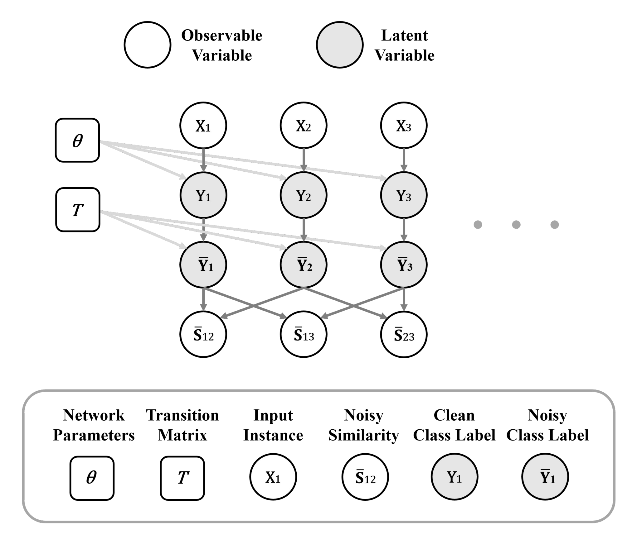
In this paper, we study the problem of how to learn a Multi-class classifier from Noisy-Similarity-labeled data, which is called MNS classification. Specifically, we assume that latent clean class labels flip into latent noisy labels , leading to noisy similarity labels . The corresponding graphical model, representing the interactions among variables, is shown in Figure 1. Based on this, we could further model the noise in the problem by using a transition matrix, i.e., represents the probabilities that the clean class label flips into the noisy class label and . We will show that under a mild assumption that anchor points ( defined in 3.3) exist in the training data, we can estimate the transition matrix by only employing noisy-similarity-labeled data. Then, we build a deep learning system for multi-class classification from only noisy-similarity-labeled data. Note that if a good classifier can be learned, the corresponding method can be easily extended to learn metrics or clusters, because accurate labels and similar and dissimilar pairs can be assigned by the good classifier. In other words, the proposed method can not only learn a classifier from noisy-similarity-labeled data but metrics and clusters. The contributions of this paper are summarized as follows:
- •
We propose a deep learning system for multi-class classification to address the problem of how to learn from noisy-similarity-labeled data.
- •
We propose to model the noise by using the transition matrix based on a graphical model. We show that the transition matrix can be estimated from only noisy-similarity-labeled data. The effectiveness will be verified on both synthetic and real data.
- •
We theoretically establish a generalization error bound for the proposed MNS classification method, showing that the learned classifier will generalize well on unseen data.
- •
We empirically demonstrate that the proposed method can effectively reduce the side effect of noisy-similarity-labeled data. It significantly surpasses the baselines on many datasets with both synthetic noise and real-world noise 11 1 Datasets with real-world noise refer the noisy-similarity-labeled data where noisy similarity labels are generated using real-world data with label noise..
The rest of this paper is organized as follows. In Section 2, we formalize the MNS classification problem, and in Section 3, we propose the MNS learning and practical implementation. Generalization error bound is analysed in Section 4. Experimental results are discussed in Section 5. We conclude our paper in Section 6.
2 Framing the MNS classification Problem
Problem setup. Let be the distribution of a pair of random variables , where and represents the dimension; is the label space and is the number of classes. Our goal is to predict a label for any given instance . Different from the traditional multi-class classification, in our setting, the class labels are not observable. Instead, we have noisy similarity labels . The clean similarity labels indicate the similarities between examples, i.e., where and denote the class labels for instances and . For noisy similarity labels, some of them are identical to the clean similarity labels, but some are different and we do not know which of them are clean. To the best of our knowledge, no existing work has discussed how to learn with the noisy similarity labels. We would like to review how the state-of-the-art work learns a classifier from the clean similarity labels.
MCL classification [Hsu et al. 2019]. Meta classification learning (MCL) utilizes the following likelihood to explain the similrity-based data
| (1) |
By introducing an independence assumption: [Hsu et al. 2019, Appendix D], in other words, and are independent to each other given and ; they can simplify the likelihood expression as
| (2) |
Then taking a negative logarithm on Equation 2, the final loss function can be derived as
| (3) |
where , which can be learned from a neural network.
However, class label noise is ubiquitous in our daily life [Kaneko et al. 2019, Hu et al. 2019b, Zhong et al. 2019b, Acuna et al. 2019, Lee et al. 2018, Tanaka et al. 2018, Wang et al. 2018], not to mention the weaker supervision: similarity labels. The performance of classifiers will get worse if we still use the state-of-the-art methods designed for clean similarity labels. This motivates us to find a novel algorithm for learning from noisy-similarity-labeled data.
3 MNS Learning
In this section, we propose a method for multi-class classification from noisy-similarity-labeled data.
3.1 Modeling noise in the supervision
To learn from the noisy-similarity-labeled data, we should model the noise. To model the noise, we introduce a graphic model in Figure 1 to describe the interactions among variables, where only input instances and noisy similarity labels are observed while both clean class labels and noisy class labels are latent. Rather than modeling the similarity-label noise directly, we assume that noise first occurs on latent class labels and as a consequence, similarity labels turn to noisy ones, i.e., noisy similarity labels indicate the similarities between noisy examples, and . The assumption is reasonable. For example, in the sensitive matters, to hide one’s thought on the question “With whom do you share the same opinion on issue A?”, people would like to randomly choose a fake opinion about the issue and answer the question conditioned on the fake opinion.
Specifically, to precisely describe label noise, we utilize a noise transition matrix [Cheng et al. 2017]. The transition matrix is generally dependent on instances, i.e., . Given only noisy examples, the instance-dependent transition matrix is non-identifiable without any additional assumption [Xia et al. 2019]. In this paper, we assume that given , is independent on instance and . This assumption considers the situations where noise relies only on the classes, which has been widely adopted in the class-label-noise learning community [Han et al. 2018, Xia et al. 2019]. Empirical results on real-datasets verify the efficiency of the assumptions.
We denote by the distribution of the noisy-similarity-labeled data , and the classifier is supposed to be learned from a training sample drawn from .

3.2 Likelihood-based estimator
Intuitively, according to figure 1, we can explain the noisy-similarity-based data by using the following likelihood model
| (4) |
In order to calculate the above likelihood, we have to marginalize the clean class label and noisy class label . Thanks to our proposed deep learning system (summarized in Figure 2), , modeled by a noise transition matrix , could be learned only from noisy data (shown in Section 3.3). Therefore, we only need to marginalize noisy class label . With the independence assumption , we can calculate the likelihood with the following expression
| (5) |
where the proportion relationship holds because is constant for given such that can be omitted. Note that
| (6) |
Let and , we have
| (7) |
Then by taking a negative logarithm on Equation 5 and substituting with , we obtain the objective function of the proposed method, i.e.,
| (8) |


Let us look inside Equation 8. Intuitively, outputs the predicted noisy categorical distribution of instance and is exactly the predicted noisy similarity, indicating the probability of data pairs belonging to the same noisy class. For clarity, we visualize the predicted noisy similarity in Figure 3. If and are predicted belonging to the same class, i.e., , the predicted noisy similarity should be relatively high ( in Figure 3(a)). By contrast, if and are predicted belonging to different classes, the predicted noisy similarity should be relatively low ( in Figure 3(b)).
Further, let , denoting the predicted noisy similarity. Substituting into Equation 8, can convert into a binary cross-entropy loss version, i.e.,
| (9) |
Let us look inside Equation 9. We could treat as the loss function denoting the loss of using to predict . Then, our problem can be formulated in the traditional risk minimization framework [Mohri et al. 2018]. The expected and empirical risks of employing estimator can be defined as
| (10) |
and
| (11) |
where is training sample size of the noisy-similarity-labeled data.
The whole pipeline is summarized in Figure 2. The softmax function outputs an estimator for the clean class posterior, i.e., , where denotes the estimated posterior. After the softmax layer, a noise transition matrix layer is added. According to Equation 7, by pre-multiplying the transpose of the transition matrix, we can obtain a predictor for the noisy class posterior, which can be further used to compute the prediction of the noisy similarity label, i.e., . Therefore, by minimizing , as the training data goes to infinity, will converge to noisy similarity and will converge to the optimal classifier for predicting noisy class labels. Meanwhile, given the true transition matrix, will converge to the optimal classifier for predicting clean class labels.
3.3 Estimate noise transition matrix
However, the transition matrix is unknown. We will discuss how to estimate the transition matrix for the noisy-similarity-labeled data in this subsection.
Anchor points [Liu and Tao 2015, Patrini et al. 2017, Yu et al. 2018] have been widely used to estimate the transition matrix for noisy-class-labeled data [Niu et al. 2018]. We illustrate that they can also be used to estimate the transition matrix for the noisy-similarity-labeled data. Specifically, an anchor point for class is defined as and , . Let be an anchor point for class such that and for . Then we have
| (12) |
Equation 3.3 shows that given anchor points for each class and the noisy class posterior distribution, the transition matrix can be estimated. Note that the noisy class posterior can be estimated by using the pipeline in Figure 2 without the transition matrix layer. However, it is a bit strong to have access to anchor points. Instead, we assume that anchor points exist in the training data but unknown to us. Empirically, we select examples with the highest as anchor points for the -th class.
3.4 Implementation
Given the true transition matrix, we can directly build a neural network as shown in Figure 2 to learn a multi-class classifier only from the noisy-similarity-labeled data. When the true transition matrix is unknown, we estimate it with the method proposed in Section 3.3 and then we can train the whole network as normal. The proposed algorithm is summarized in Algorithm 1.
Input: noisy-similarity-labeled training data; noisy-similarity-labeled validation data.
Stage 1: Learn
1: Learn by training the notwork in Figure 2 without the noise transition matrix layer;
2: Estimate according to Equation (3.3) by using instances with the highest as anchor points;
Stage 2: Learn the classifier
3: Fix the transition matrix layer in Figure 2 by using the estimated transition matrix;
4: Minimize to learn and stop when corresponds the minimum classification error on the noisy validation set;
Output: .
4 Generalization error
In this section, we will theoretically analyze the generalization ability of the proposed method. Although it looks complex, we will show that it will generalize well.
Assume that the neural network has layers with parameter matrices , and the activation functions are Lipschitz continuous, satisfying . We denote by the standard form of the neural network. Then the output of the softmax function is defined as , and is the output of the noise transition matrix layer. Let be the classifier learned from the hypothesis space determined by the neural network, i.e., . Note that the risks are defined in Section 3.2.
Theorem 1.
Assume the parameter matrices have Frobenius norm at most , and the activation functions are 1-Lipschitz, positive-homogeneous, and applied element-wise (such as the ReLU). Assume the transition matrix is given, and the instances are upper bounded by , i.e., for all X, and the loss function is upper bounded by 22 2 The assumption holds because deep neural networks will always regulate the objective to be a finite value and thus the corresponding loss functions are of finite values.. Then, for any , with probability at least ,
| (13) |
A detailed proof is provided in Appendix.
Theorem 1 implies that if the training error is small and the training sample size is large, the expected risk of the learned classifier for noisy classes will be small. If the transition matrix is well estimated, the learned classifier for the clean class will also have a small risk according to Equation 7. This theoretically justifies why the proposed method works well. In the experiment section, we will show that the transition matrices will be well estimated and that the proposed method will significantly outperform the baselines.
5 Experiments
In this section, we empirically investigate the performance of noise transition matrix estimation and the proposed method for MNS classification on three synthetic noisy datasets and two real-world noisy datasets.
5.1 Experiments on synthetic noisy datasets
Datasets. We synthesize noisy-similarity-labeled data by employing three widely used datasets, i.e., MNIST [LeCun 1998], CIFAR-10, and CIFAR-100 [Krizhevsky et al. 2009]. MNIST has grayscale images of 10 classes including 60,000 training images and 10,000 test images. CIFAR-10 and CIFAR-100 both have color images including 50,000 training images and 10,000 test images. CIFAR-10 has 10 classes while CIFAR-100 has 100 classes. For all the three benchmark datasets, we leave out 10% of the training examples as a validation set, which is for model selection.
Noisy similarity labels generation. First, we artificially corrupt the class labels of training and validation sets according to noise transition matrices. Specifically, for each instance with clean label , we replace its label by with a probability of . After that, we assign data pairs noisy similarity labels and remove and . In this paper, we consider the symmetric noisy setting defined in Appendix. Noise-0.5 generates severe noise which means almost half labels are corrupted while Noise-0.2 generates slight noise which means around 20% labels are corrupted.
Baselines. We compare our proposed method with state-of-the-art methods and conduct all the experiments with default parameters by PyTorch on NVIDIA Tesla V100. Specifically, we compare with the following two algorithms:
- •
Meta Classification Likelihood (MCL) [Hsu et al. 2019], which is the state-of-the-art method for multi-classification from clean-similarity-labeled data.
- •
KLD-based Contrastive Loss (KCL) [Hsu and Kira 2016], which is a strong baseline. It uses Kullback–Leibler divergence to mesure the distance between two distributions.
Network structure. For MNIST, we use LeNet. For CIFAR-10, we use pre-trained ResNet-32. For CIFAR-100, we use VGG8. For all networks, as shown in Figure 2, the output number of the last fully connected layer is set to be the number of classes. We add a noise transition matrix layer after the softmax. Since the loss functions of MNS, MCL and KCL are designed for instance pairs, a pairwise enumeration layer [Hsu et al. 2018] is adapted before calculating the loss.
Optimizer. We follow the optimization method in [Patrini et al. 2017] to learn the noise transition matrix . To learn , we use the Adam optimizer with initial learning rate 0.001. On MNIST, the batch size is 128 and the learning rate decays every 10 epochs by a factor of 0.1 with 30 epochs in total. On CIFAR-10, the batch size is also 128 and the learning rate decays every 40 epochs by a factor of 0.1 with 120 epochs in total. On CIFAR-100, the batch size is 1000 and the learning rate drops at epoch 80 and 160 by a factor of 0.1 with 200 epochs in total.
| Noise | 0.2 | 0.3 | 0.4 | 0.5 | 0.6 |
|---|---|---|---|---|---|
| KCL | 99.200.02 | 99.060.05 | 95.973.65 | 90.610.78 | 85.204.69 |
| MCL | 98.510.10 | 98.280.06 | 97.920.24 | 97.540.09 | 96.940.20 |
| MNS() | 98.560.07 | 98.290.16 | 98.010.15 | 97.610.41 | 97.260.23 |
| MNS() | 98.750.07 | 98.690.11 | 98.320.09 | 98.180.13 | 94.484.49 |
| Noise | 0.2 | 0.3 | 0.4 | 0.5 | 0.6 |
|---|---|---|---|---|---|
| KCL | 19.141.27 | 17.672.15 | 18.581.28 | 17.963.41 | 15.141.67 |
| MCL | 75.583.64 | 68.900.32 | 63.381.32 | 61.670.98 | 44.552.96 |
| MNS() | 78.831.81 | 76.801.33 | 70.351.21 | 68.870.97 | 50.992.88 |
| MNS() | 82.420.37 | 77.420.46 | 70.710.33 | 69.280.41 | 40.240.61 |
| Noise | 0.2 | 0.3 | 0.4 | 0.5 | 0.6 |
|---|---|---|---|---|---|
| KCL | 13.321.57 | 7.9820.57 | 5.4060.15 | 3.7380.45 | 3.2080.55 |
| MCL | 48.380.38 | 40.480.79 | 32.750.77 | 26.480.36 | 21.940.19 |
| MNS() | 48.780.74 | 43.900.39 | 40.260.93 | 35.140.69 | 31.400.26 |
| MNS() | 51.950.44 | 48.970.25 | 46.451.00 | 42.010.78 | 36.500.45 |
Results. The results in Tables 1, 2, and 3 demonstrate the test accuracy and stability of four algorithms on three benchmark datasets. Overall, we can see that when similarity labels are corrupted, MNS() achieves the best performance among three similarity-based learning methods, approaching or even exceeding MNS() which is given the true noise transition matrix. Specifically, On MNIST and CIFAR10, when the noise rates are high, MNS() performs better than MNS(). This should because that and the networks are learned jointly as shown in Algorithm 1.
On MNIST, when the noise rate is relatively low (under 0.4), KCL has the highest accuracy; MCL and MNS also perform well. Intuitively, compared with inner product, Kullback-Leibler divergence measures the similarity between two distributions better, but it may introduce bad local minima or small gradients for learning [Hsu et al. 2019] such that it has poor performances on more complex datasets or higher noise rate. For example, when the noise rate increases (beyond 0.3), the accuracy of KCL drops dramatically, falling form 99.06 at Noise-0.3 to 85.20 at Noise-0.6. By contrast, MNS and MCL are more robust to noise. Both methods decrease slightly as the noise rate rises while our method is always a little better than the state-of-the-art method MCL.
On CIFAR-10 and CIFAR-100, there is a significant decrease in the accuracy of all methods and our method achieves the best results across all noise rate, i.e., at Noise-0.6, MNS gives an accuracy uplift of about 6.5% and 10% on CIFAR-10 and CIFAR-100 respectively compared with the state-of-the-art method MCL.
5.2 Experiments on real-world noisy datasets
Datasets. We verify the effectiveness of the proposed method on two real-word datasets with noisy supervision, i.e., Clothing1M [Xiao et al. 2015] and Food-101 [Bossard et al. 2014]. Specifically, Clothing1M has 1M images with real-world noisy labels and additional 50k, 14k, 10k images with clean labels for training, validation and testing. We only use noisy training set in training phase and leave out 10% as validation set for model selection and test our model on 10k testing set. Food-101 consists of 101 food categories, with 101,000 images. For each class, 250 manually reviewed clean test images are provided as well as 750 training images with real-world noise. For Food-101, we also leave out 10% for validation. In particular, we use Random Crop and Random Horizontal Flip for data augmentation. Since datasets contain some amount of class label noise already, we do not need to corrupt the labels artificially. We generate noisy-similarity-labeled data by using the noisy-class-labeled data directly.
Baselines. The same as the synthetic experiment part.
Network structure and optimizer. For all experiments, we use pre-trained ResNet-50. On Clothing1M, the batch size is 256 and the learning rate drops every 5 epochs by a factor of 0.1 with 10 epochs in total. On Food-101, the batch size is 1000 and the learning rate drops at epoch 80 and 160 by a factor of 0.1 with 200 epochs in total. Other settings are the same as the synthetic experiment part.
| KCL | MCL | MNS() |
|---|---|---|
| 9.49 | 66.20 | 67.50 |
| KCL | MCL | MNS() |
|---|---|---|
| 30.17 | 48.08 | 71.18 |
Results. From Table 4 and 5, We can see that on Clothing1M, MNS() achieves the best accuracy. On Food-101, MNS() also performs distinguishedly, uplifting about 23% in accuracy compared with MCL. Specifically, the gap between MCL and MNS() is huge in Table 5 while is not in Table 4. Let us review the definition of similarity-labeled data: if two instances belong to the same class, they will have similarity label , otherwise . That is to say, for a -class dataset, only around of similarity-labeled data has similarity labels , and the rest has similarity labels . For Clothing1M (Table 4), the . For Food-101 (Table 5), the . Therefore, the generated similarity-labeled data from Food-101 is much more unbalanced than that from Clothing1M. As a result, the baseline performed badly on Food-101, making the gap huge in Table 5.
5.3 Noise transition matrix estimation
To estimate , we first learn the noisy predictor . For each dataset, the network and optimizer remain the same as above but the noise transition matrix layer is exclude. is then estimated using the method proposed in Section 3.3.


Here we only show the estimated transition matrices of three synthetic noisy datasets because we have the exact values of the true transition matrices such that we could assess the estimation accuracies. Estimated transition matrices of real-world noisy datasets are provided in Appendix. From Figure 4 and 5, we can see that transition matrices estimated with the proposed method are very close to the true one. By employing the calculation method of estimation error as , MNIST, CIFAR-10 and CIFAR-100 achieve 0.0668, 0.1144 and 0.1055 in error respectively.
6 Conclusion
This paper proposes a noisy-similarity-based multi-class classification algorithm (called MNS classification) by designing a novel deep learning system exploiting only noisy-similarity-labeled data. MNS classification provides an effective way for making predictions on sensitive matters where it is difficult to collect high-quality data such that similarities with noise could be all the information available. The core idea is to model the noise in the latent noisy class labels by using a noise transition matrix while only noisy similarity labels are observed. By adding a noise transition matrix layer in the deep neural network, it turns to robust to similarity label noise. We also present that noise transition matrix can be estimated in this setting. Experiments are conducted on benchmark-simulated and real-world label-noise datasets, demonstrating our method can excellently solve the above weakly supervised problem. In future work, investigating different types of noise for diverse real-life scenarios might prove important.
References
- Acuna et al. [2019] David Acuna, Amlan Kar, and Sanja Fidler. Devil is in the edges: Learning semantic boundaries from noisy annotations. In Proceedings of the IEEE Conference on Computer Vision and Pattern Recognition, pages 11075–11083, 2019.
- Bao et al. [2018] Han Bao, Gang Niu, and Masashi Sugiyama. Classification from pairwise similarity and unlabeled data. In International Conference on Machine Learning, pages 461–470, 2018.
- Bartlett and Mendelson [2002] Peter L Bartlett and Shahar Mendelson. Rademacher and gaussian complexities: Risk bounds and structural results. Journal of Machine Learning Research, 3(Nov):463–482, 2002.
- Bossard et al. [2014] Lukas Bossard, Matthieu Guillaumin, and Luc Van Gool. Food-101 – mining discriminative components with random forests. In European Conference on Computer Vision, 2014.
- Cheng et al. [2017] Jiacheng Cheng, Tongliang Liu, Kotagiri Ramamohanarao, and Dacheng Tao. Learning with bounded instance-and label-dependent label noise. arXiv preprint arXiv:1709.03768, 2017.
- Golowich et al. [2017] Noah Golowich, Alexander Rakhlin, and Ohad Shamir. Size-independent sample complexity of neural networks. arXiv preprint arXiv:1712.06541, 2017.
- Han et al. [2018] Bo Han, Quanming Yao, Xingrui Yu, Gang Niu, Miao Xu, Weihua Hu, Ivor Tsang, and Masashi Sugiyama. Co-teaching: Robust training of deep neural networks with extremely noisy labels. In Advances in neural information processing systems, pages 8527–8537, 2018.
- Han et al. [2019] Jiangfan Han, Ping Luo, and Xiaogang Wang. Deep self-learning from noisy labels. In Proceedings of the IEEE International Conference on Computer Vision, pages 5138–5147, 2019.
- Hsu and Kira [2016] Yen-Chang Hsu and Zsolt Kira. Neural network-based clustering using pairwise constraints. In ICLR workshop, 2016. URL https://arxiv.org/abs/1511.06321.
- Hsu et al. [2018] Yen-Chang Hsu, Zhaoyang Lv, and Zsolt Kira. Learning to cluster in order to transfer across domains and tasks. In International Conference on Learning Representations (ICLR), 2018. URL https://openreview.net/forum?id=ByRWCqvT-.
- Hsu et al. [2019] Yen-Chang Hsu, Zhaoyang Lv, Joel Schlosser, Phillip Odom, and Zsolt Kira. Multi-class classification without multi-class labels. arXiv preprint arXiv:1901.00544, 2019.
- Hu et al. [2019a] Mengying Hu, Hu Han, Shiguang Shan, and Xilin Chen. Weakly supervised image classification through noise regularization. In Proceedings of the IEEE Conference on Computer Vision and Pattern Recognition, pages 11517–11525, 2019a.
- Hu et al. [2019b] Wei Hu, Yangyu Huang, Fan Zhang, and Ruirui Li. Noise-tolerant paradigm for training face recognition cnns. In Proceedings of the IEEE Conference on Computer Vision and Pattern Recognition, pages 11887–11896, 2019b.
- Kaneko et al. [2019] Takuhiro Kaneko, Yoshitaka Ushiku, and Tatsuya Harada. Label-noise robust generative adversarial networks. In Proceedings of the IEEE Conference on Computer Vision and Pattern Recognition, pages 2467–2476, 2019.
- Khetan et al. [2017] Ashish Khetan, Zachary C Lipton, and Anima Anandkumar. Learning from noisy singly-labeled data. arXiv preprint arXiv:1712.04577, 2017.
- Krause et al. [2016] Jonathan Krause, Benjamin Sapp, Andrew Howard, Howard Zhou, Alexander Toshev, Tom Duerig, James Philbin, and Li Fei-Fei. The unreasonable effectiveness of noisy data for fine-grained recognition. In European Conference on Computer Vision, pages 301–320. Springer, 2016.
- Krizhevsky et al. [2009] Alex Krizhevsky, Geoffrey Hinton, et al. Learning multiple layers of features from tiny images. Technical report, Citeseer, 2009.
- LeCun [1998] Yann LeCun. The mnist database of handwritten digits. http://yann. lecun. com/exdb/mnist/, 1998.
- Ledoux and Talagrand [2013] Michel Ledoux and Michel Talagrand. Probability in Banach Spaces: isoperimetry and processes. Springer Science & Business Media, 2013.
- Lee et al. [2018] Kuang-Huei Lee, Xiaodong He, Lei Zhang, and Linjun Yang. Cleannet: Transfer learning for scalable image classifier training with label noise. In Proceedings of the IEEE Conference on Computer Vision and Pattern Recognition, pages 5447–5456, 2018.
- Li et al. [2018] Chenglong Li, Chengli Zhu, Yan Huang, Jin Tang, and Liang Wang. Cross-modal ranking with soft consistency and noisy labels for robust rgb-t tracking. In Proceedings of the European Conference on Computer Vision (ECCV), pages 808–823, 2018.
- Li et al. [2019] Junnan Li, Yongkang Wong, Qi Zhao, and Mohan S Kankanhalli. Learning to learn from noisy labeled data. In Proceedings of the IEEE Conference on Computer Vision and Pattern Recognition, pages 5051–5059, 2019.
- Li et al. [2017] Yuncheng Li, Jianchao Yang, Yale Song, Liangliang Cao, Jiebo Luo, and Li-Jia Li. Learning from noisy labels with distillation. In Proceedings of the IEEE International Conference on Computer Vision, pages 1910–1918, 2017.
- Li and Liu [2009] Zhenguo Li and Jianzhuang Liu. Constrained clustering by spectral kernel learning. In 2009 IEEE 12th International Conference on Computer Vision, pages 421–427. IEEE, 2009.
- Liu and Tao [2015] Tongliang Liu and Dacheng Tao. Classification with noisy labels by importance reweighting. IEEE Transactions on pattern analysis and machine intelligence, 38(3):447–461, 2015.
- Mohri et al. [2018] Mehryar Mohri, Afshin Rostamizadeh, and Ameet Talwalkar. Foundations of Machine Learning. MIT Press, 2018.
- Niu et al. [2014] Gang Niu, Bo Dai, Makoto Yamada, and Masashi Sugiyama. Information-theoretic semi-supervised metric learning via entropy regularization. Neural computation, 26(8):1717–1762, 2014.
- Niu et al. [2018] Li Niu, Qingtao Tang, Ashok Veeraraghavan, and Ashutosh Sabharwal. Learning from noisy web data with category-level supervision. In Proceedings of the IEEE Conference on Computer Vision and Pattern Recognition, pages 7689–7698, 2018.
- Patrini et al. [2017] Giorgio Patrini, Alessandro Rozza, Aditya Krishna Menon, Richard Nock, and Lizhen Qu. Making deep neural networks robust to label noise: A loss correction approach. In Proceedings of the IEEE Conference on Computer Vision and Pattern Recognition, pages 1944–1952, 2017.
- Shimada et al. [2019] Takuya Shimada, Han Bao, Issei Sato, and Masashi Sugiyama. Classification from pairwise similarities/dissimilarities and unlabeled data via empirical risk minimization. arXiv preprint arXiv:1904.11717, 2019.
- Tanaka et al. [2018] Daiki Tanaka, Daiki Ikami, Toshihiko Yamasaki, and Kiyoharu Aizawa. Joint optimization framework for learning with noisy labels. In Proceedings of the IEEE Conference on Computer Vision and Pattern Recognition, pages 5552–5560, 2018.
- Tanno et al. [2019] Ryutaro Tanno, Ardavan Saeedi, Swami Sankaranarayanan, Daniel C Alexander, and Nathan Silberman. Learning from noisy labels by regularized estimation of annotator confusion. arXiv preprint arXiv:1902.03680, 2019.
- Wagstaff et al. [2001] Kiri Wagstaff, Claire Cardie, Seth Rogers, Stefan Schrödl, et al. Constrained k-means clustering with background knowledge. In Icml, volume 1, pages 577–584, 2001.
- Wang et al. [2018] Yisen Wang, Weiyang Liu, Xingjun Ma, James Bailey, Hongyuan Zha, Le Song, and Shu-Tao Xia. Iterative learning with open-set noisy labels. In Proceedings of the IEEE Conference on Computer Vision and Pattern Recognition, pages 8688–8696, 2018.
- Wang et al. [2019] Yisen Wang, Xingjun Ma, Zaiyi Chen, Yuan Luo, Jinfeng Yi, and James Bailey. Symmetric cross entropy for robust learning with noisy labels. In Proceedings of the IEEE International Conference on Computer Vision, pages 322–330, 2019.
- Xia et al. [2019] Xiaobo Xia, Tongliang Liu, Nannan Wang, Bo Han, Chen Gong, Gang Niu, and Masashi Sugiyama. Are anchor points really indispensable in label-noise learning? arXiv preprint arXiv:1906.00189, 2019.
- Xiao et al. [2015] Tong Xiao, Tian Xia, Yi Yang, Chang Huang, and Xiaogang Wang. Learning from massive noisy labeled data for image classification. In Proceedings of the IEEE conference on computer vision and pattern recognition, pages 2691–2699, 2015.
- Xing et al. [2003] Eric P Xing, Michael I Jordan, Stuart J Russell, and Andrew Y Ng. Distance metric learning with application to clustering with side-information. In Advances in neural information processing systems, pages 521–528, 2003.
- Yi and Wu [2019] Kun Yi and Jianxin Wu. Probabilistic end-to-end noise correction for learning with noisy labels. arXiv preprint arXiv:1903.07788, 2019.
- Yu et al. [2018] Xiyu Yu, Tongliang Liu, Mingming Gong, and Dacheng Tao. Learning with biased complementary labels. In Proceedings of the European Conference on Computer Vision (ECCV), pages 68–83, 2018.
- Zhang et al. [2016] Chiyuan Zhang, Samy Bengio, Moritz Hardt, Benjamin Recht, and Oriol Vinyals. Understanding deep learning requires rethinking generalization. arXiv preprint arXiv:1611.03530, 2016.
- Zhang et al. [2018] Jing Zhang, Tong Zhang, Yuchao Dai, Mehrtash Harandi, and Richard Hartley. Deep unsupervised saliency detection: A multiple noisy labeling perspective. In Proceedings of the IEEE Conference on Computer Vision and Pattern Recognition, pages 9029–9038, 2018.
- Zhang et al. [2019] Weihe Zhang, Yali Wang, and Yu Qiao. Metacleaner: Learning to hallucinate clean representations for noisy-labeled visual recognition. In Proceedings of the IEEE Conference on Computer Vision and Pattern Recognition, pages 7373–7382, 2019.
- Zhong et al. [2019a] Jia-Xing Zhong, Nannan Li, Weijie Kong, Shan Liu, Thomas H Li, and Ge Li. Graph convolutional label noise cleaner: Train a plug-and-play action classifier for anomaly detection. In Proceedings of the IEEE Conference on Computer Vision and Pattern Recognition, pages 1237–1246, 2019a.
- Zhong et al. [2019b] Yaoyao Zhong, Weihong Deng, Mei Wang, Jiani Hu, Jianteng Peng, Xunqiang Tao, and Yaohai Huang. Unequal-training for deep face recognition with long-tailed noisy data. In Proceedings of the IEEE Conference on Computer Vision and Pattern Recognition, pages 7812–7821, 2019b.
- Zhou [2017] Zhi-Hua Zhou. A brief introduction to weakly supervised learning. National Science Review, 5(1):44–53, 2017.
Appendices
Appendix A Proof of Theorem 1
We have defined
| (14) |
and
| (15) |
where is training sample size of the noisy-similarity-labeled data.
First we bound the generalization error with Rademacher complexity [3].
Theorem 2 ([3]).
Let the loss function be upper bounded by . Then, for any , with the probability , we have
| (16) |
where is the Rademacher complexity defined by
| (17) |
and are Rademacher variables uniformly distributed from .
Before further upper bound the Rademacher complexity , we discuss the special loss function and its Lipschitz continuity w.r.t .
Lemma 1.
Given transition matrix , loss function is 1-Lipschitz with respect to ,
| (18) |
Based on Lemma 1, we can further upper bound the Rademacher complexity by the following lemma.
Lemma 2.
Given transition matrix and assume loss function is 1-Lipschitz with respect to , we have
| (19) |
where is the function class induced by the deep neural network.
The right hand part of the above inequality, indicating the hypothesis complexity of deep neural networks, can be bound by the following theorem.
Theorem 3 ([6]).
Assume the Frobenius norm of the weight matrices are at most . Let the activation functions be 1-Lipschitz, positive-homogeneous, and applied element-wise (such as the ReLU). Let is upper bounded by B, i.e., for any , . Then,
| (20) |
A.1 Proof of Lemma 1
Recall that
| (21) |
where
| (22) |
Take the derivative of w.r.t. , we have
| (23) |
where
Note that the derivative of the softmax function has some properties, i.e., if , and if , .
A.2 Proof of Lemma 2
where the first three equations hold because given , and give the same constraint on ; the sixth inequality holds because of the Lemma [19].
Appendix B Definition of transition matrix
Symmetric noisy setting is defined as follows, where C is the number of classes.
| Noise-: | (30) |
Appendix C Estimation of transition matrix on real-world noisy datasets
Here we show the estimated transition matrices of Clothing1M and the first ten classes of Food-101. For Clothing1M, we use additional 50k images with clean labels to learn the transition matrix such that the left in Figure 1 is very close to the true one. The right in Figure 1 was estimated only from noisy-similarity-labeled data, which learned most of the features of true transition matrix. For Food-101, both was estimated from noisy-labeled data. From Figure 2 we can see that the result close to the result which verifies the effectiveness of our method.

