Exponential of the Trace of the Free Field and Verblunsky Coefficients
Abstract.
An identity of Szego, and a volume calculation, heuristically suggest a simple expression for the distribution of Verblunsky coefficients with respect to the (normalized) exponential of the trace of the Gaussian free field. This heuristic expression is not quite correct. A proof of the correct formula has been found by Chhaibi and Najnudel ([5]). Their proof uses random matrix theory and overcomes many difficult technical issues. In addition to presenting the Szego perspective, we show that the Chhaibi and Najnudel theorem implies a family of combinatorial identities (for moments of measures) which are of intrinsic interest.
0. Introduction
Let denote the metrizable compact convex set of probability measures on the unit circle with the weak* topology, let denote the subset consisting of measures with infinite support, and let . The Verblunsky correspondence refers to a miraculous homeomorphism
| (0.1) |
or more generally to a homeomorphism of and a compactification of the product space. This correspondence can be described in several different ways. One formulation is as follows. Given , if , , ,… are the monic orthogonal polynomials corresponding to , then (where is complex conjugation). Conversely, given , is the weak* limit of probability measures
| (0.2) |
where ,
| (0.3) |
and (our conventions for Verblunsky coefficients differ slightly from those in [13], see Subsection 0.2). In the text we will use a reformulation of Szego’s recursion (0.3) which relates Verblunsky coefficients to root subgroup coordinates for the loop group .
Suppose that and write
where is perpendicular to the Lebesgue class. A famous theorem of Szego asserts that if , then
| (0.4) |
In Section 4 we will see that for finite ,
| (0.5) |
where is the characteristic function for the image of the map and denotes Lebesgue measure. Let
| (0.6) |
At a heuristic level, the identities (0.4) and (0.5) suggest that
| (0.7) |
where there is a notable shift of exponent , and is a conditioning on the left hand side (which, to give the story away, reduces the statement to ).
The measures , , can be characterized in many different ways. For example they exhaust all of the conformally invariant Gaussian distributions for , where . In terms of boundary values, where is interpreted as a real hyperfunction modulo constants, is the (normalized) trace of the Gaussian free field with inverse temperature . From this latter point of view, a notorious complication is that the hyperfunction is -almost surely not an ordinary function on the circle. Consequently the naive map in which a (normalized) real valued function is mapped to the Lebesgue class probability measure is defined on a set of -measure zero. However, from various points of view, it is well-known how to make sense of the map from (or ) to a probability measure in a -almost sure sense; we denote this map by . The following is a corollary of the work of Chhaibi and Najnudel ([5]).
Theorem 0.1.
Suppose that . Then
(where denotes pushforward of measures).
Thus (0.7) does correctly predict (at a heuristic level) that Verblunsky coefficients are independent, but the shift in parameter in (0.7) is misleading! The restriction on is very likely artificial, but for lack of expertise, we do not see how to dispense with it.
To prove this theorem it would suffice to show that for given , the two measures in Theorem 0.1 have the same distribution. The distribution is
| (0.8) |
Now consider and the measure
Using the Szego and volume identities (0.4) and (0.5), we can express this in terms of as
(where there is a straightforward but complicated way to express as a function of for ). Unfortunately it is not clear, even at a heuristic level, how to integrate out the intermediate variables and evaluate the resulting distribution in the limit as . Why is the limit conformally invariant? Why is it Gaussian? This is rather mysterious.
Modulo a number of important details, we will study the inverse of , as realized in the following diagram:
| (0.9) |
(in a deterministic context, one must restrict the domains, see Section 2; in the present probabilistic context, the map and its inverse are defined in almost sure senses). The first step in [5], depending crucially on random matrix theory, is essentially to show that
| (0.10) |
(where slightly abusing notation, on the left, , and on the right ). In terms of moments, this is equivalent to a set of identities (see Theorem 6.2) which are of intrinsic interest. For example the equality of expected values for is equivalent to
| (0.11) |
where the sum is over all integral sequences satisfying , for some . We do not have a conceptual explanation for the appearance of the probability mass function for a harmonic sequence of independent Bernoulli random variables.
At a heuristic level, the moment identities (which have the virtue of being computable), (0.10), and Theorem 0.1 are essentially equivalent; consequently the moment identities are well-worth understanding (see [8]). However at a technical level, because of the non-continuous nature of the map , there is a gap between (0.10) and Theorem 0.1; this is the void which [5] has filled. It would be highly desirable to understand this using softer techniques.
0.1. Plan of the Paper
The first three sections recall standard facts, albeit in slightly idiosyncratic ways. In Section 1 we recall why is the essentially unique conformally invariant Gaussian probability measure on , and why it is necessary to regularize the map . In Section 2 we show that Verblunsky coefficients are related to root subgroup coordinates for the loop group of , and we explain the deterministic meaning of the diagram (0.9). In Section Definition we explain how to properly formulate the map . In Section 4 we prove the volume formula (0.5). In Sections 5 and 6 we calculate moments for the coefficients of with respect to the and -distributions (in Theorem 0.1), respectively. (0.10) is equivalent to the equality of these two calculations, as formulated in Theorem 6.2. In [8] our goal is to give direct proofs of these identities, but as of this writing, this remains a goal.
0.2. Notation
Our conventions regarding Verblunsky coefficients differ from those in [13], where the nontrivial coefficients are indexed by . We use the convention that and the nontrivial Verblunsky coefficients are . The rationale is that the group of rotations of the circle acts naturally on , and the map to Verblunsky coefficients is equivariant provided that rotation by acts on (in our notation) by . We also switch the sign of the coefficients. Thus our is the negative of the th coefficient in [13]. This eliminates a profusion of signs that would appear otherwise.
1. Background
The group acts on the open unit disk by linear fractional transformations,
| (1.1) |
This identifies with the group of all conformal automorphisms of , or equivalently with the group of all orientation-preserving isometries of , equipped with the non-Euclidean arclength . For this metric the Gaussian curvature , and the global metric on is given by
| (1.2) |
The action of on induces an action (by pullback) on , the space of holomorphic differentials of order , for . The action of on is
| (1.3) |
The space is a Frechet space with respect to the topology of uniform convergence on compact sets, and the action is continuous. More generally the universal covering acts on for any .
For each , the action contains an essentially unique irreducible unitary action (This is proven by considering the (lowest weight) infinitesimal action of the Lie algebra of , see e.g. [7]). If , then the invariant Hilbert norm is given by an integral
| (1.4) |
where and is the Beta function. We inserted the seemingly unnatural factor because the last sum shows that this norm can be analytically continued to , since .
Proposition 1.
Fix . For each , is an ergodic -invariant Gaussian measure. Conversely, if is an ergodic conformally invariant Gaussian on , then for some .
Proof.
The ergodicity of is a special case of a general result of Irving Segal, see [10]. The second statement follows from the fact that the unitary substructure for the action on is essentially unique and irreducible, see e.g. [7]. This determines the Cameron-Martin subspace for the Gaussian, hence determines the measure. For a completely different geometric proof, see [14]. ∎
We are primarily interested in the limit , which is exceptional. The action of on is reducible: is an invariant subspace. The norm as defined by (1.4) is not well-defined when . However, in the definition of the norm, we can multiply by . In this case we obtain a Hilbert space substructure for the quotient (the original vacuum, the constant , is now a ‘ghost’), and an isometry induced by the -equivariant Frechet space isomorphism
| (1.5) |
To set our notation, for
If , then ,
Define as in (0.6). If , then is the unique conformally invariant convolution semigroup of Gaussian measures on the spaces in (1.5). The almost sure properties of the associated random functions are considered in detail in [6], which we merely note for motivation. As random series , and
| (1.6) |
where are standard normal complex random variables. This is the critical case in chapter 13 of [6].
Proposition 2.
(a) Fix an angle . For all , almost surely
i.e. for each ray the image is almost surely dense in .
(b) Again fix the angle . Then almost surely
where .
Question.
Is (a) true for any ergodic conformally invariant , ?
2. Root Subgroup Coordinates
In this section we slightly reformulate the Szego recursion and observe that Verblunsky coefficients are related to so called root subgroup coordinates for loops into . This reformulation is surely not new. In fact the point is that in developing the theory of root subgroup factorization, the second author should have observed early on that some aspects had already been developed in the Verblunsky context.
2.1. Reformulation of the Szego Recursion
The Szego recursion can be written as
Consequently there is a closed formula
This does not have any meaning in the limit as .
Define the th reversed polynomial to be . Note that and (0.2) is equivalent to
| (2.1) |
because on the circle . The point of what follows is that we can take limits for the .
Lemma 1.
In terms of reversed polynomials, the Szego recursion (0.3) is equivalent to
Note that
is a loop with values in . A loop of this form has two properties. First, it has the form
where and are polynomials of degree satisfying and . Second, it has a triangular factorization (essentially a Riemann-Hilbert factorization)
where the first matrix is holomorphic in and at , is a positive constant, and the third matrix is a holomorphic map and unipotent upper triangular at . These two properties are equivalent (see [4]).
Instead of (and its root subgroup factorization), we are more interested in the matrix (and its root subgroup factorization) which appears in the Szego recursion
This is , except that we have dropped the numerical factors which enforce the algebraic condition (which is an implicit regularization). Note that in Lemma 1
| (2.2) |
Whereas the zeroes of are in , the zeroes of are in , the complement of the closed unit disk. This implies , because for a Verblunsky sequence with , , , , hence the limit in (2.1) is expressed exactly in terms of . To summarize, for Verblunsky sequences with a finite number of nonvanishing terms, the deterministic sense in which the diagram (0.9) inverts is that there are bijective correspondences
| (2.3) |
By taking limits (for functions and measures having smooth boundary values), this implies
Proposition 3.
The diagram (0.9) inverts when the and ’s are smooth up to the boundary, the sequences are rapidly decreasing, and the measures have smooth positive densities on the circle.
The Szego identity (0.3) implies that more generally the diagram is valid for and with and such that (There are also deterministic statements which apply to sequences, such as the ‘Szego condition’, see [12] and [13]). However none of this is applicable for the random that occur in Theorem 0.1.
For the purposes of this paper, it is crucial that there are simple explicit expressions for the coefficients of in terms of . By convention, in the following statement, . The following is a straightforward calculation.
Lemma 2.
For rapidly decreasing sequences of Verblunsky coefficients, , and , is the sum of terms of the form
for some , where the indices satisfy the constraints
For example
In general each is a multilinear function of the and their conjugates. By contrast each is a polynomial in the coefficients of .
The following definition is intended to capture basic intuition about the sum defining in terms of .
Definition.
The bulk terms in the sum for in Lemma 2 are those for which the all the gaps , i.e. those for which the length . Terms for which are referred to as boundary terms. We refer to a pair (with gap 1) as a 2-bit. In general we refer to a pair as an -bit.
Note that boundary terms arise when two or more 2-bits collide to form an -bit, where . For example the -bits and collide when , to form the -bit , where we think of and as annihilating one another in the process. This annihilation, or cancelation, process will play a central role in this paper.
3. Definition of the Map M
The main point of this section is to properly formulate the map in (0.9).
Given a point , there is an isometry
where , the sphere centered at with radius , is equipped with the induced non-Euclidean metric normalized to have length (the non-normalized length is ) (see (1.2)).
Let denote the set of all compact subsets of ; equipped with the Vietoris topology, is a metrizable compact Hausdorff space.
Define by
and let
Lemma 3.
Suppose . Then
(a)
(b)
(c)
(d) is stable with respect the action of .
(e) If , then is -almost surely a point iff for each , is -almost surely a point.
(f) If as in (e) is ergodic, then the measure of is zero or one.
Proof.
(b) asserts that , as a function of and a basepoint, is invariant. The other parts are consequences of this.
∎
From now on we will fix the basepoint , which will break -invariance.
Definition.
is defined by , i.e.
Remark.
This is a nonlocal regularization. In physics it is important that the regularization of is local. One can fairly ask why we are deviating from the local multiplicative chaos regularization; the answer is that we have stumbled on this point of view in other contexts, and this leads to interesting questions.
Since it is expressed as a limit, is a Borel map. However, is not continuous, and it is not -equivariant in any sense that we can identify (see Theorem 3.1 below). Despite all these shortcomings, it is a very interesting map (we will consider some of its deterministic properties elsewhere).
It follows from (f) of Lemma 3 that if is an ergodic -invariant distribution on , then is zero or one. There is an enormous variety of such measures, and for some is zero and for others it is one.
Proposition 4.
For , .
The proposition is a corollary of difficult but well-known facts from the theory of multiplicative chaos (For recent expositions, see section 3.3 of [1] or Theorem 1.3 of [5] (i.e. Theorem 1.2 of [2]) and the subsequent commentary (Our notation is consistent with the first reference and at odds with the second). As in the statement of Theorem 0.1, our nonlocal regularization probably makes the restriction on unnecessary, but we have failed to resolve this.
There exists a large (possibly intractable) family of invariant distributions on . This should be contrasted with the following
Theorem 3.1.
There does not exist a invariant probability measure on .
Proof.
Suppose otherwise. Then there exists an ergodic invariant probability measure. Relative to this ergodic measure, for a.e. , is dense in . We claim that the weak∗ closure of is the union of and the set of measures around the circle. This will imply that the orbit is not weak∗ dense, a contradiction.
There exists a point with . Given ,
is a hyperbolic element of with a repelling fixed point at and an attracting fixed point at . The limit of the measures tends to as . By applying a rotation if necessary, we can arrange for the limit to be any delta measure around the circle. Thus the delta measures are in the closure of the orbit through .
Conversely suppose that is in the closure of . There exists a sequence such that converges weakly to . For each let denote a fixed point for . By passing to a subsequence if necessary, we can suppose that .
If , then we can suppose . A subsequence of the will then converge to a rotation. In this case is just a rotation of and we are done.
So suppose that . In this event it is convenient to switch to the upper half space with .
By passing to a subsequence if necessary, we can suppose all of the are parabolic, or all of the are hyperbolic. In the parabolic case the are essentially horizontal translations. If there is a finite limit, then converges to a parabolic element. Otherwise is the delta measure at .
Suppose the are hyperbolic. Each has a second fixed point . By passing to a subsequence we can suppose this second sequence converges. Suppose these second fixed points converge to . Then we are essentially back in the parabolic case.
Suppose that the converge to a second point on the circle. We can suppose this second point is (in the upper half plane model). In this event the are dilations. If there is a finite limit for the magnitude of dilations, then the converge to a hyperbolic element and is in the orbit of . If for some subsequence, the magnitude goes to zero or one, then is a delta measure at either or .
This completes the proof.
∎
Corollary 1.
There does not exist a invariant probability measure on , where acts by composition on the right (where is identified with rotations and homeomorphisms are assumed to be orientation preserving).
Proof.
There is a equivariant isomorphism
(given a homeomorphism, the generalized derivative divided by is a probability measure, and given an atomless probability measure with full support, the corresponding cumulative distribution function (unique up to a shift) is a homeomorphism). Thus the corollary follows from the theorem. ∎
4. Volume Using Root Subgroup Factorization
In this section we use the notation established in Section 2. Throughout we fix , and by convention, .
Lemma 4.
The map
where , is an injective map onto an open domain properly contained in
Proof.
Abbreviate . First note that is nonvanishing. This is because is the th reversed polynomial for the measure corresponding to .
We now show that the map is injective. Given mapping to , we obtain a corresponding and a measure corresponding to . So the map is injective. The fact that the map is an injective polynomial map implies that the derivative is injective. This implies that the image is open. Since the are bounded by one, the image is bounded, hence it is properly contained in the set of which are nonvanishing in the closure of (Unfortunately it is not clear how to precisely describe the image).
∎
Theorem 4.1.
Consider the composition of maps
.
(a) For the bijective polynomial map , where ,
(b)
where is the image of the map .
(c)
where is the image of the map .
Proof.
(a) There is a simple triangular relationship between the and the , namely , where is a polynomial (e.g. , , …). Consequently (in terms of differential forms)
and similarly for volume.
(b) It is straightforward to check this for small . For , . For , , , and the result is obvious.
Suppose the result holds for . Write for and for . Thus we are assuming (in terms of differential forms)
| (4.1) |
Lemma 2 implies
In particular . Therefore
Now consider terms obtained by expanding this product of factors as a sum (similar to what one does in proving the binomial formula). One term is obtained by choosing (or its conjugate) from each of the factors; we can evaluate this using (4.1) and wedging this with . As an example of how we could obtain another nonzero term, we could choose from the first factor and from the penultimate factor; then we would be forced to choose from the second factor, and from the last factor; and then we must make further choices involving other variables. The upshot is that each of the other nonzero terms is of the following form, up to a sign:
where , , and the and are disjoint. Using the induction step, up to sign, this equals times the right hand side of (4.1). The number of ways in which we could obtain a term of this form is . When we account for signs, we can use the binomial formula to add these terms over to obtain (b).
(c) follows from (a) and (b). This proves the theorem.
∎
5. The Gaussian Distribution for
The strategy of the proof of Theorem 0.1 is to show that the two distributions in the statement of theorem induce the same distribution for the coefficients , where if we start with the distribution for , then , and if we start with the distribution, then (as in Section 2). In this section we do the easier Gaussian calculation, and we will see that the answer has an interesting interpretation. In the next section we will do the other (Fermionic) calculation.
Throughout this section we will use multi-index notation. For a multi-index , length , , norm , and .
5.1. The Gaussian Case
In this subsection we suppose that (the coefficients of ) are distributed according to
Note that
if and zero otherwise. In multi-index notation, with ,
| (5.1) |
if and zero otherwise.
Theorem 5.1.
Suppose that . If , then
where the sum is over all multi-indices which satisfy , , (equality of two multi-indices), and for given indices , , .
If , then the expectation vanishes.
Examples.
Here are two extreme examples:
(a) Because is Gaussian, , .
(b) In the next subsection we will see that for a general multi-index with , is the probability generating function for a sum of independent Bernoulli random variables.
Proof.
The group of rotations of the circle acts naturally on the various objects in the statement of the theorem: rotation by acts on () by (, respectively), the map is equivariant, and the measure , hence its expectation, is invariant. Consequently if , then rotations act on by a nontrivial character, and the expectation in the theorem must vanish. We henceforth assume .
and have the same distribution, so in what follows we will calculate the distribution for the coefficients of ; these distributions will be the same as for the coefficients of . This notational change will eliminate signs.
Recall
where is a multi-index. Hence
| (5.2) |
where are multi-indices satisfying the constraints , . In order to take the power, it is convenient to introduce independent copies of the multi-index , which we denote by (each has degree ), as in the statement of the theorem. Then (5.2)
| (5.3) |
where the multi-indices satisfy the constraints , . (5.1) implies this
| (5.4) |
where the sum is over all multi-indices which satisfy the constraints , , (equality of two multi-indices), and for given indices , , . This completes the proof.
∎
5.2. Combinatorial Interpretations
Note that
Therefore the sum in Theorem 5.1 is a polynomial in of the form
| (5.5) |
where
| (5.6) |
and the sum is over all multi-indices which satisfy , , (equality of two multi-indices), for given indices , , , and . We will often suppress and write .
A trivial observation is that the are nonnegative. Consequently (5.5) is the mass generating function for a finite positive measure, and in some cases it is a probability mass generating function (in the variable ).
5.2.1. A Special Case: Variance
We first consider a pivotal special case, the variance . In this case Theorem 5.1 specializes to
| (5.7) |
where
| (5.8) |
and the sum is over multi-indices which satisfy and (In the notation of (5.6), , and vanish otherwise, and ). We will see that in terms of , this is a probability mass function, and it has many different combinatorial interpretations.
Let denote the symmetric group on letters . There are natural inclusions , where is identified with the permutations which fix . Let denote the set of partitions of . On the one hand can be identified with the conjugacy classes of , because the conjugacy class of an element is determined by the cardinalities of its orbits. On the other hand a partition of can be identified with its density, which is a multi-index of degree . Consider the composition of maps
| (5.9) |
where the first map sends a group element to its conjugacy class, the second and third maps are equivalences (as described above), and the fourth map sends a density to ; the composition sends a permutation to the number of its orbits. The normalized Haar measure for pushes forward to the probability measure which attaches weight to a conjugacy class . This is most easily computed by realizing that it is the same as the reciprocal of the size of the stability subgroup of a representative for the conjugacy class; the cardinality of the stabilizer is , where is the corresponding density (The factorial corresponds to permuting the orbits of size , and the other factor corresponds to the fact that a permutation stabilizing an orbit can map a given element to any of the elements in the orbit).
Lemma 5.
Proof.
The first statement follows from the preceding discussion. The second statement uses the existence of a normal degree two subgroup . ∎
Theorem 5.2.
i.e. this is the pmf for a sum of independent Bernoulli random variables with harmonic parameters , .
The following is elementary (and probably well-known).
Proposition 5.
If is a sequence of integer valued random variables, and denotes the probability mass function for the partial sum , then the following two statements are equivalent: (1)
i.e. the are independent Bernoulli random variables with harmonic parameters , and (2) the satisfy the recursion
(where ).
Thus the theorem can also be stated in the following equivalent form.
Theorem 5.3.
(recall that )
The main point, spelled out in the proof, is that we can realize the Bernoulli variables in an interesting way.
Proof.
(of Theorem 5.2) Recall that the space of virtual permutations is the inverse limit of the system of projections
where if and if and if . In terms of the cycle structure of , simply has the effect of deleting from the relevant cycle. The important point is that with respect to these projections, the Haar measures are coherent; see section 1 of [9].
Let denote the Bernoulli random variable with parameter , originally defined on but extended to the space of virtual permutations using the above projections, given by if and otherwise. Note
We claim that on , (1) and (2) are independent. We prove the first claim by induction on . So we suppose that on and we have to show that on . If , then the number of cycles for as an element of is one greater than viewed as an element of . Since in this case, we have equality. If , then and the number of cycles stays the same. Thus we again have equality. This prove (1).
Now consider (2). We assume (2) holds for . Because we have established (1), factors as a product of , , on . It therefore suffices to show that and are independent, i.e.
| (5.10) |
where or . (for this will imply that factors on ). This is a counting problem, because the probabilities are computed using the counting probability measure on . Suppose that . In this case the right hand side equals . On the left hand side we are counting the number of having cycles. For the probability on the right we have to count the number of such that has cycles. If , then is obtained from an having cycles by inserting into one of the cycles. This can be done in ways. This shows that
This proves (2) for . The case follows automatically.
Yet another way to state the theorem is the following:
Corollary 2.
where the sum is over all choices of numbers , and the vacuous sum is .
5.2.2. The General Case I
In this subsection we consider the constraints on the terms in the the formula for in Theorem 5.1, when . These can be visualized in terms of the following diagram:
where we are identifying partitions with their densities (which can be added), and in the diagram for each () there are copies of ( copies of , respectively).
At the base we must impose the constraint . This means that we are really interested in the diagonal
and its inverse image. Note that the map is generally far from surjective, because for (since ). This implies that for . This implies the following
Lemma 6.
The image of the projection intersected with the diagonal consists of pairs such that for where .
5.2.3. Multiplicity Free Case
There is a simple probabilistic interpretation in the following generalization of the variance case (In the next section we will see that this corresponds to a multiplicity free condition from the distribution point of view).
Theorem 5.4.
If , then the expected value is the generating function for a sum of independent Bernoulli random variables. More precisely
Proof.
In this case
i.e. in the diagram in the previous subsection we can determine from the image in the diagonal . Furthermore there are not any constraints on the beyond the conditions and . Therefore
where the last step uses Theorem 5.2.
∎
One might suspect that if is the generating function of a probability measure, then either or . This is false. For example
is a probability generating function.
5.2.4. The General Case II
We now want to attach an interpretation to the formula for in Theorem 5.1. In general is the generating function for a finite measure, but is not necessarily one (e.g. ), and does not have a simple factorization as in Theorem 5.4 (e.g.
has two complex roots).
Notation.
Define by
when can be written as with , , and otherwise, where
Also let denote expectation with respect to the probability measure on induced by normalized Haar measure on the symmetric group .
Theorem 5.5.
Assume . Then
Note that in the variance case , .
Proof.
where is constrained as in Lemma 6 and the inner sum is over such that . This inner sum can be factored:
This is equivalent to the statement of the theorem.
∎
6. The Distribution for
In the remainder of the paper we suppose that the random variables are distributed according to
| (6.1) |
and (for notational convenience) . We compute
where is not necessarily integral in the first two expressions, and denotes the beta function. In particular
| (6.2) |
The moments of are given by
| (6.3) |
if and zero otherwise.
Recall from Lemma 2 that the th coefficient of is expressible as an infinite series consisting of terms of the form
| (6.4) |
where , the indices are decreasing, , and the sum of the gaps .
6.1. Calculation of
If , then the expectation vanishes by rotational symmetry of the expectation and the fact that rotations act on by a nontrivial character.
Suppose that is fixed. Then
| (6.5) |
where the (and also ) are multi-indices satisfying the constraints following (6.4). In order to take the power, it is convenient to introduce independent copies of these multi-indices, which we denote by (and similarly for ). Then (6.5)
| (6.6) |
where the multi-indices satisfy the constraints as in (6.4).
Now consider one of the terms in this sum. (6.3) implies that for this expected value to be nonzero, this term must have the form
| (6.7) |
where for each
| (6.8) |
In this case
Notation.
Given a function on a finite domain with values in nonnegative integers, let denote the density of the image of the function. We can then write
Note that can be nonzero, so that is a multi-index, with the indexing starting at .
Theorem 6.1.
With respect to the distribution (6.1), if , then is the sum over multi-indices
| (6.9) |
where is the number of tuples of multi-indices satisfying the conditions: (1) for , and ; (2)
and (3)
If , then .
6.2. A Graphical Interpretation
In this subsection we will describe a graphical interpretation of the combinatorial coefficient in Theorem 6.1. As in the statement of the Theorem, and is a multi-index (where the indexing for starts at ).
Definition.
A directed graph with set of vertices satisfies the -condition if for each vertex , the number of ingoing edges equals the number of outgoing edges equals . For such a graph , we define the edge weight from to by .
We now describe a construction of a graph for given . We first construct an auxiliary graph and then realize as a quotient of by identifying some of it vertices. Let , and define to be the complete directed -partite graph such that the partite corresponding to has exactly vertices.
Lemma 7.
Let be a disjoint collection of cycles of the directed graph which includes all vertices. Consider the subgraph of and identify the vertices in that correspond to the same integer. The graph constructed in this way will satisfies the -condition.
Proof.
By construction for each vertex in both the ingoing number of edges and outgoing number of edges are equal to one. Now, by definition, every integer has corresponding vertices in . Therefore, after the identification of vertices above any given integer , both the ingoing and outgoing number of edges is equal to . ∎
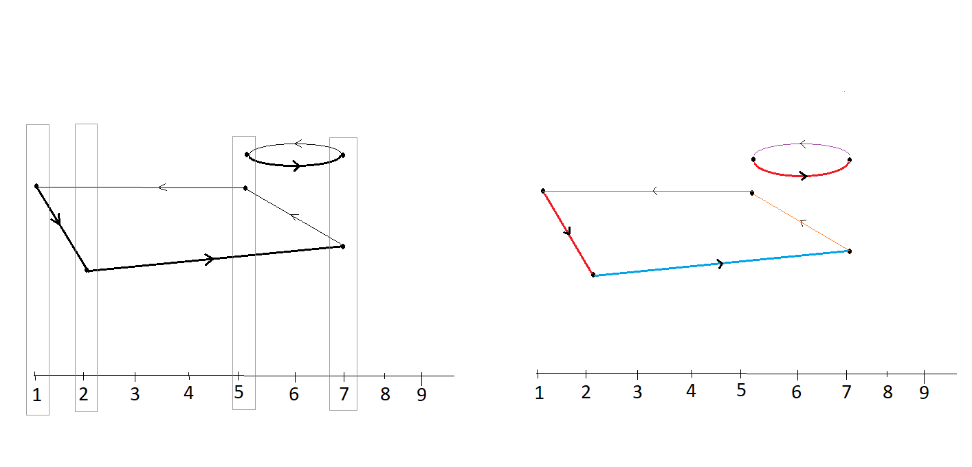
We now discuss the coloring of such a directed graph given budget constraints. For we call (resp. ) a positively oriented edge (resp. negatively oriented). We will use distinct sets of colors for each orientation.
Definition.
Consider a directed graph satisfying the -condition. Choose ’positive’ colors and ’negative’ colors, and partition the set of positive colors so that of them have budget . Similarly, partition the set of negative colors so that of them have budget (If a color has budget it means that the total weight of edges colored with it have to add up to ).
A coloring of is non-overlapping if implies that the edges and have distinct colors (similarly the negatively oriented edges and should have distinct colors)
Let’s give an explicit example of the budget rule based on figure 1. If, for example, we have for negatively oriented edges. It implies that we have a total of 3 distinct colors, where 2 of them each have a budget constraint of and the other one has a budget constraint of . Also, note that an edge will allocate from the coloring budget based on the weight assigned to it.
Theorem 6.3.
Fix with and . Let denote the set of all possible directed graphs satisfying -condition and let be the number of non-overlapping colorings of according to the color budget given by . Then
Furthermore, the set of possible graphs satisfying -condition can be constructed as in Lemma 7.
Proof.
Here is how one translates the index families in theorem 6.1 into a graph with integer vertices. The indices defined by and (resp. and ) identify the positively oriented (resp. negatively oriented) edges in the graph, in the following way. For any pair and we define a positively oriented edge from the vertex to . The rule is similar for negatively oriented edges. ∎
We have the following dictionary for various combinatorial quantities, consistent with previous sections:
- •
: number of nodes in .
- •
: number of edges in .
- •
: in-going and out-going degree of node .
- •
; total color budget used to color positively oriented edges.
- •
: total color budget used to color negatively oriented edges.
- •
: number of distinct colors used to color positively oriented edges.
- •
: number of distinct colors used to color negatively oriented edges.
- •
: number of colors with budget for positively oriented edges.
- •
: number of colors with budget for negatively oriented edges.
References
- [1] K. Astala, P. Jones, A. Kupiainen, and Saksman, Random curves by conformal welding, Acta Math. 207, No. 2 (2011) 203-254.
- [2] N. Berestycki, An elementary approach to Gaussian multiplicative chaos, Electronic Communications in Probability, 22 (2017) Paper No. 27.
- [3] P. Billingsley, Convergence of Probability Measures, John Wiley and Sons (1968)
- [4] A. Caine and D. Pickrell, Loops in noncompact groups of Hermitian symmetric type and factorization. J. Gen. Lie Theory Appl., 9, no. 2, Art. ID 1000233 (2015)
- [5] R. Chhaibi, J. Najnudel, On the circle, for , , arXiv:1904.00578
- [6] J.P. Kahane, Some Random Series of Functions, 2nd edition, Cambridge Univ. Press (1993)
- [7] S. Lang, , Addison-Wesley Publishing Co., Reading, Massachusetts (1975)
- [8] M. Latifi and D. Pickrell, Exponential of the Trace of the Free Field and Verblunsky Coefficients, II: Combinatorics, (to appear on the ArXiv)
- [9] S. Kerov, G. Olshansky and A. Vershik, Harmonic analysis on the infinite symmetric group, Inv. Math. 158, No. 3 (2004) 551-642.
- [10] I. Segal, Ergodic subgroups of the orthogonal group on a real Hilbert space, Annals of Mathematics, Vol. 66, no. 2 (1957) 297-303.
- [11] B. Simon, The Euclidean (Quantum) Field Theory, Princeton Series in Physics, Princeton Univ. Press (1974).
- [12] B. Simon, Orthogonal Polynomials on the Unit Circle, Part I Classical Theory, AMS Colloquium Series, Amer. Math. Soc., Providence, RI (2005)
- [13] B. Simon, OPUC on one foot, Bull. Amer.Math. Soc., Vol. 42, No 4 (2005) 431-460.
- [14] M. Sodin, Zeroes of Gaussian analytic functions, arXiv:math.CV/0410343