跳到论文正文
W Papers独立论文阅读器 arXiv:2002.06453 论文正文 计算阅读时间 · 0%
引用这篇论文根据当前论文元数据生成,正式投稿前建议核对。


License: arXiv.org perpetual non-exclusive license
arXiv:2002.06453v1 [eess.SP] 15 Feb 2020

Channel Estimation for RIS-Aided mmWave MIMO Channels Thanks: This work is supported by Horizon 2020, European Union’s Framework Programme for Research and Innovation, under grant agreement no. 871464 (ARIADNE). This work is also partially supported by the Academy of Finland 6Genesis Flagship (grant 318927) and Swedish Research Council (grant no. 2018-03701). The work of M. Leinonen has been financially supported in part by Infotech Oulu and the Academy of Finland (grant 319485 and 323698).

Jiguang He Affiliation: Centre for Wireless Communications, FI-90014, University of Oulu, Finland    Markus Leinonen Affiliation: Centre for Wireless Communications, FI-90014, University of Oulu, Finland    Henk Wymeersch Affiliation: Department of Electrical Engineering, Chalmers University of Technology, Gothenburg, Sweden    Markku Juntti Affiliation: Centre for Wireless Communications, FI-90014, University of Oulu, Finland
Abstract

A reconfigurable intelligent surface (RIS) can shape the radio propagation by passively changing the directions of impinging electromagnetic waves. The optimal control of the RIS requires perfect channel state information (CSI) of all the links connecting the base station (BS) and the mobile station (MS) via the RIS. Thereby the channel (parameter) estimation at the BS/MS and the related message feedback mechanism are needed. In this paper, we adopt a two-stage channel estimation scheme for the RIS-aided millimeter wave (mmWave) MIMO channels using an iterative reweighted method to sequentially estimate the channel parameters. We evaluate the average spectrum efficiency (SE) and the RIS beamforming gain of the proposed scheme and demonstrate that it achieves high-resolution estimation with the average SE comparable to that with perfect CSI.

Index Terms: 
Channel estimation, compressive sensing, millimeter wave MIMO, reconfigurable intelligent surface.

I Introduction

Large unused spectrum is available in the millimeter wave (mmWave) bands. In order to compensate for the high free space path loss, large antenna arrays are needed both at the transmitters and receivers [1, 2, 3]. This makes the channel estimation (CE) more difficult than that in conventional sub-6 GHz multiple-input multiple-output (MIMO) systems having less transmit and receive antennas. The mmWave MIMO channel is inherently sparse due to the limited number of distinguishable paths in the angular domain. Thus, compressive sensing (CS) techniques, which take advantage of the sparsity, have been widely applied in the channel (parameter) estimation of mmWave MIMO channels, e.g., in [4, 5].

In order to further improve the spectrum efficiency (SE) and to guarantee a wide communication coverage, the concept of a reconfigurable intelligent surface (RIS) has been recently proposed to smartly shape the propagation of electromagnetic waves [6, 7, 8, 9]. The RIS also has great potential to offer higher accuracy of positioning and localization, both for indoor and outdoor, compared to the system without RISs [9, 10]. The RIS can be made of an array of phase shifters, which can passively steer the beams towards the dedicated user(s) by controlling the phase of each RIS unit. This RIS architecture is called the discrete RIS. Another type of RIS is the contiguous RIS which can be seen as an active transceiver [6].

CE for RIS-aided MIMO systems has been recently studied in [11, 12]. In [11], CE is performed using CS and deep learning methods in a setup with a few active elements at the RIS. In [12], sparse matrix factorization and matrix completion are exploited in a sequential manner to perform iterative CE. In this work, full advantage of the RIS is not achieved due to the on/off state applied to the RIS elements. Instead of estimating the MIMO channels, a multi-level codebook based scheme was leveraged to design the phase control matrix at the RIS and the combining vector at the MS jointly [13].

In the paper, we study the CE problem of the passive RIS-aided mmWave MIMO system. We divide the CE problem into two subproblems and apply an iterative reweighted method to find the estimates of the channel parameters sequentially. In the first stage, we estimate the angle of departure (AoD) for the BS-RIS link, the angle of arrival (AoA) of the RIS-MS link, and the corresponding effective propagation path gains. In the second stage, we estimate the product of the propagation path gains of the BS-RIS link and the RIS-MS link and the difference of directional sine of the AoA of the BS-RIS and the AoD of RIS-MS link. Besides evaluating the mean square error (MSE) of the estimated channel parameters, we design the RIS phase control matrix, the BS beamforming (BF) vector, and the MS combining vector based on the estimates and evaluate the average SE and RIS BF gain. The performance of the proposed scheme is compared to that of an orthogonal matching pursuit (OMP) approach. Simulation results demonstrate that average SE achieved by the proposed method approaches that with perfect channel state information (CSI), even in the low signal-to-noise ratio (SNR) regime with limited training overhead.

Notation: A bold lowercase letter 𝐚{\mathbf{a}} denotes the column vector, a bold capital letter 𝐀{\mathbf{A}} denotes the matrix, (⋅)𝖧(\cdot)^{\mathsf{H}}, (⋅)𝖳(\cdot)^{\mathsf{T}}, and (⋅)∗(\cdot)^{*} denote the Hermitian transpose, transpose, and conjugate, respectively, diag⁡(𝐚)\mathrm{diag}({\mathbf{a}}) denotes a square diagonal matrix with entries of 𝐚{\mathbf{a}} on its diagonal, 𝐚∘𝐛{\mathbf{a}}\circ{\mathbf{b}} denotes the Hadamard product of 𝐚{\mathbf{a}} and 𝐛{\mathbf{b}}, [𝐚]i[{\mathbf{a}}]_{i} denotes the iith element of vector 𝐚{\mathbf{a}}, [𝐀]i​j[{\mathbf{A}}]_{ij} denotes the (i,j)(i,j)th element of 𝐀{\mathbf{A}}, and ∥⋅∥F\|\cdot\|_{\mathrm{F}} is the Frobenius norm.

II Channel Model
Refer to caption
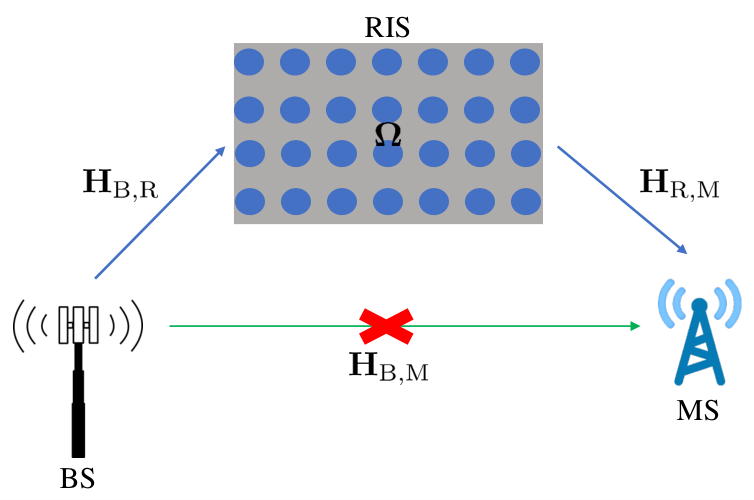
Fig. 1: The considered RIS-aided mmWave MIMO system with one BS, one MS, and one RIS.

We consider the RIS-aided mmWave MIMO system that comprises one multi-antenna BS, one multi-antenna MS, and one multi-element RIS, as depicted in Fig. 1. The numbers of antenna elements are defined as NBSN_{\text{BS}}, NMSN_{\text{MS}}, and NRISN_{\text{RIS}}, respectively. The antenna array is assumed to be an uniform linear array (ULA); an extension to an uniform planar array (UPA) is feasible. We assume that the direct link between the BS and the MS are obstructed, which renders the potential usage of a RIS for maintaining the connectivity.

We assume geometric channel model. The channel between the BS and the RIS 𝐇B,R∈ℂNRIS×NBS{\mathbf{H}}_{\text{B,R}}\in\mathbb{C}^{N_{\text{RIS}}\times N_{\text{BS}}} is

𝐇B,R=∑l=0LB,RρB,R,l​𝜶​(ϕB,R,l)​𝜶𝖧​(θB,R,l),{\mathbf{H}}_{\text{B,R}}=\sum\limits_{l=0}^{L_{\text{B,R}}}\rho_{\text{B,R},l}\boldsymbol{\alpha}(\phi_{\text{B,R},l})\boldsymbol{\alpha}^{\mathsf{H}}(\theta_{\text{B,R},l}), (1)

where θB,R,l\theta_{\text{B,R},l} and ϕB,R,l\phi_{\text{B,R},l} denote the llth AoD and AoA of the BS-RIS link, respectively, LB,RL_{\text{B,R}} denotes the number of resolvable paths, which is usually on the order of 3–5 in mmWave bands [14], and ρB,R,l\rho_{\text{B,R},l} denotes the iith propagation path gain. Index l=0{l=0} refers to the line-of-sight (LoS) path, and l=1,⋯,LB,Rl=1,\cdots,L_{\text{B,R}} refer to the non-line-of-sight (NLoS) paths, e.g., single-bounce or multi-bounce reflection paths. Usually, |ρB,R,0|2≫|ρB,R,l|2|\rho_{\text{B,R},0}|^{2}\gg|\rho_{\text{B,R},l}|^{2} for l=1,⋯,LB,Rl=1,\cdots,L_{\text{B,R}}, and the difference is easily more than 20 dB [15]. Finally, 𝜶⁡(θB,R,l)∈ℂNBS×1{\boldsymbol{\alpha}(\theta_{\text{B,R},l})\in\mathbb{C}^{N_{\text{BS}}\times 1}} and 𝜶⁡(ϕB,R,l)∈ℂNRIS×1{\boldsymbol{\alpha}(\phi_{\text{B,R},l})\in\mathbb{C}^{N_{\text{RIS}}\times 1}} are the array response vectors with [𝜶⁡(θB,R,l)]k=exp⁡(j​2​π​dλ​(k−1)​sin⁡(θB,R,l))[\boldsymbol{\alpha}(\theta_{\text{B,R},l})]_{k}=\exp\big(j2\pi\frac{d}{\lambda}(k-1)\sin(\theta_{\text{B,R},l})\big) for k=1,⋯,NBSk=1,\cdots,N_{\text{BS}} and [𝜶⁡(ϕB,R,l)]k=exp⁡(j​2​π​dλ​(k−1)​sin⁡(ϕB,R,l))[\boldsymbol{\alpha}(\phi_{\text{B,R},l})]_{k}=\exp\big(j2\pi\frac{d}{\lambda}(k-1)\sin(\phi_{\text{B,R},l})\big) for k=1,⋯,NRISk=1,\cdots,N_{\text{RIS}}, where dd is the antenna element spacing, λ\lambda is the wavelength of the carrier frequency, and j​=△​−1j\overset{\triangle}{=}\sqrt{-1}.

Similarly, the channel between the RIS and the MS, denoted as 𝐇R,M∈ℂNMS×NRIS{\mathbf{H}}_{\text{R,M}}\in\mathbb{C}^{N_{\text{MS}}\times N_{\text{RIS}}}, is

𝐇R,M=∑l=0LR,MρR,M,l​𝜶​(ϕR,M,l)​𝜶𝖧​(θR,M,l).{\mathbf{H}}_{\text{R,M}}=\sum\limits_{l=0}^{L_{\text{R,M}}}\rho_{\text{R,M},l}\boldsymbol{\alpha}(\phi_{\text{R,M},l})\boldsymbol{\alpha}^{\mathsf{H}}(\theta_{\text{R,M},l}). (2)

Using (1) and (2), the composite channel 𝐇∈ℂNMS×NBS{{\mathbf{H}}\in\mathbb{C}^{N_{\text{MS}}\times N_{\text{BS}}}} between the BS and MS becomes

𝐇=𝐇R,M​𝛀​𝐇B,R,{\mathbf{H}}={\mathbf{H}}_{\text{R,M}}\boldsymbol{\Omega}{\mathbf{H}}_{\text{B,R}}, (3)

where 𝛀∈ℂNRIS×NRIS\boldsymbol{\Omega}\in\mathbb{C}^{N_{\text{RIS}}\times N_{\text{RIS}}} is the phase control matrix at the RIS. The matrix 𝛀\boldsymbol{\Omega} is a diagonal matrix with unit-modulus elements on the diagonal, i.e., [𝛀]k​k=exp⁡(j​ω)[\boldsymbol{\Omega}]_{kk}=\exp(j\omega) with ω∈ℝ\omega\in\mathbb{R}. In practice, the reflection may not be perfect so that reflection coefficient a∈[0, 1]a\in[0,\;1] as [𝛀]k​k=a​exp⁡(j​ω)[\boldsymbol{\Omega}]_{kk}=a\exp(j\omega) describes the amplitude scaling and power loss [16]; however, we assume that a=1a=1.

Since the LoS path is typically much stronger than the NLoS paths according to the field measurements in [15], we ignore the NLoS paths in the BS-RIS and RIS-MS links, and approximate the composite channel in (3) as

𝐇\displaystyle{\mathbf{H}} ≈𝜶⁡(ϕR,M,0)​ρR,M,0​𝜶𝖧​(θR,M,0)​𝛀​𝜶​(ϕB,R,0)​ρB,R,0​𝜶𝖧​(θB,R,0)\displaystyle\approx\boldsymbol{\alpha}(\phi_{\text{R,M},0})\rho_{\text{R,M},0}\boldsymbol{\alpha}^{\mathsf{H}}(\theta_{\text{R,M},0})\boldsymbol{\Omega}\boldsymbol{\alpha}(\phi_{\text{B,R},0})\rho_{\text{B,R},0}\boldsymbol{\alpha}^{\mathsf{H}}(\theta_{\text{B,R},0})
=g​𝜶​(ϕR,M,0)​𝜶𝖧​(θB,R,0),\displaystyle=g\boldsymbol{\alpha}(\phi_{\text{R,M},0})\boldsymbol{\alpha}^{\mathsf{H}}(\theta_{\text{B,R},0}), (4)

where g∈ℂg\in\mathbb{C} is the effective propagation path gain, defined as

g=ρB,R,0​ρR,M,0​𝜶𝖧​(θR,M,0)​𝛀​𝜶​(ϕB,R,0).g=\rho_{\text{B,R},0}\rho_{\text{R,M},0}\boldsymbol{\alpha}^{\mathsf{H}}(\theta_{\text{R,M},0})\boldsymbol{\Omega}\boldsymbol{\alpha}(\phi_{\text{B,R},0}). (5)

According to (4) and (5), the composite channel is virtually a point-to-point MIMO channel with one path via the RIS. The rank of 𝐇{\mathbf{H}} is 1≪{NBS,NMS}1\ll\{N_{\text{BS}},N_{\text{MS}}\}. Thus, the channel encompasses a sparse structure in the angular domain – characteristic to an mmWave channel – which can efficiently be leveraged by CS.

III Sounding Procedure

We assume that the channels suffer from block fading. For the sounding process, one coherence time interval is divided into two subintervals, the first one for CE and the second for data transmission (DT), as depicted in Fig. 2. The CE subinterval is further divided into multiple blocks.

Refer to caption
Fig. 2: The sounding and CE procedure. Each CE subinterval contains multiple blocks where 𝛀t\boldsymbol{\Omega}_{t} varies over the blocks.

In each block t=1,⋯,T{t=1,\cdots,T}, the BS sends a (random) training matrix 𝐗t∈ℂNBS×NX{\mathbf{X}}_{t}\in\mathbb{C}^{N_{\text{BS}}\times N_{X}} which, after reflected from the RIS having a (random) phase control matrix 𝛀t\boldsymbol{\Omega}_{t}, is received at the MS through a (random) combining matrix 𝐖t∈ℂNMS×NW{\mathbf{W}}_{t}\in\mathbb{C}^{N_{\text{MS}}\times N_{W}}. Thus, the received signal at the MS is given as

𝐘t=𝐖t𝖧𝐇(𝛀t)𝐗t+𝐖t𝖧𝐍t,t=1,⋯,T,{\mathbf{Y}}_{t}={\mathbf{W}}_{t}^{\mathsf{H}}{\mathbf{H}}(\boldsymbol{\Omega}_{t}){\mathbf{X}}_{t}+{\mathbf{W}}_{t}^{\mathsf{H}}{\mathbf{N}}_{t},\;t=1,\cdots,T, (6)

where we write 𝐇{\mathbf{H}} explicitly as a function of 𝛀t\boldsymbol{\Omega}_{t}. Further, let

gt=ρR,M,0​ρB,R,0​𝜶𝖧​(θR,M,0)​𝛀t​𝜶​(ϕB,R,0).g_{t}=\rho_{\text{R,M},0}\rho_{\text{B,R},0}\boldsymbol{\alpha}^{\mathsf{H}}(\theta_{\text{R,M},0})\boldsymbol{\Omega}_{t}\boldsymbol{\alpha}(\phi_{\text{B,R},0}). (7)

The following assumptions are made for the CE subinterval:

  • •

    All the channel parameters stay unchanged within the coherence time.

  • •

    𝛀t\boldsymbol{\Omega}_{t} is varying with block index tt, and it is constructed with randomly generated phases ω∈[−π​π]\omega\in[-\pi\;\pi].

  • •

    𝐖t{\mathbf{W}}_{t} and 𝐗t{\mathbf{X}}_{t} are varying with block index tt.

IV Two-Stage CE Approach

We consider a two-stage approach to simplify the CE problem. The solution process is summarized in Algorithm 1. The details of the algorithm will be provided in the sequel.

Algorithm 1 Two-stage CE Approach
1: ⊳\triangleright First stage
2: Received signals 𝐘1,…,𝐘T{\mathbf{Y}}_{1},\dots,{\mathbf{Y}}_{T}, combining matrices 𝐖1,…,𝐖T{\mathbf{W}}_{1},\dots,{\mathbf{W}}_{T}, training matrices 𝐗1,…,𝐗T{\mathbf{X}}_{1},\dots,{\mathbf{X}}_{T}, phase control matrices 𝛀1,…,𝛀T\boldsymbol{\Omega}_{1},\dots,\boldsymbol{\Omega}_{T}, and threshold value τth\tau_{\text{th}}.
3: θ^,ϕ^\hat{\theta},\hat{\phi}, and 𝐠^\hat{{\mathbf{g}}}.
4: Initial θ(i)\theta^{(i)} and ϕ(i)\phi^{(i)} for i=0i=0 by the SVD based approach.
5: repeat
6:   Compute g^t(i+1)\hat{g}_{t}^{(i+1)} by (10).
7:   Construct the objective function S~​(𝐠^(i+1),θ,ϕ)\tilde{S}(\hat{{\mathbf{g}}}^{(i+1)},\theta,\phi) by (IV-A).
8:   Use gradient descent to minimize S~​(𝐠^(i+1),θ,ϕ)\tilde{S}(\hat{{\mathbf{g}}}^{(i+1)},\theta,\phi).
9: until The maximum number of iterations reached or ‖𝐠^(i+1)−𝐠^(i)‖2<τth\|\hat{{\mathbf{g}}}^{(i+1)}-\hat{{\mathbf{g}}}^{(i)}\|_{2}<\tau_{\text{th}}.
10: ⊳\triangleright Second stage
11: 𝐠^\hat{{\mathbf{g}}} and threshold value τ~th\tilde{\tau}_{\text{th}}.
12: q^\hat{q} and θ~^\hat{\tilde{\theta}}.
13: Initial θ~(i)\tilde{\theta}^{(i)} for i=0i=0.
14: repeat
15:   Compute q^(i+1)\hat{q}^{(i+1)}.
16:   Construct the objective function J~​(q^(i+1),θ~)\tilde{J}(\hat{q}^{(i+1)},\tilde{\theta}) by (17).
17:   Use gradient descent to minimize J~​(q^(i+1),θ~)\tilde{J}(\hat{q}^{(i+1)},\tilde{\theta}).
18: until The maximum number of iterations reached or |q^(i+1)−q^(i)|<τ~th|\hat{q}^{(i+1)}-\hat{q}^{(i)}|<\tilde{\tau}_{\text{th}}.

IV-A First Stage

In the first stage, we estimate the AoD of the BS-RIS link θB,R,0\theta_{\text{B,R},0} in (4), the AoA of the RIS-MS link ϕR,M,0\phi_{\text{R,M},0} in (4), and the effective propagation path gain of the reflection link gtg_{t} in (7) based on the received signals {𝐘t}t=1T\{{\mathbf{Y}}_{t}\}_{t=1}^{T}. Typically, the CS methods like OMP have been proposed for CE. One drawback is that they only can recover angular estimates that lie on a pre-defined grid of discrete angles. This “on-the-grid” problem, which inevitably deteriorates the CE performance, can be counteracted by the iterative reweighted method [8], used herein as well.

Using the iterative reweighted method, the CE problem in the first stage is formulated as

min𝐠,θ,ϕ​S​(𝐠,θ,ϕ)=∑t=1Tln⁡(|gt|2+ϵ)+ξ​‖𝐘t−𝐖t𝖧​𝐇​(𝛀t)​𝐗t‖F2,\underset{{\mathbf{g}},\theta,\phi}{\min}S({\mathbf{g}},\theta,\phi)=\sum_{t=1}^{T}\ln(|g_{t}|^{2}+\epsilon)+\xi\|{\mathbf{Y}}_{t}-{\mathbf{W}}_{t}^{\mathsf{H}}{\mathbf{H}}(\boldsymbol{\Omega}_{t}){\mathbf{X}}_{t}\|^{2}_{\mathrm{F}}, (8)

where 𝐠=[g1,⋯,gT]𝖳{\mathbf{g}}=[g_{1},\cdots,g_{T}]^{\mathsf{T}}, parameter ϵ>0\epsilon>0 ensures that the argument of ln⁡(⋅)\mathrm{ln}(\cdot) is positive, ξ>0\xi>0 controls the tradeoff between the sparsity of 𝐠{\mathbf{g}} and data fitting. Here, we replaced ϕR,M,0\phi_{\text{R,M},0} and θB,R,0\theta_{\text{B,R},0} with ϕ\phi and θ\theta to simplify the notations. The sparsity-inducing ln⁡(⋅)\mathrm{ln}(\cdot) term accounts for the fact that due to the random generation of 𝛀t\boldsymbol{\Omega}_{t}, t=1,⋯,Tt=1,\cdots,T, some elements in 𝐠{\mathbf{g}} may be much smaller than others.

The problem in (8) can be further formulated as [17]

min𝐠,θ,ϕ⁡S~​(𝐠,θ,ϕ)=𝐠𝖧​𝐆(i)​𝐠+ξ​∑t=1T‖𝐘t−𝐖t𝖧​𝐇​(𝛀t)​𝐗t‖F2,\min_{{\mathbf{g}},\theta,\phi}\tilde{S}({\mathbf{g}},\theta,\phi)={\mathbf{g}}^{\mathsf{H}}{\mathbf{G}}^{(i)}{\mathbf{g}}+\xi\sum_{t=1}^{T}\|{\mathbf{Y}}_{t}-{\mathbf{W}}_{t}^{\mathsf{H}}{\mathbf{H}}(\boldsymbol{\Omega}_{t}){\mathbf{X}}_{t}\|^{2}_{\mathrm{F}}, (9)

where

𝐆(i)=diag⁡([1|g^1(i)|2+ϵ,⋯,1|g^T(i)|2+ϵ]𝖳){{\mathbf{G}}^{(i)}=\mathrm{diag}\Big(\big[\frac{1}{|\hat{g}^{(i)}_{1}|^{2}+\epsilon},\cdots,\frac{1}{|\hat{g}^{(i)}_{T}|^{2}+\epsilon}\big]^{\mathsf{T}}\Big)}

and g^t(i)\hat{g}^{(i)}_{t} is an estimate of gtg_{t} at the iith iteration. Setting the first-order partial derivative of S~​(𝐠,θ,ϕ)\tilde{S}({\mathbf{g}},\theta,\phi) in (9) with respect to gtg_{t} to zero yields

g^t(i+1)=(1ξ⁡(|g^t(i)|2+ϵ)+‖𝐀t​𝐗t‖F2)−1​∑k=1NX𝐱t,k𝖧​𝐀t𝖧​𝐲t,k,\hat{g}_{t}^{(i+1)}=\Bigg(\frac{1}{\xi(|\hat{g}^{(i)}_{t}|^{2}+\epsilon)}+\|{\mathbf{A}}_{t}{\mathbf{X}}_{t}\|_{\mathrm{F}}^{2}\Bigg)^{-1}\sum_{k=1}^{N_{X}}{\mathbf{x}}_{t,k}^{\mathsf{H}}{\mathbf{A}}_{t}^{\mathsf{H}}{\mathbf{y}}_{t,k}, (10)

where 𝐱t,k{\mathbf{x}}_{t,k} and 𝐲t,k{\mathbf{y}}_{t,k} is the kkth column of 𝐗t{\mathbf{X}}_{t} and 𝐘t{\mathbf{Y}}_{t}, respectively, and 𝐀t=𝐖t𝖧​𝜶​(ϕ)​𝜶𝖧​(θ){\mathbf{A}}_{t}={\mathbf{W}}_{t}^{\mathsf{H}}\boldsymbol{\alpha}(\phi)\boldsymbol{\alpha}^{\mathsf{H}}(\theta). Thus, for given 𝐠^(i+1)=[g^1(i+1),⋯,g^T(i+1)]𝖳\hat{{\mathbf{g}}}^{(i+1)}=[\hat{g}_{1}^{(i+1)},\cdots,\hat{g}_{T}^{(i+1)}]^{\mathsf{T}}, (9) can be written as

S~​(𝐠^(i+1),θ,ϕ)=1ξ​∑t=1Tβt2​zt∗​zt​1|g^t(i)|2+ϵ+∑t=1T∑k=1NX𝐲t,k𝖧​𝐲t,k\displaystyle\tilde{S}(\hat{{\mathbf{g}}}^{(i+1)},\theta,\phi)=\frac{1}{\xi}\sum_{t=1}^{T}\beta_{t}^{2}z_{t}^{*}z_{t}\frac{1}{|\hat{g}^{(i)}_{t}|^{2}+\epsilon}+\sum_{t=1}^{T}\sum_{k=1}^{N_{X}}{\mathbf{y}}_{t,k}^{\mathsf{H}}{\mathbf{y}}_{t,k}
+∑t=1T{−g^t(i+1)zt∗−(g^t(i+1))∗zt+|g^t(i+1)|2∥𝐀t𝐗t∥F2}\displaystyle+\sum_{t=1}^{T}\left\{-\hat{g}_{t}^{(i+1)}z_{t}^{*}-\left(\hat{g}_{t}^{(i+1)}\right)^{*}z_{t}+|\hat{g}_{t}^{(i+1)}|^{2}\|{\mathbf{A}}_{t}{\mathbf{X}}_{t}\|_{\mathrm{F}}^{2}\right\}
=∑t=1T(−βt​zt∗​zt+∑k=1NX𝐲t,k𝖧​𝐲t,k),\displaystyle=\sum_{t=1}^{T}\left(-\beta_{t}z_{t}^{*}z_{t}+\sum_{k=1}^{N_{X}}{\mathbf{y}}_{t,k}^{\mathsf{H}}{\mathbf{y}}_{t,k}\right), (11)

where we defined the quantities zt=∑k=1NX𝐱t,k𝖧​𝐀t𝖧​𝐲t,k{z_{t}=\sum\limits_{k=1}^{N_{X}}{\mathbf{x}}_{t,k}^{\mathsf{H}}{\mathbf{A}}_{t}^{\mathsf{H}}{\mathbf{y}}_{t,k}} and βt=(1ξ⁡(|g^t(i)|2+ϵ)+‖𝐀t​𝐗t‖F2)−1{\beta_{t}=\Big(\frac{1}{\xi(|\hat{g}^{(i)}_{t}|^{2}+\epsilon)}+\|{\mathbf{A}}_{t}{\mathbf{X}}_{t}\|_{\mathrm{F}}^{2}\Big)^{-1}}.

The above equations give rise to an iterative algorithm aiming at minimizing the objective function in (IV-A). To this end, we propose Algorithm 1 where at each iteration ii, we use a gradient descent algorithm to find estimates for the angles θ\theta and ϕ\phi for a given 𝐠^(i+1)\hat{{\mathbf{g}}}^{(i+1)} in (10). The calculation of the required first-order partial derivatives associated with θ\theta and ϕ\phi is presented in Appendix -A. The initial values for θ\theta and ϕ\phi, defined as θ(0)\theta^{(0)} and ϕ(0)\phi^{(0)}, can be determined by the singular value decomposition (SVD) based approach [8]. After a certain stopping criterion is met, we proceed to the second stage.

IV-B Second Stage

In the second stage, we estimate the remaining channel parameters based on the final estimate of 𝐠{\mathbf{g}} obtained in the first stage, denoted as 𝐠^=[g^1,⋯,g^T]𝖳\hat{{\mathbf{g}}}=[\hat{g}_{1},\cdots,\hat{g}_{T}]^{\mathsf{T}}. Obtaining a separate estimate of the AoA for the BS-RIS link ϕB,R,0\phi_{\text{B,R},0} and the AoD for the RIS-MS link θR,M,0\theta_{\text{R,M},0} seems infeasible; the same holds for the propagation path gains in the BS-RIS and RIS-MS links ρR,M,0\rho_{\text{R,M},0} and ρB,R,0\rho_{\text{B,R},0}. Thus, instead, we will estimate the product of the propagation path gains ρR,M,0​ρB,R,0\rho_{\text{R,M},0}\rho_{\text{B,R},0} and the difference of directional sine, defined as θdiff=sin⁡(ϕR,M,0)−sin⁡(θB,R,0)\theta_{\text{diff}}=\sin(\phi_{\text{R,M},0})-\sin(\theta_{\text{B,R},0}).

According to (7), we rewrite gtg_{t} as

gt=ρR,M,0​ρB,R,0​𝝎t𝖳​(𝜶∗​(θR,M,0)∘𝜶⁡(ϕB,R,0)),g_{t}=\rho_{\text{R,M},0}\rho_{\text{B,R},0}\boldsymbol{\omega}_{t}^{\mathsf{T}}\big(\boldsymbol{\alpha}^{*}(\theta_{\text{R,M},0})\circ\boldsymbol{\alpha}(\phi_{\text{B,R},0})\big), (12)

where 𝝎t∈ℂNRIS×1{\boldsymbol{\omega}_{t}\in\mathbb{C}^{N_{\text{RIS}}\times{1}}} is the vector of phase control matrix values as 𝛀t=diag⁡(𝝎t){\boldsymbol{\Omega}_{t}=\mathrm{diag}(\boldsymbol{\omega}_{t})}. By stacking the TT different 𝝎t\boldsymbol{\omega}_{t}’s row-wise as 𝛀~=[𝝎1,⋯,𝝎T]𝖳\tilde{\boldsymbol{\Omega}}=[\boldsymbol{\omega}_{1},\cdots,\boldsymbol{\omega}_{T}]^{\mathsf{T}} and introducing q=ρR,M,0​ρB,R,0q=\rho_{\text{R,M},0}\rho_{\text{B,R},0} and θ~=asin⁡(θdiff)\tilde{\theta}=\mathrm{asin}(\theta_{\text{diff}}), we have

𝐠=𝛀~​ρR,M,0​ρB,R,0​(𝜶∗​(θR,M,0)∘𝜶⁡(ϕB,R,0))=q​𝛀~​𝜶​(θ~).{\mathbf{g}}\!=\tilde{\boldsymbol{\Omega}}\rho_{\text{R,M},0}\rho_{\text{B,R},0}\big(\boldsymbol{\alpha}^{*}(\theta_{\text{R,M},0})\!\circ\!\boldsymbol{\alpha}(\phi_{\text{B,R},0})\big)\!=q\tilde{\boldsymbol{\Omega}}\boldsymbol{\alpha}(\tilde{\theta}). (13)

Recall that the the angular sparsity is one. Regarding this fact, we aim at finding the sparsest representation while minimizing the MSE of the data fitting, which fits in the problem of line spectral estimation [17]. Further, we assume that

𝐠^=𝐠+𝐧=q​𝛀~​𝜶​(θ~)+𝐧,\hat{{\mathbf{g}}}={\mathbf{g}}+{\mathbf{n}}=q\tilde{\boldsymbol{\Omega}}\boldsymbol{\alpha}(\tilde{\theta})+{\mathbf{n}}, (14)

where the estimation error 𝐧{\mathbf{n}} from the first stage is modelled as additive Gaussian noise, independent of qq and θ~\tilde{\theta}. Thus, the objective function of the second stage estimation problem is formulated as

min⁡J⁡(q,θ~)=ln⁡(|q|2+ϵ)+μ​‖𝐠^−𝛀~​𝐡‖22,\min J(q,\tilde{\theta})=\ln(|q|^{2}+\epsilon)+\mu\|\hat{{\mathbf{g}}}-\tilde{\boldsymbol{\Omega}}{\mathbf{h}}\|_{2}^{2}, (15)

where 𝐡=q​𝜶​(θ~){\mathbf{h}}=q\boldsymbol{\alpha}(\tilde{\theta}) and μ\mu is a parameter that controls the tradeoff between the sparsity and data fitting. The objective function can be further reformulated as

min⁡J~​(q,θ~)=q​q∗|q^(i)|2+ϵ+μ​‖𝐠^−𝛀~​𝐡‖22.\min\tilde{J}(q,\tilde{\theta})=\frac{qq^{*}}{|\hat{q}^{(i)}|^{2}+\epsilon}+\mu\|\hat{{\mathbf{g}}}-\tilde{\boldsymbol{\Omega}}{\mathbf{h}}\|_{2}^{2}. (16)

We also follow the iterative reweighted method to find the high-resolution estimate of θ~\tilde{\theta}. At the beginning, we find an initial estimate of θ~\tilde{\theta} on the grid as θ~(0)=arg⁡maxθ~∈Υ​|𝐠^𝖧​𝛀~​𝐡|,\tilde{\theta}^{(0)}=\arg\max_{\tilde{\theta}\in\Upsilon}|\hat{{\mathbf{g}}}^{\mathsf{H}}\tilde{\boldsymbol{\Omega}}{\mathbf{h}}|, where Υ\Upsilon is a quantized set of angles within [−π​π][-\pi\;\pi]. Setting the derivative of the objective function J~​(q,θ~)\tilde{J}(q,\tilde{\theta}) in (16) with respect to qq to zero yields q^(i+1)=γ​𝜶​(θ~)𝖧​𝛀~𝖧​𝐠^\hat{q}^{(i+1)}=\gamma\boldsymbol{\alpha}(\tilde{\theta})^{\mathsf{H}}\tilde{\boldsymbol{\Omega}}^{\mathsf{H}}\hat{{\mathbf{g}}}, where γ=(1/(μ⁡(|q^(i)|2+ϵ))+𝜶​(θ~)𝖧​𝛀~𝖧​𝛀~​𝜶​(θ~))−1\gamma=\big({1}/({\mu(|\hat{q}^{(i)}|^{2}+\epsilon)})+\boldsymbol{\alpha}(\tilde{\theta})^{\mathsf{H}}\tilde{\boldsymbol{\Omega}}^{\mathsf{H}}\tilde{\boldsymbol{\Omega}}\boldsymbol{\alpha}(\tilde{\theta})\big)^{-1}. For fixed q^(i+1)\hat{q}^{(i+1)}, the objective function can be further written as

J~​(q^(i+1),θ~)=−γ​τ+𝐠^𝖧​𝐠^.\tilde{J}(\hat{q}^{(i+1)},\tilde{\theta})=-\gamma\tau+\hat{{\mathbf{g}}}^{\mathsf{H}}\hat{{\mathbf{g}}}. (17)

where τ=𝜶​(θ~)𝖧​𝛀~𝖧​𝐠^​𝐠^𝖧​𝛀~​𝜶​(θ~)\tau=\boldsymbol{\alpha}(\tilde{\theta})^{\mathsf{H}}\tilde{\boldsymbol{\Omega}}^{\mathsf{H}}\hat{{\mathbf{g}}}\hat{{\mathbf{g}}}^{\mathsf{H}}\tilde{\boldsymbol{\Omega}}\boldsymbol{\alpha}(\tilde{\theta}). Based on the first-order derivative in Appendix -B, gradient descent is applied to find a (suboptimal) θ~\tilde{\theta} that minimizes the objective function in (17).

V Performance Evaluation

In this section, we evaluate the MSE performance of the angular parameter estimation in the first stage, the average SE, and the RIS BF gain based on the estimated parameters.

The simulation parameters are set as follows: NBS=NBS=32N_{\text{BS}}=N_{\text{BS}}=32, NRIS=64N_{\text{RIS}}=64, NX=NW=10N_{X}=N_{W}=10, T={10,16}T=\{10,16\}, ϵ=1\epsilon=1, ξ=μ=1000\xi=\mu=1000, and d=λ2d=\frac{\lambda}{2}. The number of RF chains is defined as NRF=10N_{\text{RF}}=10. The number of required time slots for CE is T​NX​NWNRF={100,256}T\frac{N_{X}N_{W}}{N_{\text{RF}}}=\{100,256\}. We assume that the product of the propagation path gains, qq, follows 𝒞​𝒩​(0,1)\mathcal{CN}(0,1) and each element of 𝐍t{\mathbf{N}}_{t} follows 𝒞​𝒩​(0,σ2)\mathcal{CN}(0,\sigma^{2}). The SNR is defined as 1σ2\frac{1}{\sigma^{2}}, and 2000 realizations are considered for averaging.

The average SE is defined as

R=E⁡[log2⁡(1+|𝐰𝖧​𝐇​(𝛀^)​𝐟|2/σ2)]​bits/s/Hz,R=E\big[\log_{2}(1+|{\mathbf{w}}^{\mathsf{H}}{\mathbf{H}}(\boldsymbol{\hat{\Omega}}){\mathbf{f}}|^{2}/\sigma^{2})\big]\;\;\text{bits/s/Hz}, (18)

where 𝐰=1/NMS​𝜶​(ϕ^R,M,0){\mathbf{w}}=\sqrt{1/N_{\text{MS}}}\boldsymbol{\alpha}(\hat{\phi}_{\text{R,M},0}), 𝐟=1/NBS​𝜶​(θ^B,R,0){\mathbf{f}}=\sqrt{1/N_{\text{BS}}}\boldsymbol{\alpha}(\hat{\theta}_{\text{B,R},0}), and the estimate based optimal phase control matrix is [𝛀^]k​k=exp⁡(−j​2​π​dλ​(k−1)​sin⁡(θ~^))[\boldsymbol{\hat{\Omega}}]_{kk}=\exp(-j2\pi\frac{d}{\lambda}(k-1)\sin(\hat{\tilde{\theta}})). The RIS BF gain is defined as GBF=|𝜶𝖧​(θR,M,0)​𝛀^​𝜶​(ϕB,R,0)|/NRIS.G_{\text{BF}}=|\boldsymbol{\alpha}^{\mathsf{H}}(\theta_{\text{R,M},0})\boldsymbol{\hat{\Omega}}\boldsymbol{\alpha}(\phi_{\text{B,R},0})|/N_{\text{RIS}}.

As a benchmark, we consider a two-stage OMP algorithm that has the following one-to-one correspondence with our proposed scheme: the first stage applies the simultaneous OMP whereas the standard OMP is uses in the second stage. The dictionary for the first stage is constructed by quantizing the angles as 𝚿1=(𝐀∗​({θ¯k}k=1NBS,q)⊗𝐀⁡({ϕ¯k}k=1NMS,q)){\boldsymbol{\Psi}_{1}=\big({\mathbf{A}}^{*}(\{\bar{\theta}_{k}\}_{k=1}^{N_{\text{BS,q}}})\otimes{\mathbf{A}}(\{\bar{\phi}_{k}\}_{k=1}^{N_{\text{MS,q}}})\big)} with NBS,q=2​NBS{N_{\text{BS,q}}=2N_{\text{BS}}} and NMS,q=2​NMS{N_{\text{MS,q}}=2N_{\text{MS}}}; the dictionary in the second stage is 𝚿2=𝐀⁡({θ¯k}k=1NRIS,q){\boldsymbol{\Psi}_{2}={\mathbf{A}}\big(\{\bar{\theta}_{k}\}_{k=1}^{N_{\text{RIS,q}}}\big)} with NRIS,q=2​NRIS{{N_{\text{RIS,q}}}=2N_{\text{RIS}}}. 𝐀⁡({ϕ¯k}k=1NMS,q){{\mathbf{A}}\big(\{\bar{\phi}_{k}\}_{k=1}^{N_{\text{MS,q}}}\big)} is defined as 𝐀⁡({ϕ¯k}k=1NMS,q)=[𝜶⁡(ϕ¯1),⋯,𝜶⁡(ϕ¯NMS,q)]{{\mathbf{A}}\big(\{\bar{\phi}_{k}\}_{k=1}^{N_{\text{MS,q}}}\big)=\big[\boldsymbol{\alpha}(\bar{\phi}_{1}),\cdots,\boldsymbol{\alpha}(\bar{\phi}_{N_{\text{MS,q}}})\big]}, and the same principle is applied to 𝐀⁡({θ¯k}k=1NBS,q){\mathbf{A}}(\{\bar{\theta}_{k}\}_{k=1}^{N_{\text{BS,q}}}) and 𝐀⁡({θ¯k}k=1NRIS,q){\mathbf{A}}(\{\bar{\theta}_{k}\}_{k=1}^{N_{\text{RIS,q}}}).

The simulation results are shown in Figs. 3–6. As shown in Fig. 3, the proposed scheme outperforms the two-stage OMP scheme in terms of the MSE of the AoA and AoD estimates obtained in the first stage. A super-resolution estimate can be achieved, e.g., the average MSE is at the level of 10−310^{-3} at the SNR of −5-5 dB when T=16T=16. This offers a near-optimal design of the BF and combining vectors at the BS and the MS.

Fig. 4 shows the average MSE of the angular difference estimate in the second stage. The increase of the time slots improves performance. This in turn brings higher RIS BF gain and average SE, as seen in Figs. 5 and 6. It is worth noting that for T=16T=16, the average SE of the proposed scheme is close to that with full CSI, even in the low SNR regime.

Fig. 3: Angular parameter estimate in the first stage.
Fig. 4: Angular difference estimate in the second stage.
Fig. 5: RIS BF gain vs. SNR.
Fig. 6: Average SE vs. SNR.

VI Conclusion

We studied the CE problem for the RIS-aided mmWave MIMO systems. We proposed a two-stage iterative reweighted method that finds estimates of the channel parameters in a sequential optimization loop. Simulation results confirmed the advantages of the proposed scheme compared to the two-stage OMP approach in terms of CE and SE performance. Since the used gradient descent method cannot guarantee the optimality of the solutions and its convergence may be slow, it is of interest to study more computational efficient algorithms in future work.

-A Derivatives in the First Stage

The first-order partial derivative of S~​(𝐠^(i+1),θ,ϕ)\tilde{S}(\hat{{\mathbf{g}}}^{(i+1)},\theta,\phi) in (IV-A) with respect to θ\theta is written as

∂S~​(𝐠^(i+1),θ,ϕ)∂θ=∑t=1T−∂βt∂θzt∗zt−βt∂zt∗∂θzt−βtzt∗∂zt∂θ,\frac{\partial\tilde{S}(\hat{{\mathbf{g}}}^{(i+1)},\theta,\phi)}{\partial\theta}=\sum_{t=1}^{{T}}-\frac{\partial\beta_{t}}{\partial\theta}z_{t}^{*}z_{t}-\beta_{t}\frac{\partial z_{t}^{*}}{\partial\theta}z_{t}-\beta_{t}z_{t}^{*}\frac{\partial z_{t}}{\partial\theta},

where ∂βt∂θ\frac{\partial\beta_{t}}{\partial\theta}, ∂zt∗∂θ\frac{\partial z_{t}^{*}}{\partial\theta}, ∂zt∂θ\frac{\partial z_{t}}{\partial\theta}, and ∂‖𝐀t​𝐗t‖F2∂θ\frac{\partial\|{\mathbf{A}}_{t}{\mathbf{X}}_{t}\|_{\mathrm{F}}^{2}}{\partial\theta} are given by

∂βt∂θ\displaystyle\frac{\partial\beta_{t}}{\partial\theta} =−βt2∑k=1NX𝐱t,k𝖧∂𝐀t𝖧∂θ𝐀t𝐱t,k+𝐱t,k𝖧𝐀t𝖧∂𝐀t∂θ𝐱t,k,\displaystyle=-\beta_{t}^{2}\sum_{k=1}^{N_{X}}{\mathbf{x}}_{t,k}^{\mathsf{H}}\frac{\partial{\mathbf{A}}_{t}^{\mathsf{H}}}{\partial\theta}{\mathbf{A}}_{t}{\mathbf{x}}_{t,k}+{\mathbf{x}}_{t,k}^{\mathsf{H}}{\mathbf{A}}_{t}^{\mathsf{H}}\frac{\partial{\mathbf{A}}_{t}}{\partial\theta}{\mathbf{x}}_{t,k},
∂zt∗∂θ\displaystyle\frac{\partial z_{t}^{*}}{\partial\theta} =∑k=1NX𝐲t,k𝖧​∂𝐀t∂θ​𝐱t,k,∂zt∂θ=∑k=1NX𝐱t,k​∂𝐀t𝖧∂θ​𝐲t,k𝖧,\displaystyle=\sum_{k=1}^{N_{X}}{\mathbf{y}}_{t,k}^{\mathsf{H}}\frac{\partial{\mathbf{A}}_{t}}{\partial\theta}{\mathbf{x}}_{t,k},\frac{\partial z_{t}}{\partial\theta}=\sum_{k=1}^{N_{X}}{\mathbf{x}}_{t,k}\frac{\partial{\mathbf{A}}_{t}^{\mathsf{H}}}{\partial\theta}{\mathbf{y}}_{t,k}^{\mathsf{H}},
∂‖𝐀t​𝐗t‖F2∂θ\displaystyle\frac{\partial\|{\mathbf{A}}_{t}{\mathbf{X}}_{t}\|_{\mathrm{F}}^{2}}{\partial\theta} =∑k=1NX𝐱t,k𝖧​∂𝐀t𝖧∂θ​𝐀t​𝐱t,k+𝐱t,k𝖧​𝐀t𝖧​∂𝐀t∂θ​𝐀t​𝐱t,k,\displaystyle=\sum_{k=1}^{N_{X}}{\mathbf{x}}_{t,k}^{\mathsf{H}}\frac{\partial{\mathbf{A}}_{t}^{\mathsf{H}}}{\partial\theta}{\mathbf{A}}_{t}{\mathbf{x}}_{t,k}+{\mathbf{x}}_{t,k}^{\mathsf{H}}{\mathbf{A}}_{t}^{\mathsf{H}}\frac{\partial{\mathbf{A}}_{t}}{\partial\theta}{\mathbf{A}}_{t}{\mathbf{x}}_{t,k},

and ∂𝐀t∂θ=𝐀t​𝐃θ\frac{\partial{\mathbf{A}}_{t}}{\partial\theta}={\mathbf{A}}_{t}{\mathbf{D}}_{\theta}, 𝐃θ=diag⁡([0,−j​2​π​dλ​cos⁡(θ),⋯,−j​2​π​dλ​(i−1)​cos⁡(θ),⋯,−j​2​π​dλ​(NBS−1)​cos⁡(θ)]𝖳){\mathbf{D}}_{\theta}=\mathrm{diag}\big([0,-j2\pi\frac{d}{\lambda}\cos(\theta),\cdots,\newline -j2\pi\frac{d}{\lambda}(i-1)\cos(\theta),\cdots,-j2\pi\frac{d}{\lambda}(N_{\text{BS}}-1)\cos(\theta)]^{\mathsf{T}}\big).

Similarly, we can write the first-order partial derivative of S~​(𝐠^(i+1),θ,ϕ)\tilde{S}(\hat{{\mathbf{g}}}^{(i+1)},\theta,\phi) in (IV-A) with respect to ϕ\phi as

∂S~​(𝐠^(i+1),θ,ϕ)∂ϕ=∑t=1T−∂βt∂ϕzt∗zt−βt∂zt∗∂ϕzt−βtzt∗∂zt∂ϕ,\frac{\partial\tilde{S}(\hat{{\mathbf{g}}}^{(i+1)},\theta,\phi)}{\partial\phi}=\sum_{t=1}^{T}-\frac{\partial\beta_{t}}{\partial\phi}z_{t}^{*}z_{t}-\beta_{t}\frac{\partial z_{t}^{*}}{\partial\phi}z_{t}-\beta_{t}z_{t}^{*}\frac{\partial z_{t}}{\partial\phi},

and ∂𝐀t∂ϕ=𝐖t𝖧​𝐃ϕ​𝜶​(ϕ)​𝜶𝖧​(θ)\frac{\partial{\mathbf{A}}_{t}}{\partial\phi}={\mathbf{W}}_{t}^{\mathsf{H}}{\mathbf{D}}_{\phi}\boldsymbol{\alpha}(\phi)\boldsymbol{\alpha}^{\mathsf{H}}(\theta), 𝐃ϕ=diag⁡([0,j​2​π​dλ​cos⁡(ϕ),⋯,j​2​π​dλ​(i−1)​cos⁡(ϕ),⋯,j​2​π​dλ​(NMS−1)​cos⁡(ϕ)]𝖳){\mathbf{D}}_{\phi}=\mathrm{diag}\big([0,j2\pi\frac{d}{\lambda}\cos(\phi),\newline \cdots,j2\pi\frac{d}{\lambda}(i-1)\cos(\phi),\cdots,j2\pi\frac{d}{\lambda}(N_{\text{MS}}-1)\cos(\phi)]^{\mathsf{T}}\big).

-B Derivatives in the Second Stage

The derivative of J~​(q^(i+1),θ~)\tilde{J}(\hat{q}^{(i+1)},\tilde{\theta}) in (17) with respect to θ~\tilde{\theta} can be written as

∂J~​(q^(i+1),θ~)∂θ~=−∂γ∂θ~​τ−γ​∂τ∂θ~,\frac{\partial\tilde{J}(\hat{q}^{(i+1)},\tilde{\theta})}{\partial\tilde{\theta}}=-\frac{\partial\gamma}{\partial\tilde{\theta}}\tau-\gamma\frac{\partial\tau}{\partial\tilde{\theta}},

where ∂γ∂θ~\frac{\partial\gamma}{\partial\tilde{\theta}} and ∂τ∂θ~\frac{\partial\tau}{\partial\tilde{\theta}} are in the form of

∂γ/∂θ~\displaystyle\partial\gamma/\partial\tilde{\theta} =−γ2​(𝜶​(θ~)𝖧​𝐃θ~𝖧​𝛀~𝖧​𝛀~​𝜶​(θ~)+𝜶​(θ~)𝖧​𝛀~𝖧​𝛀~​𝐃θ~​𝜶​(θ~)),\displaystyle=-\gamma^{2}\big(\boldsymbol{\alpha}(\tilde{\theta})^{\mathsf{H}}{\mathbf{D}}_{\tilde{\theta}}^{\mathsf{H}}\tilde{\boldsymbol{\Omega}}^{\mathsf{H}}\tilde{\boldsymbol{\Omega}}\boldsymbol{\alpha}(\tilde{\theta})+\boldsymbol{\alpha}(\tilde{\theta})^{\mathsf{H}}\tilde{\boldsymbol{\Omega}}^{\mathsf{H}}\tilde{\boldsymbol{\Omega}}{\mathbf{D}}_{\tilde{\theta}}\boldsymbol{\alpha}(\tilde{\theta})\big),
∂τ/∂θ~\displaystyle\partial\tau/\partial\tilde{\theta} =𝜶​(θ~)𝖧​𝐃θ~𝖧​𝛀~𝖧​𝐠^​𝐠^𝖧​𝛀~​𝜶​(θ~)+𝜶​(θ~)𝖧​𝛀~𝖧​𝐠^​𝐠^𝖧​𝛀~​𝐃θ~​𝜶​(θ~),\displaystyle=\boldsymbol{\alpha}(\tilde{\theta})^{\mathsf{H}}{\mathbf{D}}_{\tilde{\theta}}^{\mathsf{H}}\tilde{\boldsymbol{\Omega}}^{\mathsf{H}}\hat{{\mathbf{g}}}\hat{{\mathbf{g}}}^{\mathsf{H}}\tilde{\boldsymbol{\Omega}}\boldsymbol{\alpha}(\tilde{\theta})+\boldsymbol{\alpha}(\tilde{\theta})^{\mathsf{H}}\tilde{\boldsymbol{\Omega}}^{\mathsf{H}}\hat{{\mathbf{g}}}\hat{{\mathbf{g}}}^{\mathsf{H}}\tilde{\boldsymbol{\Omega}}{\mathbf{D}}_{\tilde{\theta}}\boldsymbol{\alpha}(\tilde{\theta}),

and 𝐃θ~=diag⁡([0,j​2​π​dλ​cos⁡(θ~),⋯,j​2​π​dλ​(i−1)​cos⁡(θ~),⋯,j​2​π​dλ​(NRIS−1)​cos⁡(θ~)]𝖳){\mathbf{D}}_{\tilde{\theta}}=\mathrm{diag}\big([0,j2\pi\frac{d}{\lambda}\cos(\tilde{\theta}),\cdots,j2\pi\frac{d}{\lambda}(i-1)\cos(\tilde{\theta}),\cdots,\newline j2\pi\frac{d}{\lambda}(N_{\text{RIS}}-1)\cos(\tilde{\theta})]^{\mathsf{T}}\big).

References

  • [1] A. Alkhateeb, O. El Ayach, G. Leus, and R. W. Heath, “Channel estimation and hybrid precoding for millimeter wave cellular systems,” IEEE J. Sel. Topics Signal Process., vol. 8, no. 5, pp. 831–846, Oct 2014.
  • [2] J. He, T. Kim, H. Ghauch, K. Liu, and G. Wang, “Millimeter wave MIMO channel tracking systems,” in proc. of IEEE Globecom Workshops (GC Wkshps), Dec 2014, pp. 416–421.
  • [3] R. W. Heath, N. González-Prelcic, S. Rangan, W. Roh, and A. M. Sayeed, “An overview of signal processing techniques for millimeter wave MIMO systems,” IEEE J. Sel. Topics Signal Process., vol. 10, no. 3, pp. 436–453, April 2016.
  • [4] Z. Marzi, D. Ramasamy, and U. Madhow, “Compressive channel estimation and tracking for large arrays in mm-Wave picocells,” IEEE J. Sel. Topics Signal Process., vol. 10, no. 3, pp. 514–527, April 2016.
  • [5] J. Lee, G. Gil, and Y. H. Lee, “Channel estimation via orthogonal matching pursuit for hybrid MIMO systems in millimeter wave communications,” IEEE Trans. Commun., vol. 64, no. 6, pp. 2370–2386, June 2016.
  • [6] S. Hu, F. Rusek, and O. Edfors, “Beyond massive MIMO: The potential of positioning with large intelligent surfaces,” IEEE Trans. Signal Process., vol. 66, no. 7, pp. 1761–1774, Apr 2018.
  • [7] C. Huang, A. Zappone, G. C. Alexandropoulos, M. Debbah, and C. Yuen, “Large intelligent surfaces for energy efficiency in wireless communication,” arXiv, vol. abs/1810.06934, 2018.
  • [8] C. Hu, L. Dai, T. Mir, Z. Gao, and J. Fang, “Super-resolution channel estimation for mmwave massive MIMO with hybrid precoding,” IEEE Trans. Veh. Technol., vol. 67, no. 9, pp. 8954–8958, Sep. 2018.
  • [9] J. He, H. Wymeersch, L. Kong, O. Silvén, and M. Juntti, “Large intelligent surface for positioning in millimeter wave MIMO systems,” accepted by IEEE VTC Spring, 2020.
  • [10] H. Wymeersch, J. He, B. Denis, A. Clemente, and M. Juntti, “Radio localization and mapping with reconfigurable intelligent surfaces,” 2019.
  • [11] A. Taha, M. Alrabeiah, and A. Alkhateeb, “Enabling large intelligent surfaces with compressive sensing and deep learning,” arXiv, 2019.
  • [12] Z. He and X. Yuan, “Cascaded channel estimation for large intelligent metasurface assisted massive MIMO,” IEEE Wireless Commun. Lett., vol. 9, no. 2, pp. 210–214, Feb 2020.
  • [13] J. He, H. Wymeersch, T. Sanguanpuak, O. Silvén, and M. Juntti, “Adaptive beamforming design for mmwave RIS-aided joint localization and communication,” accepted by IEEE WCNC, 2020.
  • [14] T. S. Rappaport, S. Sun, R. Mayzus, H. Zhao, Y. Azar, K. Wang, G. N. Wong, J. K. Schulz, M. Samimi, and F. Gutierrez, “Millimeter wave mobile communications for 5G cellular: It will work!” IEEE Access, vol. 1, pp. 335–349, 2013.
  • [15] M. R. Akdeniz, Y. Liu, M. K. Samimi, S. Sun, S. Rangan, T. S. Rappaport, and E. Erkip, “Millimeter wave channel modeling and cellular capacity evaluation,” IEEE J. Sel. Areas Commun., vol. 32, no. 6, pp. 1164–1179, Jun 2014.
  • [16] Q. Wu and R. Zhang, “Beamforming optimization for wireless network aided by intelligent reflecting surface with discrete phase shifts,” IEEE Trans. Commun., pp. 1–1, 2019.
  • [17] J. Fang, F. Wang, Y. Shen, H. Li, and R. S. Blum, “Super-resolution compressed sensing for line spectral estimation: An iterative reweighted approach,” IEEE Trans. Signal Process., vol. 64, no. 18, pp. 4649–4662, Sep. 2016.