Two-Step Codeword Design for Millimeter Wave Massive MIMO Systems with Quantized Phase ShiftersThanks: This work is supported in part by National Natural Science Foundation of China under Grant 61871119 and Natural Science Foundation of Jiangsu Province under Grant BK20161428. (Corresponding author: Chenhao Qi)Thanks: Kangjian Chen and Chenhao Qi are with the School of Information Science and Engineering, Southeast University, Nanjing 210096, China (Email: qch@seu.edu.cn).Thanks: Geoffrey Ye Li is with the School of Electrical and Computer Engineering, Georgia Institute of Technology, Atlanta, GA, USA (Email: liye@ece.gatech.edu).
Abstract
In this paper, a two-step codeword design approach for millimeter wave (mmWave) massive MIMO systems is presented. Ideal codewords are first designed, which ignores the hardware constraints in terms of phase shifter resolution and the number of RF chains. Based on the ideal codewords, practical codewords are then obtained taking the hardware constraints into consideration. For the ideal codeword design in the first step, additional phase is introduced to the beam gain to provide extra degree of freedom. We develop a phase-shifted ideal codeword design (PS-ICD) method, which is based on alternative minimization with each iteration having a closed-form solution and can be extended to design more general beamforming vectors with different beam patterns. Once the ideal codewords are obtained in the first step, the practical codeword design problem in the second step is to approach the ideal codewords by considering the hardware constraints of the hybrid precoding structure in terms of phase shifter resolution and the number of RF chains. We propose a fast search based alternative minimization (FS-AltMin) algorithm that alternatively designs the analog precoder and digital precoder. Simulation results verify the effectiveness of the proposed methods and show that the codewords designed based on the two-step approach outperform those designed by the existing approaches.
Index Terms:
Millimeter wave (mmWave) communications, massive MIMO, quantized phase shifters, codeword designI Introduction
Millimeter wave (mmWave) communications have drawn extensive attention due to its rich spectrum resource to meet increasing demand in data traffic [1, 2, 3, 4, 5, 6]. Its short wave length enables a large antenna array to be packed into a small area, which facilitates massive multi-input multi-output (MIMO) transmission to compensate the path loss induced by high frequency and support parallel transmission of data streams[7, 8]. As shown in Fig. 1, mmWave massive MIMO usually employs hybrid precoding where a small number of RF chains are connected to a large number of antennas [9]. Hybrid precoding is typically a cascade of analog precoding and digital precoding. Analog precoding uses a phase shifter and achieves directional transmission, usually with constant envelop and limited resolution [10]. Digital precoding, which functions similarly as in the convention MIMO, is employed to mitigate the mutual interference among different data steams.
To acquire channel state information needed by hybrid precoding, beam training based on codebook is usually adopted, where the codebook is made up of a number of codewords that can simply implemented by channel steering vectors [11, 12, 13]. To reduce the overhead of beam training, hierarchical codebook is introduced [14]. Normally, a hierarchical codebook consists of a small number of low-resolution codewords covering wide angle at the upper layer of the codebook and a large number of high-resolution codewords offering high directional gain at the lower layer of the codebook[15]. Several hierarchical codebook design schemes have already been proposed [15, 16, 17]. In [15], given the absolute beam gain as an objective, the least squares (LS) method is first applied to obtain an ideal codeword, which is generally named as LS ideal codeword design (LS-ICD). Based on the ideal codeword, the orthogonal matching pursuit (OMP) algorithm is used to obtain a practical codeword by considering the limited number of RF chains and the limited resolution of phase shifters. In [16], a phase-shifted discrete Fourier transform (PS-DFT) scheme is proposed, where the codewords are formed by the weighted summation of channel steering vectors. Although the hardware constraints in terms of RF chains and phase shifters are implicitly taken into account in the channel steering vectors, PS-DFT needs a large number of RF chains to achieve low-resolution codewords. In [17], a beam widening via single RF chain subarray (BMW-SS) is proposed, where the antenna array is divided into several sub-arrays and the codeword is designed via weighted summation of different beams formed by different sub-arrays.
In this paper, we present a two-step codeword design approach for mmWave massive MIMO. In the first step, we design ideal codewords regardless of hardware constraints in terms of phase shifter resolution and the number of RF chains. We then design practical codewords based on ideal codewords by considering the hardware constraints in the second step. The main contribution of this paper is summarized as follows:
- •
For the ideal codeword design, we introduce additional phase to the beam gain to provide extra degree of freedom and propose a phase-shifted ideal codeword design (PS-ICD) method. To determine the additional phase, an alternative minimization method is used, where each iteration of the method is based on a closed-form solution we derive. The proposed PS-ICD can also be extended to design more general beamforming vectors with different beam patterns.
- •
Given the ideal codewords designed in the first step, the practical codeword design problem in the second step is to approach the ideal codewords by considering the hardware constraints of the hybrid precoding structure in terms of phase shifter resolution and the number of RF chains. We propose a fast search based alternative minimization (FS-AltMin) algorithm that alternatively designs the analog precoder and digital precoder.
The rest of this paper is organized as follows. The problem of codeword design is formulated in Section II. The ideal codeword design and practical codeword design are presented in Section III and Section IV, respectively. Simulation results are provided in Section V. Finally, Section VI concludes this paper.
The notations used in this paper are defined as follows. Symbols for matrices (upper case) and vectors (lower case) are in boldface. , , , , , , , , , , and denote the transpose, conjugate transpose (Hermitian), absolute value, -norm, set of complex number, set of real number, operation of expectation, operation of modulo, order of complexity, angle, identity matrix and complex Gaussian distribution, respectively. , , and denote the th entry of vector , the th row of matrix , the th column of matrix , and the entry on the th row and th column of matrix , respectively. and denote the real part and imaginary part of a complex number, respectively.
II Problem Formulation
After briefly introducing mmWave massive MIMO and beam training, in this section, we will formulate the problem of codeword design.
II-A MmWave Massive MIMO
As shown in Fig. 1, we consider a mmWave massive MIMO system with and antennas at the transmitter and receiver, respectively. Without loss of generality, we assume . The antennas at both sides are placed in uniform linear arrays with half wavelength intervals. The mmWave massive MIMO system is equipped with the same number of RF chains at the transmitter and the receiver[15]. At the transmitter, each RF chain is fully connected to antennas via quantized phase shifters, signal combiners, and power amplifiers. At the receiver, each RF chain is fully connected to antennas via quantized phase shifters, signal combiners, and low-noise amplifiers. We will consider the phase shifters usually with limited resolution, e.g., six bits[10].
When transmitting data streams in parallel, the received signal can be expressed as
| (1) |
where , , , , , and denote the digital precoder, the analog precoder, the digital combiner, the analog combiner, the mmWave MIMO channel matrix, and the additive white Gaussian noise vector with , respectively. Suppose the total power of the transmitter is and the transmit signal vector is normalized such that . The hybrid precoder, including the digital precoder and the analog precoder has no power gain, i.e., . Similarly, the hybrid combiner, including the digital combiner and the analog combiner has no power gain either, i.e., .
According to the widely used Saleh-Valenzuela channel model [18], the mmWave MIMO channel matrix can be expressed as
| (2) |
where , , and denote the number of multipath, the channel gain, the channel angle-of-arrival (AoA), and channel angle-of-departure (AoD) of the th path, respectively. In fact, we have and , where and denote the physical AoA and AoD of the th path, respectively. Since and , we have and . The channel steering vector is defined as
| (3) |
where is the number of antennas and is the AoA or AoD.
II-B Beam Training
Before the data transmission, the beam training tests all pairs of transmitting beam and receiving beam to find the pair best fit for the mmWave MIMO channel [19]. During the beam training stage, we only need to send a training symbol by setting , which implies that we only need to use one column of with all the other columns being zero. Therefore we can replace by in (1). Correspondingly, to receive the training symbol, we only need to use one column of with all the other columns being zero. Similarly, we can replace by in (1). Then
| (4) |
where denotes the transmitting beam with the constraint and denotes the receiving beam with the constraint . In fact, either or is essentially a codeword. The beam training aims at finding the pair of and best fit for the mmWave MIMO channel, which can be expressed as
| (5) |
where and denote the codebook generated at the transmitter and the receiver, respectively. However, in practice it is impossible to find and directly from (5) due to the existence of the channel noise . We can only measure the power of to find the best pair of and , which can be expressed as
| (6) |
The solution of (5) and (6) may be the same or different. If they are same, we call that the beam training is successful; otherwise, we say that the beam training is failed. The ratio of the number of successful beam training over the total number of beam training is defined as the success rate. Success rate of beam training is an important metric to evaluate and .
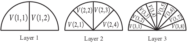
In fact, a straightforward method to solve (6) is to exhaustively search all pairs of and to find the best one. But such a method takes a long time for beam training. To improve the efficiency, beam training based on hierarchical codebooks is adopted [20, 21]. As shown in Fig. 2, a hierarchical codebook typically consists of a small number of low-resolution codewords covering wide angle at the upper layer of the codebook and a large number of high-resolution codewords offering high directional gain at the lower layer of the codebook. The main feature of such a hierarchical codebook can be summarized as: The beams formed by the codewords in the same layer have the same width. The overall coverage of all codewords in the same layer is . Each beam formed by an upper layer codeword covers narrower beams formed by the lower layer codewords, where is called as hierarchical factor [22]. Fig. 2 illustrates an example of hierarchical codebook with and . In general, is the layer of the codebook and is determined by . Compared to the exhaustive tests, the beam training for one data stream based on the hierarchical codebook can reduce the number of tests from to [15]. For example, for an mmWave MIMO system with , and , the training overhead is reduced by . On the other hand, due to the low beam gain of the codewords at the upper layers of the hierarchical codebook, beam training may have lower success rate. Therefore, how to design a hierarchical codebook, especially the upper layer codewords is the focus of this paper.
Once the beam training is finished, and can be designed. Then we send pilot sequences to estimate the equivalent channel matrix which is a product of , and . Once the equivalent channel matrix is estimated, we can design and . Note that we do not directly estimate . We only find the transmit beam and the receive beam best fit for the real channel matrix and then estimate the equivalent channel matrix [22].
II-C Problem Formulation
Note that the codebook is made up of a number of codewords. Therefore, in this paper, we focus on the codeword design. All the codewords in the codebook can be designed based on this work. In this paper, two important issues on codeword design are to be considered. One issue is the design of ideal codewords without consideration of hardware constraints in terms of phase shifter resolution and the number of RF chains. The other issue is the design of practical codewords based on the ideal codeword regarding the hardware constraint.
As in [11] and [15], the design of an ideal codeword with commonly considers the following two objectives:
- 1.
If the steering vector is covered by , the absolute beam gain along the direction of is a constant.
- 2.
If is not covered by , the beam gain is zero.
The beam gain of along is denoted as a function of and as
| (7) |
for . Suppose the coverage of is . Then from the aforementioned two objectives, we have
| (8) |
where the absolute beam gain is determined by and is independent of . This means that is the same for all possible within the beam coverage .
Since it is impossible to find a codeword strictly satisfying (8), we can only design ideal codewords that approach (8) [23]. We will introduce additional phase to to provide additional degree of freedom for ideal codeword design.
Once the ideal codewords are obtained, we can design practical codewords considering the hardware constraints in terms of phase shifter resolution and the number of RF chains [24, 25, 26]. Given an ideal codeword , the design of a practical codeword is essentially to find and , such that
| (9a) | ||||
| (9b) | ||||
| (9c) | ||||
where the constraint of (9b) indicates that the hybrid precoder provide no power gain, and the constraint of (9c) indicates each entry of the analog precoder satisfies the hardware restrictions of the phase shifters. If there are bits for quantized phase shifters, then
| (10) |
In the following, we will propose a two-step codeword design approach for mmWave massive MIMO, which first designs ideal codewords regardless of hardware constraints and then designs practical codewords based on the ideal ones taking the hardware constraints into consideration.
III Ideal Codeword Design
In this section, as the first step of the two-step codeword design approach, we propose a phase-shifted ideal codeword design (PS-ICD) method. Additional phase is introduced to the beam gain to provide extra degree of freedom for ideal codeword design. To determine the additional phase, an alternative minimization method is used, where each iteration of the method is based on a closed-form solution we derive. The proposed PS-ICD can also be extended to design more general beamforming vectors with different beam patterns.
According to (8), the beam coverage of an ideal codeword is , where we may temporarily omit the power constraint of and assume . Then (8) can be simplified as
| (11) |
Denote
| (12) |
where and are both functions of . From (11), we have
| (13) |
Note that the condition in (11) has nothing to do with the phase . Therefore, in our PS-ICD method, we introduce additional phase to increase the degree of freedom.
We define
| (14) |
as a matrix made up of channel steering vectors, where
| (15) |
is the quantized channel AoD with equal interval. Note that the rank of is .
To clearly represent , for , we define a vector , with
| (16) |
The objective of the ideal codeword design is
| (17) |
where . Given , can be obtained by LS as
| (18) |
Direct calculation from (14) yields . Then in (18) can be simplified as
| (19) |
The objective in (17) can be converted to
| (20) |
Note that
| (21) |
Since is predefined, we can further convert (20) to
| (22) |
From (22), only the phases of are involved. Without the constraint of (13), the solution of (22) is the eigenvector corresponding to the largest eigenvalue of . However, it is difficult to solve (22) with the constraint of (13).
Since the phases of are mutually independent, we can use the alternative minimization method to iteratively optimize each phase variable [24, 26]. To be specific, we alternatively optimize until a stop condition is satisfied.
When optimizing by fixing the other entries of , i.e., , we can rewrite (22) as
| (23) |
where
| (24) |
and . Note that the optimization of is now converted as the optimization of real part and imaginary part of , i.e., and , respectively. We have
| (25) |
where
| (26) |
are independent of and , and are fixed once is given. In (III), holds because and , while holds because . Then, (III) can be converted to
| (27) |
As a result, the closed-form solution for (III) can be expressed as
| (28) |
We can obtain as
| (29) |
The stop condition is that the number of iterations equals a predefined maximum number of iterations 11 1 Note that the ideal codeword design problem can also be treated as the design of FIR filter without special specifications [27], which essentially solves a series of convex optimization problems. Since our PS-ICD scheme has close-form solutions, it is much faster than solving convex optimization problems..
We denote as the optimized after finishing the iterations. We can obtain via (16) and then obtain via (19). Since the power constraint of is temporarily omitted in (11), the designed ideal codeword will be
| (30) |
As shown in Algorithm 1, we summarize the steps of PS-ICD algorithm.
In fact, this part of work can be extended to design more general beamforming vectors with various beam patterns, which may be applied for beam training [21]. Given a beam pattern , the beamforming vector can be designed via (30) with obtained via alternative minimization algorithm. In Section V, we will provide two examples to design general beamforming vectors, e.g., triangular beamforming vector and step beamforming vector.
IV Practical Codeword Design
In this section, we will design practical codewords based on the ideal ones designed in Section III, by considering the hardware constraints in terms of phase shifter resolution and the number of RF chains. We will propose a fast search based alternative minimization (FS-AltMin) algorithm for the practical codeword design. [24, 25] In practice, we usually design first, based on which we then design [15][24]. Therefore, we may temporarily ignore (9b) to design since we can always satisfy (9b) by carefully adjusting . Then we have
| (31a) | ||||
| (31b) | ||||
Although the OMP algorithm can be used to solve (31) and obtain a well fit for , it requires a large number of RF chains [15, 25], which occupies large hardware resource and reduce the energy efficiency. In this paper, we focus on how to solve (31) with a small number of RF chains compared to the OMP algorithm.
In the case of , we can simply set to normalize the power and set where
| (32) |
Note that is essentially reduced to be a vector in dimension, since there is only one RF chain. The entries of are mutually independent, indicating that there are limited degrees of freedom that can be explored for pracitcal codeword design.
In the case of , since both and need to be designed, the problem in (31) can be solved by an alternative minimization method, which can minimize (31a) by designing with a fixed and then designing with a fixed [24, 26].
IV-A Initialization
First of all, an initial value is required to start the alternative minimization method. We may initialize either or . Note that there are hardware constraints for while there is no constraint for . We can initialize each entry of by randomly selecting an entry from .
IV-B Design of with a fixed
Given a fixed , the problem in (31) can be converted to
| (33) |
It is a typical least squares problem with the solution expressed as
| (34) |
IV-C Design of with a fixed
Given a fixed obtained via (34), we can focus on the discrete optimization in terms of the quantized phase shifters. Then (31) is converted into
| (35a) | ||||
| (35b) | ||||
It is observed that the entries of the vector are mutually independent, because the entries of are independent to each other. Therefore, the minimization of can be converted to the minimization of the absolute value of each entry of . Then (35) can be converted to subproblems, where the th subproblem can be expressed as
| (36) |
Define
| (37) |
where and are the amplitude and the phase of , respectively. Since the method to solve (36) is exactly the same for different , we can omit the subscript and define . Then (36) can be rewritten as
| (38a) | ||||
| (38b) | ||||
To solve (38), we consider two different cases, and .
IV-C1
In this case, there are two variables and in (38), which can be rewritten as
| (39) |
Denote
| (40) |
where , , and are the amplitude of , the phase of , the amplitude of and the phase of , respectively.
We first ignore the constraints of and solve
| (41) |
Therefore, we have , which is equivalent to
| (42) |
The solutions of (42) can be expressed as
| (43) |
or
| (44) |
If we consider the constrains of , then we can design and as
| (45) |
which is essentially to find two entries from closest to and , respectively.
IV-C2
In case of , there are more than two variables in (38). If we first ignore the constraints in (38b) to solve (38a), just as the case of , the problem will be underdetermined, where there are more unknown variables than the equations. Although the method in [24] can be used to solve the problem without the constraint in (38b), it can only obtain a solution with continuous phase. When the solution is directly quantized, it suffers from the quantization errors. Motivated by the case of , we incorporate the calculation of (45) into the case of and rewrite (38) as
| (46) |
where
| (47) |
with and representing the amplitude and the phase, respectively.
Given , e.g., selecting any entries from as , we can find by
| (48) |
where , using the method as in the case of . Our motivation is that we always leave two degrees of freedom such as and , to best match the given by solving (48). Denote the solution of (48) as . With the given and the computed in (48), we can compute the following objective as
| (49) |
From the above discussion, and can be computed for given . Now (IV-C2) can be converted into the following optimization problem as
| (50) |
where and can be determined with the given via (48). To obtain the solution to (IV-C2), one straightforward method is the exhaustive search, which tests all the combinations of and select the one with the minimum objective. Since each has possibilities, the exhaustive search needs totally tests to obtain the solution to (IV-C2). For example, if and , we need totally tests, which has prohibitively high computation. In this context, sub-optimal search methods are usually adopted to find an appropriate solution to (IV-C2).
Now we propose a fast search (FS) method for the design of based on . The detailed steps are summarized in Algorithm 1. At step 8, we initialize to be , where the superscript “0” represents the number of iterations. In fact, can be set as the corresponding entries of the last computed to guarantee the objective of (31) is always decreasing.
At the th iteration, we determine the value of as follows, where
| (51) |
Note that (51) essentially guarantees that the variables are computed cyclically.
We keep all the entries except to be the same as those in the th iteration, which can be expressed as
| (52) |
Then given these entries, we test all entries from to determine . For each test, given an entry from , denoted as , we obtain and via (48) and then compute . From all of these tests, we find a best satisfying
| (53) |
The solution to (53) is denoted as .
We iteratively perform these steps until the stop condition expressed as
| (54) |
is satisfied. In fact, (54) means the exactly same routine of the iterations is repeated again, which indicates the results thereafter will keep the same. Once is (54) satisfied, we obtain
| (55) |
Then the th row of the designed is as
| (56) |
Finally, we output .
IV-D Design of practical codeword
Now we propose the FS-AltMin algorithm for practical codeword design. Note that the purpose to introduce the name of practical codeword is to be consistent with the ideal codeword in concept. Algorithm 2 summarizes the Subsection IV-A, Subsection IV-B and Subsection IV-C. We iteratively run the algorithms in Section IV-B and Section IV-C to obtain and until the stop condition is satisfied. We may set the stop condition as that a predefined maximum number of iterations is achieved or the entries in do not change any more.
We denote the obtained and by the FS-AltMin algorithm as and , respectively. Note that in (31) we have temporarily ignored the power normalization constraint to simplify the practical codeword design. If the power normalization constraint in (9b) is considered, we set
| (57) |
Finally, the designed practical codeword is
| (58) |
IV-E Complexity Analysis
It can be observed that the FS-AltMin algorithm needs at most iterations. During each iteration, subproblems expressed in (38) need to be solved. For each subproblem, we consider two cases. If , we can get a solution directly via (45) without any iterations. If , we denote the number of iterations to achieve the convergence in (54) as , where we need to compute (49) for times in each iteration. Therefore, the computational complexity in solving (31) is or for or , respectively.
V Simulation Results
Now we evaluate the performance of the proposed two-step codeword design approach for mmWave massive MIMO systems with quantized phase shifters. The ideal codewords are designed with and .
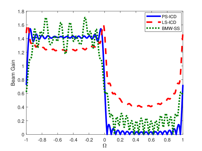
Fig. 3 compares the beam patterns of ideal codewords designed by PS-ICD, BMW-SS [17] and LS-ICD [15] with and . From the figure, PS-ICD is better than BMW-SS and LS-ICD since the codeword designed by PS-ICD is flatter in main lobe and has larger attenuation in side lobe. Table I compares the main lobe variation for different ideal codewords design methods by computing mean-squared errors (MSE) between the designed codewords and the objective in (8). is set to guarantee that the power of codewords is normalized, which can be obtained from Lemma 1 of [11]. From the table, for different , PS-ICD has the smallest variation among the three methods.
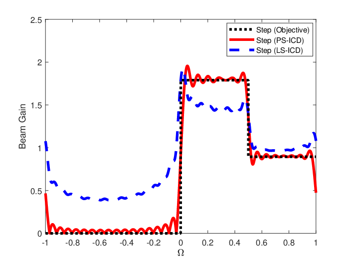
Fig. 4 extends our work to design more general beamforming vectors such as triangular beam and step beam with . Since BMW-SS can not be used to design general beamforming vectors, we compare the beam patterns generated by PS-ICD and LS-ICD. Given the objective beam pattern, e.g., triangular beam or step beam, PS-ICD can better approach the objective beam than LS-ICD. Note that the triangular beam or step beam can be used for beam training by exploiting the overlapped beam patterns of neighbouring beams [21].

| Number of antennnas | PS-ICD | LS-ICD | BMW-SS |
|---|---|---|---|
Fig. 5 compares the beam patterns of practical codewords designed by FS-AltMin, OMP [11] and OMP [15]. To highlight the difference, we only illustrate the main lobe of codewords in Fig. 5. Since PS-ICD performs best among the ideal codeword design methods, we first generate ideal codewords using PS-ICD, where we set the parameters the same as Fig. 3, i.e., and . Then we generate practical codewords using FS-AltMin, OMP [11] and OMP [15] to approach the ideal codeword designed by PS-ICD. We set the same for FS-AltMin, OMP [11] and OMP [15]. The numbers of RF chains for FS-AltMin, OMP [11] and OMP [15] are , and , respectively. In addition, we set for FS-AltMin. From Fig. 5, it is seen that FS-AltMin performs much better than OMP [11] and OMP [15], which means FS-AltMin can better approach PS-ICD than OMP [11] and OMP [15]. Note that compared to FS-AltMin, OMP [15] employs almost four times of the number of RF chains, which implies that FS-AltMin can save large hardware resource aside of generating better beam pattern.
As shown in Fig. 6, we compare the deviation between the designed practical codewords and the ideal codeword with different numbers of RF chains. Since PS-ICD has the best performance for ideal codeword design, an ideal codeword is generated using PS-ICD, where we set the parameters the same as those of Fig. 3, i.e., and . Then we design a practical codeword with FS-AltMin, OMP [11] and OMP [15]. We define
| (59) |
to indicate the deviation between the ideal codeword and the practical codeword . We set the same for FS-AltMin, OMP [11] and OMP [15]. In addition, we set for FS-AltMin. From Fig. 6, it is seen that FS-AltMin performs much better than OMP [11] and OMP [15], which means with the same number of RF chains, the practical codeword designed by FS-AltMin has much smaller deviation than that designed by OMP [11] or OMP [15].

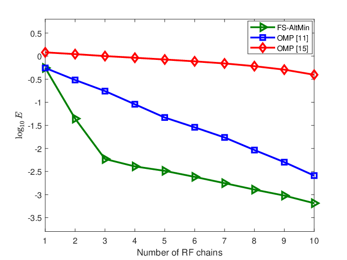

Fig. 7 compares the success rates of beam training using the hierarchical codebooks, where the codewords in these codebooks are designed by three methods. The first two methods are all based on two-step codewords design, where PS-ICD and LS-ICD marked in the parenthesis in Fig. 7 are used to design the ideal codewords. PS-ICD uses FS-AltMin to design the practical codewords with while LS-ICD uses OMP [15] to design the practical codewords with . The last method is BMW-SS, which is designed using the overlapped adding of beams formed by sub-arrays and only considers the design of codewords. We set , and and perform the beam training algorithm based on the hierarchical codebooks proposed in [15]. The definition of success rate is given in (5) and (6). In fact, the success rate in Fig. 7 is determined by the ideal codewords as well as the practical codeword design methods, while the beam pattern in Fig. 5 is only determined by the practical codeword design methods. From Fig. 7, it is seen that the proposed two-step codeword design method outperforms the existing methods. At signal-to-nose ratio (SNR) of 0dB, the proposed method has nearly 15% improvement over BMW-SS. Note that the proposed method can be used to design codewords with arbitrary width of main lobe, which is different from BMW-SS.
VI Conclusion
In this paper, we have investigated the codeword design for mmWave massive MIMO. A two-step codeword design approach has been developed. In the first step, additional phase is introduced to the beam gain to provide additional degree of freedom and the PS-ICD method has been proposed. To determine the additional phase, an alternative minimization method has been used, where each iteration of the method is based on a closed-form solution. The proposed PS-ICD can also be extended to design more general beamforming vectors with different beam patterns. Based on the ideal codewords designed in the first step, in the second step we have proposed a FS-AltMin algorithm that alternatively designs the analog precoder and digital precoder. In our future work, we will try incorporating some good merits of the FIR filter design, e.g. [27], into the beam design in mmWave massive MIMO.
References
- [1] A. Thornburg, T. Bai, and R. W. Heath, “Performance analysis of outdoor mmWave Ad Hoc networks,” IEEE Trans. Signal Process., vol. 64, no. 15, pp. 4065–4079, Aug. 2016.
- [2] B. Wang, F. Gao, S. Jin, H. Lin, and G. Y. Li, “Spatial- and frequency-wideband effects in millimeter-wave massive MIMO systems,” IEEE Trans. Signal Process., vol. 66, no. 13, pp. 3393–3406, Jul. 2018.
- [3] C. Chen, C. Tsai, Y. Liu, W. Hung, and A. Wu, “Compressive sensing (CS) assisted low-complexity beamspace hybrid precoding for millimeter-wave MIMO systems,” IEEE Trans. Signal Process., vol. 65, no. 6, pp. 1412–1424, Mar. 2017.
- [4] J. Choi, B. L. Evans, and A. Gatherer, “Resolution-adaptive hybrid MIMO architectures for millimeter wave communications,” IEEE Trans. Signal Process., vol. 65, no. 23, pp. 6201–6216, Dec. 2017.
- [5] C. Lin and G. Y. Li, “Energy-efficient design of indoor mmWave and sub-THz systems with antenna arrays,” IEEE Trans. Wireless Commun., vol. 15, no. 7, pp. 4660–4672, Jul. 2016.
- [6] C. Lin, G. Y. Li, and L. Wang, “Subarray-based coordinated beamforming training for mmWave and sub-THz communications,” IEEE J. Sel. Areas Commun., vol. 35, no. 9, pp. 2115–2126, Sep. 2017.
- [7] W. Ma and C. Qi, “Beamspace channel estimation for millimeter wave massive MIMO system with hybrid precoding and combining,” IEEE Trans. Signal Process., vol. 66, no. 18, pp. 4839–4853, Sep. 2018.
- [8] Z. Xiao, H. Dong, L. Bai, P. Xia, and X. Xia, “Enhanced channel estimation and codebook design for millimeter-wave communication,” IEEE Trans. Veh. Technol., vol. 67, no. 10, pp. 9393–9405, Oct. 2018.
- [9] X. Xue, Y. Wang, L. Dai, and C. Masouros, “Relay hybrid precoding design in millimeter-wave massive MIMO systems,” IEEE Trans. Signal Process., vol. 66, no. 8, pp. 2011–2026, Apr. 2018.
- [10] R. M¨¦ndez-Rial, C. Rusu, N. Gonz¨¢lez-Prelcic, A. Alkhateeb, and R. W. Heath, “Hybrid MIMO architectures for millimeter wave communications: Phase shifters or switches?” IEEE Access, vol. 4, pp. 247–267, Jan. 2016.
- [11] J. Song, J. Choi, and D. J. Love, “Common codebook millimeter wave beam design: Designing beams for both sounding and communication with uniform planar arrays,” IEEE Trans. Commun., vol. 65, no. 4, pp. 1859–1872, Apr. 2017.
- [12] A. Ali, N. Gonz¨¢lez-Prelcic, and R. W. Heath, “Millimeter wave beam-selection using out-of-band spatial information,” IEEE Trans. Wireless Commun., vol. 17, no. 2, pp. 1038–1052, Feb. 2018.
- [13] X. Sun, C. Qi, and G. Y. Li, “Beam training and allocation for multiuser millimeter wave massive MIMO systems,” IEEE Trans. Wireless Commun., vol. 18, no. 2, pp. 1041–1053, Feb. 2019.
- [14] Z. Xiao, P. Xia, and X. G. Xia, “Codebook design for millimeter-wave channel estimation with hybrid precoding structure,” IEEE Trans. Wireless Commun., vol. 16, no. 1, pp. 141–153, Jan. 2017.
- [15] A. Alkhateeb, O. E. Ayach, G. Leus, and R. W. Heath, “Channel estimation and hybrid precoding for millimeter wave cellular systems,” IEEE J. Sel. Top. Signal Process., vol. 8, no. 5, pp. 831–846, Oct. 2014.
- [16] S. Noh, M. D. Zoltowski, and D. J. Love, “Multi-resolution codebook and adaptive beamforming sequence design for millimeter wave beam alignment,” IEEE Trans. Wireless Commun., vol. 16, no. 9, pp. 5689–5701, Sep. 2017.
- [17] Z. Xiao, T. He, P. Xia, and X. G. Xia, “Hierarchical codebook design for beamforming training in millimeter-wave communication,” IEEE Trans. Wireless Commun., vol. 15, no. 5, pp. 3380–3392, May. 2016.
- [18] R. W. Heath, N. Gonzalez-Prelcic, S. Rangan, W. Roh, and A. Sayeed, “An overview of signal processing techniques for millimeter wave MIMO systems,” IEEE J. Sel. Top. Signal Process., vol. 10, no. 3, pp. 436–453, Apr. 2016.
- [19] J. Wang, Z. Lan, C. Pyo et al., “Beam codebook based beamforming protocol for multi-Gbps millimeter-wave WPAN systems,” IEEE J. Sel. Areas Commun., vol. 27, no. 8, pp. 1390–1399, Oct. 2009.
- [20] A. Alkhateeb, Y. H. Nam, M. S. Rahman, J. Zhang, and R. W. Heath, “Initial beam association in millimeter wave cellular systems: Analysis and design insights,” IEEE Trans. Wireless Commun., vol. 16, no. 5, pp. 2807–2821, May 2017.
- [21] M. Kokshoorn, H. Chen, P. Wang, Y. Li, and B. Vucetic., “Millimeter wave MIMO channel estimation using overlapped beam patterns and rate adaptation,” IEEE Trans. Signal Process., vol. 65, no. 3, pp. 601–616, Feb. 2017.
- [22] Z. Xiao, P. Xia, and X. G. Xia, “Channel estimation and hybrid precoding for millimeter-wave MIMO systems: A low-complexity overall solution,” IEEE Access, vol. 5, pp. 16 100–16 110, 2017.
- [23] J. Zhang, Y. Huang, Q. Shi, J. Wang, and L. Yang, “Codebook design for beam alignment in millimeter wave communication systems,” IEEE Trans. Commun., vol. 65, no. 11, pp. 4980–4995, Nov. 2017.
- [24] X. Yu, J. Shen, J. Zhang, and K. B. Letaief, “Alternating minimization algorithms for hybrid precoding in millimeter wave MIMO systems,” IEEE J. Sel. Top. Signal Process., vol. 10, no. 3, pp. 485–500, Apr. 2016.
- [25] O. E. Ayach, S. Rajagopal, S. Abu-Surra, Z. Pi, and R. W. Heath, “Spatially sparse precoding in millimeter wave MIMO systems,” IEEE Trans. Wireless Commun., vol. 13, no. 3, pp. 1499–1513, Mar. 2014.
- [26] Z. Wang, Q. Liu, M. Li, and W. Kellerer, “Energy efficient analog beamformer design for mmWave multicast transmission,” IEEE Trans. Green Commun. Netw., vol. 3, no. 2, pp. 552–564, June 2019.
- [27] X. Lai and Z. Lin, “Optimal design of constrained FIR filters without phase response specifications,” IEEE Trans. Signal Process., vol. 62, no. 17, pp. 4532–4546, Sep. 2014.