Optimal Mechanism Design for Single-Minded Agents
Abstract
We consider optimal (revenue maximizing) mechanism design in the interdimensional setting, where one dimension is the ‘value’ of the buyer, and the other is a ‘type’ that captures some auxiliary information. A prototypical example of this is the FedEx Problem, for which Fiat et al. 2016 characterize the optimal mechanism for a single agent. Another example of this is when the type encodes the buyer’s budget [8]. The question we address is how far can such characterizations go? In particular, we consider the setting of single-minded agents. A seller has heterogenous items. A buyer has a valuation for a specific subset of items , and obtains value if and only if he gets all the items in (and potentially some others too).
We show the following results.
- 1.
Deterministic mechanisms (i.e. posted prices) are optimal for distributions that satisfy the “declining marginal revenue” (DMR) property. In this case we give an explicit construction of the optimal mechanism.
- 2.
Without the DMR assumption, the result depends on the structure of the minimal directed acyclic graph (DAG) representing the partial order among types. When the DAG has out-degree at most 1, we characterize the optimal mechanism à la FedEx; this can be thought of as a generalization of the FedEx characterization since FedEx corresponds to a DAG that is a line.
- 3.
Surprisingly, without the DMR assumption and when the DAG has at least one node with an out-degree of at least 2, then we show that there is no hope of such a characterization. The minimal such example happens on a DAG with 3 types. We show that in this case the menu complexity is unbounded in that for any , there exist distributions over pairs such that the menu complexity of the optimal mechanism is at least .
- 4.
In addition, we prove that optimal mechanisms for Multi-Unit Pricing (without a DMR assumption) can have unbounded menu complexity as well, and we further propose an extension where the menu complexity of optimal mechanisms can be countably infinite, but not uncountably infinite.
Taken together, these results establish that optimal mechanisms in interdimensional settings are both surprisingly richer than single-dimensional settings, yet also vastly more structured than multi-dimensional settings.
1 Introduction
Consider the problem of selling multiple items to a unit-demand buyer. The fundamental problem underlying much of mechanism design asks how the seller should maximize their revenue. If the items are identical, then the setting is considered single-dimensional. In this case, seminal work of Myerson 1981 completely resolves this question with an exact characterization of the optimal mechanism. The optimal mechanism is a simple take-it-or-leave-it price, and the fact that there are multiple items versus just one is irrelevant. In contrast, if the items are heterogenous, then the setting is multi-dimensional and, unlike the single-dimensional setting, optimal mechanisms are no longer tractable in any sense: [Manelli and Vincent 2007; Briest et al. 2015; Hart and Nisan 2013; Hart and Reny 2012; Daskalakis et al. 2013; Daskalakis et al. 2015].
Very recently, Fiat et al. 2016 identify a fascinating middle-ground. Imagine that the items are neither identical nor heterogeneous, but are instead varying qualities of the same item. To have an example in mind, imagine that you’re shipping a package and the items are one-day, two-day, or three-day shipping. You obtain some value for having your package shipped, but only if it arrives by your deadline (which is one, two, or three days from now). We can think of the input as being a (correlated) two-dimensional distribution over (value, deadline) pairs.
The FedEx Problem is a special case of single-minded valuations: a buyer has a valuation for a specific subset of items , and obtains value if he gets any superset of , and 0 otherwise. To have an example in mind, imagine that a company offers internet, phone service, and cable TV. You have a value, , and are interested in getting internet service. So you value options such as exclusively internet service, internet/phone service, or internet/cable, and so on, at . For any option that does not include internet you get a value of zero (so we again think of the input distribution as a two-dimensional distribution over (value, interest) pairs).
An alternative perspective to single-minded valuations is that there is a partial order on the set of possible interests a buyer may have. The partial order is just the one induced by set inclusion. The FedEx problem has totally-ordered items: one-day shipping is at least as good as two-day shipping is at least as good as three-day shipping, and every buyer agrees. In fact, any partial order can be induced from set inclusion, so the two settings are equivalent (see Observation 2 in Appendix G). It turns out that the partial order view is more useful from a mechanism design perspective, therefore we will use that view for the rest of the paper.
The following problem can also be interpreted as a partially-ordered setting: Suppose that each buyer has a publicly visible attribute which the seller can use to price discriminate. E.g., the buyer could be a student, a senior, or general-admission. Or, the buyer could be a “prime member” or a “non-prime member.” However, buyers with certain attributes can disguise themselves as having other attributes, given by a partial order. For example, a prime member could disguise as a non-prime member, but not vice-versa. Then if item is a movie ticket redeemable by anyone who can disguise themselves as having attribute , the items are partially-ordered.
1.1 Main Results
Fiat et al. 2016 give a characterization of an optimal mechanism for the FedEx problem, and our goal is to understand the generalizability of this characterization, in particular to the partially ordered setting. Towards this, we first describe the FedEx characterization and what a generalization could look like. A deterministic mechanism sets a posted price for each shipping option, and the buyer picks the option he prefers (if any). Clearly, it makes sense for the prices to be non-increasing in -day shipping. The FedEx solution is recursive: start with the price on day 1 (as a variable), and constrain the price on day 2 to be weakly lower, and so on. When the distributions satisfy the Declining Marginal Revenue (DMR)11 1 A one-dimensional distribution satisfies Declining Marginal Revenues if is concave. See Devanur et al. 2017 for examples and more discussion. For example, uniform distributions are DMR, along with any distribution of bounded support and monotone non-decreasing density. property, this strategy actually results in deterministic prices that are optimal. Without any distributional assumption, one might have to resort to lotteries: the buyer gets the item only with some probability. The first day price is still deterministic, but for the second day, the mechanism offers a lottery such that the expected price for full service is weakly lower. It turns out that we only need to randomize between two options. Recursively, every option on day may split into two options on day , so we might have at most options on day , and options overall (and examples exist where options are necessary [Saxena et al. 2018]).
So our starting point is a hope that similar recursive ideas can characterize optimal auctions beyond the totally-ordered FedEx setting. Some terminology is useful here to understand precisely what this might mean. We use the directed acyclic graph (DAG) representation of a partial order: an edge from to implies is preferred over . The DAG is minimal: if and are edges then is not an edge. The DAG for the FedEx problem goes right to left, i.e., it has edges for from 1 to . A recursive approach for a DAG would look like this: start with a sink, set a deterministic price, and use this to constrain the prices (either deterministically or in expectation, based on the distributional assumption) for its predecessors and so on. The goal of this paper is to understand Will something like this work for partially-ordered items?
DMR:
Under the DMR assumption, this strategy for pricing works in any DAG (Theorem 4 in Appendix C). We start from the sink nodes and recursively constrain the price of a node to be at most the minimum among the prices of all its successors. Our proof that this procedure works employs LP duality, and a significantly more involved procedure to set appropriate dual variables than in [10]. The fact that optimal mechanisms are deterministic subject to DMR matches prior work for totally-ordered settings [5; 10; 8; 9].
Out-degree 1:
The FedEx strategy still works when the minimal DAG has out-degree at most 1, without any distributional assumptions (Theorem 5 in Appendix D). Compared to the DMR case, we now have to deal with lotteries but when we process a node, there is exactly one successor that constrains the lotteries for this node, in exactly the same way as in FedEx.
3 node DAG:
The minimal example where the out-degree is 2 is a three-node DAG with nodes , and , and edges and . One might hope that the following recursive strategy would work (after all, the graph is still a DAG, and should be amenable to recursive arguments): set prices deterministically for and and use the minimum of the two to constrain the expected price for . Note that if there were no item , this would match precisely the FedEx solution.
It turns out that this idea fails horribly, for the following (very high-level) reason. With just two items ( and ), the price of transparently constrains what prices we can set for (the expected price for must be lower). So when optimizing the price of , we can take this into account. With three items, it’s no longer clear how the price of constrains the price of . Certainly, the expected price for must be lower, but perhaps a stronger constraint is already implied by the price of . Therefore, one cannot separately optimize the price of without knowing the price of .
Indeed, this intuition actually manifests into a lower bound: it is not only challenging to jointly optimize the prices of together, but the optimum may no longer be deterministic at all! Specifically, for any integer , there exist value distributions for this 3-node DAG for which the unique optimal mechanism presents different lotteries to the buyer (Theorem 1). Essentially, there is no hope for a FedEx style solution even for this minimal case. We focus the technical presentation of our paper on this result.
Finiteness of menu complexity:
The use of menu complexity lower bounds to ascertain complexity of mechanisms is not new: Manelli and Vincent 2007; Daskalakis et al. 2015 show that the optimal mechanism for the multi-dimensional setting might have uncountable menu complexity—this holds even for just two items with additive valuations, and even when the item values are drawn independently from absolutely bounded distributions. This dichotomy serves as one fundamental difference between single-dimensional and multi-dimensional settings.
Within the context of these results, we ask if we can get an infinite (uncountable or countable) menu complexity for the partially-ordered setting as well. A natural strategy is to take the limit of our construction as the number of randomizations goes to infinity. Somewhat surprisingly, the example then collapses and has a deterministic price as optimal. We show that this is no coincidence: that the menu complexity for the three item case is always finite (Theorem 2).
Summary:
The main technical takeaway from our results is a thorough understanding of optimal mechanisms in interdimensional settings beyond FedEx through broadly applicable tools. Our theorem statements use the language of menu complexity, but only to distinguish among mechanisms with bounded, unbounded, or infinite menu complexity. The main conceptual takeaway is that optimal auctions for single-minded valuations lie in a space of their own: significantly more complex than optimal single-dimensional auctions, or even optimal auctions for totally-ordered valuations, yet more structured than optimal multi-dimensional auctions.
Known Menu Complexity Results for Optimal Mechanisms with One Buyer
| One Item | FedEx | Single-Minded, 3 Items | Multi-Unit | Coordinated, 3 Items | Additive | |
|---|---|---|---|---|---|---|
| Det. under DMR | N/A | ✓ | ✓ | ✓ | ✗ | N/A |
| Lower Bound | 1 | unbounded | unbounded | countably infinite | uncountable | |
| Upper Bound | 1 | finite | — | countably infinite | uncountable |
Bold results are from this paper.
1.2 Additional results
We postpone all details about our proofs to the technical sections, but highlight one result of independent interest that we develop en route. Our problem can be phrased as a continuous linear program, and all of our proofs require reasoning about the dual. In particular, developing our lower bound construction (instances with unbounded menu complexity) consists of two parts: First, we construct a candidate dual for which a primal exists satisfying complementary slackness, and for which every primal satisfying complementary slackness has menu complexity . Second, we prove that there exists a distribution for which is a feasible dual (and combining these two claims means that every optimal mechanism for this input has menu complexity ). Analyzing through complementary slackness is technically interesting, and captures all of the insight one would hope to gain from the construction. Reverse engineering an instance for which is feasible, however, is technically challenging yet unilluminating. On this front, we prove a “Master Theorem,” stating essentially that every candidate dual is feasible for some input distribution (Theorem 9). This allows the user (of the theorem) to reason exclusively about primals and duals, letting the Master Theorem map the candidate pair back to an instance for which they are feasible. In some sense, the Master Theorem formally separates the insightful analysis from the tedious parts.
Of course, one should not expect this theorem to hold in general multi-dimensional settings (in particular, one key property that enables our Master Theorem is a “payment identity,” which general multi-dimensional settings notoriously lack—this is a further example of how our setting lies in-between single- and multi-dimensional), but the Master Theorem is quite generally applicable for problems in this intermediate range. In addition, because the Master Theorem takes care of guaranteeing that distributions corresponding to some dual will exist, this result also emphasizes the strength of reasoning about duals in similar settings.
Finally, beyond our main results, we prove two additional results using the same tools. First, we apply our lower bound techniques to show that the menu complexity of the Multi-Unit Pricing problem [9] is also unbounded (Theorem 12 in Appendix I). Multi-Unit Pricing is also a totally-ordered setting, where the items correspond to copies of a good (item one is one copy, item two is two copies, item three is three copies). The difference from FedEx is that if the buyer is interested in two copies but gets one, they get half their value (versus zero). Second, we propose a generalization beyond totally-ordered settings which we call coordinated valuations, and again characterize the menu complexity of optimal mechanisms for one instance of three items (which can be countably infinite, but not uncountable, see Appendix J).
1.3 Related Work
Single-minded valuations are a well-known model (e.g. [Lehmann et al. 2002]). Most work in this model pertains to welfare maximization in more complex settings, such as combinatorial auctions. Other work assumes that the buyer’s interest is publicly known; in this case, the buyer is single-parameter, and a single-buyer revenue maximization problem reduces to Myerson.
The most related line of works has already mostly been discussed. The FedEx Problem considers totally-ordered items (in our language), as does Multi-Unit Pricing and Budgets [Che and Gale 2000; Fiat et al. 2016; Devanur et al. 2017; Devanur and Weinberg 2017]. The present paper is the first to consider partially-ordered items. In terms of techniques, we indeed draw on tools from prior work. All three prior works employ some form of duality. Our approach is most similar to that of Devanur and Weinberg 2017 in that (1) both are the only works to use the analysis from [4] to characterize optimal mechanisms rather than obtain approximations, and (2) we also perform “dual operations” rather than search for a closed form. However, as the single-minded setting is much more complicated, we extend the techniques to handle this setting.
Also related is a long line of work which aims to characterize optimal mechanisms beyond single-dimensional settings. Owing to the inherent complexity of mechanism design for heterogeneous items, results on this front necessarily consider restricted settings [Laffont et al. 1987; Giannakopoulos and Koutsoupias 2014; McAfee and McMillan 1988; Daskalakis et al. 2013; Daskalakis et al. 2015; Haghpanah and Hartline 2015; Malakhov and Vohra 2009]. From this set, the most related are Haghpanah and Hartline 2015; Malakhov and Vohra 2009, who also considered settings where all consumers prefer (e.g.) item to item , but there are no substantial technical connections.
There is also a quickly growing body of work regarding the menu complexity of multi-item auctions. Much of this work focuses on settings with heterogeneous items [Briest et al. 2015; Hart and Nisan 2013; Babaioff et al. 2017; Wang and Tang 2014; Daskalakis et al. 2015; Gonczarowski 2018]. Very recent work of [23] considers the menu complexity of approximately optimal mechanisms for the FedEx Problem (for which [10] already characterized the menu complexity of exactly optimal mechanisms). On this front, our work places partially-ordered items (where the menu complexity is finite but unbounded) distinctly between totally-ordered items (where the menu complexity is bounded) [10], and heterogeneous items (uncountable) [7]. Previously, no settings with this property were known.
1.4 Roadmap
Our paper contains four main results, although we view the primary contributions as (3) and (4):
- 1.
In Appendix C, we prove Theorem 4, which explicitly constructs a deterministic optimal auction for partially-ordered items when all marginals are DMR.
- 2.
In Appendix D, we prove Theorem 5, which extends the recursive FedEx algorithm for totally-ordered items to partially-ordered items when minimal DAGs with outdegree at most one.
- 3.
We focus our technical presentation on the ideas necessary for Theorem 1, which establishes that any partially-ordered instance for which some node in the minimal DAG has outdegree at least two, the menu complexity of the optimal mechanism may be unbounded. In Section 2 we provide the minimal preliminaries to understand the main ideas behind our proof of this result (full preliminaries in Appendix A). In Section 3 we overview the key duality aspects. In Section 4 we give a brief overview of the proof of Theorem 1. The full proof is in appendix E.
- 4.
Finally, we also establish that the menu complexity of optimal mechanisms for this minimal -item instance is always finite. The main ideas appear in Section 4, and a full proof of Theorem 2 appears in Appendix F.
Outside of our main results, Appendix H presents our “Master Theorem” (Theorem 9), which is of independent interest for future work on mechanism design with totally- or partially-ordered items. In Appendix I and Appendix J we display the applicability of our techniques for related settings such as Multi-Unit Pricing (Theorem 12) and coordinated values (Theorems 14, 16, 17), respectively. Section 5 presents our conclusions and discusses future work.
2 Preliminaries
In the interest of presentation, we’ll provide the minimum preliminaries here for the reader to understand the key ideas. In Appendix A, we provide full preliminaries, including additional intuition, and covering prior work (such as [10; 8]). Many of the facts we will use are stated here without proof (proofs are given in Appendix A).
2.1 A Minimal Instance
We focus on the three-item case with items where and , but and . That is, if a buyer is interested in item , they are content with or . If they are interested in , they are content only with (ditto for ). There is a single buyer with a (value, interest) pair , who receives value if they are awarded an item (that is, or ). This is the minimal non-trivial example of a partially-ordered setting. A menu-complexity lower bound for this example applies to any partially-ordered setting that contains an item with at least two incomparable items that dominate (which includes every single-minded valuation setting with at least items).
An instance of the problem consists of a joint probability distribution over , where is the maximum possible value of any bidder for any item.22 2 Note that the multi-dimensional instances with uncountable menu complexity are also supported on a compact set: . So our results are not merely a product of compactness. We will use to denote the density of this joint distribution, with denoting the density at . We will also use to denote , and to denote the probability that the bidder’s interest is .
We’ll consider (w.l.o.g.) direct truthful mechanisms, where the bidder reports a (value, interest) pair and is awarded a (possibly randomized) item. Further, as observed in Fiat et al. 2016, it is without loss of generality to only consider mechanisms that award bidders their declared item of interest with probability in , and all other items with probability .33 3 To see this, observe that the bidder is just as happy to get nothing instead of an item that doesn’t dominate their interest. See also that they are just as happy to get their interest item instead of any item that dominates it. It will also make this option no more attractive to any bidder considering misreporting. So starting from a truthful mechanism, modifying it to only award the item of declared interest or nothing cannot possibly violate truthfulness. Note also that this modification maintains optimality, but could impact the menu complexity up to a factor of # items. As we only consider distinctions between bounded, unbounded, and infinite, this is still w.l.o.g. For a direct mechanism, we’ll define to be the probability that item is awarded to a bidder who reports . Our goal is to find the revenue-optimal allocation rule— defined for all with payment determined by the allocation rule—such that the mechanism is incentive-compatible. The menu complexity of a direct mechanism refers to the number of distinct pairs such that there exists a with .
2.2 Incentive Compatibility, Revenue Curves, and Ironing
As observed in [10], it is without loss of generality to only consider mechanisms that award bidders their declared item of interest with probability in , and all other items with probability . Also observed in [10] is that Myerson’s payment identity holds in this setting as well, and any truthful mechanism must satisfy (this also implies that the bidder’s utility when truthfully reporting is ). This allows us to drop the payment variables, and follow Myerson’s analysis. Fiat et al. observe that many of the truthfulness constraints are redundant, and in fact it suffices to only make sure that when the bidder has (value, interest) pair they:
- •
Prefer to tell the truth rather than report any other . This is accomplished by constraining to be monotone non-decreasing (exactly as in the single-item setting).
- •
Prefer to tell the truth rather than report any other . By , we mean all items such that , but there does not exist a with . This is accomplished by constraining (as the LHS denotes the utility of the buyer for reporting and the RHS denotes the utility of the buyer for reporting ). Note that this is equivalent to saying that the area under ’s allocation curve should be at least as large at every as the area under ’s allocation curve.
All of these constraints together imply that also does not prefer to report any other .44 4 For example, if prefers truthful reporting to reporting where , and prefers truthful reporting to reporting , then since gets the same utility for reporting as type does for truthfully reporting, prefers truthful reporting to reporting . We conclude this section with some standard definitions and observations.
Definition 1 (Revenue Curve).
The revenue curve for an item with CDF is a function that maps a value to the revenue obtained by posting a price of , for a single item, when buyer values are drawn from the distribution Formally, . We say that a revenue curve is feasible if there exists a distribution that induces it. The monopoly reserve price of the revenue curve is .
Definition 2 (Virtual Value).
Myerson’s virtual valuation function is defined so that . Observe that . When clear from context we will omit the subindex .
Definition 3 (DMR).
We say that a marginal distribution of values satisfies declining marginal revenues (DMR) if is concave, or equivalently, if is monotone non-decreasing.
When the marginal distributions do not all satisfy the DMR assumption, we instead need to iron the distribution, an analogue to Myersonian ironing.
Definition 4 (Ironing).
The ironed revenue curve denoted for a revenue curve is the least concave upper bound on the revenue curve .55 5 We emphasize that this work irons the revenue curve with values on the -axis. Classical one-dimensional ironing (to yield Myersonian ironed virtual values) is done on the revenue curve with quantiles on the -axis. A point is ironed if . We say that is an ironed interval if , , and for all , where if , then and are the lower and upper endpoints of the ironed interval, respectively.
An ironed revenue curve is depicted in Figure 1. By the definition of concavity, if is ironed, then where , , and are unironed. Importantly, observe that setting price to a consumer drawn from yields revenue . Yet, if we set price with probability and with probability , we will get revenue . One can check that this is precisely the allocation and payment

3 Duality
In this section, we briefly overview the bare minimum duality preliminaries required. Full duality preliminaries are provided in Section A.3-A.5.
3.1 Dual Terminology.
In this section, we introduce pictorial representations (Figures 2 and 3) of key aspects of a dual solution and define terminology relevant to the dual.

The primal variables are for all , . Recall that we use to refer to the utility of . The dual variables are , for all , and . We first explain the role of these dual variables, and then describe the Lagrangian relaxation obtained using these dual variables.
Dual Variable .
The dual variables correspond to incentive constraints between types of the same interest but different value. This dual controls ironing, as explained below. This really does correspond to ironing in the classical Myerson sense, only in value space.
An oval (as depicted in Figure 2) represents an ironed interval, a region where the dual variable is non-zero.
- •
(Ironing) We say a type is ironed, or that is ironed in item , if .
- •
(Ironed Intervals) For any type , the ironed interval containing in is defined by the bottom end point and the top end point . Then for all , type is ironed, , and .
As we will see later, dual best response (condition (4)) requires that if then . In other words, the allocation rule must be constant over ironed intervals. For any value , an optimal allocation must satisfy that .
Dual Variable .
The dual variables correspond to incentive constraints between types of the same value but different interest.

In Figure 3, a horizontal arrow into item (or ) at indicates that (or ) is non-zero. We write the following statements for .
- •
(Flow) We will call the value of the “flow into ” or the “flow into at .” When we focus on the minimal partial-order example, we infer that flow into or comes from in our figure.
Dual best response (condition (5)) requires that for , if then , or equivalently, : a type with value should have the same utility in and . Sending flow across interests forces the corresponding utilities to be the same.
Virtual Values.
We will define a new variable, for all , and we will call the product the virtual value.66 6 Whether we refer to as the virtual value or reflects whether we iron in the quantile space or the value space. Once again, this is a generalization of Myerson’s virtual value function to this more general setting.
Figure 2 has a vertical axis ranging over values from (at the bottom) to (at the top), with a label of the item of focus at the top. The point on the axis for any represents the virtual value .
Of particular interest to us is the region where the virtual value is 0 because this is the region (and the only region) for which a primal satisfying complementary slackness can have a randomized allocation. This is an interval if is monotone in (our solution ensures it is; details in Appendix A.5).
- •
(Endpoints of Zero Region) We define the bottom end point of the zero virtual value region in by and the top end point .
In Figure 2 the horizontal black lines and signs indicate where the virtual values shift from positive sign to zero, , and from zero to negative sign, . Primal best response requires the allocation to satisfy for (condition (2)) and for (condition (3)).
3.2 The Lagrangian Dual.
The quality of a primal solution is measured by how well it solves the following Lagrangian relaxation induced by . The quality of a dual solution is measured by the value of its induced Lagrangian relaxation. A dual is better if the value of its induced Lagrangian relaxation is smaller.
| Variables: | |||
| Maximize | |||
| subject to |
| (1) |
Before continuing, lets parse the Lagrangian relaxation. The only remaining constraints are that , and the objective is a linear function of these variables. This immediately implies that the solution to this LP relaxation will set whenever , and whenever . This implies that if there is any randomization, i.e., then it must be that . The details of the definition of are not so important here. (However, note that in the definition of , the term refers to the derivative of .)
3.3 Complementary Slackness.
Under strong duality, a (primal, dual) pair is optimal if and only if the primal and dual satisfy complementary slackness. In addition, if a dual is optimal, i.e. satisfies complementary slackness with some primal, then any primal is optimal if and only if it satisfies complementary slackness with . Let’s review complementary slackness in our setting. A primal and dual satisfy complementary slackness if and only if:77 7 One can interpret these conditions as saying that the primal is an optimal solution to the Lagrangian relaxation, and the dual is the worst possible Lagrangian relaxation for the primal.
| (Primal best response) | (2) | |||||
| (3) | ||||||
| (Dual best response) | (4) | |||||
| (5) |
That is, a primal is a best response to a dual if all with positive virtual value are awarded the item, and all with negative virtual value are not. A dual is a best response to a primal if whenever a dual variable is non-zero, the corresponding local IC constraint is tight. The entire technical aspect of this paper is using the constraints imposed by complementary slackness in (2-5) to reason about optimal mechanisms and their menu complexity.
4 Menu Complexity
We provide here the key ideas behind the construction that forms our lower bound and the proof of our upper bound. Full details are provided in Appendix E and Appendix F respectively.
4.1 Menu Complexity is Unbounded: A Gadget and Candidate Instance
In this section, we provide a gadget that will be used in our menu complexity lower bound, and successively chain copies of it together to build our full construction. For one instance of our gadget, we provide a concrete potential dual, and prove that any allocation rule satisfying complementary slackness with it must have two distinct allocation probabilities. In order for this example to establish a menu complexity lower bound of two, we must additionally:
- •
Establish that there exists a distribution for which our dual is feasible. This is not covered in this section, and is deferred to our Master Theorem (Theorem 9).
- •
Establish that there exists an allocation rule which satisfies complementary slackness with this dual, thereby establishing that the dual is optimal (and any optimal allocation rule must satisfy complementary slackness with it). This is also not covered in this section, and is deferred to Appendix F.
We begin below with our gadget, then successively chain copies together to establish a menu complexity lower bound of for any . We recall the following facts established in the previous section:
- 1.
- 2.
A in any graphics into at represents flow in. When there is flow into both and at the same point , this implies that . (CS5)
- 3.
A point in the middle of an oval in any graphics represents that is contained in the interior of an ironed interval, and implies that where is the bottom of the oval. (CS4)
4.1.1 Step One: the base gadget and a lower bound of .

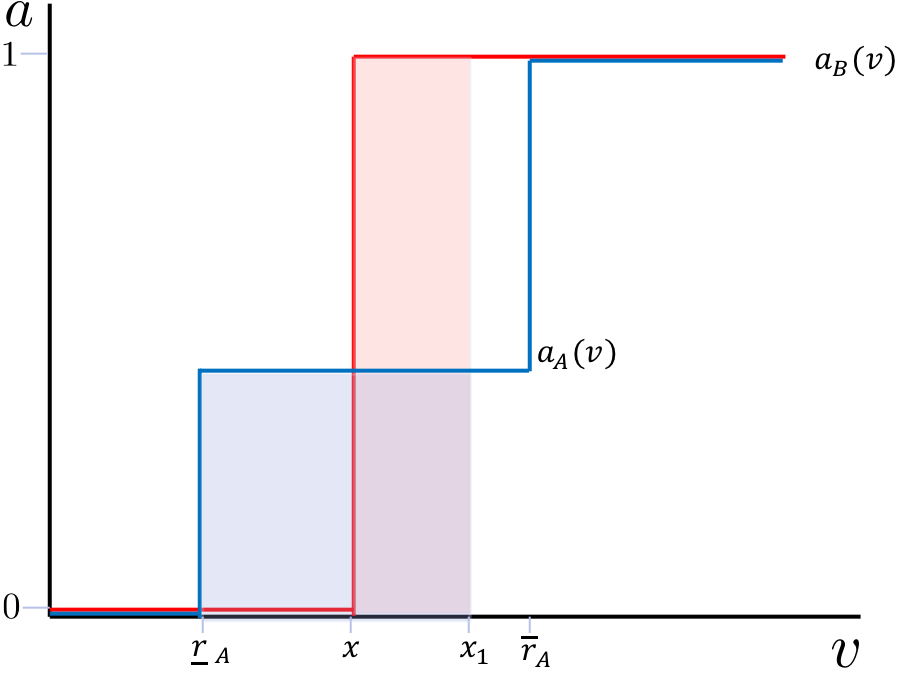
Our base case example is depicted in Figure 4. We note each feature, and how it ties our hands with respect to the allocation rule via complementary slackness.
- •
In item , there is a single point for which . That is, . Then (CS2) implies that for .
- •
There is flow into both items and at . That is, . (CS5) implies that and must be equally preferable at , that is, . Note that for , hence . Then to have , because is monotone, it must be the case that .
- •
The point has and is in an ironed interval where , that is, this ironed interval is the entire region of values that have virtual value zero in item and it contains both and . Because is in an ironed interval in , then the allocation is constant, so , which we have already established must be positive.
- •
For whatever value that takes on, because , to satisfy equal preferability at (again, that ), we must have , resulting in at least two distinct non-zero probabilities of allocation.
To complete the example, (1) there is no other flow: for all , , and (2) item is unironed everywhere: for all . This base gadget forces randomization for the allocation of item because the utility of must be equal at and , but the allocation of item must be zero below , while the allocation of item must be non-zero.
4.1.2 Step Two: two chains and a lower bound of .
Our second example (see Figure 5) contains the relevant features from the first example, but extends it to add an additional constraint: we replace the condition with an ironed interval where . We claim that this example requires us to randomize on both items. Intuitively, this is because we now have two constraints on utilities that must be satisfied, so two degrees of freedom seems necessary.
- •
There is flow into both items and at : . (CS2) implies that for , so to satisfy equal preferability, we must have .
- •
The point has and is in an ironed interval where . As is in an ironed interval in , then the allocation is constant, so .
- •
There is flow into both items and at : . Since —it lies in the ironed interval in , so )—then to satisfy equal preferability at , we must have .
- •
The point has and is in an ironed interval where . As is in an ironed interval in , then the allocation is constant, so .
- •
For whatever value that takes on, because , then to satisfy equal preferability at (that ), we must have .
- •
For whatever value that takes on, because , then to satisfy equal preferability at (), we must have , resulting in at least three distinct non-zero probabilities of allocation.
Again, (1) there is no other flow: for all , , and (2) item is unironed everywhere: for all .
Observe that in both examples, we reason from where we have one item with positive virtual value and the other with virtual value zero downward that, in order to satisfy a number of equal preferability constraints, because ironed intervals force the allocation to be constant, then at every point, the allocation must be non-zero. Then, we reason upward that, because the ironed intervals are interleaving between the items and never aligned, the allocation must strictly increase at each point of interest in order to satisfy equal preferability. This is precisely the reasoning we will use to construct and prove an arbitrarily large instance and menu.


Right: If , then (the blue region is smaller than the red), which violates complementary slackness.
4.1.3 Step Three: four chains and a lower bound of .
In this section, we take one more step towards our general construction. The first example presents our base gadget, and the second example chains two copies together. In this section, we simply confirm how the gadgets interact as we chain more and more together, bouncing back and forth from to .


Right: If , then (the blue region is smaller than the red), which violates complementary slackness via Fact 2 at .
Nonzero allocation probabilities.
First, we see that the allocation at every ironed value such that must be nonzero: . The argument holds for each of , , and . Below we iterate the same argument made in the two previous sections, skipping some details.
Essentially, if any of these allocations must be positive, it forces the rest of them, working downwards, to be positive. And, by Fact 1, , so . Hence the rest of the implications follow, so the allocation must be nonzero throughout this region.
Distinct allocation probabilities.
Now, given that the allocation must be nonzero at every point in this range, we argue that it must be distinct at all of the points of interest. Fix some nonzero , and note by Fact 3 that for all . By Fact 1, for . Because , then to have , since and , then we must have a distinct . This is depicted on the right side in Figure 6. Then, by Fact 3, .
The argument extends inductively for , and : we show it with . Note that and suppose the inductive hypothesis of , where and by Fact 3. Hence . Then in order to have , we must have .
The result is four distinct allocation probabilities in these four regions, and five in total (including the deterministic option to get the item w.p. one). Essentially, this example only has two ironed intervals in and each with four points of interest. Our full construction below lets the number of ironed intervals grow with .
4.1.4 Final Step: chains and a lower bound of .
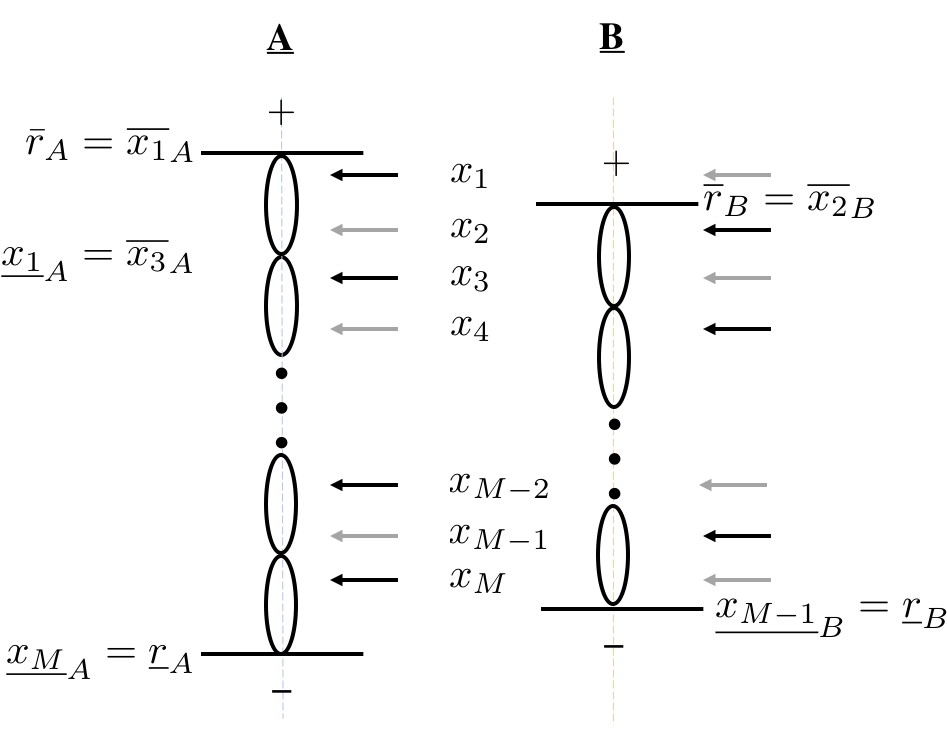
It is possible to extend the examples above by continuing to interleave ironed intervals with flow coming in. The combination of the equal preferability constraints and the inability to increase the allocation in the middle of an ironed interval is what requires us to randomize differently within each interval, forcing any number of menu options. Details are given in Appendix E, where we formally define this “top chain” structure (Definition 7) and construct the candidate dual instance, which is depicted in Figure 7. For example, our first example has a top chain of length one, the second of length two, and the third of length four. Theorem 2 proves that there exists a primal instance that satisfies complementary slackness with the defined dual. This proves both that our dual is optimal, and thus any optimal primal must satisfy complementary slackness with it, giving us Theorem 1.
Theorem 1.
Mechanisms that satisfy complementary slackness with a dual containing a top chain of length have menu complexity at least . Moreover, for all , there exists a distribution over three partially-ordered items for which a dual with top chain of length is feasible.
The “Moreover, …” part of the theorem is due to our Master Theorem (Theorem 9). The formal statement is a bit technical, and can be found in Appendix H.
4.2 For Three Items, Menu Complexity is Finite: Brief Highlight
In Appendix F, we discuss our approach for characterizing the optimal mechanism for our 3-item minimal instance. We prove essentially that the interleaving of ironed intervals used in the construction of the previous section is the worst case (in terms of menu complexity). We do this by specifying a subclass of optimal duals (that we call best duals) using two new dual operations, double swaps and upper swaps. We then leverage the structure of the best duals to give an algorithm that recovers the optimal primal from any best dual, and prove that the resulting mechanism has finite menu complexity.
Theorem 2.
For any best dual solution, the primal recovery algorithm returns a primal with finite menu complexity that satisfies complementary slackness (and is therefore optimal).
We conclude with one vignette regarding how the menu complexity can be unbounded but not infinite. Two crucial aspects of the “top chain” structure from our examples (generalized in Figure 7) are that: (1) the ironed intervals for and are interleaving—this is what “keeps the chain going” and (2) the sequences for and terminate at different bottom endpoints. The latter is a bit subtle, but the idea is that if the two chains terminate at the same bottom endpoint , then this entire process can be aborted and simply setting as the reserve for all items satisfies complementary slackness. So while in principle, this top chain structure could indeed be countably infinite, it cannot also satisfy (1) and (2). This is because the monotone convergence theorem states that both chains do indeed converge to some bottom endpoint, and interleaving then guarantees that this bottom endpoint must be the same.
4.3 One Last Example
In this section, we construct an example by applying the Master Theorem (Theorem 9) to the dual in Figure 6. The customer prior distribution in the example consists of the marginal distributions depicted in Figure 8. The distributions for and do not satisfy DMR, and, using the ideas from the previous subsections, we will see that the optimal mechanism is randomized.


We can use the revenue curve procedure from Appendix B to determine the optimal pricing for this example. It produces the curves in Figure 8, telling us that the optimal price to set on item is , which will result in prices of on item and 8 on item . This gives . However, as we have seen in Section 4.1, for the dual in Figure 6 (which corresponds to this distribution) to satisfy complementary slackness with a mechanism, the mechanism must have a good deal of randomization.
In Section 4.1, we reasoned that the allocation probability must be distinct at each of the points , , and . We also saw that if we fixed the allocation at , there was only one way to satisfy the rest of the complementary slackness constraints, forming a system of equations. The primal recovery algorithm described in the proof of Theorem 2 goes through solving this system of equations, ensuring that any other additional complementary slackness constraints are met, and that no pathological structures that might prevent a solution from existing can arise. Applying this algorithm to our example results in the following optimal randomized mechanism:
The mechanism achieves a revenue of 3.2, which is slightly more than that of the best deterministic mechanism.
5 Conclusions
We study optimal mechanisms for single-minded bidders, and show that the menu complexity of optimal mechanisms is unbounded but finite for three items. Recall that for three identical items, the menu complexity is 1, for totally-ordered items the menu complexity is at most 7, and for heterogeneous items the menu complexity is uncountable. So our setting fits nicely ‘‘in between’’ totally-ordered and heterogeneous by this measure. By fuzzier measures of complexity, the same is true too: for identical items, the optimal mechanism has a clean closed-form description. For totally-ordered items, the optimal dual has a closed form, and the primal can be recovered by a simple algorithm as a function of this dual. For partially-ordered items, the optimal dual is unlikely to have a closed form, but can be characterized in terms of properties it must satisfy, and the primal can still be recovered algorithmically88 8 Contrast this with [Cai et al. 2012], which only claims that by solving a linear program, an optimal mechanism for heterogenous settings can be found in time polynomial in the type space. as a function of this dual. For heterogeneous items, optimal mechanisms are pure chaos. And, like other settings that can be placed fundamentally in between single- and multi- dimensional settings (e.g., FedEx and MUP), we prove that the optimal mechanism is deterministic under DMR in the partially-ordered setting.
We also provide extensions—menu complexity of MUP (Theorem 12, Appendix I) and of coordinated values (Theorems 14, 16, 17, Appendix J)—proving the usefulness of our techniques beyond our setting.
Many interesting open directions remain. First, general menu complexity upper bounds—for the single-minded setting, the Multi-Unit Pricing setting, and the coordinated valuations setting. The techniques we use in this paper focus on characterizing the optimal dual and recovering the optimal mechanism for the three-item single-minded setting; this approach appears to be far too detailed and focused on characterizations to be extended. We expect new ideas to be needed.
Second, the question of menu-complexity lower bounds for any of these three settings for approximately-optimal mechanism are wide-open. Is the separation from FedEx still as large when we only require approximately-optimal revenue?
Both directions of research would further fill out this rich spectrum, which until only recently was but thought to be a dichotomy between single-dimensional and heterogenous.
References
- Babaioff et al. [2017] Moshe Babaioff, Yannai A. Gonczarowski, and Noam Nisan. The menu-size complexity of revenue approximation. In Proceedings of the 49th Annual ACM SIGACT Symposium on Theory of Computing, STOC 2017, pages 869–877, New York, NY, USA, 2017. ACM. ISBN 978-1-4503-4528-6. doi: 10.1145/3055399.3055426. URL http://doi.acm.org/10.1145/3055399.3055426.
- Briest et al. [2015] Patrick Briest, Shuchi Chawla, Robert Kleinberg, and S Matthew Weinberg. Pricing lotteries. Journal of Economic Theory, 156:144–174, 2015.
- Cai et al. [2012] Yang Cai, Constantinos Daskalakis, and S Matthew Weinberg. An algorithmic characterization of multi-dimensional mechanisms. In Proceedings of the forty-fourth annual ACM symposium on Theory of computing, pages 459–478, 2012.
- Cai et al. [2016] Yang Cai, Nikhil R. Devanur, and S. Matthew Weinberg. A Duality Based Unified Approach to Bayesian Mechanism Design. In Proceedings of the Forty-eighth Annual ACM Symposium on Theory of Computing, STOC ’16, pages 926–939, New York, NY, USA, 2016. ACM. ISBN 978-1-4503-4132-5. doi: 10.1145/2897518.2897645. URL http://doi.acm.org/10.1145/2897518.2897645.
- Che and Gale [2000] Yeon-Koo Che and Ian Gale. The optimal mechanism for selling to a budget-constrained buyer. Journal of Economic theory, 92(2):198–233, 2000.
- Daskalakis et al. [2013] Constantinos Daskalakis, Alan Deckelbaum, and Christos Tzamos. Mechanism design via optimal transport. In Proceedings of the 14th ACM Conference on Electronic Commerce, EC ’13, pages 269–286, 2013. URL http://doi.acm.org/10.1145/2482540.2482593.
- Daskalakis et al. [2015] Constantinos Daskalakis, Alan Deckelbaum, and Christos Tzamos. Strong duality for a multiple-good monopolist. In Proceedings of the Sixteenth ACM Conference on Economics and Computation, pages 449–450. ACM, 2015.
- Devanur and Weinberg [2017] Nikhil R. Devanur and S. Matthew Weinberg. The Optimal Mechanism for Selling to a Budget Constrained Buyer: The General Case. In Proceedings of the 2017 ACM Conference on Economics and Computation, EC ’17, pages 39–40, New York, NY, USA, 2017. ACM. ISBN 978-1-4503-4527-9. doi: 10.1145/3033274.3085132. URL http://doi.acm.org/10.1145/3033274.3085132.
- Devanur et al. [2017] Nikhil R. Devanur, Nima Haghpanah, and Christos-Alexandros Psomas. Optimal Multi-Unit Mechanisms with Private Demands. In Proceedings of the 2017 ACM Conference on Economics and Computation, EC ’17, pages 41–42, New York, NY, USA, 2017. ACM. ISBN 978-1-4503-4527-9. doi: 10.1145/3033274.3085122. URL http://doi.acm.org/10.1145/3033274.3085122.
- Fiat et al. [2016] Amos Fiat, Kira Goldner, Anna R. Karlin, and Elias Koutsoupias. The FedEx Problem. In Proceedings of the 2016 ACM Conference on Economics and Computation, EC ’16, pages 21–22, New York, NY, USA, 2016. ACM. ISBN 978-1-4503-3936-0. doi: 10.1145/2940716.2940752. URL http://doi.acm.org/10.1145/2940716.2940752.
- Giannakopoulos and Koutsoupias [2014] Yiannis Giannakopoulos and Elias Koutsoupias. Duality and Optimality of Auctions for Uniform Distributions. In Proceedings of the 15th ACM Conference on Economics and Computation, EC ’14, pages 259–276, 2014. URL http://doi.acm.org/10.1145/2600057.2602883.
- Gonczarowski [2018] Yannai A. Gonczarowski. Bounding the menu-size of approximately optimal auctions via optimal-transport duality. In Proceedings of the 50th Annual ACM SIGACT Symposium on Theory of Computing, STOC 2018, page 123?131, New York, NY, USA, 2018. Association for Computing Machinery. ISBN 9781450355599. doi: 10.1145/3188745.3188786. URL https://doi.org/10.1145/3188745.3188786.
- Haghpanah and Hartline [2015] Nima Haghpanah and Jason Hartline. Reverse mechanism design. In Proceedings of the Sixteenth ACM Conference on Economics and Computation, pages 757–758. ACM, 2015. Updated version: http://arxiv.org/abs/1404.1341.
- Hart and Nisan [2013] Sergiu Hart and Noam Nisan. The menu-size complexity of auctions. In Proceedings of the Fourteenth ACM Conference on Electronic Commerce, EC ’13, pages 565–566, New York, NY, USA, 2013. ACM. ISBN 978-1-4503-1962-1. doi: 10.1145/2482540.2482544. URL http://doi.acm.org/10.1145/2482540.2482544.
- Hart and Reny [2012] Sergiu Hart and Philip J Reny. Maximizing revenue with multiple goods: Nonmonotonicity and other observations. hebrew university of jerusalem. Center for Rationality DP-630, 2012.
- Hartline [2013] Jason D Hartline. Mechanism design and approximation. Book draft. October, 122, 2013.
- Laffont et al. [1987] Jean-Jacques Laffont, Eric Maskin, and Jean-Charles Rochet. Optimal nonlinear pricing with two-dimensional characteristics. Information, Incentives and Economic Mechanisms, pages 256–266, 1987.
- Lehmann et al. [2002] Daniel Lehmann, Liadan Ita O´Callaghan, and Yoav Shoham. Truth revelation in approximately efficient combinatorial auctions. J. ACM, 49(5):577?602, September 2002. ISSN 0004-5411. doi: 10.1145/585265.585266. URL https://doi.org/10.1145/585265.585266.
- Malakhov and Vohra [2009] Alexey Malakhov and Rakesh V Vohra. An optimal auction for capacity constrained bidders: a network perspective. Economic Theory, 39(1):113–128, 2009.
- Manelli and Vincent [2007] Alejandro M. Manelli and Daniel R. Vincent. Multidimensional mechanism design: Revenue maximization and the multiple-good monopoly. Journal of Economic Theory, 137(1):153 – 185, 2007. URL http://dx.doi.org/10.1016/j.jet.2006.12.007.
- McAfee and McMillan [1988] R. Preston McAfee and John McMillan. Multidimensional incentive compatibility and mechanism design. Journal of Economic Theory, 46(2):335 – 354, 1988. URL http://dx.doi.org/10.1016/0022-0531(88)90135-4.
- Myerson [1981] Roger B. Myerson. Optimal auction design. Mathematics of Operations Research, 6(1):58–73, 1981. URL http://dx.doi.org/10.1287/moor.6.1.58.
- Saxena et al. [2018] Raghuvansh R. Saxena, Ariel Schvartzman, and S. Matthew Weinberg. The menu-complexity of one-and-a-half dimensional mechanism design. In Proceedings of the Twenty-Ninth Annual ACM-SIAM Symposium on Discrete Algorithms, SODA ’18, 2018.
- Wang and Tang [2014] Zihe Wang and Pingzhong Tang. Optimal mechanisms with simple menus. In Proceedings of the Fifteenth ACM Conference on Economics and Computation, EC ’14, pages 227–240, New York, NY, USA, 2014. ACM. ISBN 978-1-4503-2565-3. doi: 10.1145/2600057.2602863. URL http://doi.acm.org/10.1145/2600057.2602863.
Appendix A Full Preliminaries
While this paper focuses on the three-item case, it’s illustrative (and perhaps cleaner) to provide notation for general partially-ordered items. In general, there are partially-ordered items. Item can be better than, worse than, or incomparable to item , and we’ll use the relation to denote that is better than . We refer to the set of items as , and use to denote the set of items for which , but there is no with (i.e. the items “immediately better” than , or the 1-out-neighborhood of in a graphic representation). There is a single buyer with a (value, interest) pair , who receives value if they are awarded an item . An instance of the problem consists of a joint probability distribution over , where is the maximum possible value of any bidder for any item. We will use to denote the density of this joint distribution, with denoting the density at . We will also use to denote , and to denote the probability that the bidder’s interest is . Note that , so is not the CDF of a distribution (although is the CDF of the marginal distribution of conditioned on interest ).
We’ll consider (w.l.o.g.) direct truthful mechanisms, where the bidder reports a (value, interest) pair and is awarded a (possibly randomized) item. For a direct mechanism, we’ll define to be the probability that item is awarded to a bidder who reports , and to be the expected payment charged. Then a buyer’s utility for reporting any where doesn’t dominate is , and the utility for reporting any where dominates is .
At this point, one can write a primal LP that maximizes expected revenue subject to incentive constraints, manipulate the LP, and consider a Lagrangian relaxation (and all of this is done in Fiat et al. 2016; Devanur and Weinberg 2017).
A.1 Formulating the Optimization Problem
The “default” way to write the continuous LP characterizing the optimal mechanism would be to maximize (the expected revenue) such that everyone prefers to tell the truth than to report any other type. As observed in Fiat et al. 2016, it is without loss of generality to only consider mechanisms that award bidders their declared item of interest with probability in , and all other items with probability .99 9 To see this, observe that the bidder is just as happy to get nothing instead of an item that doesn’t dominate their interest. See also that they are just as happy to get their interest item instead of any item that dominates it. It will also make this option no more attractive to any bidder considering misreporting. So starting from a truthful mechanism, modifying it to only award the item of declared interest or nothing cannot possibly violate truthfulness. Also observed in Fiat et al. 2016 is that Myerson’s payment identity holds in this setting as well, and any truthful mechanism must satisfy (this also implies that the bidder’s utility when truthfully reporting is ). This allows us to drop the payment variables, and follow Myerson’s analysis to recover:1010 10 For the familiar reader, this derivation is routine, so we omit it. The unfamiliar reader can refer to [Myerson 1981; Hartline 2013] for this derivation.
The experienced reader will notice that is exactly Myerson’s virtual value for the conditional distribution , which we’ll denote by . At this point, we still have a continuous LP with only allocation variables, but still lots of truthfulness constraints. Fiat et al. 2016 observe that many of these constraints are redundant, and in fact it suffices to only make sure that when the bidder has (value, interest) pair they:
- •
Prefer to tell the truth rather than report any other . This is accomplished by constraining to be monotone non-decreasing (exactly as in the single-item setting).
- •
Prefer to tell the truth rather than report any other . This is accomplished by constraining (as the LHS denotes the utility of the buyer for reporting and the RHS denote the utility of the buyer for reporting ).
All of these constraints together imply that also does not prefer to report any other .1111 11 For example, if prefers truthful reporting to reporting where , and prefers truthful reporting to reporting , then since gets the same utility for reporting as type does for truthfully reporting, prefers truthful reporting to reporting . Below, we will now formulate the Primal LP and its Lagrangian relaxation. This derivation is not a new result, but important to understanding our approach. So we’ll go through some of the steps to help provide some intuition for the reader, but omit any calculations and proofs.
A.2 The Primal
With the above discussion in mind, we can now formulate our primal continuous LP.
| Variables: | |||||
| Maximize | |||||
| subject to | |||||
The first constraint requires that is monotone non-decreasing for all . If an allocation rule is not monotone, it cannot possibly be part of a truthful mechanism. As discussed above, Myerson’s payment identity combined with monotonicity guarantees that will always prefer to report instead of . The second constraint directly requires that the utility of for reporting is at least as high as for reporting (also discussed above). The final constraint simply ensures that the allocation probabilities lie in .
A.3 Derivation of the Partial Lagrangian Dual
Moving the first two types of constraints from the primal to the objective function with multipliers and respectively gives the partial Lagrangian primal:
where
| (6) |
This gives the corresponding partial Lagrangian dual of
Note however that we can rewrite by using integration by parts on the term to get terms, using that and without loss:
As in [10], this uses the facts that is continuous and equal to 0 at any point that , which occurs at only countably many points. Then, collecting the terms gives:
where we define
Then we can write that the Lagrangian dual problem is
A.4 More Dual Terminology
Minimal dual terminology is first introduced in subsection 3.1. Here, we add a few additional terms.
Dual best response (condition (5)) implies the following.
- •
(Preferable Items) To satisfy complementary slackness, for any such that , we must have This is because (a) by complementary slackness and (b) by incentive compatibility.
- •
(Equally Preferable Items) By the above, to satisfy complementary slackness with any dual with and , we must have .
A.5 Review of Dual Properties
- •
(Rerouting Flow Among ) If and we decrease by and increase by , then , decreases by and increases by . All other virtual values, including all of those within , remain the same.
- •
(Utility based on the dual) We can often simplify how utility is written in terms of the dual and complementary slackness constraints. If , then allocation in ironed intervals implies .
- •
(Allocation to Nonzero Virtual Values) As shown above in Subection 3.2, the dual variables (1) determine the virtual welfare functions and (2) are chosen to minimize the maximum virtual welfare under . For an optimal dual solution, the optimal mechanism will simply be the corresponding virtual welfare maximizer that satisfies complementary slackness. Parts of this mechanism are easy to predict if the virtual value functions are sign-monotone, which we will later ensure that they are. Assuming this, we can talk about the virtual values in terms of three regions: positives, negatives, and zeroes.
- •
- •
(Boosting can only improve the dual.) Given any dual with properly monotone virtual values, if there exists such that , then for any , incrementing by only improves the dual. By proper monotonicity, for all , , hence increasing will not create any positives within , not hurting the dual objective. Sending flow into an item can only help by making positives less so, and does not increase any virtual values (but it’s possible that it doesn’t strictly help). This operation is coined boosting in [8]. While it is clear that should send the flow, the remaining question is which should the flow be sent to. This is the bulk of our analysis.
- •
By sign monotonicity, has a positive virtual value, and thus the allocation rule must set , otherwise it is not maximizing virtual welfare.
- •
Similarly, for values with negative virtual values, that is, , it must be that .
From these observations, we can conclude that the flow out of is identical to the flow out of the root node (day ) in the FedEx solution. That is,
where is defined as in Definition 1, is the least concave upper bound on , and is the second derivative of this function with respect to .
We conclude with a fundamental result from [10].
Theorem 3 (Proper Ironing [10]).
Given all dual variables , suppose for all . Then is defined for all . We define , and is the least concave upper bound on this function. Then setting defines a continuous and differentiable that, with the update of based on , results in the proper monotonicity of .
Appendix B Three Illustrative Examples
In this section, we use three example instances to understand how the optimal mechanisms become increasingly complex, blowing up from deterministic prices to unbounded randomization. We begin with some intuition before diving into examples.
Intuition: Why is single-minded more complex?
Consider first a one-item setting that only sells 2-day shipping. Myerson’s seminal work proves that the optimal way to sell 2-day shipping in isolation is to post the monopoly reserve price for it. Consider next retroactively adding 1-day shipping into the mix, perhaps because some customers demand 1-day shipping and aren’t satisfied with 2-day shipping. Perhaps the distribution of customers demanding 1-day shipping has a higher Myerson reserve than the initial 2-day shipping distribution, in which case it is consistent to set both optimal reserves. Note, however, that a customer who wants their package within 2 days would be content with 1-day shipping. So if instead the 1-day shipping distribution has a lower Myerson reserve than 2-day shipping, posting the pair of Myerson reserves is no longer incentive compatible. This complexity arises in the FedEx problem Fiat et al. 2016, and requires considering the constraints imposed on 2-day shipping by 1-day shipping (or vice versa).
Now consider the simplest single-minded valuation setting. The internet service provider (ISP) sells three options: wifi, wifi/cable, and wifi/phone, where wifi/cable and wifi/phone dominate wifi but are incomparable with each other.
If it happens to be that the distribution of consumers who are interested in wifi/cable or wifi/phone both have a higher Myerson reserve than the distribution of consumers who are interested in only wifi,1212
12
Recall that a one-dimensional distribution can stochastically dominate yet have a lower Myerson reserve. For example, if is uniform over the set , the Myerson reserve is . If is uniform over the set , the Myerson reserve is . then again the seller can simply offer all three options at their Myerson reserve. However, if this is not the case, further optimization must be done. Importantly, in contrast to the FedEx setting, there’s a circular dependency involving these three options which doesn’t arise in the totally-ordered case (see examples for further detail). In this way, the IC constraints that govern the mechanism are much more complex in the single-minded setting than in the FedEx setting, and are the reason both for developing much richer techniques and for the much higher degree of randomization that is seen in our results.
Now, we explain what the optimal mechanism looks like for (1) the minimal partially-ordered (single-minded) instance under DMR, (2) the minimal totally-ordered (FedEx) instance without DMR, and (3) the minimal partially-ordered instance without DMR.
Three Partially-Ordered Items under DMR.
We begin with the special case where the marginal distributions for each item satisfy DMR. Recall that this implies that the marginal revenue curves for each item are concave, and thus do not require ironing. We show how to derive the optimal item pricing (but a proof that this is indeed optimal is deferred to Appendix C as part of the general DMR case). Our instance is again that where is the worst item (e.g. wifi) and and are incomparable (e.g. wifi/cable and wifi/phone).
Let’s start by considering what price we would set for item if we had already set price for item . (Note that whatever price we set for item has no effect, as and are incomparable.) Observe that our revenue from setting any price is just , so ideally we would just set price . If , this doesn’t violate any IC constraints. Indeed, consumers with interest will prefer to pay to get item rather than item . If , however, setting price will violate IC, as now consumers with interest would strictly prefer to report interest in item instead. This constrains us to set a price for that is at least . Observe that, because is concave, the revenue-maximizing price to set that is at least (which is ) is . Hence, we can define the revenue curve to describe the revenue we can get from selling item as a function of :
The same definition holds for . Now, we can find the price to set for item that optimizes the impact on all three items by simply finding the maximizing (depicted in Figure 9). Picking as such, and then setting , is the optimal pricing. The (challenging) remaining step is to prove that in fact this is optimal even among randomized mechanisms. The duality theory previously hinted at is key in this step, but we postpone these details for now. Importantly, note that this claim requires the DMR assumption (so proving it will certainly be technically involved)—without it, there might be a better randomized mechanism.

Two Items without DMR (FedEx).
In this example, there are only two items, and with . In this case, we’ll think about first setting the price for , and understanding how it constrains our choices for . If we set price for item , then we are constrained to give every type interested in item utility at least . Again, if , we should just set price on item . However, if , without the DMR assumption, it’s unclear what the best price to set should be. Indeed, it could be that some price generates more revenue than as is not necessarily concave. Note, however, that the ironed revenue curve is concave. So . It’s unclear exactly what to make of this, but one hope (that turns out to be correct), is that the optimal scheme for item , conditioned on , is to set expected price via the allocation rule defined as in Definition 4. It is not obvious that such an allocation rule satisfies IC, but straight-forward calculations confirm that indeed it does. Similarly to the previous example, we can now define:
This construction is depicted in Figure 11. Figure 11 gives some intuition as to why it is indeed incentive compatible to set the proposed allocation rule for item (but the goal of this section is not to provide complete proofs). It is now clear that, among all options which set a deterministic price for item , and implement an expected price on the ironed revenue curve for item , the above procedure is optimal. What is not clear is why this procedure is optimal over all possible menus for item , or even why a randomized menu for item can’t perform better. Indeed, the same duality theory referenced previously takes care of this.
This example perhaps also gives intuition for the menu complexity upper bound of for FedEx. Repeating this process for another totally-ordered item, each option offered to buyers with interest could be “split” into at most two new options to be offered to buyers with interest .


Three Partially-Ordered Items without DMR.
In our first example, we reasoned about how our decision for item constrains which prices to set for items and . In our second example, we reasoned about how our decision for item constrains prices to set for item . We presented the opposite direction (1) to present both types of arguments and (2) because this direction is necessary without the DMR assumption. For partially-ordered items, however, we really can only reason about how decisions for item constrain prices for and . The reason is that in order to know how constrains our options for item , we also need to know . Indeed, only matters for constraining . So we would need to know to know whether a proposed is imposing a new constraint or not. This results in an impasse for this approach: this partial order requires us to reason about ’s price first, but without DMR, we must reason about and first. However, this is only intuition as to why this setting becomes more complicated. In Section 4.1, we explain why it is that the IC constraints can cause the randomization to get so unwieldy, and Section 4.3 cements this with an example.
Note, however, that we can still reason as we previously did about the optimal item pricing. If, as in the first example, we define to be the revenue from selling item at the optimal price that exceeds , and similarly for item , then accurately defines the revenue we get from all three items by setting price on item , and setting the optimal prices for and conditioned on this.
Appendix C An Exact Characterization Under the Assumption of DMR
Recall from Subsection 2.2 that when the distributions satisfy DMR, for all . Our main result in this section is the following:
Theorem 4.
Consider any partially-ordered preferences for items . If the marginal distribution for each item satisfies DMR, the optimal mechanism is deterministic.
For a deterministic mechanism, we will set a take-it-or-leave-it price for each item .
C.1 Intuition
It will turn out that the optimal mechanism is analogous to that in FedEx and will set prices as follows:
- •
For items that are sink nodes in the DAG, set .
- •
Starting from the sink nodes and visiting nodes in reverse depth, we will define a least upper bound on each node’s price based on the prices set for nodes that dominate it. We define to be the least upper bound on ’s price. Then set a price of for .
In our pricing algorithm, nodes are limited by the smallest for any that they have a directed path to. From complementary slackness, every that a node has a path to is an upper bound on the price that can be set for , so the smallest of these upper bounds is the most limiting. We define to be this smallest upper bound, and we define to be the nodes from who are also constrained by this upper bound. Thus, if we follow the sets , we will find all of the limiting nodes with .
When we send flow out of , we aim to send it along the paths to the nodes that limit ’s price the most. We do this recursively, sending from to the most limiting neighbor, and from there to that node’s most limiting neighbor, splitting the flow equally if there are several limiting neighbors. This raises the limiting reserve and never lowers it. We update regularly to ensure that we are always sending flow to the now-limiting reserve, raising it, and thus relaxing the constraints on . This is almost exactly the construction: the only caveat is that we should never send flow out of an item at where . If we send into a along the path where this is the case, we instead send flow out at .
C.2 Formal Pricing Algorithm
Formally, we set the dual variables according to the following algorithm:
The key idea is that the price of a node is limited by the smallest where is some item better than (i.e. there is a path from to in the DAG). As we send flow along the path to , we raise and it becomes less limiting. Let be the set of the items that limit the most, which are precisely the items such that . Since we are in the continuous setting, sending flow is a continuous process. This means that the most limiting item never discretely jumps up higher and becomes no longer limiting. Instead, all limiting items stay in the set and this set grows as the upper bounds raise and become less limiting.
Let to be the items such that, for all , there exists such that . What this means is that , and is on the path (if not the end of the path) from to a limiting item . We will use the variable to keep track of the updated . If , then , and if is on a path to some limiting , then . In every step we decrease the amount of flow to send and the algorithm will terminate when there is no flow left to send. Throughout this process the point and the set both only increase.
First, we set the flow out of :
Lemma 1.
For every , we can always send out of distributed among such that
- 1.
If for any , then .
- 2.
If , then .
- 3.
If , then and thus .
Proof.
Suppose we have flow to send at . Let be the next possible upper bound to hit.
Let be such that by sending flow along paths to all items in with correct proportions, we will maintain and raise by . That is,
If , we can send this flow without growing . Let denote the edges forming every path from to . For every for some , we set
This will ensure that after this update, for all . Update . Note that (2) holds by construction, and (3) holds since for all .
Otherwise, suppose and . Then we instead choose and make the same update described above, add to and add the item that is limiting , that is, such that , to . Note that we have sent positive flow, but the flow sent is . After the update, we will have and for all , including . Then again (2) holds, and (3) holds since for all .
Finally, (1) holds in both cases as we only send flow to elements of and is non-decreasing. ∎
Lemma 2.
For every and , our choice of for all maintains for all .
Proof.
Since the flow out of is chosen exactly to bring all virtual values to 0 below , no non-monotonicities are caused. ∎
Lemma 3.
For every and , any choice of for all maintains for all .
Proof.
Suppose we get flow into at . Every value has decrease by while this remains unchanged for , causing no non-monotonicities.
∎
We are now ready to prove the main result of this section.
Proof of Theorem 4.
We claim the the following deterministic allocation rule always satisfies complementary slackness with the dual: set .
From DMR and our setting of , we will have for all , automatically satisfying complementary slackness for these variables. Further, even after sending flow, will be properly monotone for all by Lemma 2 and Lemma 3.
First, we verify that the when we set a price, the virtual values are 0 at that price, so we have the freedom to do so. By Lemma 1, for all . Of course, by definition of , . In addition, by definition of the flow out of , for all so . Then all of the prices posted are viable.
It remains to choose a mechanism that satisfies complementary slackness with the variables. If for some then we know that (1) and (2) . By Lemma 1, the variable for any if and only if , a monotone increasing set as increases. In this case, then and both are set at this price, satisfying for all and automatically satisfying complementary slackness. ∎
Appendix D An Extension of FedEx: DAGs with Out-Degree At Most 1
In this section, we consider DAGs with out-degree at most 1. That is, partial orders that are tree-like, where each item has at most one item that minimally dominates it. In this case, we see that the FedEx solution applies.
Theorem 5.
Consider any partially-ordered preferences for items such that for any , there exists at most one that minimally dominates : that is, and there does not exist any where . Then a nearly identical construction to the FedEx Problem with a minor modification for partial orderings yields closed-form optimal dual variables and the optimal mechanism.
We use the notation and methods of [10]. The proof is almost identical, provided for completeness, and much of the following is duplicated from their paper, with a slight modification to allow for the DAG structure with out-degree at most 1. The key difference is the change in definition of the curves.
We recall the following definitions from their paper:
- •
Let . Recall that .
- •
Let . As shown in [10], this function is the negative of the marginal revenue curve for item . Thus, and for .
- •
For any function , define to be the lower convex envelope 1414 14 The lower convex envelope of function is the supremum over convex functions such that for all . Notice that the lower convex envelope of is the negative of the ironed revenue curve . of . We say that is ironed at if
Since is convex, it is continuously differentiable except at countably many points and its derivative is monotone (weakly) increasing.
- •
Let be the derivative of and let be the derivative of .
As shown in [10], the following facts are immediate from the definition of lower convex envelope:
- •
.
- •
(This implies that there is no ironed interval containing .)
- •
is an increasing function of and hence its derivative is non-negative for all .
- •
If is ironed in the interval , then is linear and in .
Now, we redefine the functions , which are used to set all of the FedEx dual variables, and can be interpreted as negative combined revenue curves for deadlines through . Instead, we redefine them for an item and all dominated items. In a DAG, we let the set of all source nodes, that is, items that dominate no other items in the partial order, be the set . Similarly, we call the set of sinks, items that are dominated by no other items, as the set .
Note that, by assumption, every item has out-degree at most 1. Then the set of items that minimally dominate an item , , is of size 0 or 1. If it is of size 0, then : is a sink node. That is:
Observation 1.
For all , .
For this reason, we define the following notation.
Definition 5.
For , let refer to the single item that minimally dominates : .
Now, for any source node , define . We will define the curves for inductively. Let define . Then define
Now, for all that are not source nodes, we can inductively define
Note then that
D.1 Primal, Dual, and Complementary Slackness
We use the following primal and dual formulations with the noted complementary slackness conditions. They are virtually identical to FedEx, modified for the DAG, and much of it is copied from [10].
The Primal
Variables: , for all , and all .
Note that denotes .
The Dual
Variables: , for all , and all , for and all .
Note that denotes .
D.2 Conditions for strong duality
As long as there are feasible primal and dual solutions satisfying the following conditions, strong duality holds. Theorem 3 from [10] proves that these conditions are sufficient.
| (7) | |||||
| (8) | |||||
| (9) | |||||
| (10) | |||||
| (11) | |||||
| (12) | |||||
| (13) |
We allow . It may have (countably many) discontinuities. However, the proof of optimality in [10] handles this.
D.3 Optimal Primal Variables
We determine the allocation rules inductively, from sink nodes all the way to source nodes. First, for sink nodes , set
Suppose that has been defined for , with jumps at , and values . That is,
Thus, we can write
where
Next we define .
Definition 6.
Let be the largest such that . For any , consider two cases:
- •
, i.e. not ironed at : In this case, define
- •
: In this case, let
- –
and
- –
.
Let such that
Then is linear between and :
Define
- –
Finally, set as follows:
| (14) |
Remark: In order to continue the induction and define for , we need to rewrite in terms of functions that take only 0/1 values. This is straightforward.
D.4 Closed-Form Dual Variables and Proof of Optimality
The following dual variables and proofs are again almost verbatim from [10] with very small modifications for the DAG structure.
| (15) | |||||
| (16) | |||||
| (17) | |||||
Taking the derivative of (15), and using the definition of , we obtain:
| (18) | |||||
| (19) |
Also, using (17) and the fact that , we get:
| (20) |
Claim.
Proof.
Rearrange the dual constraint to
Fact 1: For , for all . To see this use (18) and (20):
Fact 2: For , for all .
Hence for , for all .
For , since , and . Combining this with Fact 2 above, we get that for all .
Finally, for , using Fact 1, for , we get
which is true for . For , we get
so the dual constraint is tight when as this starts at . ∎
The proofs of conditions Equation 7–Equation 10 are identical as in [10] using our slightly modified dual variables:
Claim.
Condition (8): For all and , .
Proof.
If , then , so by construction, . ∎
Claim.
Condition (9): For all and , .
Proof.
From Subsection 4.2 of [10], only for unironed values of , at which . ∎
Claim.
Condition (10): For all and , .
Proof.
As discussed at the end of the proof of Lemma 1 of [10], unless is ironed at , or . In both of these cases (by our fourth fact about the lower convex envelope and equation Equation 17, respectively). ∎
The above claims prove that this dual solution satisfies feasibility and all complementary slackness and continuity conditions from Section D.2 hold.
Appendix E Details from Section 4.1: Construction of a Candidate Dual Instance
We extend the above examples from Section 4.1 to require any number of menu options. As in the two examples, we can reason from the top downward that the allocation at the bottom of every ironed interval must be positive, and reason from the bottom upward that the allocation must strictly increase for each new overlapping ironed interval we encounter, yielding all different menu options. We formally define this interleaving structure and call it a “chain,” depicted in Figure 12. As another sanity check: each new point in the chain induces a new equality that has to be satisfied. So if the chain is of length , intuition suggests that we should need degrees of freedom to possibly satisfy complementary slackness (but this is just intuition).

Definition 7 (Top chain).
A sequence of points that switch between items and is called a chain if the following hold:
- •
for all in the chain and for all in the chain.
- •
for all in the chain and for all in the chain.
- •
for all in the chain and for all in the chain.
- •
if is in the chain and if is in the chain.
We call a chain the top chain if .
Note that if any of these conditions do not hold, the mechanism has an easier solution. If any point in the zero regions of both and were unironed, we could just set a price of for both. If the chains did not interleave with flow alternating in, our series of constraints would end. The top chain structure (and it is key that it is a top chain) prevents this.
We now provide a complete proof of Theorem 1. First, we provide a construction of our candidate dual, which is depicted in Figure 7. The instance uses definition 7 of a top chain.
Construction of candidate dual instance:
- •
Let there exist no point at which and both have virtual value zero and both are unironed, that is, there is no such that and .
- •
Let . The dual has a top chain of length defined by .
- •
In addition, we have flow into the other item at each point in the chain: let for all in the chain as well as for all in the chain.
- •
Let for all , i.e., item is unironed everywhere.
- •
For all where has not already been defined, let .
We first make some remarks that follow directly from our construction. All the remarks below (only) talk about our dual and any feasible primal that satisfies complementary slackness with our dual.
Remark 1.
For all , we have . Since this interval is ironed, we have for in this interval. Thus, .
Remark 2.
For all , we have . Since this interval is ironed, we have for in this interval. Thus, .
Remark 3.
For all , we have .
We now prove a lemma that forms the backbone of our inductive argument:
Lemma 4.
For all , we have . Similarly, we have
Proof.
Note that either or by Remark 1 and Remark 2. We only prove for the case and omit the other (symmetric) cases. Since , we have
We also have, by the structure of the ironed intervals for the item ,
Now, since the utilities at all points is the same for both items and (Remark 3), the fact that is equivalent to which is equivalent to which, in turn, is equivalent to . ∎
Finally, we prove Theorem 1.
Proof of Theorem 1.
At , we have that
Since and , then to ensure that (Remark 3), we must have . However, with this fact, Lemma 4 says that and in alternation.
Since and are non-decreasing sequences, they can only alternate if they have distinct elements.
By Theorem 2, there exists a feasible primal that satisfies complementary slackness. The primal algorithm constructs a mechanism with menu complexity at least and satisfies complementary slackness, hence this dual is in fact optimal. ∎
Corollary 6.
This idea gives a lower bound for Multi-Unit Pricing as well.
We expand on this on Appendix I.
Appendix F Menu Complexity is Finite: Characterizing the Optimal Mechanism via Duality
In this section, we’ll characterize the optimal mechanism for three items with structure , , and . While our approach will be algorithmic, our focus isn’t to actually run this algorithm or analyze its runtime. We’ll merely use the algorithms to deduce structure of the optimal mechanism. We prove essentially that the interleaving of ironed intervals used in the construction of the previous section is the worst case (in terms of menu complexity of the optimal mechanism). Still, in order to possibly prove this, we need to at minimum find an optimal mechanism for every possible instance.
Our approach is the following: we propose a primal recovery algorithm that, given a dual , produces a primal solution that (1) satisfies complementary slackness with the dual and (2) has finite menu complexity. Obviously, the algorithm can’t possibly succeed for every input dual (as some duals are simply not optimal for any instance). But we show that whenever the algorithm fails, the dual has some strange structure (elaborated below). We then show that the best dual (which is optimal and always exists, definition below) never admits these strange structures, and therefore the algorithm always succeeds when given the best dual as input.
Definition 8 (Best Dual).
We define the best dual of an instance with three partially-ordered items to be the satisfying the following:
- 1.
First, is optimal: .
- 2.
Among satisfying (1), has the fewest ironed intervals of virtual value zero. That is, minimizes .
- 3.
Among satisfying (2), has the lowest positives (lexicographically ordered). That is, minimizes , followed by , followed by .
Definition 9.
A double swap exists when there are consecutive points and in a chain, and there is flow into for . See Figure 13.
Definition 10.
An upper swap occurs when there is flow into and where . See Figure 14.
Proposition 7.
The best dual has no double swaps or upper swaps.
The full proof of Proposition 7 appears below. The high-level approach is that whenever a double swap or upper swap exists, we can exploit this structure to modify the dual variables. This creates a better dual solution (with respect to definition 8) and proves that (2) or (3) respectively must not have held for the original dual.
Theorem 2.
For any best dual solution, we can find a primal with finite menu complexity that satisfies complementary slackness (and is therefore optimal).
A full proof appears below, but the high-level approach is explained in the following.
Proof Sketch of Theorem 2.
(No bad structures exist in best duals.) First, we try to satisfy the necessary complementary slackness system of equations as in Appendix E, and identify all possible barriers to solutions existing. These barriers are exactly double swaps or upper swaps, which are not found in best duals by Proposition 7.
(Inductive primal recovery algorithm.) Without these barriers, an inductive argument shows that we can indeed find an allocation rule that satisfies all of the complementary slackness conditions. Every dual has a (possibly empty) top chain, and each point in the chain has another set of preferability constraints for that item, along with the constraint that the allocation is constant. We use induction to handle one point in the chain at a time. (See Figure 17 in Appendix F.) We take the partially-constructed allocation that satisfies the constraints for the chain so far, scale it down (and thus continue to satisfy the constraints), and then solve for the allocation probability that will satisfy the new constraints given by this point in the chain. As shown in Appendix E, this requires choosing a different allocation probability at the bottom of each ironed interval in the chain, but we show that this is sufficient, giving menu complexity at most the length of the chain .
(Finite menu complexity.) The other interesting part not addressed in Appendix E is what to do if there is a chain of countably infinite length (which can certainly exist). Naively following our algorithm would indeed result in a primal of countably infinite menu complexity. But, because the sequence of chain points is monotonically decreasing (and lower bounded by zero), they must converge to some value . If they converge, and the chain is indeed infinitely long, then neither nor can possibly be ironed at , and we can simply set price for both items instead. ∎
We begin below by reviewing properties of the dual previously observed in Fiat et al. 2016; Devanur and Weinberg 2017. Throughout this section we’ll reference the “best” dual. While multiple optimal duals might exist, we’ll be interested in a specific tie-breaking among them (and refer to the one that satisfies these conditions as “best”).
Theorem 8 (Devanur and Weinberg 2017).
The best dual satisfies the following:
- •
(Proper monotonicity) is monotone non-decreasing, for all .
- •
(No-boosting) for all such that there exists a .
- •
(No-rerouting) for all .
- •
(No-splitting) for all .
Returning to our three-item example, prior work nicely characterizes the flow coming out of in the optimal dual: No-boosting tells us that we must always send flow out of into somewhere whenever (in order to bring it up to ). No-rerouting tells us that we can never send flow out of if . No-splitting tells us that we never send flow out of the middle of an ironed interval. But, we still need to decide whether to send this flow into or . This is the novel part of our analysis.
Proof of Proposition 7.
By Definition 8, we know that a best dual has the minimum number of ironed intervals amongst all optimal duals. Similarly, a best dual has the lowest positives amongst all optimal duals. We prove the proposition using two lemmas. The first lemma proves that a best dual can’t have double swaps:
Lemma 5.
The optimal dual that has the minimal number of ironed intervals does not contain any double swaps.
First, we discuss why this structure would cause a problem for how we’re used to satisfying complementary slackness conditions. Complementary slackness forces that in the ironed intervals and , the allocation is constant, and thus utility in these regions is linear. However, no linear utility functions can satisfy the preferability constraints of having utility that is higher for item , then , then , as illustrated on the left in Figure 13.


Proof.
Proof by contradiction. Suppose that somewhere in the top chain, some point in the chain is succeeded by and for some , creating a double swap. We consider the following operation (depicted on the right in Figure 13) that pushes flow down within the ironed interval and does the reverse on , yet negates the change in flow at to maintain the virtual values below here. Move flow from to . Move flow from to . Move flow from to . We will set
First, this ensures that , and thus for , as well as . Second, this ensures that , keeping the average virtual value from to the same for both items.
However, the virtual values in are increasing for item and decreasing for item , and likewise those in are decreasing for item and increasing for item . If we choose small enough as to not uniron the interval , the change gets spread around the interval and the interval remains all zeroes. However, for item , the interval becomes positive while the region above becomes negative. Since the average of both regions is the same and there is now a non-monotonicity, the regions will be ironed together, creating a larger ironed interval with virtual value zero.
Since the virtual welfare of the dual hasn’t changed, but we have reduced the number of ironed intervals, then we did not start with an optimal dual with the fewest possible ironed intervals, deriving a contradiction. ∎

The second lemma proves that a best dual can’t have upper swaps:
Lemma 6.
The optimal dual that has the lowest positives does not contain any upper swaps.
Proof.
Proof by contradiction. Suppose an upper swap exists. Then (as depicted on the right in Figure 14) we can push up flow from to , causing for and improving virtual welfare by . To leave the flow out of item unchanged, we balance this out by pushing flow down from to , causing for .
If is unironed at , that is, , or if , then by choosing , this will cause , lowering the positives.
Alternatively, if is ironed up to such that , then we can choose a very small to keep the interval ironed, making the whole interval positive and causing , lowering the positives. The dual will only increase by , even when the values are ironed around, as ironing preserves virtual welfare. This is canceled out by the improvement in virtual welfare from item . Then we have maintained virtual welfare but lowered the positives, showing that this dual solution could not have had the lowest positives. ∎
Now we prove that our primal recovery algorithm always succeeds in finding an optimal primal (that satisfies complementary slackness) when given a best dual.
Proof of Theorem 2.
First, consider the case where there exists some point where , and is unironed both in and in . Then we simply set as a price for both and , automatically satisfying the complementary slackness conditions of flow into or , as both are equally preferable. Since both items and , have the same allocation rule, the instance degenerates into a FedEx instance. Thus, an optimal allocation rule for the item can be determined.
Otherwise, the dual solution contains no point as described in the first case, meaning that ironed intervals interleave throughout the region of zero virtual values. This means that, if without loss of generality , that must sit in an ironed interval on .
If the top chain is empty, then we have with no flow into for any . Then, setting
makes both options equally preferable for all except for , where reporting is strictly preferable, but this does not violate complementary slackness by the assumption that the top chain is empty.
Otherwise, the top chain is non-empty. A dual gives a system of utility inequalities via complementary slackness which the allocation rule must satisfy. Instead, we can solve a system of utility equalities given by the chain via induction on the length of the top chain, and this will imply a solution that satisfies all of the inequalities. More specifically, the following will hold for top chains of all lengths:
- 1.
The allocation rule will only increase at the bottom of ironed intervals in the chain. That is, if the allocation rule increases at , so , then must be the bottom of an ironed interval for a point in the top chain, thus , and .
- 2.
We will fully allocate to all positive virtual values. That is, .
- 3.
If is followed by in the chain, then .
- 4.
At any point in the top chain, we will have .
- 5.
An alternative solution can, for the first point in the chain , vary such that the utility constraint is a strict inequality , and instead we have equality at : . This gives an equal expected price for the two items, and equal utility for all values .
To satisfy complementary slackness, for any type with flow in, it must be that . We now show why (3-4) imply that complementary slackness will be satisfied everywhere.
Consider a subsequence of points in the chain: , hence and . Then by (3). Since for every point in the chain and a larger allocation rule implies a larger change in utility, we can deduce that for all .
- •
For , we have that , and since , then in this region.
- •
For , we have that , and since , then in this region.
- •
By definition of a double swap, there is no such that there is flow into . Likewise, there is no such that there is flow into .
Hence all possible complementary slackness conditions are satisfied.

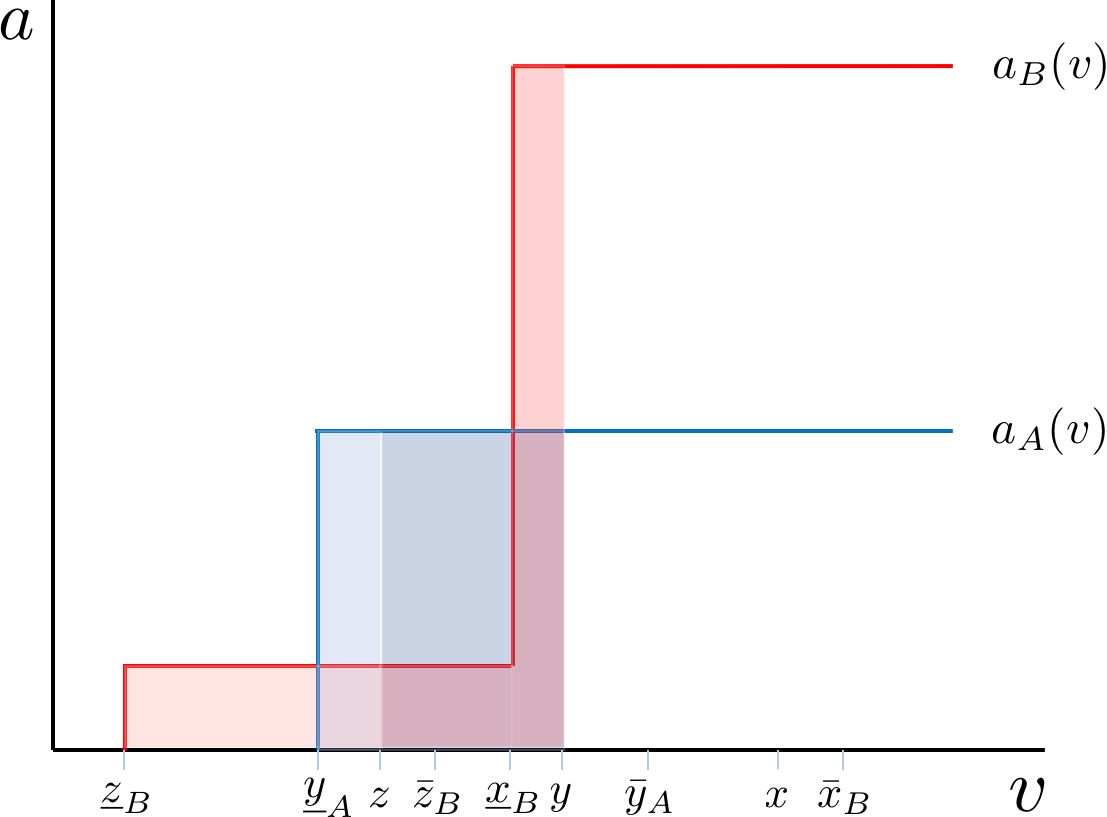
We now show that these sufficient properties hold by induction. As a base case, consider when there is one point in the top chain, which without loss is . By definition of the top chain, and there is flow into item at , which is in ironed interval . We can set and set . Then


For the inductive hypothesis, suppose for any chain of length , we have allocation rules such that (1-5) hold.
Now consider a chain of length . Without loss of generality, let be the top point in the chain, where sits in the ironed interval , and this point is proceeded by which sits in , hence and by definition of the chain.
By the inductive hypothesis, we can come up with allocation rules and that satisfy complementary slackness to the same chain without the highest point , and will have . We construct an allocation rule for the top chain of size as follows; this is depicted in Figure 17. Let . Then let
This clearly satisfies (1-3). To show that (4) holds, we observe that at any previous point of concern , we had . Now at those points, we have . This holds for as well. Thus, complementary slackness is still satisfied at all previous points ; we only need to check equal utility at .
Then to have , since , we require that
The solution here is exactly the defined above.
Alternatively, by replacing with , thus setting , we get a solution that has and as required in (5).
Thus we have ensured that for top chains of all lengths, we can give an allocation rule that satisfies complementary slackness for all values from the bottom to the top of the chain. For below the chain, , so we automatically satisfy complementary slackness. Above the chain, if we have used the alternate solution that (5) guarantees exists, we automatically satisfy complementary slackness for . This would only fail if there is flow into item for —that is, if the dual contains a upper swap, but by assumption it does not. Then for any dual solution with no double swaps or upper swaps, this algorithm gives an allocation rule that satisfies complementary slackness.
We prove that the menu complexity of the mechanism output by this algorithm is finite below:
Claim.
The menu complexity is always finite.
Proof.
Proof by contradiction. Suppose that there exists an instance such that the mechanism output by the algorithm has infinite menu complexity.
Note that this can only happen if the length of the top chain is infinity. Thus, there exists a sequence of points such that the point is inside an ironed interval and . Analogous claims hold for an element in the chain.
Thus, we have
Since the infinite sequence is monotone and bounded, it converges to a limit, say . Observe that satisfies and is unironed. This is because points arbitrarily close to it are unironed and are zeroes of and . However, in this case, our algorithm just sets the price and thus has constant menu complexity, a contradiction.
∎
∎


Appendix G Equivalence with Single-Minded Valuations
In the introduction, we note the following observation.
Observation 2.
The partially-ordered setting is equivalent to the single-minded setting.
First, we define the single-minded setting.
Definition 11.
In a single-minded setting, a seller determines how to sell any bundle of items. A buyer has a (value, bundle) pair where is any subset of items. The pair is drawn from a joint probability distribution over where is the maximum possible value of any bidder for any item.
Any single-minded setting can be represented as a partially-ordered setting: the set of possible interests is just the set of possible bundles, . The relation is set containment: an interest dominates an interest , that is, , if . The distribution is identical.
Any partially-ordered setting can be represented as a single-minded setting: we can invent items such that every interest maps to some subset of items. For any minimal interest (that is, which does not dominate any other interests), map to a new item : . For each successive interest , map to where is a new additional item. Repeat this process, completing a mapping from interests to subsets of some created items. For all subsets which do not have an interest that maps onto it, assign measure to the event of drawing from . Otherwise, .
Appendix H The Master Theorem
All of the analysis in the previous section started from a candidate dual solution, and showed that such duals are optimal (as in, there is a feasible primal satisfying complementary slackness). The missing step is ensuring that there exists an input distribution for which these duals are feasible. To save ourselves (and future work) the tedium of hand-crafting an actual distribution for which these duals are feasible, we prove a general Master Theorem, essentially stating that for a wide class of duals (essentially, anything dictated by ironed intervals, positive/negative regions, and flow in), there exists a distribution for which this dual is feasible.
Theorem 9 (Master Theorem).
Suppose we are given a partial order over , for each item candidate endpoints of zero region (bounded away from ) , a finite set of candidate ironed intervals (bounded away from zero) with , and for each pair of items a finite set of candidate flow-exchanging points (bounded away from zero) not in for any candidate ironed interval. Then there exists a joint distribution over (value, interest) pairs with a feasible dual such that:
- •
the endpoints of the zero region for are and .
- •
the ironed intervals of are exactly to the intervals (no others).
- •
for some .
Note that from the proof the Master Theorem, it is clear how to explicitly construct a distribution for the lower bound (although this is a tedious and unilluminating process).
In this section we provide a complete proof of Theorem 9. On our way to prove this theorem, we generalize a result of Saxena et al. 2018, in which they show that for totally ordered preferences, one can always find a discrete distribution that produces a well-enough-behaved revenue curve. They use this result to show that there exist instances for which the menu complexity is the worst possible, exponential in the number of items. Here we extend their construction and show that for any well-enough-behaved set of continuous revenue curves for the partially ordered setting, there exist distributions that induce them.
The first step is to generalize the result of Saxena et al. 2018 from discrete distributions to continuous distributions.
Lemma 7 (Revenue Theorem for Continuous Curves).
Given a continuous curve differentiable everywhere except at countably many points, such that and , there exists a distribution such that is the revenue curve that arises from selling to a single bidder with a valuation drawn from .
Proof.
Consider the following distribution
and for , for . In order to show that this is a valid distribution, it suffices to show that it is monotonic non-decreasing. For that, we consider its derivative and show it is non-negative everywhere:
It suffices to show that the numerator, , is always non-negative. Note that for , (since and the derivative doesn’t change fast enough) and . Since , the claim follows.
It remains to show that indeed the revenue from this distribution matches the curve . Consider setting a price of , then the revenue of selling at is exactly . ∎
Now we want to extend this to say we can find distributions for revenue curves with specific properties that will be useful.
Theorem 10 (Master Theorem for Single Item).
Given candidate endpoints of zero region and candidate ironed interval endpoints (where ) there is a distribution such that the revenue curve induced by a bidder whose valuation is drawn from satisfies
- •
is negative for (i.e. is the lower endpoint of the zero region),
- •
is positive for (i.e. is the upper endpoint of the zero region) and,
- •
the ironed intervals correspond exactly to the intervals for to .
Proof.
We will reduce the problem of finding a valid distribution to that of constructing a revenue curve that will guarantee these properties and then apply Lemma 7. Consider the following revenue curve:
This revenue curve is such that and for . This allows us to claim that there is a distribution that induces this revenue curve. Moreover, from the way we constructed this revenue curve, the derivative is positive from to , negative from to , goes from negative to positive for the intervals and is elsewhere. We will show that these conditions are sufficient to make the virtual values take the signs we intend them to.
It suffices to note that the sign of the derivative of the revenue at is the opposite of the sign of the virtual value at (noted in Definition 1). By construction, our revenue curve has negative slope on values higher than and positive slope on points below . The intervals in between will be ironed and turn into slope intervals. ∎
Remark 4.
It is possible to relax the condition that all ironed intervals are between . It is not hard to see how to adapt the proof to have ironed intervals either in or . It is sufficient to add dimpled intervals, like the ones in our construction, as the revenue curve is increasing or decreasing. We don’t need them for our main result, hence don’t worry about this more general result. Likewise, the revenue curve could be made differentiable everywhere if we used a smoother function to transition between the ironed and non-ironed intervals, as opposed to straight lines.
Proof of Theorem 9.
If the constraint over flows wasn’t there, the problem would be a direct application of Theorem 10. Unfortunately, the flow constraints may affect the virtual values of neighboring items. It is not hard to predict how outgoing and incoming flow will change the virtual values for the different items. From the study of duality in this context we know that if there is -flow leaving from to (where ), then the virtual values of all points of item with will increase by and all points of item with will decrease by . Thus, given that we know what we want the revenue curves to look like after all flow has been sent, we can reverse engineer what they must look like in order to make that happen. In particular, since the flows shift the virtual values by a constant it will suffice to subtract a function whose value is before and becomes a line with small, negative slope at (say, slope ) from the “suggested” (by Theorem 10) revenue curve for item (since these will increase by after the flow is sent) and add positive slope functions of the same value at on item from its suggested revenue curve (since these will decrease by after the flow is sent). This is sufficient because of the connection between virtual values and revenue curves argued before: the derivative corresponds to changes in the virtual value. So for a constant change in virtual value, the matching change would be adding a linear term to the revenue curve of opposite sign. The order in which we do these changes is by processing items from leaves to the root (i.e. only process a node once all its children have been processed) and within an item , address the flow-exchange values from smallest to largest. ∎
We abuse this opportunity to prove a similar result for the multi-unit pricing setting.
Theorem 11 (Master Theorem for MUP).
Suppose we are given a MUP instance where the buyer can get up to copies of an item. Let for be the item corresponding to copies. For each item we are given candidate endpoints of the zero region and a set of candidate ironed interval endpoints with . Moreover, for each tuple and , we are given a set of candidate flow-exchanging points and not in for any candidate ironed interval. Then, there exists distributions for all items such that:
- •
the endpoints of the zero region for correspond to ,
- •
the ironed intervals correspond exactly to the intervals (and no other),
- •
the dual of the problem is such that there (i.e. there is flow sent from at to into and no other flow from to ).
- •
the dual of the problem is such that there (i.e. there is flow sent from at to into and no other flow from to ).
Proof.
This proof is similar to that of 9 with the exception that on the former, increasing the flow from to (with ) by a little bit increases and decreases the virtual values below by the same amount. This is no longer true since we are moving from to . In this case, sending flow from to increases the virtual values below by but decreases the ones on the other end by only . So, in order to reverse engineer the change in virtual value induced by this setting we need to add the same functions as in the proof of Theorem 9 to the revenue curve suggested for and add a -scaled version of it for the receiving item at the point on the revenue curve for . The order in which these we do these changes is by processing items from leaves to root (i.e. from to ) and within a item , address the flow-exchange points from smallest to largest. ∎
Appendix I A Candidate Dual for a Lower Bound on Menu-Complexity for the Multi-Unit Pricing Problem
Consider an MUP instance where the buyer can get one, two, or three copies of a given item. The relevant complementary slackness constraints in this setting go from
- •
Rightwards. For all , from and . This is because a buyer can always misreport and get more items.
- •
Leftwards. For all , from and . This is because a buyer would prefer getting fewer items if they are available for much cheaper.
As shown in [9], a buyer of type ’s utility for reporting is given by . The same buyer’s utility for reporting is given by .
To construct a lower bound for the MUP instance, we adapt our construction from the partially ordered case. We describe our construction formally below, but note here all the relevant differences. Observe that the incentive compatibility constraints for the MUP instance described above hide a partially ordered instance inside them. Indeed, the ‘item’ is analogous to the item , while the items and are the items and respectively. Just like the partially ordered instance, there are incentive compatibility constraints from for all . The only difference is that the constraints from have been replaced by those from . Also, there are ‘new’ constraints from and .
We claim that, despite these changes, the essence of our argument there still holds. Roughly speaking, our argument there involved constructing a top-chain (see Definition 7) oscillating between items and . For any value in this chain, we had flow coming from to both and . Reasoning about complementary slackness constraints, then, gave us our lower bound.
For the MUP case, we can still do all the above things with the caveat that the value has to be treated as if it were . An analogous master theorem can still be proved as the effect of the ‘diagonal’ flow on the virtual values is predictable. Using the master theorem, we can construct (essentially) any dual we want. Thus, we can have a feasible dual with a top-chain of an arbitrary length oscillating between items and . Also, we have flow from the item to both and at all values in this top-chain. Chasing through the complementary slackness constraints in this dual again gives us a lower bound.
To highlight this analogy, in what follows, we use instead of , instead of , and instead of .
Formally, we construct given an integer , a dual containing a top chain among and of length . That is, a sequence of points such that
In this dual, we have no extra space between the ironed intervals:
- •
/2, , and for such that and are in the chain, .
- •
, , and for such that and are in the chain, .
Recall that by definition of the and operators, is ironed in . Also by our definitions, for ; for ; for .
We will also define to be DMR (and thus have no ironed intervals) with and .
We adapt the flow from the partially ordered lower bound example: for any in the chain, and .
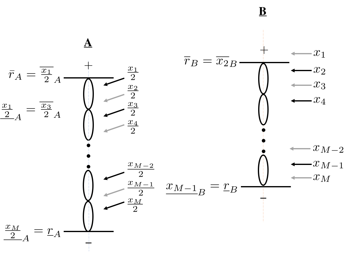
Theorem 12.
To satisfy complementary slackness with the candidate dual, the allocation requires distinct allocation probabilities; the menu complexity is at least .
Proof.
The proof is almost identical to that of Theorem 1. Using the constraint that the allocation can’t increase in the middle of an ironed interval and that for all in the chain, we show that the allocations must be non-zero throughout the chain.
Then, we show that for consecutive points in a chain that , and similarly, for , that
This is enough to show that all of the menu options must be distinct, requiring meu complexity . ∎
Appendix J Coordinated Valuations
In this section and the following Appendix K, we examine the same minimal partial ordering with where . However, a type now has a function and describe his valuations for and respectively, and . That is, if a buyer with type gets item , his utility is times the probability that he is served minus his payment.
The main result is that even for that is piecewise linear with only two segments and for , the randomization required in the optimal mechanism jumps from unbounded but finite, as it was in the partially-ordered setting, to countably infinite. This further fills out the spectrum, placing this setting between partially-ordered items and two additive items.
However, if and are not piecewise linear, the menu complexity once again jumps up, becoming uncountably infinite, and matching the menu complexity for two additive items.
J.1 Preliminaries
Consider selling items , , and to one bidder. Define the set . We use to refer to a general item . When we make claims about , we mean that the claim holds for each of the three items in . When referring only to items , , we use the symbol . Thus, a claim that holds for holds for both and .
In the setting we consider, the bidder has a type in the set , where is some constant. The type of the bidder is drawn from a distribution supported on . Denote by . Also, define as the distribution conditioned on . Almost exclusively, we refer to as . We also omit the subscript when it is clear from context.
We now define the bidder’s value function . This is defined as
where is an increasing, invertible function that is Lipschitz with parameter and for all . Intuitively, this means that if the bidder has type , then their value for item is . A bidder with type has the value for any item and value for the item .
Mechanisms.
A mechanism is defined by two functions , , where and . The function is called the allocation rule and the function is called the payment rule. We will use to denote and to denote . A mechanism is said to be incentive compatible if, for all
| (21) |
Instance.
An instance for the coordinated items setting is defined by a tuple . We will usually omit the subscript and simply write . Our goal is find, for a given instance , the incentive compatible mechanism that maximizes the revenue .
J.1.1 A Linear Programming Formulation
For an instance for the coordinated items , finding the incentive compatible mechanism that maximizes turns out to be equivalent to the linear program in Equation 22. Here and throughout, for a distribution supported on , we use to denote the Myerson’s virtual value function, where is the cumulative distribution function for the distribution defined by .
| maximize | (22a) | |||||
| subject to | ||||||
| (22b) | ||||||
| (22c) | ||||||
| (22d) | ||||||
| (22e) | ||||||
Even though the argument that Equation 22 is equivalent to finding the incentive compatible mechanism that maximizes is standard, we summarize it here. Observe that the non-trivial incentive compatibility constraints in Equation 21 can be classified into two types:
- •
and : In this case, Equation 21 reduces to . This is attainable for all , if and only if the allocation rule is monotone increasing (Equation 22c) and .
- •
and : In this case, Equation 21 reduces to . Due to the constraints in the previous paragraph, it is sufficient to have . This is equivalent to the constraint in Equation 22b.
Finally, it can be verified that if , then .
We will use to denote a general solution to Equation 22 and to denote the optimal value for the instance .
J.1.2 A Lagrangian Dual Formulation
For any instance of coordinated items , the revenue maximization problem is defined in Equation 22. Let be a discrete set of points in . Define the -dual of Equation 22 as:
| minimize | (23a) | |||||
| subject to | ||||||
| (23b) | ||||||
| (23c) | ||||||
where
Equation 23is obtained from Equation 22 by Lagrangifying the constraints Equation 22c using the variables , the constraints Equation 22b using the variables , and the constraints Equation 22b, for using the variables . Here and throughout this paper, we define and for notational ease. We note that getting Equation 23 from Equation 22 requires integrating a certain term by parts. Throughout this work, we assume that our functions are well-behaved enough to allow such standard operations.
Note that the idea of using a Lagrangian dual is not new to this work. Indeed, a lot of recent advances in similar settings have been made using this technique. We will use to denote a general solution to Equation 23 and to denote the optimal value for the instance . Often, we will abbreviate to or even if the subscript and superscript are clear from the context.
We have the following ‘strong duality’ result (proof in Appendix K.1):
Theorem 13 (Strong Duality).
Let be an instance of coordinated items .
- (a)
Let be a discrete set. For any feasible solution of Equation 22 and any feasible solution of the -dual (Equation 23), it holds that:
Equality holds if and only if the following conditions are satisfied almost everywhere:
(24a) (24b) (24c) (24d) (24e) - (b)
There exists a set such that .
The main reason we provide a proof for this ‘strong duality’ result is that the variables are parametrized by a continuous variable. We could not find any results for such variables that subsume our setting. Our proof of Theorem 13 works by showing, for all , a discrete linear program that has almost the same primal and dual value (up to terms depending on ). Since strong duality holds for discrete systems, this gives us that the duality gap of our linear program is small. Theorem 13 then follows as the feasible region is closed.
J.1.3 Our Framework
Fix an instance and discrete set .
The Dual Framework.
Let be a feasible solution for the -dual, i.e., Equation 23. Define
If the (resp. ) is over an empty set, we define it to be (resp. ).
We sometimes refer to and as representing flow, e.g., we say that there is flow from to if or .
An interval is said to be ironed on a item if and for all , we have .
The Primal Framework.
Let be a feasible primal solution for Equation 22. Let be an interval. Define to be the number of distinct values taken by the function over the interval . Also, define . We omit the argument if it is .
We define the menu complexity of the instance , to be the smallest menu complexity of any optimal solution to Equation 22.
J.1.4 Formal Statements of our Results
Theorem 14.
There exists an instance of coordinated items such that is uncountably infinite. Furthermore, the instance satisfies and all the distributions are DMR1515 15 Recall that a distribution is DMR if the Myerson’s virtual value function is non-decreasing..
Theorem 15.
For any instance such that the functions are piecewise linear, we have is at most countably infinite.
Theorem 16.
There exists an instance of coordinated items such that is countably infinite. Furthermore, the instance satisfies and all the distributions are DMR, and the function is piecewise linear.
Theorem 17.
There exists an instance of coordinated items such that is countably infinite. Furthermore, the instance satisfies and the function is piecewise linear with only segments.
J.2 Master Theorem
For our lower bounds, we will construct instances that have a large menu complexity. To show a lower bound on the menu complexity, we will define a feasible solution to the -dual (Equation 23), for some , show that it is optimal, and then show that any feasible primal that satisfies complementary slackness (Equation 24) with this dual must have a large menu complexity. Below, we prove a ‘Master Theorem’ (Theorem 18) (proof in Appendix K.2) that constructs instances together with a feasible dual solution with some desirable properties.
Theorem 18 (Master Theorem).
Let be fixed. Suppose that, for all , points are given. Let , be discrete subsets of . Consider finite or infinite sequences of disjoint intervals
where and . Then, for any invertible functions , there exists an instance and an -dual such that the following hold:
- •
for all .
- •
The value of is non-decreasing and and .
- •
throughout and for some .
- •
for some .
- •
for some .
Moreover, if is empty, then the distributions are DMR.
J.3 Lower Bounds
J.3.1 DMR Distributions
Let be a non-decreasing function that is continuous except at countably many points. In this subsection, we construct an instance of coordinated items such any optimal solution of Equation 22 for satisfies that 1616 16 We abuse notation slightly here. What is meant is that takes the same values over the interval as takes over the interval (see subsubsection J.3.1 for the exact statement).. In our construction, the distributions are DMR and .
Two important instantiations of this general procedure prove Theorem 14 and Theorem 16. For Theorem 14, we construct by setting need . For Theorem 16, we construct by setting to be a function that takes countably many values. A concrete example of such a function is one that has countably many “steps” as it moves from to . We take care that the function is piecewise linear in .
The Instance
For notational convenience, we work in the range in this subsubsection. Consider an increasing function and let . Let . Note that is well defined for and define:
It is readily seen seen that satisfies in the interval . Let and apply Theorem 18 with and
- •
, , , , .
- •
are empty
- •
.
This gives an instance and an -dual solution such that the distributions are DMR and :
- •
For all , and and .
- •
are throughout.
- •
.
The Analysis
Recall , , and constructed above. Define a feasible primal solution of Equation 22 for as:
In Lemma 8 (proof in Appendix K.3), we show that and satisfy complementary slackness. To finish our menu complexity lower bound, we argue that any primal that satisfies complementary slackness with must have . This proof is in Lemma 9.
Together with strong duality (Theorem 13), Lemma 8 shows that is optimal. Thus, any optimal primal for must satisfy complementary slackness with . Lemma 9 says that for this primal and thus, it has a high menu complexity.
Lemma 8.
The primal is feasible and , satisfy complementary slackness (Equation 24).
Lemma 9.
Consider any feasible primal that satisfies complementary slackness with must , where is the allocation for item in .
Proof.
We reason from Equation 24. Specifically, the constraints (24a), (24b) for item imply that for and for . Thus, we have:
Since for all , we have by (24d) that for all in this range. Thus, for all :
Since the right hand side in the equation above is independent of the primal, we get for all that . Thus, for all , we have implying in this range. The constraints (24a), (24b) for item fix the allocation outside . Combining, we get that .
∎
J.3.2 Proof of Theorem 17
In the last subsection, we showed that instances can have high menu complexity, even when all the distributions are DMR. The reason for high menu complexity is the complexity in the functions . We now show that if the distributions are not required to be DMR, even ‘simple’ (e.g., piecewise linear with only segments) functions can have countably infinite menu complexity. Two segments are required because of the arguments in Appendix F. This is tight due to our upper bounds in subsection J.4.
The Instance
For notational convenience, we work in the range in this subsubsection. Define:
We define points , , and , for . Note that the sequence converges to .
In order to construct , we apply Theorem 18 with and
- •
, , , , , .
- •
for some . for some .
- •
is empty and .
This gives an instance and an -dual solution such that :
- •
For all , and and .
- •
are throughout. if and only if for some and if and only if for some .
- •
.
The Analysis
Recall the definitions of and the instance above. Define a feasible primal solution of Equation 22 for as:
We proceed exactly as in subsubsection J.3.1. In Lemma 10 (proof in Appendix K.4), we show that and satisfy complementary slackness. To finish our menu complexity lower bound, we argue that any primal that satisfies complementary slackness with must have infinite menu complexity.
Together with strong duality (Theorem 13), Lemma 10 shows that is optimal. Thus, any optimal primal for must satisfy complementary slackness with . Lemma 11 says that such a primal has infinite menu complexity
Lemma 10.
There primal is feasible for and , satisfy complementary slackness.
Lemma 11.
Any feasible primal for with a finite menu complexity does not satisfy complementary slackness with .
Proof.
Proof by contradiction. Let be a feasible primal with finite menu complexity that satisfies complementary slackness with .
Let be the largest such that or . If no such exists, we define . Since is assumed to be finite and the allocation is monotone (by constraint (22c)), is well defined and and is constant for all . Let the constant values be and respectively.
Since , satisfy Equation 24, we have, by Equation 24c
| (25) |
Also, for all we have by the constraint (24e) (applied once to both and )
| (26) |
We derive a contradiction in two steps. First, we prove
Claim.
.
Proof.
Claim.
.
Proof.
Proof by contradiction. Suppose that . By Equation 24a, we have for all . Since are in the same ironed interval on and are in the same ironed interval on , we have using Equation 26 that
Plugging in the values of , we have
a contradiction to . ∎
These two claims together with Equation 25 establish that . We now give a contradiction assuming is even. A similar argument works if is odd. Since lie in the same ironed interval in , we have . By choice of , we have . By Equation 26, we have
a contradiction to Claim . ∎
J.4 Upper bounds
In this subsection, we prove that for any instance such that the functions and are piecewise linear, we have is at most countably infinite (Theorem 15). This result is tight by our arguments in subsection J.3
Our line of argument is as follows: Fix an instance . By Theorem 13, there exists an , a primal solution and an -dual solution that satisfy complementary slackness. From , we construct another primal solution such that is small and , satisfy complementary slackness. Thus, the primal also defines an optimal revenue mechanism. The menu complexity of this new mechanism gives us our upper bound on .
We note that this technique is markedly different from that employed in Appendix F where we assume an optimal dual and describe a recovery algorithm that reads an optimal primal from the optimal dual. Here, we assume both, an optimal dual and an optimal primal1818 18 Note that we need Theorem 13 to assume that there exists an optimal primal-dual pair that satisfies complementary slackness., and prove that such a primal can be improved to have a lower menu complexity.
J.4.1 Splitting
Our procedure to improve the primal makes extensive use of the following “splitting” operation:
Definition 12.
Let be a function and consider the interval , where . Define the function as :
The following is easily observed for all :
| (27) |
If and are two disjoint intervals, then . We will use to denote this common value.
Remark 5.
Let be a function and be an interval. For any , we have
Lemma 12.
Let be an increasing function and be an interval. We have . Moreover, equality holds if or is constant over the interval .
Proof.
Let . Since is increasing, we have
Rearranging gives the result. The moreover part can be using Equation 27 and Definition 12. ∎
J.4.2 Proof of Theorem 15
Fix an instance and let , be an optimal primal dual pair ( is -dual for some ). Without loss of generality, we can assume that the product is non-decreasing (see Appendix A). We define the function to be if , if , and if . Using , define the following notion of a strip.
Definition 13 (Strip).
A strip is an interval , where , such that the following hold:
- •
For all , there functions are linear over
- •
For all , the function is constant for .
- •
For all , the function is constant for .
The following holds for any strip.
Lemma 13.
For as above, let be any strip. There exists another primal solution of such that
- •
for all .
- •
, satisfy complementary slackness (Equation 24).
- •
For all , it holds that .
The proof of this lemma spans the rest of this subsection.
Proof.
Let . Define the function 1919 19 Note that this is just the utility of a bidder with type .. Since the functions are continuous, and is continuous except at countably many points, we have that is also continuous. Define points , as follows2020 20 Throughout this subsection, we define several infimums and supremums. In case the argument to any of these is empty, we simply drop those terms from where they are used. For example, if , are not defined, we simply use instead of below.:
We use and to define:
Now, define:
Finally, we define:
Our primal is defined by the allocations . Note that item and item are straightforward from Definition 12. We only concentrate on item .
For item , we verify each of the constraints in Equation 24. For Equation 24a, observe that if for some and some , then, since is a strip, throughout . Thus, the allocation is throughout and our operations have no effect. If , then the result follows as , satisfied complementary slackness. A similar argument verifies Equation 24b and Equation 24c.
For Equation 24d, consider a such that . If , then the result follows because of Remark 5 and the fact that satisfy complementary slackness. If , then, since satisfied complementary slackness, we have . Thus, by Lemma 12, implying that . Suppose that . The other cases are similar. We have:
| (Remark 5) | ||||
| ( over a strip) | ||||
| (Definition of , ) | ||||
| (Remark 5) |
Equation 24eis verified similarly.
∎
Proof of Theorem 15.
Since the functions are assumed to be piecewise linear, we can partition the range into countably many disjoint strips. Theorem 15 follows by applying Lemma 13 to each of the strips. ∎
Appendix K Missing Proofs From Appendix J
K.1 The Proof of Theorem 13
K.1.1 The Proof of item (a)
Proof.
Fix . Observe that :
Using the definition of , we get
First, note that, integrating by parts, we have by Equation 22c. Fix any . Grouping all the terms with , we observe that is multiplied by by Equation 22b. Similarly, fix any . Grouping all the terms with , we observe that is multiplied by by Equation 22b.
Thus, we have . To finish the proof, observe that the conditions in Equation 24 are exactly those needed to make these inequalities tight. ∎
K.1.2 The Proof of item (b)
Proof.
We prove that for all , there is a set such that . The statement then follows because the the union of the region in Equation 23 for all possible sets is closed. Recall that the functions are -Lipschitz.
Fix and let be sufficiently small. Our proof proceeds by defining a discrete linear program (Equation 28) and its dual (Equation 29) for . Let the optimal value of Equation 28 be and the optimal value of Equation 29 be . Since strong duality holds for discrete linear programs, we have . We also ensure that for all .
In Theorem 19, we show that . In Theorem 20, we show that there is a set such that . Combining, we get
for small enough . ∎
The rest of this subsection is devoted to defining and analyzing the discrete linear program, in order to prove Theorem 19 and Theorem 20.
K.1.3 The Discrete Linear Program
We describe a discrete linear program for the instance . The instance is fixed for the rest of this subsection. Without loss of generality, let be such that is an integer.
The Primal
Consider the following optimization problem with the variables and for . In this subsection, we abuse notation and write instead of . Define and .
| maximize | (28a) | |||||
| subject to | ||||||
| (28b) | ||||||
| (28c) | ||||||
| (28d) | ||||||
| (28e) | ||||||
| (28f) | ||||||
It is easy to see why . We also have:
Theorem 19.
The optimal value of Equation 28 satisfies .
Proof.
Let and be the optimal solution for Equation 28. Consider the set . Using the set , we now define a mechanism for the continuous revenue optimization problem. Consider a type . Define:
Let be the mechanism that allocates item with probability and charges price to a bidder who reports 2121 21 We slightly deviate from our definition of a mechanism and allow to be different from .. Observe that is a truthful mechanism. By a standard argument, there exists a feasible solution to Equation 22 such that is the expected revenue of . We now prove that .
Couple a bidder in with (continuous) type with a bidder with (discrete) type where is the smallest value such that . The coupling is valid as . We show that . Taking the expectation on both sides gives the result.
Observe that:
Adding, we get that
Since , we have
| () | ||||
| ( is -Lipschitz) |
∎
The Dual
Consider the following Lagrangian relaxation of Equation 28, where we Lagrangify the constraints Equation 28b using the variables , the constraints Equation 28c using the variables , and the constraints Equation 28d using the variables . We use the convention that
| minimize | (29a) | |||||
| subject to | ||||||
| (29b) | ||||||
| (29c) | ||||||
| (29d) | ||||||
where terms like are defined to be and
Theorem 20.
The optimal value of Equation 29 satisfies where .
Proof.
We proceed by defining a feasible solution of Equation 23 from the optimal solution of Equation 29 with the same value. Throughout this proof, we denote the variables of the discrete linear program using a ‘hat’. Let be the optimal solution to Equation 29. Define . Define an -dual solution for as follows
where is the largest integer such that . Observe that is feasible and
Since is constant in , we have:
K.2 Proof of Theorem 18
We need the following technical lemma:
Lemma 14.
Let and be a function such that and for all such that , we have . Then, there exists a distribution supported on such that
Proof.
Define:
Observe that satisfies the requirements of the theorem. To prove that is a valid distribution, it is sufficient to show for all . We first note that . Thus, the only case left is when . In this case,
∎
Proof of Theorem 18.
Let be such that and for all . In order to define , define
Let throughout. Also, define:
Finally, define and and ,
Observe that the function satisfies all the requirements of Lemma 14. Thus, there exist distributions such that
Set , and to be the unique function such that .
Observe that the dual defined by satisfies all the requirements of the theorem.
∎
K.3 Omitted Proofs in subsubsection J.3.1
Proof of Lemma 8.
We verify each of the constraints in Equation 24 and leave verifying feasibility using Equation 22 to the reader. The constraints (24a), (24b) are verified easily. The constraint (24c) is true because throughout. The constraint (24d) holds because for all , we have
and the three quantities are equal. Finally, the constraint (24e) is satisfied because is zero throughout.
∎
K.4 Omitted Proofs in subsubsection J.3.2
Recall that , , and , for . This implies the equations
| (30a) | ||||
| (30b) | ||||
| (30c) | ||||
| (30d) | ||||
We will need the following lemma:
Lemma 15.
For all and ,
Moreover, equality holds if .
Proof.
We calculate the three quantities:
We now prove the result for . In this case, as the expressions for and are the same, it is sufficient to show that
| (Equation 30d) | ||||
| (As ) |
We now prove for even . The case for odd is similar. Note that and for all . In this case, as the expressions for and are the same, it is sufficient to show that
| (Equation 30c) | ||||
| (As ) |
The moreover part can be observed by putting in our equations. ∎
Proof of Lemma 10.
Feasibility
We verify the feasibility constraints in Equation 22. It is straightforward to verify that are monotone (constraint (22c)) and take values in (constraint (22d)). Finally, the constraint (22b) holds because of Lemma 15.
Optimality
We verify all the constraints in Equation 24. The constraints (24a), (24b) are straightforward to verify from the definition of . The constraint (24c) follows from the fact that is throughout and
The constraint (24d) holds because is throughout. For the constraint (24e), we need to prove that for all
which holds because of (the moreover part of) Lemma 15
∎