When to Limit Market Entry under Mandatory Purchase
Abstract
We study a problem inspired by regulated health insurance markets, such as those created by the government in the Affordable Care Act Exchanges or by employers when they contract with private insurers to provide plans for their employees. The market regulator can choose to do nothing, running a Free Market, or can exercise her regulatory power by limiting the entry of providers (decreasing consumer welfare by limiting options, but also decreasing revenue via enhanced competition). We investigate whether limiting entry increases or decreases the utility (welfare minus revenue) of the consumers who purchase from the providers, specifically in settings where the outside option of “purchasing nothing” is prohibitively undesirable.
We focus primarily on the case where providers are symmetric. We propose a sufficient condition on the distribution of consumer values for (a) a unique symmetric equilibrium to exist in both markets and (b) utility to be higher with limited entry. (We also establish that these conclusions do not necessarily hold for all distributions, and therefore some condition is necessary.) Our techniques are primarily based on tools from revenue maximization, and in particular Myerson’s virtual value theory. We also consider extensions to settings where providers have identical costs for providing plans, and to two providers with an asymmetric distribution.
1 Introduction
In the Affordable Care Act (ACA) Exchanges, the government plays the role of the market regulator, contracting with several private health insurance providers to offer insurance plans to a number of patients, or consumers. Each insurance provider posts a price for his insurance plan, which he can sell to an unlimited number of consumers, and then each consumer chooses a plan to purchase among those for sale. Further, the ACA originally imposed an “individual mandate” that charges a steep penalty to consumers who do not purchase any plan, whose aim was to essentially make it mandatory for every consumer to purchase some plan.
In the ACA exchanges, prices set by providers tend to be high11 1 In 2013, even with subsidies, premiums represented between 4 and 9.5% of the median income [Johnson et al. 2013]. In 2015, a survey found that without subsidies, average marketplace unsubsidized premiums were over what most consumers claim is the maximum they can afford [Williams 2016]., and little regulatory power exercised is by the government (for example, the ACA establishes minimum coverage guarantees, but otherwise is not an active regulator). One reason cited for these high prices is that the insurance market has a high barrier to entry, so once incumbent providers have surpassed this barrier, they face little competition. The motivating scenario to have in mind is that there may be multiple incumbents but, due to entry barriers, each incumbent serves a section of the market significantly better than all others. Could the government improve consumer utility by further regulating the market? For instance, what if the government were to only allow the insurance providers offering the five least expensive plans to enter the exchanges? This would create competition and ensure lower prices. However, it would also mean fewer options, excluding the favorite choices of some consumers’ from the market, and thus leading to lower consumer welfare. That is, such regulation decreases both prices and welfare, so it not immediately obvious whether it improves consumer utility (which is the difference of the two). The main purpose of this paper is to provide theoretical tools to reason about this tradeoff, and understand under what circumstances consumer utility is improved.
The ACA exchanges are an example of a regulated health insurance market. Another common example concerns an employer who contracts with providers in order to provide health insurance to her employees. In this paper, we focus on such regulated markets, where a market regulator can determine which providers enter the market, and where every consumer must purchase a plan.22 2 Put another way, the outside option of purchasing nothing is so undesirable that all rational consumers will choose to purchase something, even at negative utility. This may be due to an explicit fine (individual mandate), or simply because the outside option of being uninsured is so undesirable. But we do not explicitly model this undesirable outside option. Note that while healthcare is our motivating example, the model is not limited to only healthcare, but applies to any situation where purchase is mandatory.
The focus of this paper is the following: under what conditions does limited entry (reducing prices via competition, but also reducing welfare via reduced options) improve consumer utility?
Observe that reasoning about this question requires a direct understanding of what prices the providers will choose to set. As such, our main techniques involve characterizing and analyzing equilibria, and understanding when they exist and are unique. We compare two settings: the Free Market setting, where the market regulator does not restrict entry at all, and the Limited Entry setting. Note, of course, that while we use healthcare exchanges as a motivating example, the focus of our paper is to provide a model and theoretical tools which are generally applicable. As such, our model is stylized and intended to capture one key decision facing regulators of healthcare exchanges (whether to limit entry or not)—it is not intended to capture verbatim the full range of challenges facing healthcare regulators. Still, we do emphasize that this is indeed a key decision facing regulators of healthcare exchanges, and that theoretical tools from mechanism design indeed provide insight to make these decisions.
1.1 Model and Results
Our goal is to provide a clean model to reason about the impact of limiting entry. To this end, we consider providers, and consider a population of consumers, each with a value for the plan offered by provider . For the majority of the paper, we consider the symmetric setting, where a random consumer from has value for plan drawn i.i.d. from some single-variate distribution (that is, while individual consumers have different values for different providers, the providers are a priori identical).33 3 To have an example in mind, consider a provider which offers a good network for patients with diabetes, and another which offers a good network for patients with a history of cancer. Any particular patient will of course have different values for the plans, based on their own medical history. But the population as a whole does not necessarily prefer one over the other. We denote this as .
In Section 3, we study the Free Market setting, where each provider simply sets a price , and consumers drawn from purchase the plan which maximizes their utility . We first identify sufficient conditions on (involving a new condition we term “”) for the existence of a unique symmetric equilibrium, and we characterize the equilibrium prices in the Free Market. Here, denotes the expected hazard rate of the second-highest of i.i.d. draws from , and formal definitions of both technical terms appear in Section 2.
Theorem 1.1.
Let , where is and has decreasing density. Then the unique symmetric equilibrium in the Free Market setting is for each provider to set price .
Observe that a characterization of a canonical equilibrium in the Free Market setting is necessary if we are to possibly anlayze consumer utility. We include one vignette regarding our technical approach, which leverages machinery from the revenue maximization literature Myerson 1981. Suppose all other providers are setting price ; what is a provider’s best-response? To reason about this, consider instead a new distribution such that is the probability that a consumer drawn from marginal will purchase from this provider if he sets price , given that all other providers set price . The provider’s best response is to set which maximizes his expected profit, , and is therefore a symmetric equilibrium if and only if . Using this rephrasing, we then argue that if this distribution happens to have a monotone hazard rate (MHR), then we are guaranteed the existence of a unique equilibrium. Of course, this distribution is quite different from itself (for example, may be MHR and may not even be regular!). We define a new distributional assumption, , such that if is then this implies that is MHR. We postpone a formal definition of to Section 3, but only note here that it is a strictly stronger condition than MHR, and that most common MHR distributions are also (e.g. exponential, uniform, Gaussian).
Next, in Section 4, we study the Limited Entry setting. Formally, each provider still sets a price , but now only the providers with lowest price enter the market (tie-breaking arbitrarily). Consumers again pick the plan maximizing , but only among these providers. For symmetric instances, quickly observe that there is a unique symmetric equilibrium, and in it all providers set (so in some sense, our model can be seen as “optimistic” towards the benefits of limiting entry). The main result of this section is a characterization of the precise condition on that implies that consumer utility in the Limited Entry setting will be greater than in the Free Market setting; we call this the Limit-Entry condition.
Definition 1.1 (Limit-Entry Condition).
We say that a symmetric distribution satisfies the Limit-Entry Condition if . Here, is the expected inverse hazard rate of the highest of i.i.d. draws from . (Recall that is the expected hazard rate of the second-highest of i.i.d. draws from .)
Theorem 1.2.
Let and admit a symmetric equilibrium in the Free Market setting. Then the expected consumer utility at the unique symmetric equilibrium in the Limited Entry setting exceeds that at the unique symmetric equilibrium in the Free Market setting if and only if satisfies the Limit-Entry Condition.
Finally, while the Limit-Entry condition is relatively clean, it is not obvious how it relates to more common distributional assumptions. Our final main result shows that the Limit-Entry condition is satisfied under standard distributional assumptions.
Theorem 1.3.
Let , where is MHR and has decreasing density. Then satisfies the Limit-Entry Condition.
Corollary 1.4.
Let , where is and has decreasing density. Then has a unique symmetric equilibrium in the Free Market setting, and the expected consumer utility at this unique equilibrium is exceeded by the expected consumer utility in the Limited Entry setting.
In the interest of completeness, we examine whether any of our assumptions can possibly be relaxed to more standard assumptions (e.g. to MHR). In short, Proposition 1.5 establishes that the answer is no, suggesting that there is indeed a relevant aspect of our stronger assumptions as it relates to our conclusions.
Proposition 1.5.
(Different) distributions with the following properties all exist:
- •
is MHR, but there exists a for which is not MHR (in fact, it is anti-MHR).
- •
is MHR, but has no symmetric equilibrium in the Free Market setting.
- •
has a symmetric equilibrium in the Free Market setting, but does not satisfy the Limit-Entry Condition.
- •
satisfies the Limit-Entry Condition, but does not have a symmetric equilibrium in the Free Market setting.
Finally, we include some extensions. In Section 5, we extend our results to the setting where providers have identical costs for providing service. In Section 6, we consider the case of asymmetric distributions . We prove that if is , then the asymmetric analog, , is MHR. We also show that for two providers, when is MHR, an equilibrium exists.
1.2 Related Work
In order to compare with the literature on procurement auctions, we will call the providers “suppliers.” To the best of our knowledge, this is the first work to study procurement of suppliers under mandatory purchase of consumers. The following literature review pertains to procurement auctions without mandatory purchase for consumers. The most relevant work is that of [Saban and Weintraub 2019]. They also study procurement auctions with heterogenous goods, each owned by a different supplier, a consumer population, and a mechanism designer whose objective is to maximize consumer utility. The simplest comparison between these works is that [Saban and Weintraub 2019] study a wide variety of different procurement models, whereas we focus on depth of one particular model. For example, our work fits into their “First-Price Auction” model (which is only one of many models they consider). But within this model, they consider only a two-supplier setting in a simple Hotelling game [Hotelling 1929],44 4 Specifically: consumers are uniformly distributed along the unit line. Each supplier offers an item with fixed value at the endpoint of the line, and consumers value the items at their value minus the distance. whereas we study this model in significantly more depth and generality.
Other work in procurement [Anton and Gertler 2004; McGuire and Riordan 1995] also studies optimal centralized allocations for consumer utility, where the designer can choose which suppliers allocate to which consumers. We do not study this form of allocation at all.
Most prior work studies the two-supplier case without mandatory purchase. [Engel et al. 2002] also uses a third-party mechanism designer apart from consumers and suppliers, but studies different objectives than us: (1) welfare (consumer utility plus supplier revenue) and (2) supplier revenue minimization. They do not, however, study consumer utility maximization.
Other works allow the consumers to act as the auctioneer [Chen and Li 2013; Dana Jr 2012] and investigate whether it is better for the consumers to have one or two suppliers; the answer differs depending on whether the consumers’ information is private or not. These papers do not have a mechanism designer acting separately from the consumers; they also only study the stylized Hotelling model.
1.3 Brief Summary
We study consumer utility in a market with providers under mandatory purchase, motivated by the current state of ACA exchanges (Free Market) versus employer insurance markets (Limited Entry). We find clean sufficient conditions for equilibria to exist (Theorem 1.1) in the Free Market setting, and establish that conditions like these are also necessary (Proposition 1.5). We also establish clean necessary and sufficient conditions for consumer utility to improve with Limited Entry over the Free Market (Theorems 1.2 and 1.3, and Corollary 1.4).
We also wish to briefly note the technical highlights. Typically, establishing existence/uniqueness of market equilibria requires solving a system of non-linear equations (and establishing uniqueness). Of course, our proofs must also accomplish this, but we get a surprising amount of leverage via Myersonian virtual value theory. That is, we interpret equilibrium conditions as one price being revenue-maximizing for a related consumer distribution. Due to mandatory purchase, this interpretation (while mathematically involved) is conceptually fairly clean. This enables us to break down a complex mathematical proof into conceptually digestible chunks, and also provides insight into the right conditions to search for. We are optimistic that these tools will continue to be useful in extensions beyond those considered explictly in this paper.
2 Notation and Preliminaries
We consider the following problem from the perspective of a market regulator. We use the language of healthcare providers throughout the paper (although we again remind the reader that healthcare exchanges are just a motivating example for our stylized model). There are providers, each of whom produces a single (distinct) plan. Each individual consumer in the market has a valuation vector for the plans, with denoting their value for plan . The market consists of a continuum over valuations , which can alternatively be interpreted as a distribution (over a random consumer drawn from the market).
We assume throughout the paper that is a product distribution (that is, for single-dimensional ). We will use to denote the CDF of , and assume that each also has a density function, or PDF, denoted by . For our main results, we will also assume that is symmetric (that is, for all , or the valuations are identically drawn across providers). In Section 6, we consider extensions to asymmetric distributions.
In our context, let’s briefly elaborate on these assumptions. Assuming that each admits a density function is extremely common in past literature (e.g. Myerson 1981), and is comparable to a “large market” assumption that no particular individual has an oversized role. The motivation for this assumption is purely technical, since it allows for clean closed-form definitions of conditions such as regularity or Monotone Hazard Rate. Assuming that is a product distribution is also extremely common (e.g. Myerson 1981; Chawla et al. 2007; Chawla et al. 2010), and corresponds to the property that a consumer’s value for one plan does not influence the probability of their value for another. While this assumption may initially appear restrictive, numerous works establish that results proved in this setting generally extend to richer settings as well. Indeed, our results immediately extend, for free, to the “common base-value” model of Chawla et al. 2015,55
5
In the common base-value model, each consumer has a “base value” for all plans, and an idiosynchratic value for each plan separately. Their value for a plan sums these two together. but we focus on the independent setting for ease of exposition (see Section 5 for details on this particular extension). Assuming that is symmetric corresponds to the following: individuals may certainly have distinct values for distinct plans. The fact that is symmetric simply means that a priori there is nothing special about one plan versus another.
Free Market Setting: In the free market setting, each provider sets a price on their plan. A consumer drawn from purchases the plan . Importantly, notice that the consumer must purchase a plan, even if for all . So provider ’s payoff is equal to .66
6
Observe also that because each has a PDF, ties occur with probability , and there is always a unique . As a result, we will not be careful between and when discussing preferences. A best response of provider to , where denotes all agents other than , is the payoff-maximizing price in response to . A price vector is a pure equilibrium if each provider is simultaneously best responding. An equilibrium is symmetric if for all . Observe that when both and are symmetric, the payoff to each provider is just .
Limited Entry Setting: The focus of this paper is contrasting the Free Market setting with a “Limited Entry” setting. In the Limited Entry setting, the regulator does not exert total control over the market (e.g. by directly setting prices), but simply restricts entry to the market. Specifically, each provider first sets a price on their plan, and then the market regulator selects a subset of providers to enter according to a pre-specified rule based only on the relative ordering of the s (note that we require the regulator to always kick out at least one provider, so that the Free Market setting is not a special case of Limited Entry).77 7 If the rule can depend on the prices themselves, then the regulator can effectively set the market prices directly by kicking everyone out of the market unless they set the desired prices. A consumer drawn from purchases the plan . Again, the consumer must purchase a plan in , even if for all . Provider ’s payoff is if they are not selected to be in , or equal to otherwise. A price vector is again an equilibrium if each provider is simultaneously best responding, and symmetric if for all .
It is not hard to see when is symmetric that among all selection rules, and all equilibria of those rules, the one which results in highest consumer utility is to take the providers who set the lowest prices (tie-breaking randomly), due to the following observation. As a result, we will simply refer to this particular rule as “the” Limited Entry setting, and study only this rule for the rest of the paper.
Observation 1.
For all symmetric , the unique equilibrium in the Limited Entry setting is .
This is because the losing provider earns no profit and is better off undercutting. The same is true for the next losing provider, and so on, until the prices reach .
Consumer Utility: The focus of this paper is understanding the expected consumer utility in equilibrium for both settings. Specifically, the expected consumer welfare is equal to , where the argmax is taken over in the free market setting, or in the Limited Entry setting. That is, the expected welfare is simply the expected value a consumer receives for the plan they purchase. The expected revenue is simply the sum of the providers’ payoffs. Consumer utility is then just welfare minus revenue. Recall again that consumers can not opt out, and some consumers may indeed get negative utility.
2.1 Distributional Properties
Symmetric equilibria do not always exist for symmetric distributions (Proposition 1.5), and limiting entry does not universally increase or decrease consumer utility compared to the Free Market setting (also Proposition 1.5). As such, the focus of this paper is in providing sufficient conditions for (e.g.) (1) equilibria to exist, and (2) limiting entry to improve consumer utility. Below are properties of single-variate distributions which we’ll use. The first two are standard in the literature. is a new condition we introduce which is a proper subset of MHR (see Observation 2), and happens to be “the right” restriction of MHR for our setting. For all definitions below, “non-decreasing” means “non-decreasing over the support of ,” and “for all ” means “for all in the support of .” Modulo our new , each of these conditions are common assumptions in past work (e.g. Bulow and Klemperer 1994; Pai and Vohra 2014). In typical applications, regularity (or at least MHR) suffice for desired positive results to hold. Proposition 1.5 establishes, perhaps surprisingly, that MHR doesn’t suffice in our setting, motivating the definition.
Definition 2.1 (Regular).
A one-dimensional distribution with CDF and PDF is regular if for all , is monotone non-decreasing.
Definition 2.2 (Monotone Hazard Rate (MHR)).
A one-dimensional distribution with CDF and PDF is MHR if for all , the hazard rate is monotone non-decreasing.
The following condition is new to this work. Note that denotes . The same is true for the notation ′ throughout.
Definition 2.3 ().
A one-dimensional distribution with CDF and PDF is if there exists a constant such that and for all .
Definition 2.4 (Decreasing Density).
A one-dimensional distribution with CDF and PDF has decreasing density if is non-increasing.
The following observation provides several equivalent conditions for the above definitions. In particular, the second condition concerning MHR (4) and the second condition concerning (6) establish how distributions are MHR distributions “plus a little extra.”
Observation 2.
The definitions above are equivalent to the following conditions:
- 1.
A distribution is regular iff for all .
- 2.
A distribution is regular iff for all .
- 3.
A distribution is MHR iff for all .
- 4.
A distribution is MHR iff for all .
- 5.
A distribution is iff it is MHR and for all .
- 6.
A distribution is iff it is MHR and for all .
- 7.
A distribution is iff and for all .
Proof.
The first four conditions follow immediately from taking the derivative of a non-decreasing function, and ensuring that it is (and plugging in the definition of ). The fifth/sixth conditions are equivalent as , so we just need to confirm that they follow from the definition of and the earlier conditions. Indeed, if a distribution is , then it is clearly MHR (by (4)). Also, as , and for all , then for all . Similarly, if a distribution satisfies (6), define . Then clearly immediately from (6), and also because the distribution is MHR, we have for all , so the distribution is .
We will use condition (3) for MHR and (7) for several times throughout the proofs in Sections 3 and 6. See Figure 1 for examples of distributions in each class.
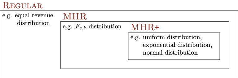
Finally, we’ll use the following notation for many of our theorem statements.
Definition 2.5 (Expected Order Statistics).
For a single-variate distribution with CDF , define:
- •
to be a random variable which is the highest of i.i.d. draws from .
- •
to be the expected value of the highest of i.i.d. draws from . That is, .
- •
to be the expected hazard rate of the highest of i.i.d. draws from . That is, . Note that the definition inside the expectation is intentional: we first find the highest sample, and then compute its hazard rate with respect to the original .
- •
to be the expected inverse hazard rate of the highest of i.i.d. draws from . That is, .
2.2 Virtual Value Preliminaries
A tool that we’ll repeatedly use throughout our results is the Myersonian theory of virtual values Myerson 1981.
Definition 2.6 (Virtual value).
For a single-dimensional distribution with CDF and PDF , define the virtual value with respect to as , with .
Note also that . The inverse of is well-defined when is non-decreasing, and unique when strictly increasing.
Theorem 2.1 (Myerson 1981).
The following conditions hold
- •
Let be regular. Then is monotone non-decreasing, and . Observe that is the set of all such that .
- •
If is not regular, it is still the case that satisfies .88 8 For readers not familiar with this particular claim, it follows by observing that is exactly the first-order condition for maximizing the revenue curve of .
- •
Finally, for all and , .99 9 This follows from the equivalence of expected virtual surplus and expected revenue. The expected revenue of the second-price auction with bidders is the LHS, and the expected virtual value of the winner is the RHS.
Observation 3.
Let be MHR. Then is unique.
Proof.
Observe that is strictly increasing in , and is weakly decreasing in . Therefore, cannot have multiple solutions. ∎
3 Best Responding in the Free Market Setting
In this section, we expand on the mathematics behind what it means to best-respond in the Free Market setting. Importantly, recall that every consumer must select a provider, even if their utility for each is negative. Our focus is on the symmetric case ( is symmetric, searching for a symmetric equilibrium). In Section 6 we consider extensions to the asymmetric case.
Consider the search for a symmetric equilibrium. The question we need to ask is “given that the other providers are setting price , is a best response for the remaining provider?” To resolve this, we first need to understand more precisely the payoff received by the remaining provider for setting price while the other set price .
Definition 3.1 (Star Operation).
Let be such that when all providers are setting price , and provider sets price , the probability that the consumer purchases from provider is . That is, the payoff to provider in this circumstance is .
Our choice of notation suggests that we will reason about best-responding as a single-item revenue problem, with the consumer’s value distribution defined by . Our goal will be to find sufficient conditions for there to exist a such that itself is the revenue-maximizing price for the distribution . Our plan is roughly as follows:
- •
Write an expression for .
- •
Observe that is necessary for to possibly be a symmetric equilibrium, by first-order conditions (Theorem 2.1). Show that this equation has a unique solution.
- •
If is regular or MHR, then first-order conditions suffice for to be a best response, and therefore is indeed a symmetric equilibrium (but this is not necessary for to be a symmetric equilibrium).
- •
Prove that if is with decreasing density, then is MHR.
Let’s quickly highlight some aspects of this plan. Typically, finding a closed form for potential equilibria, and establishing that sufficient conditions hold is a matter of solving systems of non-linear equations. Often, this process may be mathematically engaging, but not offer insight connecting the sufficient conditions to the conclusions. The final step of our outline (that implies MHR ) is still mostly “just math;” however, the rest of the outline leverages existing theory of Myersonian virtual values to make the rest of the math more intuitive.
Let’s now begin by writing an analytical expression for , , and . This will let us (a) compute the virtual value and (b) check whether is regular or MHR. Recall that is the probability that the consumer chooses to purchase from a provider priced at when the other are priced at . Below, observe that is the density of the maximum of draws from , after adding and subtracting .
Proposition 3.1.
Let . Let also .
- •
.
- •
.
- •
.
- •
.
Note that the definitions in Proposition 3.1 are referred to many times throughout the proofs of Propositions 3.2 and 3.3; the reader may want to keep them handy. The proof of Proposition 3.1 appears in Appendix A.
The following describes a condition that must be met as a result of first-order conditions in order to possibly have a symmetric equilibrium in the Free Market setting. Note that this holds for any , even those which are not MHR or regular.
Proposition 3.2.
Let . The only possible symmetric equilibrium in the Free Market setting is . If is regular, then is a symmetric equilibrium.
Proof.
By Theorem 2.1 and the definition of , in order for to be a best response to all other providers setting price , we must have . Note that this does not guarantee that is a best response; this is just a necessary first-order condition.
Observe that, using Proposition 3.1, many of the terms in (and ) simplify when , so we get:
Let’s first examine the numerator. The numerator integrates over all , the density , times the probability that exactly one of other draws from exceed (this is ). This is exactly the probability that one of draws is the second-highest, which is just . Another way to see that is just that , by definition, is the probability that a particular one of providers is the consumer’s favorite. But as is symmetric, and the price is the same for all providers, this is just . So now we wish to examine the denominator, with an extra factor of from the numerator:
All we have done above is multiply and divide by . But now the integral is interpretable: we are integrating over all , the number of ways to choose an ordered pair of draws (), times the density of at (this is ), times the probability that exceeds (), times the probability that the remaining items do not exceed (), times the hazard rate at . This is exactly computing the expected hazard rate of the second-highest of draws from ! Therefore, we immediately conclude that:
and therefore iff . Importantly, note that we have proven that for all , even those which are not equilibria, or otherwise related to , that . ∎
So at this point, we know know the unique candidate for a symmetric equilibrium (because it is the only candidate which satisfies first-order conditions of Theorem 2.1). If we can find sufficient conditions for to be regular (or MHR), then these first-order conditions suffice for to indeed be a symmetric equilibrium. We identify such sufficient conditions below (remember that Proposition 1.5 establishes that MHR alone does not suffice, so some stronger conditions are necessary):
Proposition 3.3.
Let be and have decreasing density. Then for all , is MHR.
Proof.
Lets first develop intuition for why is a convenient condition for reasoning about the starred distribution. Observe that each of the starred CDF/PDF/etc. functions are convolutions of the original CDF/PDF/etc. with . Unfortunately, just knowing that, for example, for all (which is guaranteed by MHR from Observation 2 (3)) is not enough for us to reason about these convolutions. But buys us something stronger, which is exactly what’s needed for the first half of the proof: not only is for all , but in fact everywhere, which does allow us to make direct substitutions into the convolution. To see this, consider attempting to manipulate using only Obs. 2 (4) for MHR—that for all —instead of what we use from the definition for . The second step of the proof is dealing with the additional terms outside of the integral. Surprisingly, also turns out to be the right condition to reason transparently about these additional terms, although more creativity is required here than in step one. We now proceed with the proof.
First, observe that if has decreasing density, then (so we may divide by ). Next, because is , recall by Observation 2 condition (7) that we have , and . Since , this implies that . Therefore, we get:
Similarly, we can write:
Therefore, we get:
The above inequality completes the “step one” referenced in the proof summary. Our remaining task is to show that:
as then we will have established that , and therefore is MHR. Observe that this is clearly true when , as the entire term above is —both (as can be seen by plugging it in to its definition or reasoning about the probability of ties at 0, which has probability 0) and . So the remaining case is when . Here, we derive the following, starting with the justification and then showing the equations.
The first inequality follows by definition of being from Observation 2 (7): . The second follows by dividing both sides by , which is strictly positive. The third line follows by evaluating the definition of from Proposition 3.1.
The fourth line then follows by multiplying both sides by , which is positive. The fifth line follows because when , and has decreasing density. The penultimate line follows as for all .
The final line follows from the following reasoning. Recall that denotes the probability that the consumer will choose to purchase a specific plan when that plan has price and all other plans have price . The probability that this occurs conditioned on having value for the specific plan is the probability that the consumer has utility for every other plan, or value , which occurs with probability exactly , and the previous term simply integrates this times over all .
Finally, observe that this inequality is exactly what we want, as:
because again, in this case. ∎
And now, we can wrap up the proof of Theorem 1.1, which claims that whenever is , the unique symmetric equilibrium in the Free Market setting for is for each provider to set price .
Proof of Theorem 1.1.
Note that Theorem 1.1 accomplishes several tasks:
- •
It establishes that a symmetric equilibrium exists subject to (which is not generally true without some assumptions, Proposition 1.5).
- •
It provides a clean closed form for this symmetric equilibrium.
- •
It establishes uniqueness of this equilibrium (even stronger: this is the only possible equilibrium for all ). This is important because it lets us reason about “the utility in the Free Market setting” without needing to worry about exactly which equilibrium we should be analyzing.
4 Comparing Consumer Utilities
In this section, we derive a Limit-Entry condition, which dictates when consumer utility is higher in the Limited Entry setting versus the Free Market. Note that our condition is well-defined even when no symmetric equilibrium exists in the Free Market setting. Let’s first recall the Limit-Entry condition from Section 1, which a distribution satisfies when
where again, is the expected inverse hazard rate of the highest of i.i.d. draws from and is the expected hazard rate of the second-highest of i.i.d. draws from . Recall that Theorem 1.2 states that consumer utility is higher in the Limited Entry setting versus the Free Market setting if and only if the Limit-Entry condition holds. The main result of this section is a proof of Theorems 1.2, and 1.3.
Proof of Theorem 1.2.
Let’s first compute the expected consumer utility in the Limited Entry setting.
Lemma 4.1.
The expected consumer utility at the unique equilibrium in the Limited Entry setting is .
Proof.
There are a total of providers, and recall from Observation 1 that the unique equilibrium has all prices set to . Therefore, the consumer’s expected payment is zero. The consumer picks their favorite plan, with value simply the maximum of i.i.d. draws from . Together, we see that the consumer’s expected utility at the unique symmetric equilibrium of the Limited Entry setting is . ∎
Now, let’s compute the expected consumer utility in the Free Market setting.
Lemma 4.2.
The expected consumer utility at the unique symmetric equilibrium (when it exists) in the Free Market setting is .
Proof.
There are a total of providers, and the unique symmetric equilibrium (when it exists) has all prices set to . Therefore, the consumers expected payment is (because the consumer must purchase a plan, even with negative utility for everything). The consumer’s value for their favorite plan is the maximum of i.i.d. draws from . Therefore, the consumer’s expected utility at the unique symmetric equilibrium of the Free Market setting is . ∎
We therefore see that the expected utility is higher in the Limited Entry setting versus Free Market if and only if . The remainder of the proof is rewriting this condition, using Myersonian virtual value theory in yet another way. We produce the steps below, and justify each step afterwards. Two of the three steps follow from basic algebra or a coupling argument. The middle step (line three) makes use of virtual value theory.
The first equivalence follows by a coupling argument. One way to draw the highest of draws from , or , is to take draws from , remove one uniformly at random, and then examine the highest remaining. With probability , the highest of the draws is excluded, so the highest remaining is . The rest of the time, a different draw is excluded and the highest of remains, giving . Hence in expectation, .
The second equivalence follows from Theorem 2.1, as . More familiarly, this is the fact that a second-price auction is revenue-maximizing, and that the revenue is equal to the virtual welfare of the highest-valued bidder in the iid setting. Recall that ; then .
The final equivalence follows by subtracting from both sides and multiplying by . ∎
Finally, we prove Theorem 1.3. Recall that Theorem 1.3 asserts that whenever is MHR with decreasing density, it satisfies the Limit-Entry condition. Recall that MHR alone is not enough to guarantee that there is an equilibrium in the Free Market setting for the Limited Entry setting to improve over, but that the condition is well-defined anyway. When is further , there is an equilibrium in both settings, and the consumer utility is always higher with Limited Entry (Corollary 1.4).
Proof of Theorem 1.3.
The proof will follow from the steps below (justification for each step is provided afterwards). If is MHR with decreasing density, then:
The first line follows because has decreasing density. Therefore for all , and certainly for any non-negative random variable (including ). The second line follows by simple algebra. The third line makes two steps. On the LHS, we observe that , so the left-hand sides are actually identical between the second and third lines. On the right-hand side, we just multiply the numerator and denominator by . The final implication again makes two steps. On the left-hand side, we observe that as is MHR, for all . Therefore, for any non-negative random variable (including ). On the right-hand side, we have used the equality , which will be proved shortly (and complete the proof).
The last line above completes the proof (once we establish the equality): we have shown that if is MHR with decreasing density, then the Limit-Entry Condition is satisfied. The remaining task is to prove Lemma 4.3, below.
Lemma 4.3.
.
Proof.
The first line is simply the definition of . The second line just rewrites . The third line observes that is the density of . Indeed, there are ways to choose a provider from , is the density of at , and is the probability that all other providers have . So we are integrating the density of at , times from to . This exactly computes the expected value of . The extra factor of is carried through. ∎
∎
5 Extension: Non-Zero Costs and Common Base-Value
In this section, we establish that our previous results hold verbatim when the provider faces a non-zero cost to provide for the consumer, or in the Common Base-Value model of Chawla et al. 2015. This section uses standard tricks from auction design to redefine the buyer’s value distribution as the seller’s profit distribution.Usually, these tricks adjust the distribution of study (e.g. by subtracting a constant). In our setting, due to the mandatory purchase, they actually have no impact on the distribution at all, and our results are independent of the (symmetric) per-consumer cost. We begin by defining non-zero cost.
Definition 5.1 (Non-zero cost).
Keep all aspects of the model the same, and additionally define a cost that each provider must pay per consumer covered. That is, if a provider covers a fraction of the market, and sets price , that provider’s payoff is .
To see why our model is independent of the cost , consider the following thought experiment. Instead of having the providers pay cost per consumer, tell every consumer that they must pay an additional , no matter which provider they choose. Importantly, because purchase is mandatory, this additional cost doesn’t affect the consumer’s decisions at all. So consumer decisions are exactly the same as in the zero-cost model. Moreover, because providers are paid an additional by the consumer to cover the cost, their payoff at a given price vector is exactly the same as if there were zero cost. We again emphasize that the key difference between our setting and typical single-item settings (where cost with value distribution is equivalent to zero cost with value distribution subtracting ) is the mandatory purchase. In single-item sale, the “don’t purchase” option becomes more attractive when the “purchase” option has cost increased by . But in our setting, there is no “don’t purchase” option, and all options uniformly increase in cost by .
Finally, it is easy to see that any strategy profile in the above-described thought experiment (where the consumer pays an additional , independent of choice) is identical to the strategy profile (i.e. increase all prices by ) if the providers pay cost per consumer covered. This is again because the consumer’s choice is invariant under increasing all prices by the same fixed amount. This allows us to conclude the following:
Proposition 5.1.
All previous results stated when the providers have zero cost hold verbatim when providers have non-zero cost. Specifically:
- •
If has a symmetric equilibrium in the Free Market setting with zero cost, then for all , has a symmetric equilibrium in the Free Market setting with cost (and the equilibrium adds to all prices).
- •
If admits a symmetric equilibrium in the Free Market setting with zero cost, then for any , the expected consumer utility at the unique symmetric equilibrium in the Limited Entry setting exceeds that at the unique symmetric equilibrium in the Free Market setting if and only if satisfies the Limit-Entry Condition.
It is easy to see that all other results for the zero-cost setting extend to any cost by the above two bullets. The same conclusions hold for an extension to Common Base-Value distributions as well. Note that the Common Base-Value setting may be relevant in our motivating example of health insurance, where a consumer has a base-value for being covered by any insurance at all.
Definition 5.2 (Common Base-Value Chawla et al. 2015).
A consumer’s valuation vector is drawn from a common base-value distribution if they first draw and then set .
Similarly to the above reasoning on costs, observe that a consumer with values or with values will purchase exactly the same plan at prices (again, because “not purchase” is not an option). Therefore, the common base-value can simply be treated as , because it does not impact any consumer choices, and all previous results immediately extend to this model as well.
Proposition 5.2.
All previous results stated when the consumers are drawn from a product distribution hold verbatim when consumers are instead drawn from a common base-value distribution. Specifically:
- •
If has a symmetric equilibrium in the Free Market setting, then for all base-value distributions , has a symmetric equilibrium in the Free Market setting. (It’s the same equilibrium.)
- •
If admits a symmetric equilibrium in the Free Market setting, then for all base-value distributions , the expected consumer utility at the unique symmetric equilibrium in the Limited Entry setting for exceeds that at the unique symmetric equilibrium in the Free Market setting for if and only if satisfies the Limit-Entry Condition.
6 Extension: Asymmetric Distributions
In this section, we extend our results on equilibria in the Free Market setting to asymmetric distributions. Here, we only prove existence results for certain kinds of equilibria rather than closed form solutions, hence it would not be possible to extend the Limit-Entry Condition without a significantly different approach. To be clear: we are in exactly the same model as the rest of the paper, but no longer assuming that is symmetric. We will still aim for sufficient conditions for a symmetric equilibrium to exist, but our extensions hold for restricted cases. Many of the lemmas in this section hold for general , and we will state them as such.
The structure of this section will closely parallel that of Section 3, and the proofs follow similar intuition with additional technical work. We begin by updating the definition of the star operation.
Definition 6.1 (Star Operation).
Let be such that when each provider sets price , and provider sets price , the probability that the consumer purchases from provider is . That is, the payoff to provider in this circumstance is .
Proposition 6.1.
Let . Let also . Then:
- •
.
- •
.
- •
.
- •
.
Like in Section 3, we establish that if is and decreasing density, then is MHR, for all .
Proposition 6.2.
Let be and decreasing density. Then for all , is MHR.
The proof parallels that of Proposition 3.3, and can also be found in Appendix B. Finally, we use this proposition to establish that an equilibrium exists for all two-provider instances with marginals.
Theorem 6.3.
Let be . Then there exists a pure equilibrium for .
Proof.
The proof will proceed by applying Brouwer’s fixed point theorem. There are two high-level steps. First, we must establish that the best-response function for player (responding to a price set by the other player) is well-defined and continuous (Lemma 6.4). Second, we must establish that it maps a compact domain to itself. The first step is fairly straight-forward, while the second step requires some creativity (and indeed the second step is messy to extend beyond two providers). We establish the first half of the proof for general . We begin first by establishing that the best response function is continuous for all when is MHR.
Lemma 6.4.
Let be MHR for all . Then the best response function which takes as input and outputs the best response price for provider is continuous.
Proof.
Because is MHR for all , we can actually write a closed form for the best response function . Indeed, because there is a unique satisfying the first order conditions of , this is the best response. We can therefore write:
recalling from Proposition 6.1 that:
where and . As is MHR, observe that is monotone strictly increasing, and also continuous (in fact, it is also differentiable). Therefore, the inverse is well-defined, and also continuous (in fact, differentiable).
Observe that our function is exactly the function which takes as input and outputs the such that . As we have noted that is continuous, is continuous as well, by the implicit function theorem. ∎
Now, we want to consider the function which takes as input a price vector and outputs . This function is continuous, since each coordinate is continuous. We just want to show that it maps a compact region to itself, and then Brouwer’s fixed point theorem will establish that an equilibrium exists.
So our plan is to find a value such that for all , , as well (from here, we will abuse notation and let denote the coordinate of our vector-valued function , which is also equal to the afore-defined ). We begin with the following observation.
Observation 4.
Let be MHR, and let . Then .
Proof.
Clearly, . Because is monotone increasing, it means that . ∎
Corollary 6.5.
Let . Then when .
Proof.
Crucially, observe that for all . Therefore, . This should be intuitive: if all prices increase by , then all of the probabilities of sale stay the same. This immediately implies that:
The last inequality follows as since is MHR for any . Let’s see now what the last line implies. It means certainly that , and therefore . We therefore conclude that is weakly increasing with respect to the non- coordinate, proving the corollary. ∎
Corollary 6.5 establishes is non-decreasing in the other provider’s price, and further, that when , then is maximized when for , and that . Then to conclude that we map a compact region to itself, we just need to show that .
Lemma 6.6.
For any , let be MHR for all . Let also . Then .
Proof.
Observe that in fact is independent of . To see this, recall that concerns only the probability that the consumer purchases provider when all prices are (and is its derivative with respect to ). Observe, however, that because the buyer must purchase an option even when their utility is negative for everything, that this probability is completely independent of . Therefore, this is actually equal to , which is just some finite number. Whenever , the condition is satisfied. ∎
Finally, we may now simply set to guarantee that it is at least as large as both. By the work above, maps to , and is continuous. Therefore it has a fixed point by Brouwer’s fixed point theorem, which is exactly a pure equilibrium. ∎
References
- Anton and Gertler [2004] James J Anton and Paul J Gertler. Regulation, local monopolies and spatial competition. Journal of Regulatory Economics, 25(2):115–141, 2004.
- Bulow and Klemperer [1994] Jeremy Bulow and Paul Klemperer. Auctions vs. negotiations. Technical report, National Bureau of Economic Research, 1994.
- Chawla et al. [2007] Shuchi Chawla, Jason D Hartline, and Robert Kleinberg. Algorithmic pricing via virtual valuations. In Proceedings of the 8th ACM conference on Electronic commerce, pages 243–251. ACM, 2007.
- Chawla et al. [2010] Shuchi Chawla, Jason D Hartline, David L Malec, and Balasubramanian Sivan. Multi-parameter mechanism design and sequential posted pricing. In Proceedings of the forty-second ACM symposium on Theory of computing, pages 311–320. ACM, 2010.
- Chawla et al. [2015] Shuchi Chawla, David Malec, and Balasubramanian Sivan. The power of randomness in bayesian optimal mechanism design. Games and Economic Behavior, 91:297–317, 2015.
- Chen and Li [2013] Yuxin Chen and Xinxin Li. Group buying commitment and sellers? competitive advantages. Journal of Economics & Management Strategy, 22(1):164–183, 2013.
- Dana Jr [2012] James D Dana Jr. Buyer groups as strategic commitments. Games and Economic Behavior, 74(2):470–485, 2012.
- Engel et al. [2002] Eduardo Engel, Ronald Fischer, and Alexander Galetovic. Competition in or for the field: which is better? Technical report, National Bureau of Economic Research, 2002.
- Hotelling [1929] Harold Hotelling. (1929): Stability in competition. Economic Journal, 39(4):57, 1929.
- Johnson et al. [2013] Eric J Johnson, Ran Hassin, Tom Baker, Allison T Bajger, and Galen Treuer. Can consumers make affordable care affordable? the value of choice architecture. PloS one, 8(12), 2013.
- McGuire and Riordan [1995] Thomas G McGuire and Michael H Riordan. Incomplete information and optimal market structure public purchases from private providers. Journal of Public Economics, 56(1):125–141, 1995.
- Myerson [1981] Roger B Myerson. Optimal auction design. Mathematics of operations research, 6(1):58–73, 1981.
- Pai and Vohra [2014] Mallesh M Pai and Rakesh Vohra. Optimal auctions with financially constrained buyers. Journal of Economic Theory, 150:383–425, 2014.
- Saban and Weintraub [2019] Daniela Saban and Gabriel Y Weintraub. Procurement mechanisms for assortments of differentiated products. Available at SSRN 3453144, 2019.
- Williams [2016] Jackson Williams. The patient protection and affordable care act meets the ‘persistently uninsured’. Social Policy & Administration, 50(4):452–466, 2016.
Appendix A Omitted Proofs from Section 3
Proposition 3.1.
Let . Let also .
- •
.
- •
.
- •
.
- •
.
Proof.
For the first bullet, denotes the probability that the consumer does not have highest utility for the lone provider () setting price . Observe that is the derivative of with respect to . If denotes the random variable that draws times from and takes the maximum, then adds , then is the CDF of , so is the PDF of . Observe also that the consumer will not purchase from the lone provider setting price iff .
One way to compute the probability that is to integrate over all possible values of (), the density of at times the probability that does not exceed . When , the probability that does not exceed is . When , the density of at is . So we may restrict the integral to the range . Finally, is exactly the probability that does not exceed , and is exactly the density of at , yielding the first bullet.
For the second bullet, observe that is integrating the density of some random variable from to . This random variable is supported on to . So if , the integral is , and we have that:
If , then the integral isn’t necessarily , but is instead , so an additional needs to be added. Observe that when , and is otherwise, as desired.
For the third bullet, we apply Leibniz’ integral rule, and take the derivative of with respect to . The derivative of with respect to is , and the derivative of with respect to is . So we get that:
Doing integration by parts, with and , and observing, crucially, that (so and ), we get:
Finally, observe that if , the terms at the right cancel. if , both terms are (and still cancel).
For the fourth bullet, we again apply Leibniz’ integral rule, and take the derivative with respect to . We get:
Again doing integration by parts, with and (so , ), we get:
Finally, observe that if , then the right two terms cancel. If , then we’re left with . Observe that when , , so the added term in the proposition statement is correct. ∎
Appendix B Omitted Proofs from Section 6
Proposition 6.1.
Let . Let also . Then:
- •
.
- •
.
- •
.
- •
.
Proof.
For the first bullet, denotes the probability that the consumer does not have highest utility for the provider setting price . Observe that is the derivative of with respect to . If denotes the random variable that draws from each of (), then adds and takes the maximum, then is the CDF of , so is the PDF of . Observe also that the consumer will not purchase from provider iff .
One way to compute the probability that is to integrate over all possible values of (), the density of at times the probability that does not exceed . When , the probability that does not exceed is . When , the density of at is . So we may restrict the integral to the range . Finally, is exactly the probability that does not exceed , and is exactly the density of at , yielding the first bullet.
For the second bullet, observe that is integrating the density of some random variable from to . This random variable is supported on to . So if , the integral is , and we have that:
If , then the integral isn’t necessarily , but is instead , so an additional term needs to be added. Observe that when , this is exactly the term added in the statement. When , the added term is (and should be , by above).
For the third bullet, we apply Leibniz’ integral rule, and take the derivative of with respect to . The derivative of with respect to is , and the derivative of with respect to is . So we get that:
Doing integration by parts, with and , and observing, crucially, that (so and ), we get:
Finally, observe that if , the terms at the right cancel. if , both terms are (and still cancel).
For the fourth bullet, we again apply Leibniz’ integral rule, and take the derivative with respect to . We get:
Again doing integration by parts, with and (so , ), we get:
Finally, observe that if , then the right two terms cancel. If , then we’re left with . Observe that when , , so the added term in the proposition statement is correct. ∎
We continue with another missing proof that parallels Section 6.
Proposition 6.2.
Let be and decreasing density. Then for all , is MHR.
Proof.
First, observe that if has decreasing density, then (so we may divide by ). Next, recall by Observation 2 that we have , and . Therefore, we get:
Similarly, we can write:
Therefore, we get:
So if we can show that
then we will have established that , and therefore is MHR. Observe that this is clearly true when , as the entire term above is (because and for all ). So the remaining case is when . Here, we derive the following (justification for each equation follows).
The first inequality follows by definition of being . The second follows by dividing both sides by , which is positive. The third line follows by evaluating the definition of .
The fourth line then follows by multiplying both sides by , which is positive. The fifth line follows as for all , . The penultimate line follows because for all , has decreasing density (and therefore for all ).
The final line follows from the following reasoning. Recall that denotes the probability that the buyer will choose to purchase item when item has price and all other items have price . The probability that this occurs conditioned on is exactly , and the previous term simply integrates this times over all .
Finally, observe that this inequality is exactly what we want, as (the first line below is exactly what we just proved above, and the final line is our remaining task).
∎
Appendix C Calculations for Examples
Recall that denotes the probability that a consumer drawn from does not have the highest utility for the lone provider setting price , when the other providers are setting price p. Then, the expected payoff of the lone provider (n) in this circumstance is .
Consider the following class of examples, which we’ll refer to as . Note that the hazard rate is the most interesting part of the distribution, and the CDF ensures such a distribution is well-defined.
x.p. for
x.p.
for
Observation 5.
For all , is MHR.
Lemma C.1.
There exists , such that is anti-MHR.
Proof.
We start by defining an even more general class of MHR distributions. In particular, let be any two positive constants, and let be any distribution that satisfies the following properties:
and for
and and for
Clearly, is MHR because , . We now compute to see whether is MHR or not.
Note this last term can be reformulated as:
and is thus lower bounded by a constant. We can now rewrite the product as follows:
(assume worst case )
(with , because )
Note that can be made as large as possible for fixed , and so we get the following:
Thus, for any MHR distribution defined as above, * is anti-MHR.
We now provide an example distribution () that satisfies the conditions of the distribution class characterized by . Indeed, the distribution is just a special case of the distribution . By setting , , and for the distribution , we obtain the distribution .
Thus, MHR can, in fact, lead to non-MHR (and even lead to anti-MHR) . In other words, non-decreasing can lead to non-monotone (and even lead to non-increasing) because the MHR condition is violated, as shown in the example above where and .
Therefore, there exists , such that is MHR but is anti-MHR.
∎
We now define a setting where the consumer is drawn from where is the distribution we defined above.
Assume providers set price , and provider sets price . The consumer has external options valued at and will only purchase from the lone provider () at price if the utility from provider is better than the utility from providers .
Provider has payoff with and and sets the revenue maximizing price arg
arg
arg
arg
We now restrict our attention to the case where there are only two providers (). Consumer valuations are drawn from . Thus, provider n (i.e. ) sets the revenue maximizing price arg = arg
Consider the case where . Whenever , provider will never be chosen since , so we get the following integral bounds:
arg
= arg )
We can now conclude that, in the two-provider scenario, for all , when provider uses the price , provider best responds by setting the revenue maximizing price arg )
We now use specific instances of this best-response result to prove the lemmas below.
Lemma C.2.
When , , , the MHR distribution has no symmetric equilibrium.
Proof.
When there are only two providers (), our setting then becomes that of a consumer drawn from . In particular for , i.e. when the consumer is drawn from , provider is best responding by setting the revenue maximizing price arg ) = arg )
Using the formula from Proposition , we compute the hazard rate of the second highest value
which gives the unique potential symmetric equilibrium price
Provider is now best responding to this potential symmetric equilibrium price by setting the revenue maximizing price defined above as arg ). Solving for this gives , at a revenue of .
The prices are not equal, thus we don’t have symmetric equilibrium
Therefore, when , , , the MHR distribution has no symmetric equilibrium.
∎
Observation 6.
If is MHR, then is weakly decreasing in . If is anti-MHR, then is weakly increasing in .
Lemma C.3.
When , , and , satisfies the Limit Entry Condition, but does not have a symmetric equilibrium in the Free Market setting.
Proof.
We refer to the same example above (in Lemma ) where we had , , and . We showed that it has no symmetrical equilibrium. However, any guarantees that and thus satisfies the Limit-Entry Condition. In particular, when , satisfies the Limit Entry Condition but does not have a symmetric equilibrium in the Free Market setting.
Therefore, when , , and , satisfies the Limit Entry Condition, but does not have a symmetric equilibrium in the Free Market setting.
∎
Lemma C.4.
When , , and , has a symmetric equilibrium in the Free Market setting, but does not satisfy the Limit Entry Condition.
Proof.
We again consider the two-provider setting () where
the consumer is drawn from . In this instance, we set , and , i.e. when the consumer is drawn from .
Using the formula from Proposition , we compute the hazard rate of the second highest value
which gives the unique potential symmetric equilibrium price
Provider is now best responding to this potential symmetric equilibrium price by setting the revenue maximizing price defined above as arg ) for . Solving for this gives and revenue = .
We thus have a symmetrical equilibrium since the best response to is .
We now check if the Limit Entry condition is satisfied. First, we compute the terms for the Limit-Entry Condition as follows:
(exact)
which gives
Note that which violates the Limit-Entry Condition.
Therefore, when , , and , has a symmetric equilibrium in the Free Market setting, but does not satisfy the Limit Entry Condition.
∎