Social-WaGDAT: Interaction-aware Trajectory Prediction via Wasserstein Graph Double-Attention Network
Abstract
Effective understanding of the environment and accurate trajectory prediction of surrounding dynamic obstacles are indispensable for intelligent mobile systems (like autonomous vehicles and social robots) to achieve safe and high-quality planning when they navigate in highly interactive and crowded scenarios. Due to the existence of frequent interactions and uncertainty in the scene evolution, it is desired for the prediction system to enable relational reasoning on different entities and provide a distribution of future trajectories for each agent. In this paper, we propose a generic generative neural system (called Social-WaGDAT) for multi-agent trajectory prediction, which makes a step forward to explicit interaction modeling by incorporating relational inductive biases with a dynamic graph representation and leverages both trajectory and scene context information. We also employ an efficient kinematic constraint layer applied to vehicle trajectory prediction which not only ensures physical feasibility but also enhances model performance. The proposed system is evaluated on three public benchmark datasets for trajectory prediction, where the agents cover pedestrians, cyclists and on-road vehicles. The experimental results demonstrate that our model achieves better performance than various baseline approaches in terms of prediction accuracy.
1 Introduction
In order to navigate safely in dense traffic scenarios or crowded areas full of vehicles and pedestrians, it is crucial for autonomous vehicles or mobile robots to forecast future behaviors of surrounding interactive agents accurately and efficiently lefevre2014survey. For short-term prediction, it may be acceptable to use pure physics based methods. However, due to the uncertain nature of future situations, the system for long-term prediction is desired to not only allow for interaction modeling between different agents, but also to figure out traversable regions delimited by road layouts as well as right of way compliant to traffic rules. Figure 1 illustrates several traffic scenarios where interaction happens frequently and the drivable areas are heavily defined by road geometries. For instance, at the entrance of roundabouts or unsignalized intersections, the future behavior of an entering vehicle highly depends on whether the conflicting vehicles would yield and leave enough space for it to merge. In addition, for vehicle trajectory prediction, kinematic constraints should be satisfied to make the trajectories feasible and smooth.
There have been extensive studies on the prediction of a single target entity, which consider the influences of its surrounding entities hong2019rules; chai2019multipath; alahi2016social; gupta2018social. However, such approaches only care about a one-way interaction, but ignore the potential interactions in the opposite way. Recent works have tried to address this issue by simultaneous forecasting for multiple agents deo2018convolutional; deo2018would; zhao2019multi. However, most of these methods just use concatenation or pooling operations to blend the features of different agents without explicit relational reasoning. Moreover, they are not able to model higher-order interactions beyond adjacent entities. In this work, we make a step forward to model the interactions explicitly with a spatio-temporal graph representation and the message passing rules defined by graph networks battaglia2018relational, which enables permutation invariance and mutual effects between pairs of entities. Moreover, since it is also essential to figure out which of the other agents have the most significant influence on a certain agent, we employ a double-attention mechanism on both topological and temporal features.
Besides models that directly maximize the data likelihood, deep generative models such as generative adversarial networks (GAN), variational auto-encoder (VAE) and their conditional variants have been widely applied to representation learning and distribution approximation tasks goodfellow2014generative; kingma2013auto. Despite that VAE is a highly flexible latent variable model with encoder-decoder architecture which makes the posterior of the latent variable as similar as its prior (usually a normal distribution), the two distributions do not match well in many tasks, which breaks the consistency of the model. Also, although GAN have achieved satisfying performance on image generation tasks, it usually suffers from mode collapse problems especially when applied to sequential data under the conditional setting. Some variants of VAE ma2019; zhao2017infovae have been developed to mitigate these drawbacks by incorporating information theory, which are similar to the generative component in this work.
The main contributions of this paper are summarized as:
We propose a generic trajectory forecasting system with relational reasoning between interactive agents to predict pedestrian and vehicle trajectories.
We design a graph double-attention network (GDAT) to extract and update node features for spatio-temporal dynamic graphs with a novel topological attention mechanism based on a kernel function. The main advantages of GDAT are three-fold: (a) It can be applied to flexible number of agents with the property of permutation invariance, which enhances generalization ability; (b) It can model high-order interactions by multiple loops of message passing; (c) The attention mechanism provides a heuristic for multi-agent interaction modeling.
We incorporate an efficient kinematic constraint layer to ensure physical feasibility for vehicle trajectory prediction, which can also smooth the trajectories and reduce prediction error.
We validate the proposed system on multiple trajectory forecasting benchmarks and the system achieves the state-of-the-art performance.
The remainder of the paper is organized as follows. Section 2 provides a brief overview on state-of-the-art related research. Section 3 presents a generic problem formulation for trajectory prediction tasks. Section 4 illustrates the proposed forecasting system Social-WaGDAT. In Section 5, the proposed system is applied to interactive pedestrian and vehicle trajectory prediction based on real-world benchmark datasets. The performance is compared with baseline methods in terms of widely-used evaluation metrics. Finally, Section 6 concludes the paper.

2 Related Work
In this section, we provide a brief literature review on related research and illustrate the distinction and advantages of the proposed generative trajectory prediction framework.
Trajectory and Behavior Prediction
Extensive research has been conducted on trajectory prediction for pedestrians and on-road vehicles. Early literature mainly introduced physics-based or rule-based approaches such as state estimation techniques applied to kinematic models (e.g. constant velocity model), which can only perform well for short-term prediction with very limited model capacity liu2016vehicle; scharcanski2010particle. As machine learning techniques are studied more extensively, people began to employ learning-based models such as hidden Markov models wang2018learning, Gaussian mixture models li2018generic; Jiachen_ITSC18-2, dynamic Bayesian network kasper2012object and inverse reinforcement learning sun2018probabilistic. In recent years, many deep learning models have been proposed, which enables more flexibility and capacity to capture underlying interactive behavior patterns fernando2018soft+; lee2017desire; rudenko2019human; xu2018encoding; liang2019peeking; ma2019trafficpredict; Jiachen_IROS19; li2018development; huang2019uncertainty; su2019potential. However, physics-based feasibility constraints are usually ignored in learning-based methods. In this paper, we address interaction modeling and introduce a probabilistic trajectory prediction system based on deep generative models with interpretation from information theory, which also takes feasibility constraints into consideration.
Relational Reasoning and Graph Networks
The goal of relational reasoning is to figure out the relationships among different entities, such as image pixels wang2018non, words or sentences lin2017structured, human skeletons battaglia2016interaction or interactive moving agents zambaldi2018relational; choi2019looking. A typical representation of the whole context is to formulate a graph, where object states are node features and their relationships are edge features. Recently, graph networks (GN) are employed widely as a tool of graph-based learning, where there is no restriction on the message passing rules. Most existing works focused on the approximation function parameterized by deep neural network due to its high flexibility, which leads to graph neural networks (GNN). In this paper, we design a graph network with both topological and temporal attention mechanisms to capture underlying patterns of situation evolution.
Deep Generative Modeling
One of the advantages of generative modeling lies in the data distribution learning without supervision. Coupled with highly flexible deep networks, deep generative models have achieved satisfying performance in image generation, style transfer, sequence synthesis tasks, etc. Besides GAN and VAE, the Wasserstein auto-encoder (WAE) tolstikhin2017wasserstein was proposed from the optimal transport point of view, which encourages the consistency between the encoded latent distribution and the prior. Also, zhao2017infovae proposed a variant of VAE combined with information theory and a similar approach was proposed in ma2019.
3 Problem Formulation
The goal of this work is to predict future trajectories for multiple interactive agents based on their historical states and context information, where the number of involved agents may vary in different cases. Without loss of generality, we assume there are agents in the scene. We denote a set of trajectories covering the historical and forecasting horizons ( and ) as , where is the 2D coordinate in the world space or pixel space and is the heading angle, which is not necessary for pedestrian prediction. We also denote a sequence of context information (images or tensors) as for global context or for the local context of each agent. The future information is accessible during training. The trajectory and context information can be transformed to arbitrary format within the model as long as the output is consistent. Then we aim to approximate the conditional distribution with the proposed method. Note that we only deal with fixed scenes in this work.
4 Social-WaGDAT
In this section, we first provide an overview of the key modules and the architecture of the proposed generative trajectory prediction system. The detailed theories and model design of each module will then be further illustrated.
4.1 System Overview
The detailed architecture of Social-WaGDAT is shown in Figure 2, where a standard encoder-decoder architecture is employed. There are three key components: a deep feature extractor, an encoder with graph generation and processing module and a decoder with kinematic constraint layer. First, the feature extractor outputs state, relation and context feature embeddings from both history and future information, which includes the trajectories of the involved interactive agents and a sequence of context density maps and mean velocity fields. The extracted features are utilized to generate a spatio-temporal graph for both the history and the future respectively, in which the node attributes are updated with a double-attention mechanism. Then the new node attributes are transformed from the feature space into a latent space by an encoding function. Finally, the decoder generates feasible and realistic future trajectories for all the involved agents. The number of agents can be flexible in different cases due to the weight sharing and permutation invariance of graph representation. All the components are implemented with deep neural networks thus can be trained end-to-end efficiently and consistently.
4.2 Feature Extraction
The feature extractor consists of three parts: State MLP, Relation MLP and Context CNN. The State MLP embeds the position, velocity and heading information into a state feature vector for each agent. The Relation MLP embeds the relative information between each pair of agents into a relation feature vector, where the order of the two involved agents does matter since different orders correspond to different edges in the downstream graph representation. The relative information can be either the distance and relative angle (in a 2D polar coordinate) or the differences between the positions of the two agents along two axes (in a 2D Cartesian coordinate). The Context CNN extracts spatial features for each agent from a local occupancy density map () as well as heuristic features from a local velocity field () centered on the corresponding agent. The reason of using occupancy density maps instead of real scene images is to remove redundant information and efficiently represent data-driven drivable regions. The above procedures are applied at each time step, which generate a sequence of state, relation and context feature embeddings, respectively.
4.3 Encoder with GDAT
After obtaining the extracted features, a history graph (HG) and a future graph (FG) are generated respectively to represent the information related to the involved agents, where the state features and context features are concatenated to be the node attributes and the relation features are used as edge attributes. Note that the edge attributes are different for the same edge with different directions, which encode spatial relationship. The HG and FG are generated and processed in a similar fashion but with different time stamps. The number of nodes (agents) in a graph is assumed to be fixed, but the edges are eliminated if the spatial distance between two nodes is larger than a threshold. Therefore, the graph topology at different time steps may vary but not influence the following procedures.
The proposed graph double-attention network consists of two consecutive layers: a topological attention layer which updates node attributes from the spatial or topological perspective, and a temporal attention layer which outputs a high-level feature embedding for each node, which summaries both the topological and temporal information. Assume there are totally nodes (agents) in a graph, We denote a graph as , where and . and are the dimensions of node attributes and edge attributes.
Topological Attention Layer
The inputs of this layer are the original generated graphs and the output is a new set of node attributes which can capture local structural properties. The topological attention coefficients (showing the significance of node w.r.t. node ) are calculated by
| (1) |
where is the neighbor nodes with direct edges to node , is a prior attention coefficient which provides inductive bias from prior knowledge, and are weight parameters to adjust the relative significance of node attributes and edge attributes when computing attention coefficients. The intuition is that the agents with similar node attributes to the objective agent or with small spatial distance should be paid more attention to. In this work, we set implying no prior attention bias while more exploration on incorporating prior knowledge is left for future work. Then the node attributes are updated by
| (2) |
The procedures of node attribute update are applied to each time step and the weight matrices and vectors are shared across different time steps. We also employ the multi-head attention mechanism velivckovic2017graph to boost model performance by adjusting and , where the node attributes obtained by different attention coefficients are concatenated into a whole vector. The above message passing procedures can be applied multiple times to capture high-order interactions.
Temporal Attention Layer
The input of this layer is the output of the topological attention layer, which is a set of node attributes . The output is a set of highly abstract node attributes which will be further processed by the downstream modules. The temporal attention coefficients is
| (3) | ||||
where is a weight vector parameterizing the attention function. Then the node attributes are updated by
| (4) |
The multi-head attention mechanism can also be employed by using multiple different with average or concatenation.
Feature Encoding
The historical and future node attributes are concatenated and transformed by an encoding function to obtain the latent variable , which is given by
| (5) |
4.4 Decoder with Kinematic Constraint

We employ a similar method in ma2019 to impose a kinematic constraint cell to enforce feasible trajectory prediction following the recurrent unit, which is shown in Figure. 3. The bicycle model is a widely used nonlinear model to approximate the kinematics of vehicles, which has a continuous form
| (6) |
where are the coordinates of the center of mass, is the inertial heading and is the speed of the vehicle. is the angle of the current velocity of the center of mass with respect to the longitudinal axis of the car. We denote , and . Then the discretized version of the equations (6) can be written as
| (7) |
Here we provide an instance for the agent . The inputs of the gated recurrent unit (GRU) are the node attribute at the first step and zero paddings for the following steps. The outputs are the raw at each step which are truncated by a saturation function in order to restrict the accelerations in the feasible ranges. Then the kinematic cell takes in a sequence of and outputs future trajectories. If is not a prior knowledge or cannot be observed, then we can either approximate it with a constant or make it an independent output.
4.5 Loss Function and Training
In this part, we put forward a variant of generative modeling method, which is formulated similar in ma2019 and zhao2017infovae. In order to keep consistent with other literature on generative models, we use the same notations: denotes the predicted trajectories, denotes the latent variable and denotes the condition variable which is historical features. These notations were used for other purposes in previous sections.
The optimization problem can be written as
| (8) | ||||
Since the whole system is fully differentiable, we can train the network end-to-end by the Adam optimizer kingma2014adam and the loss function is given by
| (9) | ||||
where is a weight parameter to adjust the relative importance of the reconstruction loss and is the total number of training agents, is Kullback-Leibler divergence and MMD is maximum mean discrepancy. If , then the loss function degenerates to the pure -norm loss.
| Scenes | LR | P-LSTM | S-LSTM | S-GAN | S-GAN-P | S-Ways | SoPhie | Social-WaGDAT |
|---|---|---|---|---|---|---|---|---|
| ETH | 1.33 / 2.94 | 1.13 / 2.38 | 1.09 / 2.35 | 0.81 / 1.52 | 0.87 / 1.62 | 0.39 / 0.64 | 0.70 / 1.43 | 0.52 / 0.91 |
| HOTEL | 0.39 / 0.72 | 0.91 / 1.89 | 0.79 / 1.76 | 0.72 / 0.61 | 0.67 / 1.37 | 0.39 / 0.66 | 0.76 / 1.67 | 0.61 / 0.87 |
| UNIV | 0.82 / 1.59 | 0.63 / 1.36 | 0.67 / 1.40 | 0.60 / 1.26 | 0.76 / 1.52 | 0.55 / 1.31 | 0.54 / 1.24 | 0.43 / 1.12 |
| ZARA1 | 0.62 / 1.21 | 0.44 / 0.84 | 0.47 / 1.00 | 0.34 / 0.69 | 0.35 / 0.68 | 0.44 / 0.64 | 0.30 / 0.63 | 0.33 / 0.62 |
| ZARA2 | 0.77 / 1.48 | 0.51 / 1.16 | 0.56 / 1.17 | 0.42 / 0.84 | 0.42 / 0.84 | 0.51 / 0.92 | 0.38 / 0.78 | 0.32 / 0.70 |
| AVG | 0.79 / 1.59 | 0.72 / 1.53 | 0.72 / 1.54 | 0.58 / 1.18 | 0.61 / 1.21 | 0.46 / 0.84 | 0.54 / 1.15 | 0.44 / 0.84 |
| P-LSTM | S-Forces | S-LSTM | S-GAN | CAR-Net | S-ATT | DESIRE | Social-WaGDAT | |
| 38.12 / 58.63 | 36.48 / 58.14 | 33.19 / 56.38 | 28.67 / 44.35 | 25.72 / 51.80 | 33.28 / 55.86 | 35.38 / 57.62 | 22.52 / 38.27 |
| Baseline Methods | Social-WaGDAT | |||||||||
|---|---|---|---|---|---|---|---|---|---|---|
| Scenes | Time | CVM | P-LSTM | S-LSTM | S-GAN | S-ATT | ||||
| RA | 1.0s | 0.79 / 1.04 | 0.70 / 0.94 | 0.44 / 0.62 | 0.34 / 0.48 | 0.32 / 0.49 | 0.27 / 0.41 | 0.31 / 0.45 | 0.24 / 0.36 | 0.24 / 0.35 |
| 2.0s | 1.54 / 2.73 | 1.24 / 2.04 | 0.93 / 1.66 | 0.69 / 1.24 | 0.84 / 1.72 | 0.67 / 1.22 | 0.76 / 1.26 | 0.63 / 1.15 | 0.60 / 1.01 | |
| 3.0s | 2.27 / 3.91 | 1.75 / 2.98 | 1.44 / 2.71 | 1.10 / 2.15 | 1.51 / 3.15 | 1.01 / 2.11 | 1.19 / 2.34 | 0.94 / 2.04 | 0.86 / 1.83 | |
| 4.0s | 2.73 / 4.02 | 2.09 / 4.21 | 1.86 / 4.27 | 1.56 / 3.25 | 1.93 / 3.50 | 1.34 / 2.84 | 1.51 / 2.89 | 1.26 / 2.55 | 1.08 / 2.21 | |
| 5.0s | 2.90 / 4.38 | 2.35 / 5,39 | 2.17 / 5.12 | 2.11 / 4.70 | 2.13 / 4.86 | 1.85 / 4.41 | 2.13 / 4.24 | 1.65 / 3.98 | 1.31 / 3.34 | |
| UI | 1.0s | 0.88 / 1.14 | 0.74 / 1.00 | 0.50 / 0.70 | 0.41 / 0.57 | 0.38 / 0.57 | 0.40 / 0.59 | 0.41 / 0.61 | 0.37 / 0.55 | 0.36 / 0.54 |
| 2.0s | 1.64 / 2.85 | 1.30 / 2.14 | 1.00 / 1.79 | 0.82 / 1.49 | 0.99 / 2.04 | 0.81 / 1.41 | 0.87 / 1.56 | 0.78 / 1.38 | 0.74 / 1.31 | |
| 3.0s | 2.44 / 4.33 | 1.88 / 3.34 | 1.63 / 3.26 | 1.34 / 2.70 | 1.79 / 3.71 | 1.21 / 2.46 | 1.25 / 2.32 | 1.15 / 2.12 | 1.07 / 2.04 | |
| 4.0s | 2.91 / 4.27 | 2.39 / 4.05 | 2.22 / 4.19 | 1.95 / 4.16 | 2.43 / 4.50 | 1.86 / 3.98 | 1.93 / 4.26 | 1.78 / 3.80 | 1.63 / 3.56 | |
| 5.0s | 3.14 / 5.02 | 2.77 / 4.33 | 2.69 / 4.64 | 2.65 / 4.87 | 2.85 / 4.90 | 2.52 / 4.57 | 2.44 / 4.51 | 2.27 / 3.90 | 1.99 / 3.85 | |
| HR | 1.0s | 0.33 / 0.50 | 0.39 / 0.54 | 0.36 / 0.52 | 0.40 / 0.53 | 0.38 / 0.53 | 0.42 / 0.51 | 0.44 / 0.56 | 0.40 / 0.54 | 0.40 / 0.53 |
| 2.0s | 0.81 / 1.30 | 0.80 / 1.41 | 0.80 / 1.49 | 0.69 / 1.13 | 0.72 / 1.43 | 0.71 / 1.26 | 0.73 / 1.49 | 0.68 / 1.31 | 0.67 / 1.28 | |
| 3.0s | 1.15 / 2.00 | 1.23 / 2.28 | 1.29 / 2.49 | 1.00 / 1.81 | 1.19 / 2.31 | 0.91 / 1.75 | 0.98 / 1.97 | 0.88 / 1.78 | 0.87 / 1.78 | |
| 4.0s | 1.45 / 2.45 | 1.64 / 3.04 | 1.79 / 3.49 | 1.34 / 2.51 | 1.59 / 2.94 | 1.33 / 2.44 | 1.58 / 2.78 | 1.34 / 2.40 | 1.31 / 2.31 | |
| 5.0s | 1.71 / 3.25 | 1.95 / 3.26 | 2.19 / 3.87 | 1.68 / 3.22 | 1.89 / 3.04 | 1.66 / 3.13 | 1.81 / 3.34 | 1.62 / 2.97 | 1.57 / 2.88 | |
5 Experiments
In this section, we validate the proposed method on three publicly available benchmark datasets for trajectory prediction of pedestrians and on-road vehicles. The results are analyzed and compared with state-of-the-art baselines.
5.1 Datasets
Here we briefly introduce the datasets below. Please refer to the supplementary materials for details about the data processing procedures.
ETH ETH and UCY UCY: These two datasets are usually used together in literature, which include top-down-view videos and image annotations of pedestrians in both indoor and outdoor scenarios. The trajectories were extracted in the world space.
Stanford Drone Dataset (SDD)SDD: The dataset also contains a set of top-down-view images and the corresponding trajectories of involved entities, which was collected in multiple scenarios in a university campus full of interactive pedestrians, cyclists and vehicles. The trajectories were extracted in the image pixel space.
INTERACTION Dataset (ID)interactiondataset: The dataset contains naturalistic motions of various traffic participants in a variety of highly interactive driving scenarios. Trajectory data was collected using drones and traffic cameras.
The semantic maps of scenarios and agents’ trajectories are provided. We consider three types of scenarios: roundabout (RA), unsignalized intersection (UI) and highway ramp (HR). The trajectories were extracted in the world space.
5.2 Evaluation Metrics and Baselines
We evaluate the model performance in terms of average displacement error (ADE) defined as the average distance between the predicted trajectories and the ground truth over all the involved entities within the prediction horizon, as well as final displacement error (FDE) defined as the deviated distance at the last predicted time step.
For the ETH, UCY and SDD dataset, we predicted the future 12 time steps (4.8s) based on the historical 8 time steps (3.2s). For the ID dataset, we predicted the future 10 time steps (5.0s) based on the historical 4 time steps (2.0s).
We compared the performance of our proposed method with the following baseline approaches: Constant Velocity Model (CVM), Linear Regression (LR), Probabilistic LSTM (P-LSTM) Jiachen_ICRA19, Social Forces (S-Forces) luber2010people, Social LSTM (S-LSTM) alahi2016social, Social GAN (S-GAN and S-GAN-P) gupta2018social, Social Attention (S-ATT) vemula2018social, Social Ways (S-Ways) amirian2019social, SoPhie sadeghian2019sophie, CAR-Net sadeghian2018car and DESIRE lee2017desire. Please refer to the reference papers for more details.
5.3 Implementation Details
A batch size of 64 was used and the models were trained for 100 epochs using Adam with an initial learning rate of 0.001. The models were trained on a single TITAN X GPU. We used a split of 70%, 10%, 20% as training, validation and testing data. Please refer to supplementary materials for more details on the model architecture.
5.4 Quantitative Analysis
ETH and UCY Datasets: The comparison of the proposed Social-WaGDAT and baseline methods in terms of ADE and FDE is shown in Table 1. Some of the reported statistics are adopted from the original papers. It is not surprising that the linear model performs the worst in general since it does not consider any social interactions or context information. An exception is the HOTEL scenario since most trajectories are relatively straight and can be well approximated by line segments. The P-LSTM is able to achieve smaller prediction error than LR due to the larger model capacity and flexibility of recurrent neural network, although it also predicts solely based on the individual’s historical trajectories. The S-LSTM considers the interactions between entities by using a social pooling mechanism. The S-GAN and S-Ways further improve the performance by introducing deep generative modeling. Both SoPhie and our method leverage the trajectory and context information, but in different ways. Our model can achieve better performance owing to the explicit interaction modeling with graph neural networks and more compact distribution learning with conditional Wasserstein generative modeling. In general, our approach achieves the smallest average ADE and FDE across different scenes.
Stanford Drone Dataset: The comparison of results is provided in Table 2, where the ADE and FDE are reported in the pixel distance. Note that we also included cyclists and vehicles in the test set besides pedestrians. Similarly, the P-LSTM performs the worst due to lack of relational reasoning. The S-Forces incorporates interaction modeling from an energy-based perspective, while the S-ATT and CAR-Net utilize attention mechanisms, which leads to better accuracy. The S-GAN and DESIRE both solve the task from a probabilistic perspective by learning implicit data distribution and latent space representations, respectively. Our approach achieves the best performance in terms of prediction error, which implies the superiority of explicit interaction modeling and necessity of leveraging both trajectory and context information. The prediction error is reduced by 12.1% with respect to the best baseline method.
INTERACTION Dataset: We finally compare the model performance on the real-world driving dataset in Table 3. Here we only involved the baseline approaches whose codes are publicly available. Although we trained a unified prediction model on different scenarios simultaneously, we analyzed the results for each type of scenario separately. To allow for fair comparison, here we only compare our model with baseline methods since they do not leverage context information. In the HR scenarios, the linear model CVM has a good performance in general since most vehicles go straight along the lane without obvious velocity changes within a short period, which makes the assumption of constant velocity well applicable. But the learning-based models may be negatively affected by some subtle patterns learned from data and redundant information in such scenarios, especially for short-term prediction (e.g. 1.0s). As the prediction horizon increases, the results of baseline methods are comparable while our model achieves the best performance. The future behaviors in HR scenarios are relatively easy to forecast so our method did not achieve a significant improvement. In the RA and UI scenarios, however, the superiority of the proposed system is more distinguishable. It is shown that CVM performs the worst across all forecasting horizons since turning behaviors, negotiation and interaction between vehicles happen frequently, which makes the assumption of constant velocity much less applicable. The P-LSTM has a slightly better performance by using the recurrent network. While the S-LSTM, S-GAN and S-ATT incorporate interaction modeling by different strategies which further reduce the prediction error, our model still performs the best. This implies the advantages of the graph representation for interaction modeling. By using our full model , the prediction error is reduced by 29.4%, 21.1% and 8.8% in RA, UI and HR with respect to the best baseline method, respectively.
5.5 Qualitative and Ablative Analysis
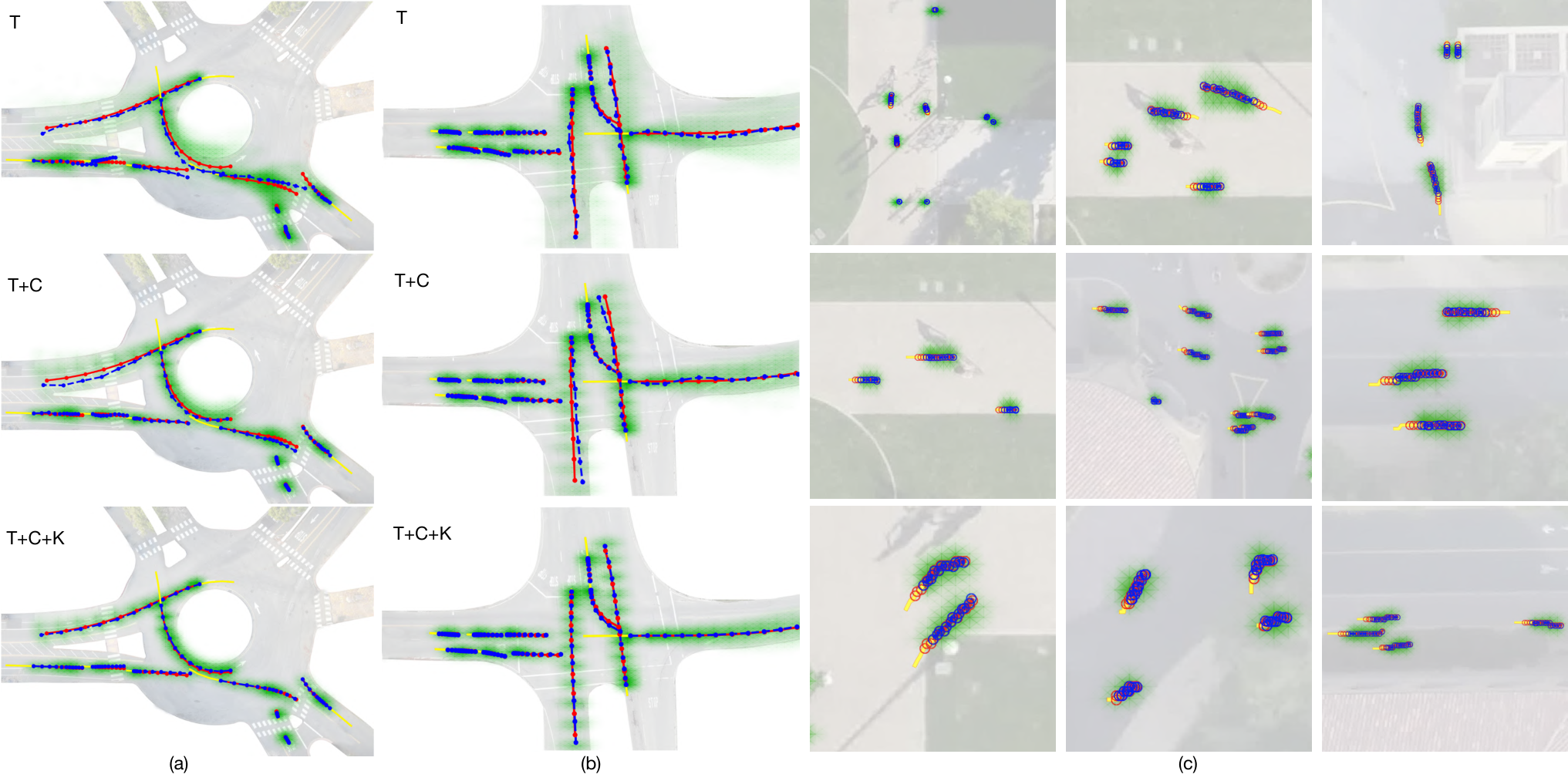
We qualitatively evaluated on prediction hypotheses of typical testing cases in Figure 4. Although we jointly predict all agents in a scene, we show predictions for a subset for simplicity. It shows that our approach can handle different challenging scenarios (e.g. intersection, roundabout) and diverse behaviors (e.g. going straight, turning, stopping) of vehicles and pedestrians. The ground truth is close to the mean of the predicted distribution and the model also allows for uncertainty.
We also conducted ablative analysis on the ID dataset to demonstrate relative significance of context information, double-attention mechanism and kinematic constraint layer in Social-WaGDAT. The ADE and FDE of each model setting are shown in the right part of Table 3.
versus : We show the effectiveness of employing scene context information. is the model without the kinematic layer, which only uses trajectory information, while further employs context information. The models directly output the position displacements at each step, which are aggregated to get complete trajectories. We can see little difference on prediction errors over short horizons while the gap becomes larger as the horizon extends. The reason is that the vehicle trajectories within a short period can be approximated by the constant velocity model, which are not heavily restricted or affected by the static context. However, as the forecasting horizon increases, the effects of context constraints cannot be ignored anymore, which leads to larger performance gain of leveraging context information. Compared with , the average prediction errors of are reduced by 11.1%, 10.1% and 2.6% in RA, UI and HR scenarios, respectively. This implies that the context information has larger effects on the prediction in RA and UI scenarios, where the influence of road geometries cannot be ignored. In Figure 4(a) and 4(b), the predicted distribution of is more compliant to roadways to avoid collisions and the vehicles near the “yield” or “stop” signs tend to yield or stop. However, generates samples that are outside of feasible areas and violating the traffic rules.
versus : We show the effectiveness of the proposed double-attention mechanism. uses equal attention coefficients in both topological and temporal layers. According to the statistics reported in Table 3, compared with equal attention, employing the double-attention mechanism to figure out relative importance within the topological structure and along different time steps can reduce the average prediction error by 20.1%, 13.9% and 10.5% in the RA, UI and HR scenarios, respectively. This implies that certain agents and periods have more significant influence than the rest.
versus : We show the effectiveness of the kinematic constraint layer. Employing the kinematic constraint layer to regularize the learning-based prediction hypotheses can further reduce the average prediction error by 20.6%, 12.3% and 3.1% in the RA, UI and HR scenarios, respectively. The reason is that due to the restriction from the kinematic model, unfeasible movements can be filtered out and the model is unlikely to overfit noisy data or outliers. Moreover, the improvement in RA and UI is more significant than in HR. The reason is that most vehicles go straight along the road in HR, whose behaviors can be well approximated by linear models. However, there are frequent turning behaviors in RA and UI which need constraints by more sophisticated models. We also visualize the predicted trajectories in Figure 4(a) and 4(b), where the ones with kinematic constraints are smoother and more plausible.
6 Conclusions
In this paper, we propose a generic system for multi-agent trajectory prediction named Social-WaGDAT, which considers both statistical context information, trajectories of interactive agents and physical feasibility constraints. In order to effectively model the interactions between different entities, we design a graph double-attention network to extract features from spatio-temporal dynamic graphs and a topological attention mechanism to figure out relative significance. Moreover, a variant of Wasserstein generative modeling is employed to support the whole framework. The Social-WaGDAT is validated by both pedestrian and vehicle trajectory prediction tasks. The experimental results show that our approach achieves smaller prediction error than multiple baseline methods. For the future work, we will consider the interactions between heterogeneous agents explicitly and jointly predict their trajectories.
References
- (1) Alexandre Alahi, Kratarth Goel, Vignesh Ramanathan, Alexandre Robicquet, Li Fei-Fei, and Silvio Savarese. Social lstm: Human trajectory prediction in crowded spaces. In Proceedings of the IEEE conference on computer vision and pattern recognition, pages 961–971, 2016.
- (2) Javad Amirian, Jean-Bernard Hayet, and Julien Pettré. Social ways: Learning multi-modal distributions of pedestrian trajectories with gans. In Proceedings of the IEEE Conference on Computer Vision and Pattern Recognition Workshops, pages 0–0, 2019.
- (3) Peter Battaglia, Razvan Pascanu, Matthew Lai, Danilo Jimenez Rezende, et al. Interaction networks for learning about objects, relations and physics. In Advances in neural information processing systems, pages 4502–4510, 2016.
- (4) Peter W Battaglia, Jessica B Hamrick, Victor Bapst, Alvaro Sanchez-Gonzalez, Vinicius Zambaldi, Mateusz Malinowski, Andrea Tacchetti, David Raposo, Adam Santoro, Ryan Faulkner, et al. Relational inductive biases, deep learning, and graph networks. arXiv preprint arXiv:1806.01261, 2018.
- (5) Yuning Chai, Benjamin Sapp, Mayank Bansal, and Dragomir Anguelov. Multipath: Multiple probabilistic anchor trajectory hypotheses for behavior prediction. arXiv preprint arXiv:1910.05449, 2019.
- (6) Chiho Choi and Behzad Dariush. Looking to relations for future trajectory forecast. arXiv preprint arXiv:1905.08855, 2019.
- (7) Nachiket Deo, Akshay Rangesh, and Mohan M Trivedi. How would surround vehicles move? a unified framework for maneuver classification and motion prediction. IEEE Transactions on Intelligent Vehicles, 3(2):129–140, 2018.
- (8) Nachiket Deo and Mohan M Trivedi. Convolutional social pooling for vehicle trajectory prediction. In Proceedings of the IEEE Conference on Computer Vision and Pattern Recognition Workshops, pages 1468–1476, 2018.
- (9) Tharindu Fernando, Simon Denman, Sridha Sridharan, and Clinton Fookes. Soft+ hardwired attention: An lstm framework for human trajectory prediction and abnormal event detection. Neural networks, 108:466–478, 2018.
- (10) Ian Goodfellow, Jean Pouget-Abadie, Mehdi Mirza, Bing Xu, David Warde-Farley, Sherjil Ozair, Aaron Courville, and Yoshua Bengio. Generative adversarial nets. In Advances in neural information processing systems, pages 2672–2680, 2014.
- (11) Agrim Gupta, Justin Johnson, Li Fei-Fei, Silvio Savarese, and Alexandre Alahi. Social gan: Socially acceptable trajectories with generative adversarial networks. In Proceedings of the IEEE Conference on Computer Vision and Pattern Recognition, pages 2255–2264, 2018.
- (12) Joey Hong, Benjamin Sapp, and James Philbin. Rules of the road: Predicting driving behavior with a convolutional model of semantic interactions. In Proceedings of the IEEE Conference on Computer Vision and Pattern Recognition, pages 8454–8462, 2019.
- (13) Xin Huang, Stephen G McGill, Brian C Williams, Luke Fletcher, and Guy Rosman. Uncertainty-aware driver trajectory prediction at urban intersections. In 2019 International Conference on Robotics and Automation (ICRA), pages 9718–9724. IEEE, 2019.
- (14) Ashesh Jain, Amir R Zamir, Silvio Savarese, and Ashutosh Saxena. Structural-rnn: Deep learning on spatio-temporal graphs. In Proceedings of the IEEE Conference on Computer Vision and Pattern Recognition, pages 5308–5317, 2016.
- (15) Dietmar Kasper, Galia Weidl, Thao Dang, Gabi Breuel, Andreas Tamke, Andreas Wedel, and Wolfgang Rosenstiel. Object-oriented bayesian networks for detection of lane change maneuvers. IEEE Intelligent Transportation Systems Magazine, 4(3):19–31, 2012.
- (16) Diederik P Kingma and Jimmy Ba. Adam: A method for stochastic optimization. arXiv preprint arXiv:1412.6980, 2014.
- (17) Diederik P Kingma and Max Welling. Auto-encoding variational bayes. arXiv preprint arXiv:1312.6114, 2013.
- (18) Jason Kong, Mark Pfeiffer, Georg Schildbach, and Francesco Borrelli. Kinematic and dynamic vehicle models for autonomous driving control design. In 2015 IEEE Intelligent Vehicles Symposium (IV), pages 1094–1099. IEEE, 2015.
- (19) Laura Leal-Taixé, Michele Fenzi, Alina Kuznetsova, Bodo Rosenhahn, and Silvio Savarese. Learning an image-based motion context for multiple people tracking. In Proceedings of the IEEE Conference on Computer Vision and Pattern Recognition, pages 3542–3549, 2014.
- (20) Namhoon Lee, Wongun Choi, Paul Vernaza, Christopher B Choy, Philip HS Torr, and Manmohan Chandraker. Desire: Distant future prediction in dynamic scenes with interacting agents. In Proceedings of the IEEE Conference on Computer Vision and Pattern Recognition, pages 336–345, 2017.
- (21) Stéphanie Lefèvre, Dizan Vasquez, and Christian Laugier. A survey on motion prediction and risk assessment for intelligent vehicles. ROBOMECH journal, 1(1):1, 2014.
- (22) Jiachen Li, Hengbo Ma, and Masayoshi Tomizuka. Interaction-aware multi-agent tracking and probabilistic behavior prediction via adversarial learning. In 2019 IEEE International Conference on Robotics and Automation (ICRA). IEEE, 2019.
- (23) Jiachen Li, Hengbo Ma, Wei Zhan, and Masayoshi Tomizuka. Generic probabilistic interactive situation recognition and prediction: From virtual to real. In 2018 21st International Conference on Intelligent Transportation Systems (ITSC), pages 3218–3224. IEEE, 2018.
- (24) Jiachen Li, Hengbo Ma, Wei Zhan, and Masayoshi Tomizuka. Conditional generative neural system for probabilistic trajectory prediction. In in 2019 IEEE/RSJ International Conference on Intelligent Robots and Systems (IROS). IEEE, 2019.
- (25) Zirui Li, Boyang Wang, Jianwei Gong, Tianyun Gao, Chao Lu, and Gang Wang. Development and evaluation of two learning-based personalized driver models for pure pursuit path-tracking behaviors. In 2018 IEEE Intelligent Vehicles Symposium (IV), pages 79–84. IEEE, 2018.
- (26) Junwei Liang, Lu Jiang, Juan Carlos Niebles, Alexander G Hauptmann, and Li Fei-Fei. Peeking into the future: Predicting future person activities and locations in videos. In Proceedings of the IEEE Conference on Computer Vision and Pattern Recognition, pages 5725–5734, 2019.
- (27) Zhouhan Lin, Minwei Feng, Cicero Nogueira dos Santos, Mo Yu, Bing Xiang, Bowen Zhou, and Yoshua Bengio. A structured self-attentive sentence embedding. arXiv preprint arXiv:1703.03130, 2017.
- (28) Wei Liu, Hongwen He, and Fengchun Sun. Vehicle state estimation based on minimum model error criterion combining with extended kalman filter. Journal of the Franklin Institute, 353(4):834–856, 2016.
- (29) Matthias Luber, Johannes A Stork, Gian Diego Tipaldi, and Kai O Arras. People tracking with human motion predictions from social forces. In IEEE ICRA, pages 464–469. IEEE, 2010.
- (30) Hengbo Ma, Jiachen Li, Wei Zhan, and Masayoshi Tomizuka. Wasserstein generative learning with kinematic constraints for probabilistic interactive driving behavior prediction. In 2019 IEEE Intelligent Vehicles Symposium (IV), pages 2477–2483. IEEE, 2019.
- (31) Yuexin Ma, Xinge Zhu, Sibo Zhang, Ruigang Yang, Wenping Wang, and Dinesh Manocha. Trafficpredict: Trajectory prediction for heterogeneous traffic-agents. In Proceedings of the AAAI Conference on Artificial Intelligence, volume 33, pages 6120–6127, 2019.
- (32) Stefano Pellegrini, Andreas Ess, and Luc Van Gool. Improving data association by joint modeling of pedestrian trajectories and groupings. In European conference on computer vision, pages 452–465. Springer, 2010.
- (33) Alexandre Robicquet, Amir Sadeghian, Alexandre Alahi, and Silvio Savarese. Learning social etiquette: Human trajectory understanding in crowded scenes. In ECCV, pages 549–565. Springer, 2016.
- (34) Andrey Rudenko, Luigi Palmieri, Michael Herman, Kris M Kitani, Dariu M Gavrila, and Kai O Arras. Human motion trajectory prediction: A survey. arXiv preprint arXiv:1905.06113, 2019.
- (35) Amir Sadeghian, Vineet Kosaraju, Ali Sadeghian, Noriaki Hirose, Hamid Rezatofighi, and Silvio Savarese. Sophie: An attentive gan for predicting paths compliant to social and physical constraints. In Proceedings of the IEEE Conference on Computer Vision and Pattern Recognition, pages 1349–1358, 2019.
- (36) Amir Sadeghian, Ferdinand Legros, Maxime Voisin, Ricky Vesel, Alexandre Alahi, and Silvio Savarese. Car-net: Clairvoyant attentive recurrent network. In Proceedings of the European Conference on Computer Vision (ECCV), pages 151–167, 2018.
- (37) Jacob Scharcanski, Alessandro Bof de Oliveira, Pablo G Cavalcanti, and Yessenia Yari. A particle-filtering approach for vehicular tracking adaptive to occlusions. IEEE Transactions on Vehicular Technology, 60(2):381–389, 2010.
- (38) Shan Su, Cheng Peng, Jianbo Shi, and Chiho Choi. Potential field: Interpretable and unified representation for trajectory prediction. arXiv preprint arXiv:1911.07414, 2019.
- (39) Liting Sun, Wei Zhan, and Masayoshi Tomizuka. Probabilistic prediction of interactive driving behavior via hierarchical inverse reinforcement learning. In 2018 21st International Conference on Intelligent Transportation Systems (ITSC), pages 2111–2117. IEEE, 2018.
- (40) Ilya Tolstikhin, Olivier Bousquet, Sylvain Gelly, and Bernhard Schoelkopf. Wasserstein auto-encoders. arXiv preprint arXiv:1711.01558, 2017.
- (41) Petar Veličković, Guillem Cucurull, Arantxa Casanova, Adriana Romero, Pietro Lio, and Yoshua Bengio. Graph attention networks. arXiv preprint arXiv:1710.10903, 2017.
- (42) Anirudh Vemula, Katharina Muelling, and Jean Oh. Social attention: Modeling attention in human crowds. In 2018 IEEE International Conference on Robotics and Automation (ICRA), pages 1–7. IEEE, 2018.
- (43) Wenshuo Wang, Junqiang Xi, and Ding Zhao. Learning and inferring a driver’s braking action in car-following scenarios. IEEE Transactions on Vehicular Technology, 67(5):3887–3899, 2018.
- (44) Xiaolong Wang, Ross Girshick, Abhinav Gupta, and Kaiming He. Non-local neural networks. In Proceedings of the IEEE Conference on Computer Vision and Pattern Recognition, pages 7794–7803, 2018.
- (45) Yanyu Xu, Zhixin Piao, and Shenghua Gao. Encoding crowd interaction with deep neural network for pedestrian trajectory prediction. In Proceedings of the IEEE Conference on Computer Vision and Pattern Recognition, pages 5275–5284, 2018.
- (46) Vinicius Zambaldi, David Raposo, Adam Santoro, Victor Bapst, Yujia Li, Igor Babuschkin, Karl Tuyls, David Reichert, Timothy Lillicrap, Edward Lockhart, et al. Relational deep reinforcement learning. arXiv preprint arXiv:1806.01830, 2018.
- (47) Wei Zhan, Liting Sun, Yeping Hu, Jiachen Li, and Masayoshi Tomizuka. Towards a fatality-aware benchmark of probabilistic reaction prediction in highly interactive driving scenarios. In 2018 21st International Conference on Intelligent Transportation Systems (ITSC), pages 3274–3280. IEEE, 2018.
- (48) Wei Zhan, Liting Sun, Di Wang, Haojie Shi, Aubrey Clausse, Maximilian Naumann, Julius Kümmerle, Hendrik Königshof, Christoph Stiller, Arnaud de La Fortelle, and Masayoshi Tomizuka. INTERACTION Dataset: An INTERnational, Adversarial and Cooperative moTION Dataset in Interactive Driving Scenarios with Semantic Maps. arXiv:1910.03088 [cs, eess], 2019.
- (49) Shengjia Zhao, Jiaming Song, and Stefano Ermon. Infovae: Information maximizing variational autoencoders. arXiv preprint arXiv:1706.02262, 2017.
- (50) Tianyang Zhao, Yifei Xu, Mathew Monfort, Wongun Choi, Chris Baker, Yibiao Zhao, Yizhou Wang, and Ying Nian Wu. Multi-agent tensor fusion for contextual trajectory prediction. In Proceedings of the IEEE Conference on Computer Vision and Pattern Recognition, pages 12126–12134, 2019.
7 Model Details
In this section, we introduce the implementation details of our model.
- •
Deep Feature Extractor (FE): The State MLP and Relation MLP both have three layers with 64 hidden units. The Context CNN consists of five layers with kernel size with zero paddings to keep the size of the image-like tensor.
- •
Graph Double-Attention Network (GDAT): The dimension of node attributes are 64 and the dimension of edge attributes is 16. These dimensions are fixed in different rounds of message passing. The activation functions in the attention mechanism are LeakyReLU.
- •
Encoding Function (MLP): The encoding function is a three-layer MLP with 128 hidden units. The dimension of latent variable is 32.
- •
Decoding Function: The decoding function is a recurrent layer of GRU cells with 128 hidden units.
8 Loss function
In this section, we provide a supplementary introduction of the loss function we used. In zhao2017infovae, they proposed a variation of VAE model which can maximize the mutual information between latent variable and observable variable. In our model, the original loss function is:
| (10) |
This loss function is a Lagrange function of the following optimization problem:
| (11) | ||||
| (12) |
We assume the distribution of decoder and is a standard normal distribution. We use Maximum Mean Discrepancy (MMD) to approximate , combining with the GNN, then we have
| (13) | ||||
where
| (14) | ||||
is the deep feature extractor and is the proposed graph double-attention network.
9 Data Preprocessing
We used a sequence of modules to preprocess the raw data, which are shown in Figure 5. The details are introduced below.
9.1 Global Context Information
In order to provide better global context information, we designed two different representations, namely occupancy density map and mean velocity field. By constructing such global contexts offline, we did decentralized localization for the corresponding target agent and obtained their local context information. The context information was used in both training and testing phases.
Occupancy Density Map The density map describes the normalized frequency distribution of all the agents’ locations. For a specific scene, we first split our map into a number of bin areas, which are squares. Without loss of generality, we denote this histogram as , and all the agents in different frames as a set , where is the agent index and is the frame index. We obtained the global representation of density by calculating , where are the indices of the histogram and is an indicator function which equals 1 if is located in the bin area indicated by index and 0 otherwise. Then we normalized this density map by dividing all bin values by the maximum value in the histogram and used this normalized histogram as our occupancy density map.
Mean Velocity Field Similarly, we also created a map of velocity field which contains square areas. We denote the whole map as and the bin item indexed by as . The is a two-dimensional vector representing the average speed along vertical and horizontal axes of all the agents in this area. Mathematically, and .
9.2 Localization
After obtaining the global context offline, our model utilized a decentralized method to do localization for each agent during training and testing. Given the location and the moving direction of the current agent at the current time step, we obtained the local context centered on this agent along its moving direction from the global context. Figure 6 provides an illustrative example.
10 Baseline Methods
In this section, we provide a more detailed introduction to the baseline methods used in our paper.
- •
Constant Velocity Model (CVM): A widely used linear kinematics model in vehicle tracking with an assumption of constant velocity. This model can also be generalized to forecasting trajectories for pedestrians.
- •
Linear Regression (LR): A linear predictor which minimizes the least square error over the historical trajectories.
- •
Probabilistic LSTM (P-LSTM) Jiachen_ICRA19: The model structure is the same as a vanilla LSTM. But a noise term sampled from the normal distribution is added in the input to incorporate uncertainty, which results in a probabilistic model.
- •
Social-Forces luber2010people: The model is based on the concepts developed in the cognitive and social science communities that describe individual and collective pedestrian dynamics.
- •
Social LSTM (S-LSTM) alahi2016social: The model encodes the trajectories with an LSTM layer whose hidden states serve as the input of a social pooling layer.
- •
Social GAN (S-GAN and S-GAN-P) gupta2018social: The model introduces generative adversarial learning scheme into S-LSTM to improve performance.
- •
Social Attention (S-ATT) vemula2018social: The model deals with spatio-temporal graphs with recurrent neural networks, which is based on the architecture of Structural-RNN jain2016structural.
- •
Clairvoyant attentive recurrent network (CAR-Net) sadeghian2018car: The model employs a physical attention module to capture agent-space interaction but without considering interactions among agents.
- •
Social-Ways amirian2019social: The model uses a generative adversarial network (Info-GAN) to sample plausible predictions for any agent in the scene.
- •
SoPhie sadeghian2019sophie: The model leverages both context images and trajectory information to generate paths compliant to social and physical constraints.
- •
DESIRE lee2017desire: The model is a deep stochastic inverse optimal control framework based on RNN encoders and decoders.