Gravitational waves from r-mode instability of massive young sub- and super-Chandrasekhar white dwarfs

We determine the r-mode instability windows in presence of shear viscosity due to electron-ion scattering and strong magnetic fields in rapidly rotating hot, ultramagnetized sub- and super-Chandrasekhar white dwarfs. Hence, it is necessary to consider the effects of radiation on the evolution of mode energy. This is expressed as the integral of the fluid perturbation (Lindblom1998; Lindblom1999),

where $\rho$ is the mean density profile of the star, $\delta\vec{v}$, $\delta p$, $\delta\Phi$ and $\delta\rho$ are perturbations in the velocity, pressure, gravitational potential and density due to oscillation of the mode respectively. The dissipative timescale of an r-mode is (Lindblom1998),

where, the index ’$i$’ refers to the various dissipative mechanisms, i.e., gravitational wave emissions, viscosity and magnetic braking.

To the lowest order of $\delta\vec{v}$ and $\delta\rho$ the expression for energy of the mode in Eq.(1) can be reduced to a one-dimensional integral (Lindblom1998; Vidana2012) in the small angular velocity limit

where, R is the radius of the white dwarf, $\alpha_{r}$ is the dimensionless amplitude of the mode, $\Omega$ is the angular velocity of the white dwarf and $\rho(r)$ is the radial dependence of the mass density. Since the expression of $(\frac{d\widetilde{E}}{dt})$ due to gravitational radiation (Thorne1980; Owen1998), shear viscosity (2Lindblom1999) and magnetic braking (Ho2000) are known, Eq.(2) can be used to evaluate the imaginary part of $\frac{1}{\tau}$. It can be written as

where $1/\tau_{GR}$, $1/\tau_{M}$ and $1/\tau_{SV}$ are the contributions from gravitational radiation, magnetic braking and shear viscosity, respectively, and are given by

where, G and c in Eq.(5) are the gravitational constant and velocity of light; $B_{s}$ and $I$ in Eq.(6) are the surface magnetic field and moment of inertia of the white dwarf and $\eta$ and $l$ in Eq.(7) are the shear viscosity coefficient and mode index respectively.

The dominant contribution to the shear viscosity in hot white dwarf interiors is from the scattering of electrons with the ion liquid. The fit to the shear viscosity coefficient is given by (2Lindblom1999; Na84)

where,

where all the quantities are given in CGS units and $T_{6}$ and $\rho_{6}$ are measured in $10^{6}$ K and $10^{6}$ $gcm^{-3}$. In order to have transparent visualisation of the role of angular velocity and temperature on various timescales, it is useful to factor them out by defining fiducial timescales. Thus, we define fiducial gravitational timescale $\widetilde{\tau}_{GR}$ such that (Lindblom1998; Lindblom2000),

and the fiducial magnetic braking timescale is given by,

where $\Omega_{0}=\sqrt{\pi G\bar{\rho}}$ and $\bar{\rho}=3M/4\pi R^{3}$ is the mean density of white dwarf having mass $M$ and radius $R$. Thus Eq.(4) becomes

For a given temperature and mode $l$ the equation for critical angular velocity $\Omega_{c}$ is obtained from the condition $\frac{1}{\tau(\Omega_{c},T)}=0$. At a given T and mode $l$, the equation for the critical velocity is a polynomial of order $l+1$ in $\Omega_{c}^{2}$ and thus each mode has its own characteristic $\Omega_{c}$. Since the smallest of these, i.e. $l=2$, is the dominant contributor, study is being done for this mode only. The critical angular velocity $\Omega_{c}$ in terms of $\Omega_{0}$ for this mode is obtained from the equation

Once the Equation of State (EoS) is ascertained, then all physical quantities necessary for the calculation of r-mode instability can be performed.

When the angular velocity of a white dwarf goes beyond the critical value $\Omega_{c}$, the instability of r-mode sets in and the star emits gravitational radiation which takes away the energy and angular momentum, resulting the star to spin down to the region of stability. The evolution of the angular velocity when the r-mode amplitude $\alpha_{r}$ reaches saturation ($d\alpha_{r}/dt=0$), as the angular momentum is radiated to infinity by gravitational radiation, is given by (Owen1998; Mu18)

where $Q=\frac{3\tilde{J}}{2\tilde{I}}$ and

We take a completely degenerate relativistic free electron gas at absolute zero. Due to Pauli’s exclusion principle, the electrons encounter a degeneracy pressure which keeps them moving and hence the total energy of the Fermi gas is greater than the single-electron ground state energies. Since this degeneracy pressure is non-zero even when the temperature is zero it is sufficient to stabilize a white dwarf star (a Fermi gas of electrons) against gravitational collapse.

The degeneracy pressure of the electron gas is given by

where $m_{e}$ is the electron rest mass, $v$ is the velocity of the electrons with momentum $\vec{p}$ and $n_{p}d^{3}p$ is the electron number density with momenta between $\vec{p}$ and $\vec{p}+d\vec{p}$. The factor $\frac{1}{3}$ accounts for the spatial isotropy of pressure. For electrons having spin $\frac{1}{2}$, degeneracy = 2, $n_{p}d^{3}p=\frac{8\pi p^{2}dp}{h^{3}}$ and hence number density $n_{e}$ is given by

where $p_{F}$ is the Fermi momentum of the electron gas, $x_{F}=\frac{p_{F}}{m_{e}c}$ is the dimensionless Fermi momentum and $\lambda_{e}=\frac{\hbar}{m_{e}c}$ is the electron Compton wavelength. The energy density of the electron gas $\varepsilon_{e}$ is given by

which can be integrated along with Eq.(19) to give

where

and

and for the total energy density $\varepsilon$ both electrons (with their kinetic and rest mass energies) and rest mass energies of atomic nuclei contribute, so that

Here $m_{n}$ and $m_{p}$ are the neutron and proton masses, respectively and $f$ is the number of neutrons per electron. Atomic nuclei contributes to the mass of white dwarf and the pressure is provided by the degenerate electron gas. Usually, white dwarf stars consist of helium, carbon, oxygen, etc., for which the mass number is approximately twice the atomic number and hence $f=1$. To be more accurate, one should also subtract $n_{e}(1+f)$ times the binding energy per nucleon from the rest mass energy of atomic nucleus. This binding energy correction term depends on the composition and its effects are insignificant, e.g. in case of a helium white dwarf star it is about 0.7$\%$ of the rest mass of nucleus, and hence it is ignored in the calculations.

Like the previous case, here also we consider a completely degenerate free relativistic electron gas at zero temperature but immersed in a strong background magnetic field. Electrons, being charged, are now Landau quantized. Landau quantization modifies the EoS, which, in turn, changes the thermodynamic quantities of the electron gas like pressure and energy density. The magnetic field energy density and pressure are also taken into consideration. The total matter and magnetic field pressure and energy density determines the stability and mass-radius relationships of ultramagnetized white dwarfs. It is to be noted that at the values of magnetic field strengths relevant for white dwarf interiors, protons are weakly Landau quantized. This is because the mass of proton being $\sim 1836$ times larger than the mass of electron the proton cyclotron energy is $\sim 1836$ times lesser than that of the electron for the same value of the magnetic field, and hence it is ignored.

In order to find the thermodynamic quantities of a magnetized electron gas at zero temperature, we need to calculate the energy spectrum and the density of states. The quantum dynamics of a charged particle in a constant magnetic field is described in many previous articles (e.g. Sokolov and Ternov (1968) (ST68), Landau and Lifshitz (1977) (LL77), Canuto and Ventura (1977) (CV77) Mészáros (1992) (Me92)). We assume a uniform magnetic field $B$ directed along the positive z-axis and consider the dynamics of a charged particle of charge $q$ and mass $m_{e}$. In classical electrodynamics, the particle moves in a circular trajectory with radius and angular frequency (cyclotron frequency) given by

where $v_{\perp}$ is the velocity of the particle transverse to the magnetic field direction. The Hamiltonian of the system is given by

where $\vec{B}=\nabla\times\vec{A}$ and $\vec{A}$ is the vector potential. The magnetic vector potential is given by

and therefore

Since the operator $y$ is absent, the operator $\hat{p}_{y}$ commutes with this Hamiltonian . Hence $\hat{p}_{y}$ can be replaced by its eigenvalue $\hbar k_{y}$. Using the expression for cyclotron frequency $\omega_{c}=\frac{qB}{m_{e}c}$ we get

The first two terms in Eq. (30) depict the Hamiltonian of a quantum harmonic oscillator with the potential minimum shifted in coordinate space by $x_{0}=\frac{\hbar k_{y}}{m_{e}\omega_{c}}$. Since coordinate translation of the oscillator potential leaves the energies unaffected, the energy eigenvalues can be written as

The set of quantum states with a particular value of the quantum number $n$ is called a Landau Level. Each Landau level is degenerate as the energy is independent of $k_{y}$. If periodic boundary condition is assumed $k_{y}$ can take values $k_{y}=\frac{2\pi N}{l_{y}}$ where $N$ is another integer and $l_{x},l_{y},l_{z}$ are the dimensions of the system considered. The values of $N$ are constrained by the fact that the centre of the oscillator force $x_{0}$ must physically lie within the system, $0\leq x_{0}\leq l_{x}$ which implies $0\leq N\leq\frac{l_{x}l_{y}m_{e}\omega_{c}}{2\pi\hbar}=\frac{qBl_{x}l_{y}}{hc}$. Applying this to electrons having charge $q=-|e|$ and spin $s$, the maximum number of particles in each Landau level per unit area is $\frac{|e|B(2s+1)}{hc}$. If we solve Schrödinger’s equation with z-component of spin angular momentum $s_{z}$ in a constant and uniform magnetic field in z-direction, then Eq.(31) modifies to

The spin degeneracy $g_{\nu}=1$ for the lowest Landau level ($\nu=0$) and $g_{\nu}=2$ (for $s_{z}=\pm\frac{1}{2}$) for higher Landau levels ($\nu\neq 0$).

For extremely strong magnetic fields such that $\hbar\omega_{c}\geq m_{e}c^{2}$ electrons become relativistic. In that case, solving the Dirac equation in a constant magnetic field (Lai91) gives the energy eigenvalues

where the dimensionless magnetic field defined as $B_{d}=B/B_{c}$ is introduced with $B_{c}$ given by $\hbar\omega_{c}=\hbar\frac{|e|B_{c}}{m_{e}c}=m_{e}c^{2}\Rightarrow B_{c}=\frac{m_{e}^{2}c^{3}}{|e|\hbar}=4.414\times 10^{13}$ gauss. The density of states at zero temperature can be written as

and hence the electronic number density is given by

where $p_{F}(\nu)$ is the Fermi momentum in the $\nu$th Landau level and $\nu_{m}$ is the highest Landau level index. The electron Fermi energy $E_{F}$ in the $\nu$th Landau level is given by

and $\nu_{m}$ can be found from the condition $[p_{F}(\nu)]^{2}\geq 0$ or

where $\epsilon_{Fmax}=\frac{E_{Fmax}}{m_{e}c^{2}}$ is the dimensionless maximum Fermi energy of electrons for fixed $B_{d}$ and $\nu_{m}$. Very weak magnetic fields ($B_{d}<<1$) give very large number of Landau levels which then forms a continuum. The maximum value of Landau level index, $\nu_{m}$, is taken to be the nearest lowest integer. In terms of a dimensionless Fermi momentum $x_{F}(\nu)=\frac{p_{F}(\nu)}{m_{e}c}$, Eqns.(35) and (36) may be written as

and

or

The electron energy density is given by

where

The degeneracy pressure of the magnetized electron gas is given by

where

and

We consider white dwarfs to be in thermal equilibrium. In the thermal steady state, the gravitational radiation pumps energy into the r-mode at a rate given by (Ma13; Mu19)

where

is the canonical angular momentum of the r-mode. We further assume that all of the energy emitted from the star is due to the r-mode dissipation inside the star which implies (Ma13)

where $\sigma$ is Stefan’s constant, $T_{eff}$ is the effective surface temperature and $L_{\gamma}$ is the thermal photon luminosity at the surface of the star. From Eqs.(47),(48) and (49), we get

We calculate the masses and radii of non-magnetized and magnetized white dwarfs using the Tolman-
Oppenheimer-Volkoff (TOV) equations. If one considers a very high central density for $f=1$ white dwarfs, one can asymptotically reach the Chandrasekhar mass limit. Beyond a density of $\sim 4.3\times 10^{11}$ $gcm^{-3}$, the neutron drip point (Ch15), neutron rich nuclei appear and with further increase of density the free neutron states start populating, and the phase consists of neutron rich nuclei in a lattice embedded in a sea of electron and neutron gas.

For magnetized white dwarfs we take the EoS with and without Landau quantization of electron gas. Instead of a constant magnetic field we take a density-dependent magnetic field profile to be consistent. We take the variation of magnetic field (Ba97) in the interior of a magnetized white dwarf to be

where $B_{d}$ is the dimensionless magnetic field at electron number density $n_{e}$, $B_{sd}$ is the dimensionless surface magnetic field, $n_{0}$ is the central electron number density ($n_{e}$(r=0)) and $B_{0}$, $\beta$ and $\gamma$ are constants. $B_{0}$ can be computed from Eq. (51) by fixing the surface and central magnetic field values. Constants $\beta=0.8$ and $\gamma=0.9$ are chosen to provide stable magnetized white dwarf equilibrium models. Once central and surface magnetic fields are fixed, the variations of its profile in the stellar interior do not affect the results significantly. Moreover, the maximum value of the magnetic field at the centre is kept at 10$B_{c}$ which is $4.414\times 10^{14}$ gauss, lower than the maximum limit prescribed by N. Chamel et al. (Ch13) and surface magnetic field strength $\sim 10^{9}$ gauss determined from observational data (Fe15; Ke13; Ke15). For Landau quantized EoS, we get stable super-Chandrasekhar white dwarf masses (Mu17).

Table-I shows variations of the masses and radii of non-magnetized white dwarfs with central electron number density $n_{e}$. Table-II shows the mass-radius relationship of magnetized white dwarfs with no Landau quantization of electrons with $n_{e}$ for central magnetic field strength $B_{d}(centre)=0.1$ and fixed surface field $B_{s}=10^{9}$ gauss. It is interesting to note that varying the central magnetic field strength from 0.1 to 10 produced no significant changes of masses and radii for non-Landau quantized white dwarfs from the non-magnetized ones at the same central electronic number density. Table-III shows the mass-radius relationship of magnetized white dwarfs with Landau quantization of electrons for the central electronic number density $\sim 5\times 10^{-6}$ $fm^{-3}$ (corresponding to the central density of the maximum mass of non-magnetized white dwarf) for $B_{d}(centre)=0.1,1,2,5,7,10$ and $B_{s}=10^{9}$ gauss. Slight variations of the central density is needed due to convergence of the magnetic field strength at the centre. In this case we get super-Chandrasekhar white dwarfs.

For the above mentioned configurations of white dwarfs, we calculate the r-mode instability windows from the fiducial timescales and solving for the critical angular frequency as a function of core temperature and surface magnetic field using Eq.(13). In Figs. 1, 2 and 3 we plot the reduced critical frequency as a function of temperature for non-magnetized, magnetized but not Landau quantized and magnetized and Landau quantized rapidly rotating hot sub- and super-Chandrasekhar white dwarfs of different masses respectively. In Fig. 4 we plot the r-mode instability windows of $1.3968M_{\odot}$ white dwarf for all the three cases to show explicitly the effects of Landau quantization and magnetic braking. Table-IV shows the mass, radius, central magnetic field and critical frequency at $10^{8}$ K of $1.3968M_{\odot}$, $2.0217M_{\odot}$ and $2.8997M_{\odot}$.

In Fig. 5 we plot the time evolution of rotational frequencies of hot white dwarfs by integrating Eq.(15). We take the initial spin frequency to be the Keplerian frequency $\nu_{K}=\frac{\Omega_{K}}{2\pi}\approx\frac{1}{2\pi}\sqrt{\frac{GM}{R^{3}}}=\frac{2}{\sqrt{3}}\nu_{0}$. We take the amplitude of r-mode $\alpha_{r}$ for $\Omega=\Omega_{0}$ and keep it constant for a star of given mass $M$ and radius $R$ as it does not vary much. We take the surface temperature $T_{eff}=10^{5}$ K. In Fig. 6 we plot the time dependence of spindown rates and in Fig. 7 we plot the dependence of spindown rate on frequency. In these figures we took the same constant mass of $1.3968M_{\odot}$ to show the effects of Landau quantization and magnetic braking and also two super-Chandrasekhar white dwarf masses of $2.0217M_{\odot}$ and $2.8997M_{\odot}$ to show the mass dependence.

From Figs. 1, 2 and 3 we see that hot massive rapidly rotating sub- and super-Chandrasekhar accreting white dwarfs have lower reduced critical frequencies and therefore have a high probability to dwell in r-mode instability region and thus emit gravitational radiation. The reduced critical frequencies are lower for heavier white dwarfs at the same temperature and magnetic field. This is because of the fact that the ratios ${|\widetilde{\tau_{GR}}|}/{\widetilde{\tau_{M}}}$ and ${|\widetilde{\tau_{GR}}|}/{\tau_{SV}}$ rapidly decrease with increase in mass (Mu18). For the same magnetic field and mass, ${\Omega_{c}}/{\Omega_{0}}\propto{T^{-1/3}}$. For the same mass Fig. 4 depicts the effects of magnetic braking and Landau quantization (EoS) on the r-mode instability region. From Fig. 4 we see that magnetic braking increases the r-mode instability regions of magnetized white dwarfs and Landau quantization of electrons added with magnetic braking increases the instability regions even more. At the same temperature, the critical frequency of a Landau quantized white dwarf is lower than that of a non-Landau quantized magnetized white dwarf which is again lower than that of a magnetized white dwarf (see Table-IV). Magnetic fields can maintain the oscillation mode and prevents damping. This makes massive super-Chandrasekhar white dwarfs more prone to gravitational wave emission from r-mode instability which can be detected in the near future.

From Figs. 5, 6 and 7 we conclude that the spindown and spindown rates are higher for magnetized white dwarfs than those of non-magnetized ones because of the fact that the ratio ${\widetilde{\tau_{M}}}/{|\widetilde{\tau_{GR}}|}\propto{B_{s}^{-2}}$ for a fixed mass. In the saturated phase of the r-mode at later times the magnetic braking timescale becomes less than the gravitational radiation timescale which makes magnetic braking the dominant spindown mechanism. There is no considerable effect of Landau quantization in the spindown and spindown rates.

The gravitational wave strain amplitude $h_{0}^{r-mode}$ from r-modes dominated by $l=m=2$ current quadrupole emission is given by (Ma13)

where $r$ is the distance of the white dwarf and $\omega_{r}=\frac{4}{3}\Omega$ is the angular frequency of the r-mode.

The expressions of $\alpha_{r}$ (Eq.(50)) and $h_{0}^{r-mode}$
(Eq.(52)) can be written as (Pa18)

and

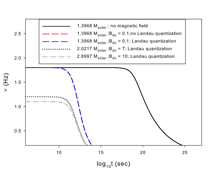
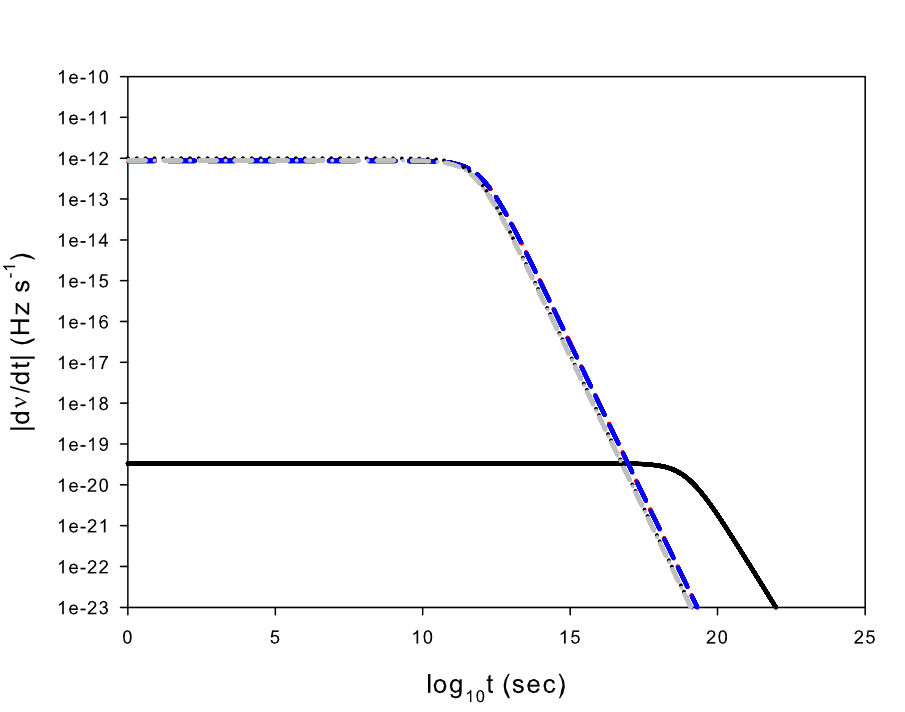
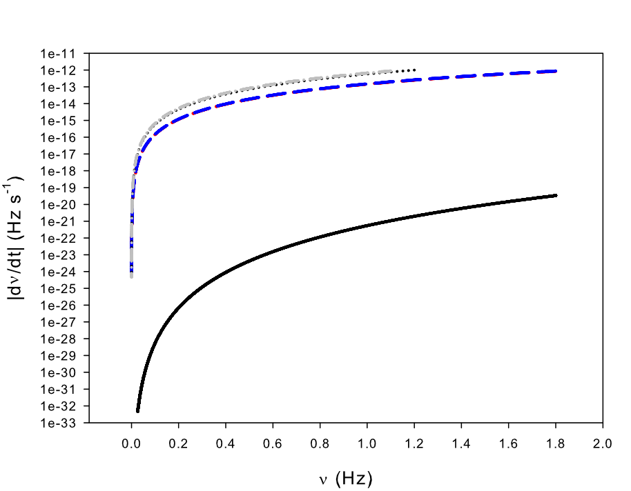
Table-V lists the strain amplitudes due to r-mode instability of sub- and super-Chandrasekhar white dwarfs at a distance of 1 kpc rotating at $\nu_{0}=\frac{\sqrt{3}}{2}\nu_{K}$. The masses and radii are the same as in Table-IV.

References

- (1) Kip S. Thorne and Alfonso Campolattaro 1967, Astrophys. J., 149, 591.
- (2) S. Chandrasekhar 1970, Phys. Rev. Lett., 24, 611.
- (3) J. L. Friedman and B. F. Schutz 1978, Astrophys. J., 222, 281.
- (4) Kostas Glampedakis and Leonardo Gualtieri 2018, The Physics and Astrophysics of Neutron Stars, Springer, 673-736.
- (5) U. Das and B. Mukhopadhyay 2012, Phys. Rev. D, 86, 042001.
- (6) U. Das and B. Mukhopadhyay 2013, Phys. Rev. Lett., 110, 071102.
- (7) Rajaram Nityananda and Sushan Konar 2014, Phys. Rev. D, 89, 103017.
- (8) Prasanta Bera and Dipankar Bhattacharya 2014, Mon. Not. R. Astron. Soc., 445, 3951.
- (9) D. Chatterjee, A. F. Fantina, N. Chamel, J. Novak and M. Oertel 2017, Mon. Not. R. Astron. Soc., 469, 95.
- (10) Somnath Mukhopadhyay, Debasis Atta and D. N. Basu 2017, Rom. Rep. Phys., 69, 101.
- (11) S. Chandrasekhar 1935, Mon. Not. R. Astron. Soc., 95, 207.
- (12) D. Andrew Howell et al. 2006, Nature, 443, 308.
- (13) R. A. Scalzo et al. 2010, Astrophys. J., 713, 1073.
- (14) M. Hicken et al. 2007, Astrophys. J. Lett., 669, L17.
- (15) M. Yamanaka et al. 2009, Astrophys. J. Lett., 707, L118.
- (16) Jeffrey M. Silverman et al. 2011, Mon. Not. R. Astron. Soc., 410, 1.
- (17) Manuel Malheiro, Jorge A. Rueda and Remo Ruffini 2012, Publ. Astron. Soc. Jpn., 64, 56.
- (18) Lilia Ferrario, Domitilla deMartino, Boris T. Gansicke 2015, arXiv: 1504.08072v1.
- (19) S. O. Kepler et. al. 2013, Mon. Not. R. Astron. Soc., 429, 2934.
- (20) S. O. Kepler et. al. 2015, Mon. Not. R. Astron. Soc., 446, 4078.
- (21) Nils Andersson, Kostas D. Kokkotas and Nikolaos Stergioulas 1999, Astrophys. J., 516, 307.
- (22) L. Lindblom, B. J. Owen, and S. M. Morsink 1998, Phys. Rev. Lett., 80, 4843.
- (23) L. Lindblom, G. Mendell, and B. J. Owen 1999, Phys. Rev. D, 60, 064006.
- (24) I. Vidaa 2012, Phys. Rev. C, 85, 045808.
- (25) K. S. Thorne 1980, Rev. Mod. Phys., 52, 299.
- (26) B. J. Owen, L. Lindblom, C. Cutler, B. F. Schutz, A. Vecchio, and N. Andersson 1998, Phys. Rev. D, 58, 084020.
- (27) L. Lindblom 1999, Phys. Rev. D, 60, 064007.
- (28) Wynn C. G. Ho and Dong Lai 2000, Astrophys. J., 543, 386.
- (29) R. Nandkumar and C. J. Pethick 1984, Mon. Not. R. Astron. Soc., 209, 511.
- (30) L. Lindblom, B. J. Owen, and G. Ushomirsky 2000, Phys. Rev. D, 62, 084030.
- (31) Somnath Mukhopadhyay, Joydev Lahiri, Debasis Atta, Kouser Imam and D. N. Basu 2018, Phys. Rev. C, 97, 065804.
- (32) A. A. Sokolov and I. M. Ternov 1968, Synchrotron Radiation, Pergamon, Oxford.
- (33) L. D. Landau and E. M. Lifshitz 1977, Quantum Mechanics 3rd. ed.; Pergamon, Oxford.
- (34) V. Canuto and J. Ventura 1977, Fundam. Cosmic Phys., 2, 203.
- (35) P. Mészáros 1992, High Energy Radiation from Magnetized Neutron Stars, University of Chicago, Chicago.
- (36) Dong Lai and Stuart L. Shapiro 1991, Astrophys. J., 383, 745.
- (37) Simin Mahmoodifar and Tod Strohmayer 2013, Astrophys. J., 773, 140.
- (38)
Sujan Roy, Somnath Mukhopadhyay, Joydev Lahiri,
Debasis Atta, Partha Roy Chowdhury and D. N. Basu 2019,arXiv:1905.06158v1. - (39) N. Chamel, Zh. K. Stoyanov, L. M. Mihailov, Y. D. Mutafchieva, R. L. Pavlov and Ch. J. Velchev 2015, Phys. Rev. C, 91, 065801.
- (40) D. Bandyopadhyay, S. Chakrabarty and S. Pal 1997, Phys. Rev. Lett., 79, 2176.
- (41) N. Chamel, A. F. Fantina and P. J. Davis 2013, Phys. Rev. D, 88, 081301 (R).
- (42) S. P. Pattnaik, T. R. Routray, X. Viñas, D. N. Basu, M. Centelles, K. Madhuri and B. Behera 2018, J. Phys. G, 45, 055202; S. P. Pattnaik, T. R. Routray, X. Viñas, D. N. Basu, M. Centelles, K. Madhuri and B. Behera 2018, J. Phys. G, 45, 119401.