Numerical relativity in spherical coordinates: A new dynamical spacetime and general relativistic MHD evolution framework for the Einstein Toolkit

I Introduction

II Basic Equations: Dynamical spacetime and GRMHD equations in spherical coordinates

III Implementation in the Einstein Toolkit

IV Code tests

V Conclusions and outlook

References

II.1 Spacetime evolution in spherical coordinates

II.2 GRMHD in the reference-metric formalism

II.3 Equations in orthonormal basis of spherical background metric

II.4 Evolution equations in integral form

IV.1 Tests in Minkowski spacetime

IV.2 Dynamical spacetime tests

II.2.1 Conservation laws in four-dimensional form

II.2.2 The 3+1 GRMHD equations in the reference-metric formalism

II.2.3 Vector potential evolution equations

II.2.4 Summary

IV.1.1 Relativistic spherical shock reflection test

IV.1.2 Spherical explosion

IV.2.1 Tilted, magnetized, uniformly rotating neutron star

IV.2.2 Collapse of a magnetized uniformly rotating neutron star

Abstract

pacs

Acknowledgements.

Vassilios Mewes Email: mewesv@ornl.gov Affiliation: National Center for Computational Sciences, Oak Ridge National Laboratory, P.O. Box 2008, Oak Ridge, TN 37831-6164, USA Affiliation: Physics Division, Oak Ridge National Laboratory, P.O. Box 2008, Oak Ridge, TN 37831-6354, USA Affiliation: Center for Computational Relativity and Gravitation, and School of Mathematical Sciences, Rochester Institute of Technology, 85 Lomb Memorial Drive, Rochester, New York 14623, USA Yosef Zlochower Affiliation: Center for Computational Relativity and Gravitation, and School of Mathematical Sciences, Rochester Institute of Technology, 85 Lomb Memorial Drive, Rochester, New York 14623, USA Manuela Campanelli Affiliation: Center for Computational Relativity and Gravitation, and School of Mathematical Sciences, Rochester Institute of Technology, 85 Lomb Memorial Drive, Rochester, New York 14623, USA Thomas W. Baumgarte Affiliation: Department of Physics and Astronomy, Bowdoin College, Brunswick, Maine 04011, USA Zachariah B. Etienne Affiliation: Department of Physics and Astronomy, West Virginia University, Morgantown, West Virginia 26506, USA Affiliation: Center for Gravitational Waves and Cosmology, West Virginia University, Chestnut Ridge Research Building, Morgantown, West Virginia 26505, USA Federico G. Lopez Armengol Affiliation: Center for Computational Relativity and Gravitation, and School of Mathematical Sciences, Rochester Institute of Technology, 85 Lomb Memorial Drive, Rochester, New York 14623, USA Affiliation: Instituto Argentino de Radioastronomía (IAR), C.C. No. 5, 1894 Buenos Aires, Argentina Federico Cipolletta Affiliation: INFN-TIFPA, Trento Institute for Fundamental Physics and Applications, Via Sommarive 14, I-38123 Trento, Italy Affiliation: Dipartimento di Fisica, Università di Trento, Via Sommarive 14, I-38123 Trento, Italy Affiliation: Center for Computational Relativity and Gravitation, and School of Mathematical Sciences, Rochester Institute of Technology, 85 Lomb Memorial Drive, Rochester, New York 14623, USA

We present SphericalNR, a new framework for the publicly available Einstein Toolkit that numerically solves the Einstein field equations coupled to the equations of general relativistic magnetohydrodynamics (GRMHD) in a 3+1 split of spacetime in spherical coordinates without symmetry assumptions. The spacetime evolution is performed using reference-metric versions of either the Baumgarte-Shapiro-Shibata-Nakamura equations or the fully covariant and conformal Z4 system with constraint damping. We have developed a reference-metric version of the Valencia formulation of GRMHD with a vector potential method, guaranteeing the absence of magnetic monopoles during the evolution. In our framework, every dynamical field (both spacetime and matter) is evolved using its components in an orthonormal basis with respect to the spherical reference-metric. Furthermore, all geometric information about the spherical coordinate system is encoded in source terms appearing in the evolution equations. This allows for the straightforward extension of Cartesian high-resolution shock-capturing finite volume codes to use spherical coordinates with our framework. To this end, we have adapted GRHydro, a Cartesian finite volume GRMHD code already available in the Einstein Toolkit, to use spherical coordinates. We present the full evolution equations of the framework, as well as details of its implementation in the Einstein Toolkit. We validate SphericalNR by demonstrating it passes a variety of challenging code tests in static and dynamical spacetimes.

04.25.D-, 04.30.-w, 04.70.Bw, 95.30.Sf, 97.60.Lf

The detection of gravitational waves (GW) from binary black hole (BBH) mergers via the ground-based LIGO and VIRGO detectors (Abbott et al. 2016a; Abbott et al. 2016b; Abbott et al. 2016c; Abbott et al. 2017a; Abbott et al. 2017b; Abbott et al. 2017c) and the simultaneous detection of GW and electromagnetic (EM) radiation from binary neutron star (BNS) mergers Abbott et al. 2017d; Abbott et al. 2017e; Abbott et al. 2017f has opened a new window into the Universe. Accurate numerical simulations of compact binary mergers are crucial for estimating the physical parameters of detected systems Aasi et al. 2014, and for informing physical models about the evolution of matter at nuclear densities in the postmerger remnant of BNSs and BHNSs Metzger 2017; Rosswog 2015. However, the full self-consistent numerical simulation of a compact object merger through coalescence and subsequent postmerger evolution at high resolution is an extremely challenging computational problem involving vast differences in length and timescales, as well as different approximate symmetries during the stages of the evolution. In particular, during the inspiral and merger, the absence of approximate axisymmetry lends itself to the use of Cartesian coordinates, while the postmerger remnant has approximate symmetries that are better captured by using spherical coordinates.

In the field of numerical relativity it is now possible to do self-consistent simulations of compact object binary mergers: The first general relativistic hydrodynamics (GRHD) BNS merger simulation Shibata and Uryū 2000, the breakthrough simulations of BBH mergers Pretorius 2005; Campanelli et al. 2006; Baker et al. 2006, the first GRHD black hole neutron star (BHNS) merger simulation Shibata and Uryū 2006, the first general relativistic magnetohydrodynamics (GRMHD) BNS merger simulations Anderson et al. 2008; Liu et al. 2008, and the first GRMHD simulation of BHNS mergers Chawla et al. 2010. Self-consistent simulations of these multimessenger sources requires the accurate modeling of the dynamical spacetime evolution and magnetohydrodynamic (MHD) flows within and near compact objects. To this end, many codes have been written that solve the equations of GRMHD. Generally such codes fall into two categories: GRMHD codes coupled to a 3+1 dynamical spacetime solver (see e.g. Shibata and Sekiguchi 2005; Duez et al. 2005; Antón et al. 2006; Anderson et al. 2006; Giacomazzo and Rezzolla 2007; Cerdá-Durán et al. 2008; Bucciantini and Del Zanna 2011; Mösta et al. 2014; Etienne et al. 2015; Dionysopoulou et al. 2013; Kidder et al. 2017; Hossein Nouri et al. 2018; Fambri et al. 2018; Cipolletta et al. 2019), and GRMHD codes that adopt analytical expressions for the spacetime geometry – which could be either exact, if the spacetime is stationary, or approximate for some dynamical spacetimes (see e.g. Koide et al. 1999; De Villiers and Hawley 2003; Gammie et al. 2003; Anninos et al. 2005; Komissarov 2004; Noble et al. 2006; Bonazzola et al. 2007; Noble et al. 2009; White et al. 2016; Porth et al. 2017; Liska et al. 2019). In general, the codes coupled to a 3+1 spacetime solver perform the fluid evolution on Cartesian or multipatch grids, while many of the fixed background spacetime codes employ curvilinear coordinates. A notable exception are the codes of Cerdá-Durán et al. 2008 and Bucciantini and Del Zanna 2011, which solve the fluid equations in curvilinear coordinates, coupled to a dynamical spacetime solver in an approximate, constrained evolution formulation of the Einstein field equations Cerdá-Durán et al. 2005; Cordero-Carrión et al. 2009; Cordero-Carrión et al. 2012, which is a generalization of the conformal flatness condition Wilson et al. 1996; Isenberg 2008.

Often, numerical error in conservation of momentum is smallest in the direction of coordinate lines. Accordingly, codes written in Cartesian coordinates conserve linear momentum well, while codes using spherical coordinates conserve angular momentum well. In GRMHD, momenta are only conserved when spacetime (rather than just coordinate) symmetries are present, due to the appearance of source terms in the evolution equations. Many astrophysical systems of interest to multimessenger astrophysics possess a natural axisymmetry at first approximation, so that one expects a better conservation of angular momentum in spherical coordinates, which allow the azimuthal coordinate to be aligned with the direction of this symmetry. Examples include (see references within the cited review articles): core-collapse supernovae Janka et al. 2007; Burrows 2013, compact binary merger remnants Shibata and Taniguchi 2011; Faber and Rasio 2012; Baiotti and Rezzolla 2017; Duez and Zlochower 2019; Radice et al. 2020, pulsars Lorimer 2005, magnetars Turolla et al. 2015; Mereghetti et al. 2015; Kaspi and Beloborodov 2017, and self-gravitating accretion disks Abramowicz and Fragile 2013. While there are techniques to mitigate the nonconservation of angular momentum in Cartesian coordinates (see e.g. Call et al. 2010; Mignone et al. 2012; Byerly et al. 2014), it would generally be more desirable to use numerical grids with spherical sampling, representing all tensors and vectors in the spherical basis. Evolving Einstein’s field equations in spherical coordinates introduces both conceptual and computational problems associated with coordinate singularities, but many of these issues have been resolved in recent years.

Among the formalisms of Einstein’s field equations most commonly used in numerical simulations is the Baumgarte-Shapiro-Shibata-Nakamura (BSSN) formulation Shibata and Nakamura 1995; Baumgarte and Shapiro 1999. Choices made in the original version of this formulation are suitable in Cartesian coordinates only, but a generalization involving a reference-metric formalism allows for applications in any coordinate system (see, e.g., Bonazzola et al. 2004; Shibata et al. 2004; Gourgoulhon 2007; Brown 2009; Montero and Cordero-Carrión 2012). In the absence of spherical symmetry, coordinate singularities can be handled by properly rescaling components of tensors Baumgarte et al. 2013; Montero et al. 2014; Baumgarte et al. 2015, which is equivalent to expressing all tensor components in a frame that is orthogonal with respect to the reference-metric. In Sanchis-Gual et al. 2014, the formalism was extended to the Z4 formalism (see, e.g., Bona et al. 2003; Bernuzzi and Hilditch 2010; Alic et al. 2012). The SENR/NRPy+ code Ruchlin et al. 2018 provides a flexible computational framework for the implementation of the formalism in a broad class of coordinate systems. Using this framework, we previously implemented this approach in the Einstein Toolkit Mewes et al. 2018.

In this work we extend the framework presented in Mewes et al. 2018 to evolve the GRMHD equations in a reference-metric formalism, and add a constraint-damping formulation for the spacetime evolution to the existing framework. Our new code applies this strategy by coupling the GRMHD equations with a fully dynamical spacetime evolution via the BSSN or fully covariant and conformal Z4 (fZZC4) system Sanchis-Gual et al. 2014 on three-dimensional spherical coordinate grids (i.e., no symmetry assumptions are made). The GRMHD evolution equations are evolved using a vector potential method. We also use the moving-puncture gauge conditions Campanelli et al. 2006; Baker et al. 2006. To our knowledge, SphericalNR is the first framework solving the coupled BSSN/fCCZ4 and GRMHD equations in three-dimensional spherical coordinate grids without symmetry assumptions.

The paper is organized as follows: In Sec. II, we describe the evolution equations for both spacetime and GRMHD in spherical coordinates. In Sec. III we describe the implementation of the GRMHD reference-metric evolution formalism in the Einstein Toolkit The Einstein Toolkit developers 2019. Code tests are presented in Sec. IV. Finally, Sec. V contains conclusions and discussions. Throughout this paper and in the code implementation we use geometrized and rationalized (geometrized Heaviside-Lorentz) units in which $c=G=M_{\odot}=\epsilon_{0}=\mu_{0}=1$ , where $c$ , $G$ , $M_{\odot}$ , $\epsilon_{0}$ , and $\mu_{0}$ are the speed of light, gravitational constant, solar mass, vacuum permittivity and vacuum permeability, respectively. Latin indices denote spatial indices, running from 1 to 3; Greek indices denote spacetime indices, running from 0 to 3 (0 is the time coordinate); and the Einstein summation convention is used.

We dynamically evolve the gravitational fields using a numerical relativity framework in spherical coordinates implemented using the Einstein Toolkit infrastructure (see Mewes et al. 2018). Our framework builds upon a reference-metric formulation Brown 2009; Gourgoulhon 2007; Montero and Cordero-Carrión 2012 of the BSSN formalism Nakamura et al. 1987; Shibata and Nakamura 1995; Baumgarte and Shapiro 1999. We appropriately scale out singular factors from components of tensors so that, for nonsingular spacetimes, all numerically evolved variables remain regular even at the origin and on the polar axis (see Baumgarte et al. 2013; Baumgarte et al. 2015). In this paper we extend the spacetime evolution code described in Mewes et al. 2018 to include the fCCZ4 formalism (see Sanchis-Gual et al. 2014), which applies the same reference-metric formalism and rescaling approach to the CCZ4 evolution equations Alic et al. 2012; Alic et al. 2013. This represents a conformal reformulation of the constraint-damped Z4 system (see Bona et al. 2003; Bona and Palenzuela 2004; Gundlach et al. 2005; see also Bernuzzi and Hilditch 2010 for an alternative conformal reformulation of Z4). We have now implemented the fCCZ4 formalism in the SphericalNR framework, and therefore provide, as a reference, key equations below.

The constraint-damped Z4 system Bona et al. 2003; Bona and Palenzuela 2004; Gundlach et al. 2005 replaces Einstein’s equations by

	$\displaystyle R_{\mu\nu}$	$\displaystyle+$	$\displaystyle\nabla_{\mu}\mathcal{Z}_{\nu}+\nabla_{\nu}\mathcal{Z}_{\mu}-\frac{\kappa_{1}}{\alpha}[n_{\mu}\mathcal{Z}_{\nu}+n_{\nu}\mathcal{Z}_{\mu}$		(1)
		$\displaystyle-$	$\displaystyle(1+\kappa_{2})g_{\mu\nu}n_{\lambda}\mathcal{Z}^{\lambda}]=8\pi(T_{\mu\nu}-\frac{1}{2}g_{\mu\nu}T),$		(1)

where $R_{\mu\nu}$ is the (spacetime) Ricci tensor, $g_{\mu\nu}$ the spacetime metric, $\nabla_{\mu}$ its associated covariant derivative, $T_{\mu\nu}$ the stress-energy tensor, $T\equiv g^{\mu\nu}T_{\mu\nu}$ its trace, $\mathcal{Z}_{\nu}$ a four-vector of constraints, and $\alpha$ the lapse function. We will shortly associate the timelike vector $n^{\mu}$ with the normal on spatial slices. Finally, $\kappa_{1}$ (units of inverse length) and $\kappa_{2}$ (dimensionless) are two damping coefficients, and all nonconstant constraint related modes are damped when $\kappa_{1}>0$ and $\kappa_{2}>-1$ Gundlach et al. 2005.

Following the discussion in Alic et al. 2013 regarding the stability of the evolution system in the presence of black holes (BH), we have redefined $\kappa_{1}\to\kappa_{1}/\alpha$ . The Z4 system reduces to the Einstein equations when the constraint vector $Z_{\mu}$ vanishes.

We start with a $3+1$ split of spacetime (see Darmois 1927) and foliate the four-dimensional spacetime with a set of nonintersecting spacelike hypersurfaces $\Sigma$ . We denote the future-pointing, timelike normal on $\Sigma$ as $n_{\mu}$ , and refer to the projection of the spacetime metric $g_{\mu\nu}$ onto $\Sigma$ as the spatial metric

\gamma_{\mu\nu}=g_{\mu\nu}+n_{\mu}n_{\nu}.

(2)

Expressing the normal vector in terms of a lapse function $\alpha$ and a shift vector $\beta^{i}$ ,

n^{\mu}=\left(\frac{1}{\alpha},-\frac{\beta^{i}}{\alpha}\right)

(3)

n_{\mu}=(-\alpha,0),

(4)

we may write the four-dimensional line element as

	$\displaystyle ds^{2}$	$\displaystyle=$	$\displaystyle g_{\mu\nu}dx^{\mu}dx^{\nu}$		(5)
		$\displaystyle=$	$\displaystyle-\alpha^{2}dt^{2}+\gamma_{ij}(dx^{i}+\beta^{i}dt)(dx^{j}+\beta^{j}dt),$		(5)

and the spacetime metric $g_{\mu\nu}$ as

g_{\mu\nu}=\left(\begin{array}[]{cc}-\alpha^{2}+\beta_{i}\beta^{i}&\beta_{j}\\ \beta_{i}&\gamma_{ij}\end{array}\right).

(6)

As in the BSSN formalism we conformally rescale the spatial metric according to

\bar{\gamma}_{ij}=e^{-4\phi}\gamma_{ij},

(7)

where $\bar{\gamma}_{ij}$ is the conformally related metric and $e^{\phi}$ the conformal factor. The latter can be written as

e^{4\phi}=(\gamma/\bar{\gamma})^{1/3},

(8)

where $\gamma$ and $\bar{\gamma}$ are the determinants of the physical and conformally related metric, respectively. We will assume that

\partial_{t}\bar{\gamma}=0,

(9)

meaning that $\bar{\gamma}$ remains equal to its initial value throughout the evolution. This choice, referred to as the “Lagrangian” choice in Brown 2009, simplifies some expressions in particular in the context of the GRMHD evolution, as explained below. We also rescale the trace-free part of the extrinsic curvature according to

\bar{A}_{ij}=e^{-4\phi}\left(K_{ij}-\frac{1}{3}\gamma_{ij}K\right),

(10)

where $K_{ij}$ is the physical extrinsic curvature and $K\equiv\gamma^{ij}K_{ij}$ its trace.

The central idea of the reference-metric formalism¹¹ 1 Splitting the metric into background and departures from the background (which need not to be small) is also done in bimetric formalisms Rosen 1963; Cornish 1964; Rosen 1973; Nahmad-Achar and Schutz 1987; Katz 1985; Katz et al. 1988; Katz and Ori 1990 in general relativity, in which reference-metrics are employed to give physical meaning to pseudotensors in curvilinear coordinates. We emphasize that we do not consider extensions of general relativity here; rather, we use the reference-metric only as a convenient approach to express Einstein’s equations (see also Gourgoulhon and Bonazzola 1994; Bonazzola et al. 2004; Shibata et al. 2004; Cook and Baumgarte 2008). is to express the conformally related metric as the sum of a background metric $\hat{\gamma}_{ij}$ and deviations $h_{ij}$ (which need not to be small),²² 2 Strictly speaking, it is sufficient to introduce a reference connection only (e.g. Brown 2009), but it is convenient to assume that this connection is associated with a reference-metric.

\bar{\gamma}_{ij}=\hat{\gamma}_{ij}+h_{ij}.

(11)

For our purposes it is particularly convenient to choose as the reference-metric the flat metric in spherical coordinates,

\hat{\gamma}_{ij}=\begin{pmatrix}1&0&0\\ 0&r^{2}&0\\ 0&0&r^{2}{\rm sin}^{2}\theta\end{pmatrix}.

(12)

Another key ingredient is evolving vector and tensor components in the orthonormal basis with respect to $\hat{\gamma}_{ij}$ instead of components in the spherical coordinate basis. To this end, we introduce a set of basis vectors $\hat{\mathbf{e}}^{\{k\}}_{i}$ that are orthonormal with respect to the background metric $\hat{\gamma}_{ij}$ :

\hat{\gamma}_{ij}=\delta_{\{k\}\{l\}}\hat{\mathbf{e}}^{\{k\}}_{i}\hat{\mathbf{e}}^{\{l\}}_{j}.

(13)

Since $\hat{\gamma}_{ij}$ is diagonal, the orthonormal vector basis tetrad and its inverse are given by

	$\displaystyle\hat{\mathbf{e}}^{\{k\}}_{i}$	$\displaystyle=\operatorname{diag}(1,r,r\sin\theta),$		(14)
	$\displaystyle\hat{\mathbf{e}}^{k}_{\{i\}}$	$\displaystyle=\operatorname{diag}(1,1/r,1/(r\sin\theta)),$		(15)

where we have adopted a notation involving plain Latin and Latin indices surrounded with curly braces: The components of a tensor ${\bf T}$ in the standard coordinate basis will be denoted using the former, while the tensor components in the background orthonormal basis will be denoted by the latter, respectively. In this notation, we may write the deviation tensor $h_{ij}$ as

h_{ij}=\hat{\mathbf{e}}^{\{k\}}_{i}\hat{\mathbf{e}}^{\{l\}}_{j}h_{\{k\}\{l\}}

(16)

and similarly write $\bar{A}_{ij}$ as³³ 3 This is a novel notation since, in standard references, different symbols are used for rescaled quantities. For instance, in Baumgarte et al. 2013, the pairs $\{h_{ij},h_{\{i\}\{j\}}\}$ , $\{\bar{A}_{ij},\bar{A}_{\{k\}\{l\}}\}$ are denoted as $\{\epsilon_{ij},h_{ij}\}$ , $\{\bar{A}_{ij},a_{ij}\}$ , respectively.

\bar{A}_{ij}=\hat{\mathbf{e}}^{\{k\}}_{i}\hat{\mathbf{e}}^{\{l\}}_{j}\bar{A}_{\{k\}\{l\}}.

(17)

While we will write most equations in terms of coordinate components (i.e. indices without curly braces), the code uses components in the orthogonal basis (i.e. with curly indices) as dynamical variables.

As in the original BSSN formalism, we introduce conformal connection functions $\bar{\Lambda}^{i}$ as independent variables. In the context of the reference-metric formalism the $\bar{\Lambda}^{i}$ satisfy the initial constraint

\bar{\Lambda}^{i}-\Delta\Gamma^{i}=0,

(18)

where

\Delta\Gamma^{i}\equiv\bar{\gamma}^{jk}\Delta\Gamma^{i}_{jk}

(19)

and

\Delta\Gamma^{i}_{jk}\equiv\bar{\Gamma}^{i}_{jk}-\hat{\Gamma}^{i}_{jk}.

(20)

Contrary to the Christoffel symbols themselves, differences between Christoffel symbols transform as rank-3 tensors. We compute the $\Delta\Gamma^{i}_{jk}$ from

	$\displaystyle\Delta\Gamma^{i}_{jk}$	$\displaystyle=\frac{1}{2}\bar{\gamma}^{il}\left(\hat{\mathcal{D}}_{j}\bar{\gamma}_{kl}+\hat{\mathcal{D}}_{k}\bar{\gamma}_{jl}-\hat{\mathcal{D}}_{l}\bar{\gamma}_{jk}\right)$
		$\displaystyle=\frac{1}{2}\bar{\gamma}^{il}\left(\hat{\mathcal{D}}_{j}h_{kl}+\hat{\mathcal{D}}_{k}h_{jl}-\hat{\mathcal{D}}_{l}h_{jk}\right),$		(21)

where $\hat{\mathcal{D}}_{i}$ is the covariant derivative associated with the reference-metric $\hat{\gamma}_{ij}$ , and where we have used $\hat{\mathcal{D}}_{i}\hat{\gamma}_{jk}=0$ in the second equality. Derivatives of coordinate components of tensors are evaluated by using the chain rule to analytically take derivatives of the basis vectors $\hat{\mathbf{e}}^{\{k\}}_{i}$ , while the orthonormal components are finite-differenced numerically in the code, e.g.

\partial_{k}h_{ij}=\hat{\mathbf{e}}^{\{l\}}_{i}\hat{\mathbf{e}}^{\{m\}}_{j}\partial_{k}h_{\{l\}\{m\}}+h_{\{l\}\{m\}}\partial_{k}\left(\hat{\mathbf{e}}^{\{l\}}_{i}\hat{\mathbf{e}}^{\{m\}}_{j}\right).

(22)

Similar to our treatment of the metric and extrinsic curvature we write

\bar{\Lambda}^{i}=\hat{\mathbf{e}}^{i}_{\{j\}}\bar{\Lambda}^{\{j\}}=\begin{pmatrix}\bar{\Lambda}^{\{r\}}\\ \bar{\Lambda}^{\{\theta\}}/r\\ \bar{\Lambda}^{\{\varphi\}}/(r\sin\theta)\end{pmatrix}

(23)

and evolve the orthonormal components $\bar{\Lambda}^{\{i\}}$ in our code.

One of the attractive features of the reference-metric formalism is that all quantities, including the conformal connection functions $\bar{\Lambda}^{i}$ , transform as tensor densities of weight zero⁴⁴ 4 A tensor density of weight $w$ acquires a power $J^{w}$ in a coordinate transformation, where $J\equiv\mathrm{det}|J^{i^{\prime}}_{j}|$ is the determinant of the Jacobian matrix of the coordinate transformation $J^{i^{\prime}}_{j}\equiv\frac{\partial x^{i^{\prime}}}{\partial x^{j}}$ . For example, a rank (2,0) tensor density of weight $w$ transforms as: $\mathcal{T}^{i^{\prime}j^{\prime}}=J^{w}J^{i^{\prime}}_{k}J^{j^{\prime}}_{l}\mathcal{T}^{kl}$ . Tensor densities of weight zero therefore transform as ordinary (or absolute) tensors with familiar coordinate transformations. (see Brown 2009).

We now extend the above formalism to the $Z4$ formulation, following Sanchis-Gual et al. 2014. We start with a 3+1 decomposition of the constraint vector $\mathcal{Z}_{\mu}$ ,

\mathcal{Z}_{\mu}=g_{\mu}^{~\nu}\mathcal{Z}_{\nu}=\gamma_{\mu}^{~\nu}\mathcal{Z}_{\nu}-n_{\mu}n^{\nu}\mathcal{Z}_{\nu},

(24)

and define

	$\displaystyle\Theta$	$\displaystyle\equiv$	$\displaystyle-n_{\lambda}\mathcal{Z}^{\lambda}=\alpha\mathcal{Z}^{0},$		(25)
	$\displaystyle Z_{i}$	$\displaystyle\equiv$	$\displaystyle\gamma_{i}^{\lambda}\mathcal{Z}_{\lambda}.$		(26)

In Eq. (29) below we will absorb the spatial parts $Z_{i}$ into the connection functions $\bar{\Lambda}^{i}$ , but we will evolve $\Theta$ as a new independent variable.

In order to write the evolution equations of the fCCZ4 system, we first define a new tensor

\bar{R}^{Z4}_{ij}\equiv\bar{R}_{ij}+\mathcal{D}_{i}Z_{j}+\mathcal{D}_{j}Z_{i},

(27)

where $\mathcal{D}_{i}$ is the covariant derivative associated with the spatial metric $\gamma_{ij}$ and $\bar{R}_{ij}$ is the Ricci tensor associated with the conformal metric $\bar{\gamma}_{ij}$ ,

	$\displaystyle\bar{R}_{ij}$	$\displaystyle=-\frac{1}{2}\bar{\gamma}^{kl}\hat{\mathcal{D}}_{k}\hat{\mathcal{D}}_{l}\bar{\gamma}_{ij}+\bar{\gamma}_{k(i}\hat{\mathcal{D}}_{j)}\Delta\Gamma^{k}+\Delta\Gamma^{k}\Delta\Gamma_{(ij)k}$
		$\displaystyle+\bar{\gamma}^{kl}(2\Delta\Gamma^{m}_{k(i}\Delta\Gamma_{j)ml}+\Delta\Gamma^{m}_{ik}\Delta\Gamma_{mjl}),$		(28)

where parentheses around indices indicate the symmetric part of a tensor: $T_{(ij)}\equiv\frac{1}{2}(T_{ij}+T_{ji})$ . We next define new conformal connection functions according to

\tilde{\Lambda}^{i}\equiv\Delta\Gamma^{i}+2\bar{\gamma}^{ij}Z_{j},

(29)

where we have used a tilde in order to distinguish these objects from $\bar{\Lambda}^{i}$ . We then have

Z^{i}=\frac{1}{2}e^{-4\phi}(\tilde{\Lambda}^{i}-\Delta\Gamma^{i}).

(30)

With these definitions, we may now write $R^{Z4}_{ij}$ as

$\displaystyle\bar{R}^{Z4}_{ij}=$	$\displaystyle-\frac{1}{2}\bar{\gamma}^{kl}\hat{\mathcal{D}}_{k}\hat{\mathcal{D}}_{l}\bar{\gamma}_{ij}$
	$\displaystyle+\bar{\gamma}_{k(i}\hat{\mathcal{D}}_{j)}(\tilde{\Lambda}^{k}-2e^{4\phi}Z^{k})+\mathcal{D}_{i}Z_{j}+\mathcal{D}_{j}Z_{i}$
	$\displaystyle+\Delta\Gamma^{k}\Delta\Gamma_{(ij)k}$
	$\displaystyle+\bar{\gamma}^{kl}(2\Delta\Gamma^{m}_{k(i}\Delta\Gamma_{j)ml}+\Delta\Gamma^{m}_{ik}\Delta\Gamma_{mjl}).$	(31)

Combining the terms $\bar{\gamma}_{k(i}\hat{\mathcal{D}}_{j)}(-2e^{4\phi}Z^{k})$ and $\mathcal{D}_{i}Z_{j}+\mathcal{D}_{j}Z_{i}$ it can be seen that all partial derivatives $\partial_{i}Z_{j}$ in $\bar{R}^{Z4}_{ij}$ cancel out exactly, meaning that $R^{Z4}_{ij}$ reduces to

\bar{R}^{Z4}_{ij}=\bar{R}_{ij}-8Z_{(i}\partial_{j)}\phi+2\gamma_{k(i}(\Gamma^{k}_{j)l}-\hat{\Gamma}^{k}_{j)l})Z^{l}.

(32)

With the above, and defining $\partial_{0}\equiv\partial_{t}-\mathcal{L}_{\beta}$ , where $\mathcal{L}_{\beta}$ is the Lie derivative along the shift $\beta^{i}$ , we arrive at the following set of coordinate basis evolution equations for the fCCZ4 system:

	$\displaystyle\partial_{0}\bar{\gamma}_{ij}$	$\displaystyle=-\frac{2}{3}\bar{\gamma}_{ij}\bar{\mathcal{D}}_{k}\beta^{k}-2\alpha\bar{A}_{ij},$
	$\displaystyle\partial_{0}\phi$	$\displaystyle=\frac{1}{6}\bar{\mathcal{D}}_{i}\beta^{i}-\frac{1}{6}\alpha K,$
	$\displaystyle\partial_{0}\bar{A}_{ij}$	$\displaystyle=-\frac{2}{3}\bar{A}_{ij}\bar{\mathcal{D}}_{k}\beta^{k}-2\alpha\bar{A}_{ik}\bar{A}^{k}_{j}+\alpha\bar{A}_{ij}(K-2\Theta)$
		$\displaystyle+e^{-4\phi}[-2\alpha\bar{\mathcal{D}}_{i}\bar{\mathcal{D}}_{j}\phi+4\alpha\bar{\mathcal{D}}_{i}\phi\bar{\mathcal{D}}_{j}\phi$
		$\displaystyle+4\bar{\mathcal{D}}_{(i}\alpha\bar{\mathcal{D}}_{j)}\phi-\bar{\mathcal{D}}_{i}\bar{\mathcal{D}}_{j}\alpha$
		$\displaystyle+\alpha(\bar{R}^{Z4}_{ij}-8\pi S_{ij})]^{\mathrm{TF}},$
	$\displaystyle\partial_{0}K$	$\displaystyle=e^{-4\phi}[\alpha(\bar{R}^{Z4}-8\bar{\mathcal{D}}^{i}\bar{\mathcal{D}}_{i}\phi-8\bar{\mathcal{D}}^{2}\phi)$
		$\displaystyle-(2\bar{\mathcal{D}}^{i}\alpha\bar{\mathcal{D}}_{i}\phi+\bar{\mathcal{D}}^{2}\alpha)]+\alpha(K^{2}-2\Theta K)$
		$\displaystyle-3\kappa_{1}(1+\kappa_{2})\Theta+4\pi\alpha(S-3E),$
	$\displaystyle\partial_{0}\Theta$	$\displaystyle=\frac{1}{2}\alpha[e^{-4\phi}(\bar{R}^{Z4}-8\bar{\mathcal{D}}^{i}\phi\bar{\mathcal{D}}_{i}\phi-8\bar{\mathcal{D}}^{2}\phi)$
		$\displaystyle-\bar{A}^{ij}\bar{A}_{ij}+\frac{2}{3}K^{2}-2\Theta K]$
		$\displaystyle-Z^{i}\partial_{i}\alpha-\kappa_{1}(2+\kappa_{2})\Theta-8\pi\alpha E,$
	$\displaystyle\partial_{0}\tilde{\Lambda}^{i}$	$\displaystyle=\bar{\gamma}^{jk}\hat{\mathcal{D}}_{j}\hat{\mathcal{D}}_{k}\beta^{i}+\frac{2}{3}\Delta\Gamma^{i}\bar{\mathcal{D}}_{j}\beta^{j}+\frac{1}{3}\bar{\mathcal{D}}^{i}\bar{\mathcal{D}}_{j}\beta^{j}$
		$\displaystyle-2\bar{A}^{jk}(\delta^{i}_{j}\partial_{k}\alpha-6\alpha\delta^{i}_{j}\partial_{k}\phi-\alpha\Delta\Gamma^{i}_{jk})$
		$\displaystyle-\frac{4}{3}\alpha\bar{\gamma}^{ij}\partial_{j}K+2\bar{\gamma}^{ij}(\alpha\partial_{j}\Theta-\Theta\partial_{j}\alpha)-\frac{4}{3}\alpha Ke^{4\phi}Z^{i}$
		$\displaystyle-2\kappa_{1}e^{4\phi}Z^{i}+2\kappa_{3}e^{4\phi}(\frac{2}{3}Z^{i}\hat{\mathcal{D}}_{k}\beta^{k}-Z^{k}\hat{\mathcal{D}}_{k}\beta^{i})$
		$\displaystyle-16\pi\alpha\bar{\gamma}^{ij}S_{j}.$

Here $[]^{\mathrm{TF}}$ denotes the trace-free part of a tensor: $T^{{\mathrm{TF}}}_{ij}\equiv T_{ij}-\frac{1}{3}\gamma_{ij}T^{k}_{~k}$ , and $\kappa_{3}$ is a constant that determines the covariance of the equations, in particular $\kappa_{3}=1$ (the choice adopted for all simulations presented in this work), corresponds to full covariance Alic et al. 2012. Unlike in Sanchis-Gual et al. 2014, we have absorbed all covariant derivatives of $Z^{i}$ in $\bar{R}^{Z4}_{ij}$ , meaning that no derivatives of the constraint vector appear in the above equations.

During the time evolution, we continuously enforce $\partial_{t}\bar{\gamma}=0$ , as well as the constraint $\bar{A}^{i}_{~i}=0$ . We have also implemented the $\chi=e^{4\phi}$ Campanelli et al. 2006 and $W=e^{2\phi}$ Marronetti et al. 2008 variants of the conformal factor evolution, resulting in the following evolution equations:

	$\displaystyle\partial_{0}\chi$	$\displaystyle=-\frac{2}{3}\chi\bar{\mathcal{D}}_{i}\beta^{i}+\frac{2}{3}\chi\alpha K,$		(33)
	$\displaystyle\partial_{0}W$	$\displaystyle=-\frac{1}{3}W\bar{\mathcal{D}}_{i}\beta^{i}+\frac{1}{3}W\alpha K.$		(34)

The choice between these variants can be made at runtime.

In order to close the evolution system we need to choose a gauge. For all dynamical spacetime evolution simulations presented in this paper we adopt the “standard gauge”, or “moving-puncture gauge”, meaning 1+log slicing

\partial_{t}\alpha=-2(K-2\Theta)+\beta^{i}\partial_{i}\alpha

(35)

for the lapse (see Bona et al. 1995) and a $\Gamma$ -driver⁵⁵ 5 The $\Gamma$ -driver owes its name to the appearance of the conformal connection functions $\tilde{\Gamma}^{i}$ introduced in Baumgarte and Shapiro 1999. While we use $\tilde{\Lambda}^{i}$ here, rather than $\tilde{\Gamma}^{i}$ , we still use the name $\Gamma$ -driver for this gauge condition.

	$\displaystyle\partial_{t}\beta^{i}$	$\displaystyle=$	$\displaystyle B^{i}+\beta^{j}\hat{\mathcal{D}}_{j}\beta^{i},$		(36)
	$\displaystyle\partial_{t}B^{i}$	$\displaystyle=$	$\displaystyle\frac{3}{4}(\partial_{t}\tilde{\Lambda}^{i}-\beta^{j}\hat{\mathcal{D}}_{j}\tilde{\Lambda}^{i})+\beta^{j}\hat{\mathcal{D}}_{j}B^{i}-\eta B^{i}$		(37)

for the shift (see Alcubierre et al. 2003). Here $\eta$ is a damping parameter with dimensions of inverse length, and we have adopted the covariant form of Brown 2009. In the code, the inclusion of shift advection terms can be turned off by the user at runtime.

As noted above, the actual evolved tensors in the code are not in the coordinate basis $\left\{\bar{\gamma}_{ij},\bar{A}_{ij},\tilde{\Lambda}^{i},\beta^{i},B^{i}=\dot{\beta}^{i}\right\}$ , but rather the orthonormal basis $\left\{h_{\{i\}\{j\}},\bar{A}_{\{i\}\{j\}},\tilde{\Lambda}^{\{i\}},\beta^{\{i\}},B^{\{i\}}=\dot{\beta}^{\{i\}}\right\}$ , respectively. The remaining evolved quantities $\left\{\alpha,K,\Theta,\phi\right\}$ are scalars and thus do not depend on choice of basis.

Finally, the matter sources in the spacetime evolution equations are given by projections of the stress-energy tensor, namely

$\displaystyle E$	$\displaystyle\equiv n^{\mu}n^{\nu}T_{\mu\nu}=\frac{1}{\alpha^{2}}\left(T_{tt}-2\beta^{i}T_{ti}+\beta^{i}\beta^{j}T_{ij}\right),$	(38)
$\displaystyle S_{i}$	$\displaystyle\equiv-\gamma_{i\mu}n_{\nu}T^{\mu\nu}=-\frac{1}{\alpha}T_{ti}+\frac{1}{\alpha}\beta^{j}T_{ij},$	(39)
$\displaystyle S_{ij}$	$\displaystyle\equiv\gamma_{i\mu}\gamma_{j\nu}T^{\mu\nu},$	(40)
$\displaystyle S$	$\displaystyle\equiv\gamma^{ij}S_{ij}.$	(41)

While we have only presented the fCCZ4 equations above, the user can select to evolve the BSSN system at runtime as well.

In this section we review the reference-metric formalism for GRHD presented in Montero et al. 2014; Baumgarte et al. 2015 and extend it to GRMHD, using a vector potential evolution scheme to guarantee the absence of magnetic monopoles.

The evolution of a magnetized fluid is governed by the conservation of baryon number

\nabla_{\mu}(\rho u^{\mu})=0,

(42)

which results in the continuity equation, and the conservation of energy-momentum

\nabla_{\mu}T^{\mu\nu}=\nabla_{\mu}(T^{\mu\nu}_{\mathrm{matter}}+T^{\mu\nu}_{\mathrm{EM}})=0,

(43)

which results in the (relativistic) Euler equation and the conservation of total energy. Assuming a perfect fluid, the fluid stress-energy tensor $T^{\mu\nu}_{\mathrm{matter}}$ is given by

T^{\mu\nu}_{\mathrm{matter}}=\rho hu^{\mu}u^{\nu}+Pg^{\mu\nu},

(44)

where $\rho$ is the rest mass density, $P$ the fluid pressure, $h=1+\epsilon+P/\rho$ the specific enthalpy, $\epsilon$ the internal energy density, and $u^{\mu}$ the fluid four-velocity, respectively.

In terms of the Faraday tensor $F^{\mu\nu}$ , the EM stress-energy tensor is ⁶⁶ 6 The Heaviside-Lorentz (HL) units we adopt in this work are rationalized, as no explicit factors of $4\pi$ appear in the Maxwell equations in these units. Electric and magnetic fields in HL and Gauss units are therefore related by a factor of $\sqrt{4\pi}$ : $E^{\mu}_{\mathrm{[Gauss]}}=\sqrt{4\pi}E^{\mu}_{\mathrm{[HL]}}$ , $B^{\mu}_{\mathrm{[Gauss]}}=\sqrt{4\pi}B^{\mu}_{\mathrm{[HL]}}$ . Consequently, in Gauss units, the EM stress-energy tensor is defined as $T^{\mu\nu}_{\mathrm{EM}}=\frac{1}{4\pi}(F^{\mu\lambda}F^{\nu}_{\lambda}-\frac{1}{4}g^{\mu\nu}F^{\lambda\kappa}F_{\lambda\kappa})_{[\mathrm{Gauss}]}.$

T^{\mu\nu}_{\mathrm{EM}}=F^{\mu\lambda}F^{\nu}_{\lambda}-\frac{1}{4}g^{\mu\nu}F^{\lambda\kappa}F_{\lambda\kappa}.

(45)

We next decompose the Faraday tensor $F^{\mu\nu}$ as

F^{\mu\nu}=U^{\mu}E^{\nu}_{(U)}-U^{\nu}E^{\mu}_{(U)}+\epsilon^{\mu\nu\lambda\kappa}U_{\lambda}B_{\kappa(U)},

(46)

where

\epsilon^{\mu\nu\lambda\kappa}\equiv\frac{-1}{\sqrt{-g}}[\mu\nu\lambda\kappa],

(47)

and where $[\mu\nu\lambda\kappa]$ is the totally antisymmetric Levi-Civita symbol ( $=+(-)1$ for even (odd) permutations of $[0123]$ , and 0 if any two indices are repeated). Here $E^{\mu}_{(U)}$ and $B^{\mu}_{(U)}$ are the electric and magnetic fields measured by an observer with generic four-velocity $U^{\mu}$ ,

E^{\mu}_{(U)}=F^{\mu\nu}U_{\nu},\qquad B^{\mu}_{(U)}=\frac{1}{2}\epsilon^{\mu\nu\kappa\rho}U_{\nu}F_{\rho\kappa}.

(48)

Both $E^{\mu}_{(U)}$ and $B^{\mu}_{(U)}$ are orthogonal to $U^{\mu}$ , i.e. $E^{\mu}_{(U)}U_{\mu}=B^{\mu}_{(U)}U_{\mu}=0$ .

In the following we focus on two observers of particular interest, namely observers comoving with the fluid (i.e., with four-velocity $U^{\mu}=u^{\mu}$ ) and normal observers (with four-velocity $U^{\mu}=n^{\mu}$ ). Following convention, we denote the fields observed by the former with $E^{\mu}_{(u)}$ and $B^{\mu}_{(u)}$ , but the latter simply with $E^{\mu}=E^{\mu}_{(n)}$ and $B^{\mu}=B^{\mu}_{(n)}$ .

In the ideal MHD limit we assume that the fluid acts as a perfect conductor, meaning that the electric field observed by an observer comoving with the fluid vanishes:

E^{\mu}_{(u)}=F^{\mu\nu}u_{\nu}=0.

(49)

Thus in this approximation $F^{\mu\nu}$ , which generally depends on both electric and magnetic fields, can be expressed in terms of magnetic fields alone,

F^{\mu\nu}=\epsilon^{\mu\nu\lambda\kappa}u_{\lambda}B_{\kappa}^{(u)},

(50)

and ${}^{*}F^{\mu\nu}$ , the dual of the Faraday tensor, as

^{*}F^{\mu\nu}=\frac{1}{2}\epsilon^{\mu\nu\lambda\kappa}F_{\lambda\kappa}=u^{\mu}B_{(u)}^{\nu}-u^{\nu}B_{(u)}^{\mu}.

(51)

In the ideal MHD limit we can also write the magnetic field $B^{\mu}_{(u)}$ as a projection of $B^{\mu}$ along the fluid four-velocity $u^{\nu}$ ,

B^{\mu}_{(u)}=\frac{1}{W}P^{\mu}_{~\nu}B^{\nu},

(52)

where $P^{\mu}_{~\nu}=g^{\mu}_{~\nu}+u^{\mu}u_{\nu}$ , and where we have introduced the Lorentz factor $W$ between the fluid and normal observers, $W\equiv-n_{\mu}u^{\mu}=\alpha u^{t}$ . Inserting (52) into (51) yields

^{*}F^{\mu\nu}=\frac{1}{W}\left(u^{\mu}B^{\nu}-u^{\nu}B^{\mu}\right).

(53)

Introducing the abbreviation⁷⁷ 7 Similarly to differences in the EM stress-energy tensor, treatments that adopt Gauss units (De Villiers and Hawley 2003; Duez et al. 2005; Anninos et al. 2005; Bonazzola et al. 2007; Etienne et al. 2015) rather than Lorentz-Heaviside units (Koide et al. 1999; Gammie et al. 2003; Komissarov 2004; Shibata and Sekiguchi 2005; Antón et al. 2006; Anderson et al. 2006; Noble et al. 2006; Giacomazzo and Rezzolla 2007; Cerdá-Durán et al. 2008; Noble et al. 2009; Bucciantini and Del Zanna 2011; Dionysopoulou et al. 2013; Mösta et al. 2014; White et al. 2016; Kidder et al. 2017; Porth et al. 2017; Hossein Nouri et al. 2018; Fambri et al. 2018; Cipolletta et al. 2019; Liska et al. 2019) often use the definition $b^{\mu}\equiv B^{\mu}_{(u)}/\sqrt{4\pi}$ instead of (54). The resulting fields $b^{\mu}$ , however, are again identical in both treatments, so that expressions for the stress-energy tensor, for example, take the same from when written in terms of $b^{\mu}$ , see (55).

b^{\mu}\equiv B^{\mu}_{(u)}

(54)

we can write the electromagnetic stress-energy tensor as

T^{\mu\nu}_{\mathrm{EM}}=\left(u^{\mu}u^{\nu}+\frac{1}{2}g^{\mu\nu}\right)b^{2}-b^{\mu}b^{\nu},

(55)

where $b^{2}\equiv b^{\mu}b_{\mu}$ ; so that the total stress-energy tensor $T^{\mu\nu}$ becomes

T^{\mu\nu}=\rho\,h^{*}u^{\mu}u^{\nu}+P^{*}g^{\mu\nu}-b^{\mu}b^{\nu}.

(56)

Here we have defined $h^{*}=1+\epsilon+(P+b^{2})/\rho$ as the magnetically modified specific enthalpy and $P^{*}=P+b^{2}/2$ as the magnetically modified isotropic pressure. Finally, the evolution of the magnetic field is governed by the homogeneous Maxwell equations

\nabla_{\nu}(^{*}F^{\mu\nu})=0.

(57)

We now recast the above conservation laws using both a 3+1 split and a reference-metric approach. The result will be a set of equations that is suitable for numerical integration in spherical coordinates, and that meshes well with the form of the field equations as presented in Sec. II.1. The fluid equations have been previously derived in Montero et al. 2014; Baumgarte et al. 2015, and we will extend the formalism to the GRMHD equations.

The key idea is to repeatedly use identities for divergences (see, e.g., Problem 7.7 in Lightman et al. 1975). For the continuity equation (42), for example, we use

\nabla_{\nu}V^{\nu}=\frac{1}{\sqrt{|g|}}\partial_{\nu}(\sqrt{|g|}V^{\nu})

(58)

to arrive at

$\displaystyle 0$	$\displaystyle=\nabla_{\nu}(\rho u^{\nu})=\frac{1}{\sqrt{-g}}\partial_{\nu}(\sqrt{-g}\rho u^{\nu})$
	$\displaystyle=\frac{1}{\sqrt{-g}}\left(\partial_{t}(\sqrt{-g}\rho u^{t})+\partial_{i}(\sqrt{-g}\rho u^{i})\right)$
	$\displaystyle=\partial_{t}(e^{6\phi}\sqrt{\bar{\gamma}}\rho W)+\partial_{i}\left(\alpha e^{6\phi}\sqrt{\bar{\gamma}}\rho W\bar{v}^{i}\right).$	(59)

Here we have defined

v^{i}\equiv\frac{1}{W}\gamma^{i}_{~\nu}u^{\nu}=\frac{u^{i}}{W}+\frac{\beta^{i}}{\alpha}

(60)

as the fluid three-velocity and

\bar{v}^{i}\equiv v^{i}-\frac{\beta^{i}}{\alpha}=\frac{u^{i}}{W}

(61)

as the “advection velocity”. We have also written the square root of the determinant of the spacetime metric $\sqrt{-g}$ as

\sqrt{-g}=\alpha\sqrt{\gamma}=\alpha e^{6\phi}\sqrt{\bar{\gamma}}.

(62)

Equation (II.2.2) is the continuity equation in a form that is often referred to as the “Valencia” form of the equations (see Banyuls et al. 1997). This version of the equations is well suited for simulations in Cartesian coordinates, but in curvilinear coordinates the vanishing of the determinant $\bar{\gamma}$ may cause numerical problems. Following Montero et al. 2014, we apply the identity (58) again, and convert the partial derivatives $\partial_{i}$ to covariant derivatives $\hat{\mathcal{D}}_{i}$ associated with the background (reference) metric $\hat{\gamma}_{ij}$ ,⁸⁸ 8 We will assume throughout that the reference-metric $\hat{\gamma}_{ij}$ is independent of time.

0=\partial_{t}(e^{6\phi}\sqrt{\bar{\gamma}/\hat{\gamma}}\rho W)+\hat{\mathcal{D}}_{i}(\alpha e^{6\phi}\sqrt{\bar{\gamma}/\hat{\gamma}}\,\rho W\bar{v}^{i}).

(63)

Note that the combination $\bar{\gamma}/\hat{\gamma}$ remains finite for regular spacetimes. We now define the conserved density $D$

D\equiv e^{6\phi}\sqrt{\bar{\gamma}/\hat{\gamma}}\rho W

(64)

and the conserved density flux $f_{D}$

(f_{D})^{i}\equiv\alpha D\,\bar{v}^{i}

(65)

to write the continuity equation in the form

\partial_{t}D+\hat{\mathcal{D}}_{i}(f_{D})^{i}=0.

(66)

We note that a similar strategy is followed in the CoCoNuT code, without explicitly mentioning the reference-metric (see e.g. Dimmelmeier 2001). For reasons that will become apparent in Sec. II.4 below, we will implement the equation numerically as:

\partial_{t}D+\partial_{i}(f_{D})^{i}=-(f_{D})^{i}\hat{\Gamma}^{j}_{ij}.

(67)

We proceed similarly for the conservation of stress energy (43), except that we now use the identity

\nabla_{\lambda}T^{\lambda}_{\mu}=\frac{1}{\sqrt{|g|}}\partial_{\lambda}(\sqrt{|g|}T^{\lambda}_{\mu})-T^{\lambda}_{\sigma}\Gamma^{\sigma}_{\lambda\mu}

(68)

twice. The spatial projection of (43) then yields the relativistic Euler equation

\partial_{t}S_{j}+\hat{\mathcal{D}}_{i}(f_{S})_{j}^{i}=(s_{S})_{j}

(69)

\partial_{t}S_{j}+\partial_{i}(f_{S})_{j}^{i}=(s_{S})_{j}-(f_{S})_{j}^{i}\hat{\Gamma}^{k}_{ik}+(f_{S})^{i}_{k}\hat{\Gamma}^{k}_{ij},

(70)

where we have defined the conserved momentum

S_{j}\equiv e^{6\phi}\sqrt{\bar{\gamma}/\hat{\gamma}}T^{i}_{j}=e^{6\phi}\sqrt{\bar{\gamma}/\hat{\gamma}}(\rho h^{*}W^{2}v_{j}-\alpha b^{0}b_{j}),

(71)

the conserved momentum density fluxes

(f_{S})_{j}^{i}\equiv\alpha(S_{j}\bar{v}^{i}+e^{6\phi}\sqrt{\bar{\gamma}/\hat{\gamma}}\,P^{*}\delta^{i}_{j}-e^{6\phi}\sqrt{\bar{\gamma}/\hat{\gamma}}\,b_{j}B^{i}/W),

(72)

and where the source term is given by

	$\displaystyle(s_{S})_{j}$	$\displaystyle=\alpha e^{6\phi}\sqrt{\bar{\gamma}/\hat{\gamma}}\left(-T^{00}\alpha\partial_{j}\alpha+T^{0}_{i}\hat{\mathcal{D}}_{j}\beta^{i}\right.$
		$\displaystyle\left.+\frac{1}{2}(T^{00}\beta^{i}\beta^{k}+2T^{0i}\beta^{k}+T^{ik})\hat{\mathcal{D}}_{j}\gamma_{ik}\vphantom{\int_{1}^{2}}\right)$		(73)

(see Montero et al. 2014 for a detailed derivation). The terms $\hat{\mathcal{D}}_{j}\gamma_{ik}$ can be evaluated from

\hat{\mathcal{D}}_{j}\gamma_{ik}=e^{4\phi}(4\bar{\gamma}_{ik}\partial_{j}\phi+\hat{\mathcal{D}}_{j}\bar{\gamma}_{ik}),

(74)

where the $\hat{\mathcal{D}}_{j}\bar{\gamma}_{ik}=\hat{\mathcal{D}}_{j}h_{ik}$ are computed already in (II.1).

Projecting the conservation of stress energy (43) along $n_{\nu}$ and subtracting the continuity Eq. (42) yields

\nabla_{\mu}\left(n_{\nu}T^{\nu\mu}-\rho u^{\mu}\right)=T^{\mu\nu}\nabla_{\nu}n_{\mu}.

(75)

We again apply the identity (58) twice to arrive at the energy equation

\partial_{t}\tau+\hat{\mathcal{D}}_{i}(f_{\tau})^{i}=s_{\tau}

(76)

\partial_{t}\tau+\partial_{i}(f_{\tau})^{i}=s_{\tau}-(f_{\tau})^{i}\hat{\Gamma}^{j}_{ij},

(77)

where we have defined $\tau$ as the total conserved energy density subtracting the conserved density $D$ ⁹⁹ 9 The motivation to subtract the continuity equation from the projection of the stress-energy conservation along $n_{\mu}$ (75) was to arrive at an evolution for $\tau$ : It correctly recovers the Newtonian limit and is numerically more accurate than evolving the total conserved energy density (see e.g. Antón et al. 2006; Baumgarte and Shapiro 2010; Rezzolla and Zanotti 2013).:

\tau\equiv e^{6\phi}\sqrt{\bar{\gamma}/\hat{\gamma}}(\rho h^{*}W^{2}-P^{*}-(\alpha b^{0})^{2})-D,

(78)

the conserved energy flux

(f_{\tau})^{i}\equiv\alpha(\tau\bar{v}^{i}+e^{6\phi}\sqrt{\bar{\gamma}/\hat{\gamma}}\,P^{*}v^{i}-\alpha e^{6\phi}\sqrt{\bar{\gamma}/\hat{\gamma}}\,b^{0}B^{i}/W),

(79)

and where the source term is given by Montero et al. 2014

	$\displaystyle s_{\tau}$	$\displaystyle=\alpha e^{6\phi}\sqrt{\bar{\gamma}/\hat{\gamma}}(T^{00}(\beta^{i}\beta^{j}K_{ij}-\beta^{i}\partial_{i}\alpha)$
		$\displaystyle+T^{0i}(2\beta^{j}K_{ij}-\partial_{i}\alpha)+T^{ij}K_{ij}).$		(80)

In the above equations, both $B^{i}$ and $b^{\mu}=B^{\mu}_{(u)}$ make an appearance. The two fields are related by (52), so that we can always compute $B^{\mu}_{(u)}$ from $B^{\mu}$ . Specifically, we contract (52) with $n_{\mu}$ to obtain

b^{0}=\frac{WB^{i}v_{i}}{\alpha},

(81)

while a spatial projection of (52) yields

b^{i}=\frac{B^{i}}{W}+W(B^{j}v_{j})\bar{v}^{i}.

(82)

We also have

b^{2}=\frac{B^{i}B_{i}}{W^{2}}+(B^{i}v_{i})^{2}.

(83)

We now adopt the same approach to rewrite Maxwell’s equations (57). Since the Faraday tensor (as well as its dual) is antisymmetric, we now use the identity

\nabla_{\nu}A^{\mu\nu}=\frac{1}{\sqrt{|g|}}\partial_{\nu}\left(\sqrt{|g|}A^{\mu\nu}\right),

(84)

for antisymmetric tensors $A^{\mu\nu}$ . Inserting (53) into (57) and using (84) we obtain

\partial_{t}(\sqrt{\gamma}B^{\mu})=\partial_{i}\left(\frac{\alpha\sqrt{\gamma}}{W}(u^{\mu}B^{i}-u^{i}B^{\mu})\right).

(85)

The temporal component of this equation results in the solenoidal constraint, stating the absence of magnetic monopoles,

\partial_{i}(\sqrt{\gamma}B^{i})=\sqrt{\hat{\gamma}}\,\hat{\mathcal{D}}_{i}(e^{6\phi}\sqrt{\bar{\gamma}/\hat{\gamma}}B^{i})=0.

(86)

We now define

\mathcal{B}^{i}\equiv e^{6\phi}\sqrt{\bar{\gamma}/\hat{\gamma}}B^{i},

(87)

so that (86) reduces to

\hat{\mathcal{D}}_{i}{\mathcal{B}}^{i}=0.

(88)

For the spatial part of (85) we use (84) again to obtain the induction equation in 3+1 form

\partial_{t}\mathcal{B}^{j}=\hat{\mathcal{D}}_{i}\left(\alpha(\bar{v}^{j}\mathcal{B}^{i}-\bar{v}^{i}\mathcal{B}^{j})\right).

(89)

This form of the solenoidal constraint and continuity equation is very similar to the one presented in Cerdá-Durán and Font 2007; Cerdá-Durán et al. 2008, but solved there using a constraint transport approach, while we evolve the vector potential of the magnetic field in our framework instead.

Numerically evolving the induction equation (89) directly is generally problematic, since accumulating numerical error will typically result in the magnetic field having nonvanishing divergence. The resulting growth of spurious magnetic monopoles has severe consequences of the evolution, since it will result in nonphysical fluid acceleration in the direction of the magnetic field (see, e.g., Brackbill and Barnes 1980).

Various approaches have been implemented to avoid this growth of magnetic monopoles in (GR)MHD simulations (see Tóth 2000 for a comprehensive overview). The three most commonly adopted approaches in GRMHD codes are (i) hyperbolic divergence cleaning via a generalized Lagrange multiplier Dedner et al. 2002; (ii) constrained transport (CT) Evans and Hawley 1988 schemes in which the magnetic field is updated in such a way that the divergence (measured in a finite-difference stencil that is compatible with the base CT scheme) remains unchanged to round off during the evolution; and (iii) evolving not the magnetic field directly but rather its vector potential and taking the curl of the vector potential in order to compute the magnetic field Duez et al. 2005; Giacomazzo and Rezzolla 2007; Cipolletta et al. 2019. As the divergence of the curl of a vector field is identically zero, the latter approach guarantees a solenoidal magnetic field to round off error during the evolution.

In developing the GRMHD evolution framework in spherical coordinates, we opted to implement the latter, namely evolving the vector potential in a cell-centered fashion. We choose a vector-potential formulation for four reasons: (1) the resulting equations can be easily incorporated into our reference-metric formalism; (2) contrary to the hyperbolic divergence cleaning, the solenoidal constraint is automatically fulfilled to machine precision; (3) there is no need to extend our internal parity boundary conditions to deal with the staggered magnetic fields used in CT schemes (though see the CoCoNuT Cerdá-Durán and Font 2007; Cerdá-Durán et al. 2008 and Aenus Obergaulinger 2008 codes for implementations of staggered CT schemes in spherical coordinates); and (4) it has recently been shown to be strongly hyperbolic Hilditch and Schoepe 2019.

Imposing the ideal MHD limit again, and taking a projection of Eq. (49) with the spatial metric (2) shows that the electric and magnetic field as observed by the normal observer are related by

E^{\mu}=\frac{-1}{W}\epsilon^{\mu\nu\lambda\kappa}u_{\nu}n_{\lambda}B_{\kappa}.

(90)

Defining the three-dimensional antisymmetric tensor as

\epsilon_{\mu\nu\lambda}=n^{\kappa}\epsilon_{\kappa\mu\nu\lambda},\mathrm{~~or~~}\epsilon^{\mu\nu\lambda}=n_{\kappa}\epsilon^{\kappa\mu\nu\lambda},

(91)

so that $\epsilon_{ijk}=\sqrt{\gamma}\,[ijk]$ , we may rewrite (90) as

E_{i}=-\epsilon_{ijk}\bar{v}^{j}B^{k},

(92)

where we have used $\epsilon_{tij}=-\beta^{k}\epsilon_{ikj}$ (see Eq. (32) in Baumgarte and Shapiro 2003).

We now introduce a four-vector potential

\mathcal{A}_{\mu}=\Phi n_{\mu}+A_{\mu},

(93)

where $\Phi$ is the electromagnetic scalar potential and $A_{\mu}$ is purely spatial, $A_{\mu}n^{\mu}=0$ , so that $A_{t}=\beta^{i}A_{i}$ and ${\mathcal{A}}_{t}=-\alpha\Phi+\beta^{i}A_{i}$ . Writing the Faraday tensor in terms of $\mathcal{A}_{\mu}$ yields

F_{\mu\nu}=\partial_{\mu}\mathcal{A}_{\nu}-\partial_{\nu}\mathcal{A}_{\mu}=n_{\mu}E_{\nu}+n_{\nu}E_{\mu}+\epsilon_{\mu\nu\lambda}B^{\lambda}.

(94)

Contracting this with $\epsilon^{\mu\nu\lambda}$ yields

\epsilon^{\mu\nu\lambda}(\partial_{\mu}\mathcal{A}_{\nu}-\partial_{\nu}\mathcal{A}_{\mu})=\epsilon^{\mu\nu\lambda}\epsilon_{\mu\nu\kappa}B^{\kappa}=2B^{\lambda},

(95)

B^{i}=\epsilon^{ijk}\partial_{j}A_{k}.

(96)

Inserting the definition (87) then results in

{\mathcal{B}}^{i}=\hat{\epsilon}^{ijk}\partial_{j}A_{k}=\hat{\epsilon}^{ijk}\hat{\mathcal{D}}_{j}A_{k},

(97)

where $\hat{\epsilon}_{ijk}=\sqrt{\hat{\gamma}}\,[ijk]$ and $\hat{\epsilon}^{ijk}=\hat{\gamma}^{-1/2}\,[ijk]$ .

Finally, we may evaluate a mixed time-space component of (94) to find

\partial_{t}A_{i}=-\alpha E_{i}+\epsilon_{tij}B^{j}-\hat{\mathcal{D}}_{i}(\alpha\Phi-\beta^{j}A_{j}).

(98)

Inserting (92) and expressing the result in terms of ${\mathcal{B}}^{i}$ results in

\displaystyle\partial_{t}A_{i}=\alpha\hat{\epsilon}_{ijk}\bar{v}^{j}\mathcal{B}^{k}-\hat{\mathcal{D}}_{i}\left(\alpha\Phi-\beta^{j}A_{j}\right).

(99)

In our code, we evolve the spatial components of the vector potential $A_{i}$ , and compute, at each time step, the conserved magnetic field from (97).

We evolve the vector potential in a “generalized Lorenz gauge” Farris et al. 2012

\nabla_{\mu}A^{\mu}=-\zeta\Phi,

(100)

where $\zeta$ is a damping parameter with dimensions of inverse length. As before, we use the identity (58) twice to rewrite this as

	$\displaystyle\partial_{t}(e^{6\phi}\sqrt{\bar{\gamma}/\hat{\gamma}}\,\Phi)$	$\displaystyle+\hat{\mathcal{D}}_{i}(\alpha e^{6\phi}\sqrt{\bar{\gamma}/\hat{\gamma}}\,A^{i}-e^{6\phi}\sqrt{\bar{\gamma}/\hat{\gamma}}\beta^{i}\Phi)$
		$\displaystyle=-\zeta\alpha e^{6\phi}\sqrt{\bar{\gamma}/\hat{\gamma}}\Phi.$		(101)

We now define

\hat{\Phi}\equiv e^{6\phi}\sqrt{\bar{\gamma}/\hat{\gamma}}\Phi

(102)

and

(f_{\Phi})^{i}\equiv\alpha e^{6\phi}\sqrt{\bar{\gamma}/\hat{\gamma}}\,A^{i}-\beta^{i}\hat{\Phi}.

(103)

and evolve (II.2.3) as

\displaystyle\partial_{t}\hat{\Phi}+\partial_{i}(f_{\Phi})^{i}=-\zeta\alpha\hat{\Phi}-(f_{\Phi})^{i}\hat{\Gamma}^{j}_{ij}.

(104)

In all applications shown in this paper we followed Etienne et al. 2015 and chose $\zeta=1.5/\Delta t$ ,¹⁰¹⁰ 10 Like the $\Gamma$ -driving shift parameter $\eta$ , $\zeta$ has units of $1/t$ (or equivalently 1/ $M$ in $G=c=1$ units). Thus the value of $\zeta$ is constrained by the Courant–Friedrichs–Lewy (CFL) condition (in precisely the same way as described by Schnetter 2010 for $\eta$ ). However, unlike $\eta$ , we prefer the damping provided by $\zeta>0$ to be as strong as possible everywhere. Our choice $\zeta=1.5/\Delta t$ is quite strong, but should be stable for CFL factors of $\approx\frac{2}{3}$ or smaller, consistent with the required CFL factors of $\frac{1}{2}$ or smaller when solving the BSSN/CCZ4 equations. As a corollary, when convergence testing $\zeta=1.5/\Delta t$ must correspond to the lowest-resolution simulation’s $\Delta t$ , to ensure the CFL condition is not violated. where $\Delta t$ is the global time step of our numerical evolution.

We note that our algorithm is not staggered, i.e. the vector potential $A_{i}$ lives at the cell centers as do all other variables. In order to update the magnetic field, we calculate the curl of $A_{i}$ (97), where we apply the product rule and take derivatives of the scale factors analytically, as with all other fields. Initial data for magnetic fields are generated in the same way, namely by taking the curl of a prescribed initial vector potential $A_{i}$ .

In summary, the GRMHD evolution system in the reference-metric formalism is composed of the following conserved quantities:

$\displaystyle D$	$\displaystyle\equiv e^{6\phi}\sqrt{\bar{\gamma}/\hat{\gamma}}\rho W,$	(105)
$\displaystyle S_{j}$	$\displaystyle\equiv e^{6\phi}\sqrt{\bar{\gamma}/\hat{\gamma}}(\rho h^{*}W^{2}v_{j}-\alpha b^{0}b_{j}),$	(106)
$\displaystyle\tau$	$\displaystyle\equiv e^{6\phi}\sqrt{\bar{\gamma}/\hat{\gamma}}(\rho h^{}W^{2}-P^{}-(\alpha b^{0})^{2})-D,$	(107)
$\displaystyle\mathcal{B}^{j}$	$\displaystyle\equiv e^{6\phi}\sqrt{\bar{\gamma}/\hat{\gamma}}B^{j},$	(108)

where we note that, unlike the corresponding conserved variables of the Valencia formulation, these are true scalars and vectors (tensor densities of weight zero). The GRMHD evolution equations in coordinate basis are:

	$\displaystyle\partial_{t}D+\partial_{i}(f_{D})^{i}$	$\displaystyle=-(f_{D})^{i}\hat{\Gamma}^{j}_{ij},$
	$\displaystyle\partial_{t}S_{j}+\partial_{i}(f_{S})_{j}^{i}$	$\displaystyle=(s_{S})_{j}-(f_{S})_{j}^{i}\hat{\Gamma}^{k}_{ik}+(f_{S})^{i}_{k}\hat{\Gamma}^{k}_{ij},$
	$\displaystyle\partial_{t}\tau+\partial_{i}(f_{\tau})^{i}$	$\displaystyle=s_{\tau}-(f_{\tau})^{i}\hat{\Gamma}^{j}_{ij},$
	$\displaystyle\partial_{t}A_{i}$	$\displaystyle=\alpha\hat{\epsilon}_{ijk}\bar{v}^{j}\mathcal{B}^{k}-\hat{\mathcal{D}}_{i}\left(\alpha\Phi-\beta^{j}A_{j}\right),$
	$\displaystyle\partial_{t}\hat{\Phi}+\partial_{i}(f_{\Phi})^{i}$	$\displaystyle=-\zeta\alpha\hat{\Phi}-(f_{\Phi})^{i}\hat{\Gamma}^{j}_{ij},$
	$\displaystyle\mathcal{B}^{i}$	$\displaystyle=\hat{\epsilon}^{ijk}\partial_{j}A_{k}.$

Before proceeding with the description of the GRMHD evolution equations expressed in the orthonormal basis with respect to the spherical background metric, we note that the geometric source terms introduced by rewriting the equations in the reference-metric formalism break the roundoff level conservation of baryon number when evolving $D$ in a finite volume scheme. This is due to the fact that the resulting finite volume scheme is not well-balanced Greenberg and Leroux 1996 unless the geometric source terms are evaluated in such a way as to numerically exactly cancel the fluxes through the cell surface (see Fambri et al. 2018 for developments towards well-balanced schemes in GRMHD; an extension that is beyond the scope of this work). This nonconservation is a drawback of the scheme. For the conserved momenta $S_{i}$ and conserved energy $\tau$ this problem is less severe, as those quantities are only strictly conserved in the presence of spacetime symmetries Papadopoulos and Font 1999, due to the appearance of (spacetime)-geometric source terms. In a sense, both problems are similar: both nonconservations arise from rewriting covariant derivatives in terms of partial derivatives which are suitable for the numerical integration of the resulting evolution equations.

When numerically evolving the Euler equation in spherical coordinates, there is nonconservation of momentum in the $\theta$ coordinate, which is due to the presence of the “naked pressure term” $e^{6\phi}\sqrt{\bar{\gamma}}P^{*}\delta^{a}_{j}$ which causes the breaking of zero-force equilibria. This is due to the $\theta$ dependence of the spherical background metric introduces a pressure gradient even in the absence of forces, as the finite volume scheme is not well balanced. One key advantage of our reference-metric approach is its automatic conservation of $\theta$ -momentum due to the absence of the reference-metric determinant. We note that there are various other strategies to deal with this problem in spherical coordinates, see e.g. Neilsen and Choptuik 2000; Call et al. 2010; McKinney et al. 2012. The $\varphi$ coordinate is not affected by this, and angular momentum is therefore identically conserved in spherical coordinates.

Before we continue to describe the implementation of the evolution system in a finite volume method in Sec. II.4 below, we first make the following choice for the initial determinant of the conformally related metric,

\bar{\gamma}=\hat{\gamma}\mbox{~~~~~~~~~~at~}t=0.

(109)

Moreover, we adopt the “Lagrangian choice” (9), $\partial_{t}\bar{\gamma}=0$ , meaning that we have $\bar{\gamma}=\hat{\gamma}$ at all times (as noted in Sec. II.1, this is continuously enforced in the spacetime evolution). Accordingly, the ratio $\bar{\gamma}/\hat{\gamma}$ is unity and our definitions of the GRMHD variables therefore reduce to

$\displaystyle D$	$\displaystyle=e^{6\phi}\rho W,$	(110)
$\displaystyle S_{j}$	$\displaystyle=e^{6\phi}(\rho h^{*}W^{2}v_{j}-\alpha b^{0}b_{j}),$	(111)
$\displaystyle\tau$	$\displaystyle=e^{6\phi}(\rho h^{}W^{2}-P^{}-(\alpha b^{0})^{2})-D,$	(112)
$\displaystyle\mathcal{B}^{j}$	$\displaystyle=e^{6\phi}B^{j}.$	(113)

Using the orthonormal basis with respect to the background metric defined above (13), we write the continuity equation as

\partial_{t}D+\partial_{i}\left(\hat{\mathbf{e}}^{i}_{\{j\}}({f}_{D})^{\{j\}}\right)=-(f_{D})^{i}\hat{\Gamma}^{j}_{ij}.

(114)

Note that the vector $(f_{D})$ is expressed in both bases in Eq. (114). We evaluate the flux divergence by using the product rule and analytically differentiating the scale factors,

\partial_{i}\left(\hat{\mathbf{e}}^{i}_{\{j\}}({f}_{D})^{\{j\}}\right)=\left(\partial_{i}\hat{\mathbf{e}}^{i}_{\{j\}}\right)({f}_{D})^{\{j\}}+\hat{\mathbf{e}}^{i}_{\{j\}}\partial_{i}({f}_{D})^{\{j\}},

(115)

so that the continuity equation is given by

\partial_{t}D+\hat{\mathbf{e}}^{i}_{\{j\}}\partial_{i}({f}_{D})^{\{j\}}=-(f_{D})^{i}\hat{\Gamma}^{j}_{ij}-\left(\partial_{i}\hat{\mathbf{e}}^{i}_{\{j\}}\right)({f}_{D})^{\{j\}}.

(116)

The momentum equation similarly becomes

		$\displaystyle\partial_{t}\left(\hat{\mathbf{e}}^{\{i\}}_{j}{S}_{\{i\}}\right)+\hat{\mathbf{e}}^{\{k\}}_{j}\hat{\mathbf{e}}^{i}_{\{l\}}\partial_{i}\left(({f}_{S})_{\{k\}}^{\{l\}}\right)$
		$\displaystyle=-\partial_{i}\left(\hat{\mathbf{e}}^{\{k\}}_{j}\hat{\mathbf{e}}^{i}_{\{l\}}\right)({f}_{S})_{\{k\}}^{\{l\}}-(f_{S})_{j}^{i}\hat{\Gamma}^{k}_{ik}+(f_{S})^{i}_{k}\hat{\Gamma}^{k}_{ij}+(s_{S})_{j}.$		(117)

Before we write out the rest of the GRMHD equations, we note that the diagonality of the spherical background metric allows us to simplify the notation in expressions containing the basis elements. For instance, in expressions such as $\partial_{t}\left(\hat{\mathbf{e}}^{\{i\}}_{j}\hat{S}_{\{i\}}\right)$ , $\hat{\mathbf{e}}^{\{i\}}_{j}=0$ if $i\neq j$ , which leads to element-wise multiplication of vector and tensor components in the orthonormal basis and the basis elements. We could therefore write $\hat{\mathbf{e}}^{\{j\}}_{j}\hat{S}_{\{j\}}$ where the summation convention does not apply on repeated coordinate $(j)$ and orthonormal $(\{i\})$ indices, but this can lead to significant confusion when interpreting equations. Instead, we introduce a new notation defining the following vectors and matrices of rescale factors $\hat{\mathcal{R}}_{\{i\}}$ (corresponding to the scale factors $h_{i}$ of the reference-metric):

$\displaystyle\hat{\mathcal{R}}_{\{i\}}$	$\displaystyle\equiv\begin{pmatrix}1\\ r\\ r\sin\theta\end{pmatrix}$	(118)
$\displaystyle\hat{\mathcal{R}}^{\{i\}}$	$\displaystyle=1/\hat{\mathcal{R}}_{\{i\}},$	(119)
$\displaystyle\hat{\mathcal{R}}_{\{i\}\{j\}}$	$\displaystyle=\hat{\mathcal{R}}_{\{i\}}\hat{\mathcal{R}}_{\{j\}},$	(120)
$\displaystyle\hat{\mathcal{R}}^{\{i\}}_{\{j\}}$	$\displaystyle=\hat{\mathcal{R}}^{\{i\}}\hat{\mathcal{R}}_{\{j\}}.$	(121)

As explained above, the components of the orthonormal basis form a diagonal matrix, and the rescaling amounts to element-wise multiplication of vector and tensor components with the corresponding vectors and matrices of rescaling factors (essentially computing the Hadamard product). In order to write this in a notation that can be used with the summation convention that we use throughout, we define the following symbols that will be used to express coordinate vectors and tensors in the orthonormal basis with respect to $\hat{\gamma}_{ij}$ .

\sigma^{i}_{\{j\}\{k\}}=\sigma^{\{j\}\{k\}}_{i}\equiv\begin{cases}1&i=j=k\\ 0&\mathrm{otherwise}\end{cases}

(122)

Note that $\sigma^{i}_{\{j\}\{k\}}$ and $\sigma^{\{j\}\{k\}}_{i}$ are not tensors and that the indices in both are not raised and lowered by the metric. In addition, indices of the two $\sigma$ matrices can be contracted with both coordinate and orthonormal indices (i.e., indices surrounded by curly braces). As an example of using this notation for vectors and tensors, the coordinate three-velocity is written as

v^{i}=\hat{\mathbf{e}}^{i}_{\{j\}}{v}^{\{j\}}=\sigma^{i}_{\{j\}\{k\}}\hat{\mathcal{R}}^{\{j\}}{v}^{\{k\}},

(123)

and the coordinate conformally related metric as

	$\displaystyle\bar{\gamma}_{ij}$	$\displaystyle=\hat{\mathbf{e}}^{\{k\}}_{i}\hat{\mathbf{e}}^{\{l\}}_{j}\left(\delta_{\{k\}\{l\}}+h_{\{k\}\{l\}}\right)$
		$\displaystyle=\sigma^{\{k\}\{m\}}_{i}\sigma^{\{l\}\{n\}}_{j}\hat{\mathcal{R}}_{\{m\}}\hat{\mathcal{R}}_{\{n\}}(\delta_{\{k\}\{l\}}+h_{\{k\}\{l\}}).$		(124)

In this notation, the continuity, momentum and energy equations are written as

$\displaystyle\partial_{t}D$	$\displaystyle+\sigma^{i}_{\{j\}\{k\}}\hat{\mathcal{R}}^{\{j\}}\partial_{i}({f}_{D})^{\{k\}}$
	$\displaystyle=-(f_{D})^{i}\hat{\Gamma}^{j}_{ij}-\sigma^{i}_{\{j\}\{k\}}(\partial_{i}\hat{\mathcal{R}}^{\{j\}})({f}_{D})^{\{k\}},$	(125)
$\displaystyle\partial_{t}{S}_{\{j\}}$	$\displaystyle+\sigma^{i}_{\{k\}\{l\}}\delta^{n}_{j}\hat{\mathcal{R}}^{\{k\}}\partial_{i}\left(({f}_{S})_{\{n\}}^{\{l\}}\right)$
	$\displaystyle=\Big[-\sigma^{i}_{\{k\}\{l\}}\sigma^{\{m\}\{n\}}_{q}({f}_{S})_{\{m\}}^{\{k\}}\left(\partial_{i}\hat{\mathcal{R}}^{\{l\}}_{\{n\}}\right)$
	$\displaystyle-(f_{S})_{q}^{i}\hat{\Gamma}^{k}_{ik}+(f_{S})^{i}_{k}\hat{\Gamma}^{k}_{iq}+(s_{S})_{q}\Big]\sigma_{\{j\}\{p\}}^{q}\hat{\mathcal{R}}^{\{p\}},$	(126)
$\displaystyle\partial_{t}\tau$	$\displaystyle+\sigma^{i}_{\{j\}\{k\}}\hat{\mathcal{R}}^{\{j\}}\partial_{i}({f}_{\tau})^{\{k\}}$
	$\displaystyle=-(f_{\tau})^{i}\hat{\Gamma}^{j}_{ij}-\sigma^{i}_{\{j\}\{k\}}(\partial_{i}\hat{\mathcal{R}}^{\{j\}})({f}_{\tau})^{\{k\}}+s_{\tau}.$	(127)

Noting that $\sqrt{\hat{\gamma}}\hat{\mathcal{R}}^{\{r\}}\hat{\mathcal{R}}^{\{\theta\}}\hat{\mathcal{R}}^{\{\varphi\}}=1$ , the evolution equation for the vector potential takes a particularly simple form in our notation

\partial_{t}{A}_{\{i\}}=-{E}_{\{i\}}-\sigma^{l}_{\{i\}\{k\}}\hat{\mathcal{R}}^{\{k\}}\partial_{l}(\alpha\Phi-\beta^{\{j\}}A_{\{j\}}).

(128)

The evolution equation of the EM scalar potential is given by

	$\displaystyle\partial_{t}\hat{\Phi}$	$\displaystyle+\sigma^{i}_{\{j\}\{k\}}\hat{\mathcal{R}}^{\{j\}}\partial_{i}({f}_{\Phi})^{\{k\}}$
		$\displaystyle=-\zeta\alpha\hat{\Phi}-(f_{\Phi})^{i}\hat{\Gamma}^{j}_{ij}-\sigma^{i}_{\{j\}\{k\}}(\partial_{i}\hat{\mathcal{R}}^{\{j\}})({f}_{\Phi})^{\{k\}},$		(129)

and finally, the conserved rescaled magnetic field is calculated from

$\displaystyle{\mathcal{B}}^{\{i\}}$	$\displaystyle=\sigma^{\{i\}\{m\}}_{l}\hat{\mathcal{R}}_{\{m\}}\hat{\epsilon}^{ljk}\partial_{j}A_{k}$
	$\displaystyle=\sigma^{\{i\}\{q\}}_{n}\hat{\mathcal{R}}_{\{q\}}\hat{\epsilon}^{njk}\sigma^{\{l\}\{m\}}_{k}\Big({A}_{\{m\}}\partial_{j}\hat{\mathcal{R}}_{\{l\}}$
	$\displaystyle+\hat{\mathcal{R}}_{\{l\}}\partial_{j}{A}_{\{m\}}\Big).$	(130)

Introducing the following generalized sources

$\displaystyle\Omega_{D}$	$\displaystyle\equiv-(f_{D})^{i}\hat{\Gamma}^{j}_{ij}-\sigma^{i}_{\{j\}\{k\}}(\partial_{i}\hat{\mathcal{R}}^{\{j\}})({f}_{D})^{\{k\}},$	(131)
$\displaystyle(\Omega_{S})_{\{j\}}$	$\displaystyle\equiv\Big[-\sigma^{i}_{\{k\}\{l\}}\sigma^{\{m\}\{n\}}_{q}({f}_{S})_{\{m\}}^{\{k\}}\left(\partial_{i}\hat{\mathcal{R}}^{\{l\}}_{\{n\}}\right)$
	$\displaystyle-(f_{S})_{q}^{i}\hat{\Gamma}^{k}_{ik}+(f_{S})^{i}_{k}\hat{\Gamma}^{k}_{iq}+(s_{S})_{q}\Big]\sigma_{\{j\}\{p\}}^{q}\hat{\mathcal{R}}^{\{p\}},$	(132)
$\displaystyle\Omega_{\tau}$	$\displaystyle\equiv-(f_{\tau})^{i}\hat{\Gamma}^{j}_{ij}-\sigma^{i}_{\{j\}\{k\}}(\partial_{i}\hat{\mathcal{R}}^{\{j\}})({f}_{\tau})^{\{k\}}+s_{\tau},$	(133)
$\displaystyle(\Omega_{A})_{\{i\}}$	$\displaystyle\equiv-{E}_{{\{i\}}}-\sigma^{l}_{\{i\}\{k\}}\hat{\mathcal{R}}^{\{k\}}\partial_{l}(\alpha\Phi-\beta^{j}A_{j}),$	(134)
$\displaystyle\Omega_{\Phi}$	$\displaystyle\equiv-\zeta\alpha\hat{\Phi}-(f_{\Phi})^{i}\hat{\Gamma}^{j}_{ij}-\sigma^{i}_{\{j\}\{k\}}(\partial_{i}\hat{\mathcal{R}}^{\{j\}})({f}_{\Phi})^{\{k\}},$	(135)

we can write the reference-metric GRMHD evolution system in the following compact form suitable for the integration in a finite volume scheme:

	$\displaystyle\partial_{t}D+\sigma^{i}_{\{j\}\{k\}}\hat{\mathcal{R}}^{\{j\}}\partial_{i}({f}_{D})^{\{k\}}$	$\displaystyle=\Omega_{D},$
	$\displaystyle\partial_{t}{S}_{\{j\}}+\sigma^{i}_{\{k\}\{l\}}\delta^{\{n\}}_{\{j\}}\hat{\mathcal{R}}^{\{k\}}\partial_{i}\left(({f}_{S})_{\{n\}}^{\{l\}}\right)$	$\displaystyle=(\Omega_{S})_{j},$
	$\displaystyle\partial_{t}{S}_{\{j\}}+\sigma^{i}_{\{k\}\{l\}}\hat{\mathcal{R}}^{\{k\}}\partial_{i}\left(({f}_{S})_{\{j\}}^{\{l\}}\right)$	$\displaystyle=(\Omega_{S})_{\{j\}},$
	$\displaystyle\partial_{t}\tau+\sigma^{i}_{\{j\}\{k\}}\hat{\mathcal{R}}^{\{j\}}\partial_{i}({f}_{\tau})^{\{k\}}$	$\displaystyle=\Omega_{\tau},$
	$\displaystyle\partial_{t}{A}_{\{i\}}$	$\displaystyle=(\Omega_{A})_{\{i\}},$
	$\displaystyle\partial_{t}\hat{\Phi}+\sigma^{i}_{\{j\}\{k\}}\hat{\mathcal{R}}^{\{j\}}\partial_{i}({f}_{\Phi})^{\{k\}}$	$\displaystyle=\Omega_{\Phi},$
	$\displaystyle{\mathcal{B}}^{\{i\}}=\sigma^{\{i\}\{m\}}_{l}\hat{\mathcal{R}}_{\{m\}}\hat{\epsilon}^{ljk}\partial_{j}A_{k}.$

We note that in Cartesian coordinates these equations reduce to the equations of the Valencia formulation in a vector potential evolution. In the following section, we will turn to the finite volume implementation of the evolution system above, and in particular how to deal with the rescaling factors multiplying divergences of fluxes in the orthonormal basis with respect to the spherical background metric.

Systems of nonlinear hyperbolic partial differential equations (PDE) such as the GRMHD evolution system presented above are characterized by the fact that smooth initial data can develop discontinuities in the variables in finite time. The reason the evolution system is written in conservative form is that, in such a form, a numerical scheme that converges guarantees the correct Rankine-Hugoniot conditions across discontinuities, which is called the shock-capturing property. This property is at the heart of high-resolution shock-capturing (HRSC) methods that guarantee that the physics of the flow will be correctly modeled by the numerical scheme in the presence of discontinuities in the fluid variables.

Moreover, finite-difference schemes written in conservation form guarantee that the convergence of the solution (if it exists) will be to one of the weak solutions of the system of PDEs Lax and Wendroff 1960. Weak solutions are characterized by being solutions to the integral form of the conservation system. The set of all weak solutions is too large to be of practical use, as many (numerically) admissible weak solutions will not represent physically relevant solutions. Thus there is need for an additional (thermodynamic) condition, the so-called entropy condition (namely that the entropy of a fluid element must increase when crossing a discontinuity) to guarantee that the numerical scheme will converge to the physical solution. The convergence of the numerical scheme is closely related to its stability, and one useful measure is the total-variation (TV) stability (see e.g. LeVeque 1992 for a detailed discussion).

Additionally, numerical schemes written in conservation form guarantee that the conserved quantities of the system are numerically conserved in the absence of sources or sinks. This means that the change of the state vector $U_{A}$ in time in a domain $\mathcal{V}$ that does not contain sources or sinks will be given by the fluxes $F^{i}_{A}$ through the boundaries of the domain $\partial\mathcal{V}$ , a three-dimensional surface which is defined as the standard-oriented hyper-parallelepiped consisting of two spacelike surfaces $\{\Sigma_{x^{0}},\Sigma_{x^{0}+\Delta x^{0}}\}$ and the timelike surfaces $\{\Sigma_{x^{i}},\Sigma_{x^{i}+\Delta x^{i}}\}$ joining the two temporal slices together.

In a finite volume formulation, the evolution equations are integrated over the cell volumes. For $D$ , and similarly the other fluid variables, this amounts to the following integrals that give the update of a conserved quantity in a given cell (see, e.g. Banyuls et al. 1997; Font 2008):

\partial_{t}(\langle D\rangle\Delta V)+\int_{\Delta V}\sigma^{i}_{\{j\}\{k\}}\hat{\mathcal{R}}^{\{j\}}\partial_{i}({f}_{D})^{\{k\}}d^{3}x=\langle\Omega_{D}\rangle\Delta V.

(136)

Here $d^{3}x=drd\theta d\varphi$ , and we have defined

$\displaystyle\langle D\rangle$	$\displaystyle=$	$\displaystyle\frac{1}{\Delta V}\int_{\Delta V}Dd^{3}x,$	(137)
$\displaystyle\langle\Omega_{D}\rangle$	$\displaystyle=$	$\displaystyle\frac{1}{\Delta V}\int_{\Delta V}\Omega_{D}d^{3}x,$	(138)
$\displaystyle\Delta V$	$\displaystyle=$	$\displaystyle\Delta r\Delta\theta\Delta\phi.$	(139)

Notice the absence of the spherical background metric determinant $\sqrt{\hat{\gamma}}$ in the above expressions, as all knowledge about the spherical coordinates has been moved to the background metric Christoffel symbols in the cell-centered source term $\Omega_{D}$ , together with our choice of $\bar{\gamma}=\hat{\gamma}$ ¹¹¹¹ 11 A different strategy could have been followed here, namely the integration of Eq. (66) in spherical coordinates directly using the generalized Stokes theorem. This approach is followed in the CoCoNuT code, see Dimmelmeier 2001; Cerdá-Durán and Font 2007 for details.. Up until now, the integration of the evolution equations over the cell volumes is exact. Approximating the value of $D$ and the source $\Omega_{D}$ inside the cell volumes as piecewise constant, and being equal to their cell-centered value (which is a second order accurate approximation), we obtain

\partial_{t}\langle D\rangle+\frac{1}{\Delta V}\int_{V}\sigma^{i}_{\{j\}\{k\}}\hat{\mathcal{R}}^{\{j\}}\partial_{i}({f}_{D})^{\{k\}}d^{3}x=\langle\Omega_{D}\rangle.

(140)

The integral $\int_{V}\sigma^{i}_{\{j\}\{k\}}\hat{\mathcal{R}}^{\{j\}}\partial_{i}({f}_{D})^{\{k\}}d^{3}x$ is not a true divergence due to the appearance of the rescaling vector $\hat{\mathcal{R}}^{\{i\}}$ , and therefore we cannot use the divergence theorem to convert the volume integral into a surface integral over the cell surface to arrive at finite volume scheme. We therefore make a third-order approximation, setting $\hat{\mathcal{R}}^{\{i\}}$ to be piecewise constant and equal to its value at the cell-center, denoted as $\langle\mathcal{R}^{\{l\}}\rangle_{ijk}$ (where the subscript $ijk$ denotes a cell), so that the volume integral can then be converted to a surface integral of the fluxes through the cell faces,

	$\displaystyle\sigma^{l}_{\{m\}\{n\}}\frac{\langle\mathcal{R}^{\{m\}}\rangle_{ijk}}{\Delta V}\int_{V}\partial_{l}({f}_{D})^{\{n\}}d^{3}x$
	$\displaystyle=\sigma^{l}_{\{m\}\{n\}}\frac{\langle\mathcal{R}^{\{m\}}\rangle_{ijk}}{\Delta V}\int_{S}{f}_{D}^{\{n\}}s_{l}dA,$

where $s_{i}$ is the outward pointing unit-normal to the cell surface, and $dA$ the surface element. Therefore, all volume integrals in a finite volume scheme in the reference-metric formalism will be “Cartesian” in the sense that we integrate over “Cartesian” volumes and surfaces in the spherical grid using fluxes in the orthonormal basis with respect to $\hat{\gamma}_{ij}$ . In our second-order accurate approximation, the surface integrals are given by

$\displaystyle\frac{\langle\mathcal{R}^{\{r\}}\rangle_{ijk}}{\Delta V}\int_{S}{f}_{D}^{\{r\}}s_{r}dA$	$\displaystyle=\frac{\langle\mathcal{R}^{\{r\}}\rangle_{ijk}}{\Delta r}\Xi_{r},$	(141)
$\displaystyle\frac{\langle\mathcal{R}^{\{\theta\}}\rangle_{ijk}}{\Delta V}\int_{S}{f}_{D}^{\{\theta\}}s_{\theta}dA$	$\displaystyle=\frac{\langle\mathcal{R}^{\{\theta\}}\rangle_{ijk}}{\Delta\theta}\Xi_{\theta},$	(142)
$\displaystyle\frac{\langle\mathcal{R}^{\{\varphi\}}\rangle_{ijk}}{\Delta V}\int_{S}{f}_{D}^{\{\varphi\}}s_{\varphi}dA$	$\displaystyle=\frac{\langle\mathcal{R}^{\{\varphi\}}\rangle_{ijk}}{\Delta\varphi}\Xi_{\varphi},$	(143)

where the symbols $\Xi_{i}$ are defined as

		$\displaystyle\Xi_{r}\equiv\left(({f}_{D})^{\{r\}}_{i+\frac{1}{2},j,k}-({f}_{D})^{\{r\}}_{i-\frac{1}{2},j,k}\right),$		(144)
		$\displaystyle\Xi_{\theta}\equiv\left(({f}_{D})^{\{\theta\}}_{i,j+\frac{1}{2},k}-({f}_{D})^{\{\theta\}}_{i,j-\frac{1}{2},k}\right),$		(145)
		$\displaystyle\Xi_{\varphi}\equiv\left(({f}_{D})^{\{\varphi\}}_{i,j,k+\frac{1}{2}}-({f}_{D})^{\{\varphi\}}_{i,j,k-\frac{1}{2}}\right).$		(146)

We can then write the second-order accurate finite volume evolution equation for $D$ as

\partial_{t}\langle D\rangle+\frac{\langle\mathcal{R}^{\{r\}}\rangle_{ijk}}{\Delta r}\Xi_{r}+\frac{\langle\mathcal{R}^{\{\theta\}}\rangle_{ijk}}{\Delta\theta}\Xi_{\theta}+\frac{\langle\mathcal{R}^{\{\varphi\}}\rangle_{ijk}}{\Delta\varphi}\Xi_{\varphi}=\langle\Omega_{D}\rangle,

(147)

and similar for the Euler and energy equation. The evolution equations for the vector potential (128) and the EM scalar potential (II.3) are treated differently: the cell-centered electric field is calculated averaging the reconstructed velocity and magnetic field at the surrounding cell faces (see Eq. (III) below), and the divergence in the EM scalar potential evolution equation is evaluated using finite-differences. This means that the time integration of the conserved variables is given by the interface fluxes of matter and energy-momentum of the fluid, as well as the (cell-centered) sources. One can therefore approximate those numerical fluxes (which depend on the solution at the cell interfaces) as the time-averaged fluxes across cell interfaces during a time step. In general, the approximation to the real solution on a grid with finite resolution will be a piecewise continuous function, which means that the fluxes can be obtained by solving local Riemann problems at cell interfaces, an idea first described by Godunov 1959.

Riemann problems are initial value problems (IVPs) with discontinuities in the solution. During the evolution, a discontinuity in the fluid variables decays into shock waves, rarefaction waves and contact discontinuities. Shock waves move from the higher to lower density regions, while rarefaction waves move in the opposite direction. Contact discontinuities are characterized by a discontinuity in the density, while both pressure and velocity are constant across them. In order to solve the Riemann problem, we need to obtain the spectrum (eigenvalues and eigenvectors) of the first-order system. The fluid data at the cell interfaces needed to obtain the numerical fluxes via the solution of local Riemann problems needs to be obtained from the cell averages. A wide variety of higher order cell-reconstruction methods are available in the literature (see e.g. Toro 2013). Regardless of their spatial order for smooth solutions, these reconstruction techniques always reduce to first-order in the presence of physical shocks and some reconstruction schemes even reduce to first order at local extrema of the fluid variables (such as the central density of a NS, for instance).

While the choice of variables is crucial to obtain the GRMHD evolution equations in conservative form, it is usually the primitive variables that are reconstructed at the cell interfaces. To do this, one needs a conservative-to-primitive scheme, involving numerical root finding. Once we have obtained the numerical fluxes via the solution of local Riemann problems, we update the solution of the conserved variables by one time step with the numerical fluxes and the sources. This is usually done employing high-order Runge-Kutta schemes Shu and Osher 1988.

From the structure of the equations in integral form, as noted above, we see that they are “Cartesian” by virtue of having written the conservation laws in the reference-metric formalism. The second-order accuracy is achieved by encoding all the geometric information about the underlying coordinate system in the cell-centered geometric source terms. Specifically, no care has to be taken to distinguish the coordinate center and centroid of volume of the computational cells. In general curvilinear coordinates, this is not the case, as replacing the average value of a cell quantity with a point value is only second-order accurate if the point is chosen to be the centroid of volume, not the coordinate center Mönchmeyer and Müller 1989; Mignone 2014. To this end, the second-order accurate prescription outlined could be applied to any existing Cartesian finite volume code by calculating the appropriate reference-metric source terms and incorporating them in the time integration of the evolution equations.

In the following section, we describe the necessary changes we performed to enable the use of spherical coordinates via the GRMHD reference-metric formalism presented above in GRHydro Baiotti et al. 2005a; Hawke et al. 2005; Löffler et al. 2012; Mösta et al. 2014, a publicly available GRMHD code that comes with the Einstein Toolkit.

The Einstein Toolkit The Einstein Toolkit developers 2019 is an open source code suite for relativistic astrophysics simulations. It uses the modular Cactus framework Cac (consisting of general modules called “thorns”) and provides adaptive mesh refinement (AMR) via the Carpet driver Car; Goodale et al. 2003; Schnetter et al. 2004. In our vacuum implementation of the BSSN equations Mewes et al. 2018 we have detailed how we enabled the use of spherical coordinates in the Einstein Toolkit, having supplied our own spacetime evolution thorn.

Enabling spherical coordinates in GRHydro to arrive at a GRMHD code in spherical coordinates in the Einstein Toolkit amounted to supplying a different metric determinant and the appropriate reference-metric source terms, so the changes to the existing code are minimally invasive and do not touch core algorithms of GRHydro. Perhaps the most substantial change involved using the NRPy+ code Ruchlin et al. 2018; Etienne 2020 to replace the Cartesian GRMHD source terms in GRHydro with the generalized source terms (131)–(135). NRPy+ converts these expressions—written in human-readable, Einstein notation—into optimized C-code kernels, automatically constructing finite-difference derivatives at arbitrary order when needed. NRPy+ was also used to fully construct the C-code kernels for Einstein’s equations written in both BSSN (as described in Mewes et al. 2018) and fCCZ4 formalisms.

At the interface between the spacetime and GRMHD evolution, the (physical) spacetime variables $\alpha,\beta^{i},\gamma_{ij}$ , and $K_{ij}$ of the ADMBase thorn are passed to GRHydro. As outlined above, rewriting the equations to evolve the non-coordinate components of vectors, and dividing every $\sqrt{\gamma}$ by $\sqrt{\hat{\gamma}}$ would amount to a great deal of rescaling and un-rescaling (both vector components and determinants) in GRHydro. Instead, we follow a different route and pass the non-coordinate basis metric $\gamma_{\{i\}\{j\}}=e^{4\phi}(\delta_{\{i\}\{j\}}+h_{\{i\}\{j\}})$ and shift $\beta^{\{i\}}$ as the ADMBase variables in substeps of the method of lines integration. This means that $\sqrt{\det{\gamma}_{\{i\}\{j\}}}=e^{6\phi}$ and raising and lowering indices of non-coordinate vectors is achieved with the non-coordinate basis metric $v_{\{i\}}=\gamma_{\{i\}\{j\}}v^{\{j\}}$ .

As outlined above, given that the evolution equations in integral form are “Cartesian”, the different reconstruction methods that are available in GRHydro may be used without modification. These include: total variation diminishing (TVD) with minmod; superbee Roe 1986 and monotonized central van Leer 1977 limiters; the piecewise parabolic method (PPM) Colella and Woodward 1984 and its enhanced version that retains higher order at smooth extrema McCorquodale and Colella 2011; Reisswig et al. 2013; monotonicity-preserving fifth order (MP5) reconstruction Suresh and Huynh 1997; essentially non-oscillatory reconstruction (ENO) Harten et al. 1997; as well as weighted essentially non-oscillatory reconstruction (WENO Shu 1998 and its variant WENO-Z Castro et al. 2011). Using these reconstruction algorithms without modification would have been impossible had the code been written in spherical coordinates without the reference-metric formalism, as greater care must be taken when using these in spherical coordinates, especially for higher order reconstruction methods (see e.g. Mignone 2014). We use the HLLE (Harten-Lax-van Leer-Einfeldt) approximate Riemann solver Einfeldt 1988; Harten 1983 present in GRHydro, again without any changes to its implementation to calculate the numerical fluxes through cell faces.

In order to achieve magnetic flux conservation, the cell-centered electric field ${E}_{\{i\}}$ used in the update of the vector potential is calculated as the average of the nonzero magnetic fluxes given by the HLLE solver Tóth 2000,

$\displaystyle({E}_{\{1\}})_{i,j,k}=$	$\displaystyle-$	$\displaystyle\frac{1}{4}\left(\alpha{v}^{\{2\}}{\mathcal{B}}^{\{3\}}-\alpha{v}^{\{3\}}{\mathcal{B}}^{\{2\}}\right)_{i,j-\frac{1}{2},k}$
	$\displaystyle-$	$\displaystyle\frac{1}{4}\left(\alpha{v}^{\{2\}}{\mathcal{B}}^{\{3\}}-\alpha{v}^{\{3\}}{\mathcal{B}}^{\{2\}}\right)_{i,j+\frac{1}{2},k}$
	$\displaystyle+$	$\displaystyle\frac{1}{4}\left(\alpha{v}^{\{3\}}{\mathcal{B}}^{\{2\}}-\alpha{v}^{\{2\}}{\mathcal{B}}^{\{3\}}\right)_{i,j,k-\frac{1}{2}}$
	$\displaystyle+$	$\displaystyle\frac{1}{4}\left(\alpha{v}^{\{3\}}{\mathcal{B}}^{\{2\}}-\alpha{v}^{\{2\}}{\mathcal{B}}^{\{3\}}\right)_{i,j,k+\frac{1}{2}},$

and similarly for ${E}_{\{2\}}$ and ${E}_{\{3\}}$ . As shown in Giacomazzo et al. 2011; Mocz 2017, the cell-centered vector potential method we employ is identical to evolving the induction equation directly with the so-called flux-CD scheme Tóth 2000, as the magnetic field is cell-centered and the curl of the gradient $\hat{\mathcal{D}}_{i}\left(\alpha\Phi-\beta^{j}A_{j}\right)$ in the RHS of $A_{i}$ is zero.

To mitigate high-frequency oscillations in the cell-centered vector potential evolution, we add Kreiss-Oliger dissipation Kreiss and Oliger 1973 to the RHSs of both $A_{i}$ and $\hat{\Phi}$ Etienne et al. 2010; Giacomazzo et al. 2011.

One of the most delicate parts of GRMHD codes is the recovery of the primitive variables, which usually requires nonlinear inversion. GRHydro uses the conservative to primitive routines scheme of Noble et al. 2006. Some of the most problematic regimes for the inversion are in regions of very high Lorentz factors and in magnetically dominated plasmas, i.e. where $b^{2}/(2P)\gg 1$ . In those regions, the inversion errors may become comparable to the truncation error and result in larger errors causing the evolution to fail eventually. The biggest problem is the violation of physical constraints such as the positivity of $\rho$ and $P$ during the recovery, as in this case the hyperbolicity of the evolution equations breaks down Wu and Shu 2019. As is customary in GRMHD codes, we use a tenuous atmosphere, given that the GRMHD evolution equations break down in true vacuum. The atmosphere region is particularly difficult to handle, as even very small magnetic fields can result in very large ratios of magnetic to fluid pressure. We use the following checks prior to primitive recovery:

1.

In cells where $D<e^{6\phi}\rho_{\mathrm{atm}}$ , reset the cell to atmosphere assuming a zero magnetic field (ignoring the contribution of the magnetic field to $\tau$ ) and skip the primitive recovery. The magnetic field is fully evolved in the atmosphere and always calculated from the curl of the vector potential.
2.

Following Cerdá-Durán et al. 2008, when a BH is present, in regions where $b^{2}/(2P)$ is greater than a user-specified threshold, we raise the above criterion to reset to atmosphere, which avoids primitive inversion in cells that are just above the atmosphere threshold. Effectively, this results in a higher-density atmosphere, but in regions limited to high magnetic to fluid pressure ratios, while allowing the use of a low-density atmosphere in regions of small magnetic fields. This is important as a denser atmosphere can begin to affect the evolved physical system of interest Shibata et al. 2007.
3.

Following Etienne et al. 2015 we check, after primitive recovery, whether $\rho$ , $P$ and $W$ exceed user-specified limits, and, if so, reset the primitives and then recalculate the conservatives.
4.

Once an apparent horizon (AH) is found, we reset a small region deep inside the AH to atmosphere. In all the above steps, the magnetic field is never altered in any computational cell and always computed from the vector potential.

In future versions of the code, problems related to the primitive recovery could be handled by more modern algorithms, such as evolving the entropy $S$ and using it to recover the pressure Noble et al. 2009, or using different primitive recovery schemes, see Siegel et al. 2018 for an overview. Another attractive approach could be the use of physical-constraint-preserving methods Wu 2017; Wu and Shu 2019; Wu and Tang 2018.

A well-known problem of evolving hyperbolic PDEs in spherical coordinates is the severe CFL limitation due to the nonconstant cell volumes in space, which become smaller (therefore leading to smaller time steps) as the origin and axis are approached. There are several approaches to mitigate this problem (for an introduction, see e.g. Boyd 2001), from various multipatch approaches which remove the polar axis Ronchi et al. 1996; Gómez et al. 1997; Bishop et al. 1997; Kageyama and Sato 2004; Zink et al. 2008; Fragile et al. 2009; Reisswig et al. 2013; Wongwathanarat et al. 2010; Melson et al. 2015; Shiokawa et al. 2018; Bowen et al. 2020; M. Avara, D. B. Bowen, S. C. Noble, T. Ryu, M. Campanelli, J. H. Krolik, V. Mewes, H. Shiokawa, R. Cheng 2020, mesh coarsening in the azimuthal direction at high latitudes Liska et al. 2018, radially dependent mesh coarsening in both polar and azimuthal angles Skinner et al. 2019, mesh coarsening as a conservative filter operation Müller 2015; Zhang et al. 2019; Cerdá-Durán 2019; Obergaulinger 2019, focusing resolution of the polar angle at the equator Korobkin et al. 2011; Noble et al. 2012, or the use of filters Shapiro 1970; Gent and Cane 1989; Jablonowski 2004.

In order to avoid excessively small time steps in full 3D simulations, we employ a radial and latitude dependent azimuthal fast Fourier transform (FFT) filter (using the FFTW3 library Frigo and Johnson 2005) that will be described in detail in a companion publication Zlochower et. al. 2020. In short, we expand all evolved fields in the azimuthal direction in a Fourier series and retain $m$ -modes such that the time step at the pole is limited by $n_{\varphi}=6$ points. Higher-order $m$ -modes in the expansion are exponentially damped, which is sufficient to prevent instability by violating the CFL condition.

We use the boundary condition thorn described in Mewes et al. 2018. In summary, internal boundary ghost zones for the $r$ boundary at the origin, and the $\theta$ and $\varphi$ boundaries are copied in from points in the physical domain, accounting for appropriate parity factors, which we list for rescaled and unrescaled vector and tensor components in table 1 for completeness. The ghost zone to physical point mappings are as follows:

•

$r$ -boundary at the origin:

$\displaystyle r$	$\displaystyle\to$	$\displaystyle-r$
$\displaystyle\theta$	$\displaystyle\to$	$\displaystyle\pi-\theta,$
$\displaystyle\varphi$	$\displaystyle\to$	$\displaystyle\varphi+\pi,$

•

$\theta$ -boundary at $\theta_{\rm min}=0$ :

$\displaystyle r$	$\displaystyle\to$	$\displaystyle r$
$\displaystyle\theta$	$\displaystyle\to$	$\displaystyle-\theta,$
$\displaystyle\varphi$	$\displaystyle\to$	$\displaystyle\varphi+\pi,$

•

$\theta$ -boundary at $\theta_{\rm max}=\pi$ :¹²¹² 12 We note there is a typo in the $\theta$ mapping of the $\theta_{\rm max}=\pi$ boundary in Mewes et al. 2018, the correct mapping is the one shown here.

$\displaystyle r$	$\displaystyle\to$	$\displaystyle r$
$\displaystyle\theta$	$\displaystyle\to$	$\displaystyle 2\pi-\theta,$
$\displaystyle\varphi$	$\displaystyle\to$	$\displaystyle\varphi+\pi.$

Finally, ghost zones for $\varphi$ are set by imposing periodicity. We note that our boundary condition requires an even number of grid points in the $\varphi$ direction in order to ensure that ghost zones lie at the exact locations of points in the physical domain.

Table 1: Parity factors for rescaled and coordinate vector and tensor components at the origin and polar axis. The parity factors for contravariant components are the same as for the covariant components shown.

	Origin	Axis
$V_{\{r\}}$	–	+
$V_{\{\theta\}}$	+	–
$V_{\{\varphi\}}$	–	–
$V_{r}$	–	+
$V_{\theta}$	–	–
$V_{\varphi}$	+	+
$T_{\{r\}\{r\}}$	+	+
$T_{\{r\}\{\theta\}}$	–	–
$T_{\{r\}\{\varphi\}}$	+	–
$T_{\{\theta\}\{\theta\}}$	+	+
$T_{\{\theta\}\{\varphi\}}$	–	+
$T_{\{\varphi\}\{\varphi\}}$	+	+
$T_{rr}$	+	+
$T_{r\theta}$	+	–
$T_{r\varphi}$	–	+
$T_{\theta\theta}$	+	+
$T_{\theta\varphi}$	–	–
$T_{\varphi\varphi}$	+	+

In the following we show results for a series of code tests, ranging from special relativistic test problems in a fixed background Minkowski spacetime to fully dynamical spacetime evolutions of magnetized stable uniformly rotating neutron stars and the collapse of a magnetized uniformly rotating neutron star to a Kerr BH Kerr 1963.

The first set of tests is performed in a fixed background Minkowski spacetime ( $\{h_{\{i\}\{j\}}=\bar{A}_{\{i\}\{j\}}=0,K=\Theta=0,\beta^{\{i\}}=B^{\{i\}}=\tilde{\Lambda}^{\{i\}}=0,\alpha=e^{4\phi}=1\}$ ), allowing us to compare the performance of the MHD evolution with standard Newtonian tests. This enables us to validate our implementation of the GRMHD evolution equations with all metric terms set to flat space. To demonstrate the code is working correctly in this setting, we show two tests below. First, we solve a strong shock reflection problem without magnetic fields (evolving pure HD problems by simply setting the vector potential to zero everywhere initially). The second, more demanding test is an explosion test problem. As shown below, these tests are do not exploit symmetries of the spherical coordinate system, demonstrating that the framework can, e.g., handle the passage of strong shocks through the origin and polar axis.

Our first test is the relativistic spherical shock reflection problem Martí et al. 1997; Romero et al. 1996; Aloy et al. 1999; Mignone et al. 2005; Montero et al. 2008. The test consists of an initially cold ( $\epsilon\approx 0$ ) fluid of unit density ( $\rho=1$ ) flowing in uniformly with a velocity of $v^{r}=v_{in}=-0.9$ towards the origin, where the fluid is compressed and heated up resulting in a shock that travels upstream through the inflow region. For numerical reasons, the problem is initialized with a small pressure of $p=2.29\times 10^{-5}(\Gamma-1)$ , where we use $\Gamma=4/3$ . The analytic solution to this problem is given by Martí et al. 1997:

\rho(r)=\begin{cases}\left(1+|v_{in}|t/r\right)^{2}&r>v_{s}t\\ \left(1+|v_{in}|/v_{s}\right)^{2}\sigma&r<v_{s}t\end{cases}

(148)

where the compression factor $\sigma$ and the shock velocity $v_{s}$ are given by

\sigma=\frac{\Gamma+1}{\Gamma-1}+\frac{\Gamma}{\Gamma-1}(W_{in}-1)

(149)

and

v_{s}=\frac{\Gamma-1}{W_{in}+1}W_{in}|v_{in}|,

(150)

and where $W_{in}$ is the Lorentz factor of the inflowing fluid at the outer boundary ( $\approx 2.29$ for $v_{in}=-0.9$ ).

Figure 1: Radial density, pressure, and velocity profiles (from top to bottom) of the relativistic spherical shock reflection problem at time

t=4

. The red circles correspond to the numerical solution, while the analytic solution is shown as solid black lines.

Refer to caption — Figure 2: Snapshots of magnetized spherical explosions in axisymmetry. Top left: Initial pressure profile. Top right: Pressure at $t=4$ , HLLE Riemann solver and MP5 reconstruction. Bottom left: Lorentz factor at $t=4$ , HLLE Riemann solver and MP5 reconstruction. Bottom right: Pressure at $t=4$ , global Lax-Friedrichs fluxes and TVD reconstruction, initial $B^{z}=1.0$ .

Behind the shock wave $(r<v_{s}t)$ , the fluid is at rest ( $v^{r}=0$ ), and internal energy is given by $\epsilon=W_{in}-1$ .

For this test, we used 800 radial points in the interval [0:1], and 2 points in the $\theta$ and $\varphi$ directions, using the HLLE Riemann solver, TVD reconstruction with a Minmod limiter and CFL factor of 0.4. At the outer radial boundary, $\rho$ is set to the analytic solution (148), and $v^{r}$ and $p$ are kept fixed at their initial values. Figure 1 shows the radial profiles of $\rho$ , $P$ and $v^{r}$ of the numerical and analytic solution at $t=4$ .

The global relative error at $t=4$ is $2.2\%$ , $2.1\%$ and $1.2\%$ , for $\rho$ , $P$ and $v^{r}$ , respectively. In the density profile, a significant drop near the origin is present. This numerical effect is known as wall heating Noh 1987, and seems to be exacerbated in spherical coordinates due to the converging grid geometry Rider 2000.

We also note that we observed significant postshock oscillations behind the slowly moving shock when using higher order reconstruction methods. This appears to be a known problem for HRSC schemes (see e.g. Stiriba and Donat 2003 and references therein).

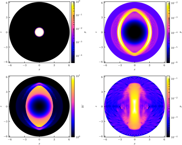
Next, we test the relativistic MHD evolution with a magnetized spherical explosion problem Cerdá-Durán et al. 2008. This test is the natural extension of the cylindrical explosion test proposed in Komissarov 1999 to spherical coordinates, setting up spherically symmetric initial data. Using the same jump conditions as Komissarov 1999, the initial data consists of an overdense ( $\rho=$1\text{\times}{10}^{-2}$$ , $p=1.0$ ) ball of radius 1.0. From a radius of 0.8 onwards, the solution is matched in an exponential decay to the surrounding medium ( $\rho=1\times 10^{-4}$ , $p=3\times 10^{-5}$ ). The initial pressure profile in the $y=0$ plane is shown in the top left panel of Fig. 2. We are using a $\Gamma-$ law equation of state (EOS) using $\Gamma=4/3$ . In the magnetized case the entire domain is initially threaded by a constant magnitude magnetic field parallel to the z-axis ( $B^{z}=0.1$ ), and the fluid velocity is set to zero everywhere in the domain initially. As in the relativistic shock reflection problem, we use fixed background Minkowski spacetime for this test problem.

We first model a magnetized spherical explosion in axisymmetry, using $(n_{r}=160,n_{\theta}=80,n_{\varphi}=4)$ points, with the outer boundary $r_{\mathrm{max}}=6.0$ . We use the HLLE Riemann solver and different reconstruction methods for this test. The final distributions at $t=4$ for the pressure $P$ and Lorentz factor $W$ in the $y=0$ plane are shown in the top right and bottom panels of Fig. 2.

In the initially overdense explosion region, the fluid is only weakly magnetized, while being strongly magnetized in the ambient medium. This results in a rich flow morphology in which the fast magnetosonic wave travels out ahead in spherical symmetry at almost the speed of light, while the Alfvén wave shows a $\cos\theta$ dependence in propagation speed, traveling close to the speed of light parallel to the initial magnetic field, while being significantly slowed down in the direction perpendicular to the magnetic field, shown in the top right panel of Fig. 2 (see the discussion in Cerdá-Durán et al. 2008).

During the explosion, the magnetic field is expelled from the initial explosion region, leaving a spherically symmetric low-density region behind in which the fluid is at rest, as evidenced by the plot of the Lorentz factor in the bottom left panel of Fig. 2. The results seem to be in very good qualitative agreement with the results presented in Cerdá-Durán et al. 2008 (spherical coordinates and axisymmetry) and Cipolletta et al. 2019 (Cartesian coordinates).

As a final axisymmetric test we perform the same explosion, but with an initial magnetic field of much larger strength $B^{z}=1.0$ . This is a very demanding test for which we have used global Lax-Friedrichs fluxes and TVD reconstruction with the Minmod limiter as they are more diffusive. In the bottom right panel of Fig. 2, we plot the pressure distribution at $t=4$ in the $y=0$ plane for this test. The morphology of the explosion changes completely and becomes bar-shaped, as seen in Cartesian simulations of magnetized cylindrical and spherical explosions (see e.g. Beckwith and Stone 2011; Cipolletta et al. 2019). Compared to the more weakly magnetized explosion, more noise can be seen in the ambient region. As discussed in Beckwith and Stone 2011, this test is most strenuous on the conservative to primitive solver, so we believe that the noise is due to inversion failures.

Next, we test the code by modeling an off-center spherical explosion, both in relativistic HD and relativistic MHD. As this test does not exploit the symmetries of our spherical coordinate system, we perform it in full 3D. The initial data are identical to the axisymmetric test described above, except the center of the explosion region has been moved to $(x=1.1,y=0,z=0)$ . The resulting initial pressure profile in the $y=0$ plane is shown in the top left panel of Fig 3. In addition, compared to the axisymmetric explosion, the initial magnetic field $B^{z}=0.1$ has been tilted by $45^{\circ}$ about the x-axis. This results in initial data that do not reflect the symmetries of the spherical coordinate system at all. For this full 3D test, we use $(n_{r}=160,n_{\theta}=80,n_{\varphi}=160)$ points, and use the azimuthal FFT filter to increase the time step to what it would have been, had the simulation been performed with $n_{\varphi}=6$ points.

We first perform two tests setting the magnetic field to zero initially, using TVD and MP5 reconstructions. The results for the two different reconstruction schemes are shown in the top right and bottom left panels of Fig. 3, respectively. When using TVD, there are no visible artifacts arising from the (in hydro only) spherically symmetric shock passing through the origin and axis. The rarefaction region is seen to be spherically symmetric as well, showing no artifacts. When using MP5, the shock width is clearly reduced compared to TVD reconstruction, demonstrating a superior capture of the shock with the higher order reconstruction, but small artifacts in those parts of the shock that have passed the origin and polar axis can be seen. A similar test in hydro is presented in Skinner et al. 2019. The bottom right panel of Fig 3 shows the final pressure distribution for the off-centered, tilted magnetic field spherical explosion, which was performed using global Lax-Friedrichs fluxes and TVD reconstruction with a Minmod limiter. This test displays more pronounced effects of the magnetized shock passing through origin and polar axis, showing primitive recovery failures at the polar axis. The global morphology is captured well nevertheless.

Figure 5: Convergence order in conservation of

D

and

\tau

for the spherical off-centered explosion with a magnetic field initially tilted by

45^{\circ}

about the x-axis. See main text for details.

It is worth noting that the numerical artifacts that can be seen in the bottom panels of Fig 3 are not concerning at all. The test setup was deliberately chosen to push the code to its limits by not exhibiting any (approximate) symmetries the framework was designed for, and is a difficult test to pass even for Cartesian codes Cipolletta et al. 2019.

Finally, in Fig. 4 we plot the final pressure distribution in the $x=1.1$ plane, i.e. the plane vertically cutting through the initial center of the explosion region. The flow morphology observed in the axisymmetric case (top right panel of Fig. 2) is clearly seen to be present and tilted by $45^{\circ}$ , which is precisely the symmetry axis picked out by the tilted magnetic field initially threading the computational domain.

As explained in Sec. II.2.4 above, the conserved rest mass density $D$ is not conserved to round off in our framework due to the appearance of geometric source terms in the evolution equation for $D$ (67). Furthermore, the FFT filter we employ to circumvent the severe CFL limit in full 3D simulations is inherently non-conservative as well. We therefore check for the convergence of the total rest mass and total energy conservation ( $s_{\tau}$ , the source term in the evolution equation for $\tau$ (76) vanishes in Minkowski spacetime so that $\tau$ should be exactly conserved as well). To do so, we calculate $\varepsilon_{A}(t)$ , the volume integrated error arising from nonconservation of a quantity $A=(D,\tau)$ at time $t$ as:

\varepsilon_{A}(t)=\int_{\Sigma}\left(A(t)-A(0)\right)\sqrt{\hat{\gamma}}\,drd\theta d\varphi,

(151)

and calculate the convergence order $q_{A}(t)$ as Bona et al. 1998:

q_{A}(t)=\frac{1}{\ln(f)}\ln\left(\frac{||\varepsilon_{A}(t)||^{\mathrm{low}}}{||\varepsilon_{A}(t)||^{\mathrm{high}}}\right),

(152)

where $f$ is the ratio between the different resolutions used in the convergence test. We calculate $q_{A}(t)$ in the most demanding variant of the spherical explosion, the off-centered explosion with a tilted initial magnetic field, using two different resolutions of $(n_{r},n_{\theta},n_{\varphi})=(112,56,112)$ and (160,80,160), corresponding to $f\approx\sqrt{2}$ and show the time evolution of $q_{A}(t)$ in Fig. 5. In our numerical scheme, we would expect the convergence order to be between 1 and 2, as our method is 2nd order accurate while reducing to first order in the presence of shocks. The convergence order of the conservation of total rest mass lies within that region, while for the total energy it drops below first order at the time the numerical artifacts at the polar axis seen in the bottom right panel of Fig. 3 start appearing. The maximum relative error in the conservation of total rest mass and total energy in the high resolution test is $0.0016$ and $0.004$ , respectively.

Next, we turn to dynamical spacetime evolutions of uniformly rotating neutron stars, testing the coupled spacetime and GRMHD evolution of the SphericalNR framework. To test the framework in this regime, we evolve two uniformly rotating polytropes, models BU2 Stergioulas et al. 2004 and D1 Baiotti et al. 2005a, adding a weak poloidal magnetic field initially. We perform tests of two important scenarios: The long-term evolution of a stable equilibrium model, as well as the gravitational collapse of a uniformly rotating polytrope to a BH. In the long-term evolution of model BU2, we initially tilt the star’s rotation axis by $90^{\circ}$ in order to test the evolution in full 3D without symmetry assumptions. In this test, the fluid rotates through the polar axis during the entire simulation, dragging the magnetic field with it through the polar axis constantly. In the second test, we perform a simulation of the gravitational collapse of model D1, testing all aspects of our framework: the correct coupled evolution of the fCCZ4 and GRMHD equations leading to dynamical BH formation and ringdown to a Kerr BH.

Table 2: Main properties of the relativistic polytrope models BU2 Stergioulas et al. 2004 and D1 Baiotti et al. 2005a: central rest mass density

\rho_{c}

, rest- and gravitational masses

M_{0}

and

M

, the dimensionless angular momentum

J/M^{2}

, the circumferential stellar radius

R

, the ratio of polar and equatorial radii of the star

r_{p}/r_{e}

, the ratio of kinetic energy and gravitational binding energy

T/|W|

, the adiabatic index

\Gamma

, the polytropic constant

K

, and the constants prescribing the initial magnetic field

A_{b}

n_{s}

and

P_{\mathrm{cut}}

(see main text for details).

	BU2	D1
$\rho_{c}$	$1.28\text{\times}{10}^{-3}$	$3.28\text{\times}{10}^{-3}$
$M_{0}$	1.58	1.83
$M$	1.47	1.67
$J/M^{2}$	$3.19\text{\times}{10}^{-1}$	$2.07\text{\times}{10}^{-1}$
$R$	10.11	7.74
$r_{p}/r_{e}$	0.9	0.95
$T/\|W\|$	$2.44\text{\times}{10}^{-2}$	$1.17\text{\times}{10}^{-2}$
$\Gamma$	2	2
$K$	100	100
$A_{b}$	2	1
$n_{s}$	0	0
$P_{\mathrm{cut}}$	$6.55\text{\times}{10}^{-6}$	$4.25\text{\times}{10}^{-6}$

The initial data are generated with the RNS code Stergioulas and Friedman 1995, which has been incorporated as a thorn named Hydro_RNSID in the Einstein Toolkit. As with all original Cartesian thorns present in the Einstein Toolkit, in order to interface with SphericalNR we need to coordinate transform the Cartesian initial data generated by the Hydro_RNSID code and then rescale the evolved fields. In order to test the FFT filter applied to both spacetime and GRMHD fields and nontrivial dynamics in full 3D, we initially tilt the rotation axis of the neutron star by $90^{\circ}$ about the $x$ -axis so that the star’s rotation axis is initially aligned with the $y$ -axis. After generating the tilted fluid and spacetime data, we add a small initial magnetic field, following the vector-potential-based prescription of Liu et al. 2008:

$\displaystyle A_{r}$	$\displaystyle=$	$\displaystyle 0,$	(153)
$\displaystyle A_{\theta}$	$\displaystyle=$	$\displaystyle 0,$	(154)
$\displaystyle A_{\varphi}$	$\displaystyle=$	$\displaystyle A_{b}(r\sin\theta)^{2}(1-\frac{\rho}{\rho_{c}})^{n_{s}}\mathrm{max}(P_{\mathrm{cut}}-P,0),$	(155)
$\displaystyle\Phi$	$\displaystyle=$	$\displaystyle 0,$	(156)

where values of $A_{b}$ , $\rho_{c}$ , $n_{s}$ and $P_{\rm cut}$ are provided in Table 2. With this setup, the tilted, uniformly rotating star will constantly drag the magnetic field through the polar axis during the evolution. While the initial data are polytropic, we evolve the star with a $\Gamma$ -law EOS. We use a third order strong stability-preserving Runge-Kutta (SSPRK3) method Shu and Osher 1988; Gottlieb and Shu 1998¹³¹³ 13 Strong stability-preserving time discretization methods have been called TVD methods historically Gottlieb et al. 2001., implemented in the MoL thorn Löffler et al. 2012, the HLLE Riemann solver and WENO-Z reconstruction for the simulations presented here. We have also tried ePPM and MP5 reconstruction, but found a large symmetry breaking at late times when using those. To check for convergence of our code, we evolve three different resolutions for 29 ms, which is more than 200 dynamical timescales of the star.

The $t=0$ and $t=25$ ms distributions of $\rho$ and $b^{2}$ in the $y=0$ plane are shown in Fig. 6. The star remains very stable and very contained, and there are no large outflows from the stellar surface into the atmosphere, demonstrating the code’s capability to deal with the stellar surface. This is a difficult test, as the numerical dissipation at the stellar surface is minimal in spherical coordinates, due to the fact that the surface and computational cell surfaces are mostly aligned (in Cartesian coordinates, this effect is seen along the coordinate axes, see e.g. Fig. 3 in Radice et al. 2014). During the evolution, the quantity $b^{2}$ develops a richer morphology than it has in the beginning, which we believe results from the fact that the initial poloidal field evolves into having poloidal and toroidal components (while the initial data are uniformly rotating, the misalignment between the star’s rotation axis and the initial magnetic field dipole axis results in the generation of a toroidal magnetic field.). In order to quantify the error arising from the FFT filter and to check for the resolution dependence in the radial and angular coordinates, we plot the following diagnostics in Fig. 7: the relative error in central density and total rest mass in the top two panels, as well as the evolution of the $L^{2}$ -norm of the Hamiltonian constraint in the bottom panel.

Figure 7: Evolution of central density

\rho_{c}

(top panel), total rest mass

M_{0}

(mid panel), and L2-norm of the Hamiltonian constraint (bottom panel) for magnetized model BU2. Three different resolutions are shown in each plot.

Figure 8: Convergence study for magnetized model BU2. Top panel: Relative error in

\rho_{c}(t)

at multiple resolutions; medium and high resolution results are multiplied by the appropriate factor assuming a convergence order of 1.5. Bottom panel: Convergence order for the total rest mass

M_{0}

, ADM mass

M_{\mathrm{ADM}}

, and L1-norm of the Hamiltonian constraint.

Figure 9: Power spectral density of

\rho_{\mathrm{max}}(t)

evolution for resolutions of

(400\times 24\times 48)

(top) and

(250\times 32\times 64)

(bottom) panel. The vertical lines indicate the fundamental

(F)

and first overtone

(H_{1})

of the fundamental quasiradial (

l=0

) mode and the fundamental

(^{2}f)

and first overtone

(^{2}p_{1})

of the fundamental quadrupolar

(l=2)

mode (see Table 5 of Dimmelmeier et al. 2006).

Additionally, in Fig. 8 we show a convergence study with three different resolutions, now increasing the resolution twice by a factor of f = 1.5 in all three coordinate directions. The top panel shows the evolution of the error in the central density evolution, where the medium and higher resolution errors have been multiplied by 1.8 and 3.375, respectively, assuming a convergence order of 1.5. Our code is formally second order, while reducing to first order in the presence of shocks. The surface of the neutron star is a discontinuity, so we would expect the order of convergence to be between 1 and 2. The bottom panel shows the convergence factor for the total rest mass $M_{0}$ (158), the ADM mass evaluated as a volume integral, and the L1-norm of the Hamiltonian. As in Sec. IV.1.2, we calculate the convergence order for $M_{0}$ and $M_{\mathrm{ADM}}$ using (152), while the convergence order of the L1-norm of the Hamiltonian is calculated as Bona et al. 1998:

q_{A}(t)=\frac{1}{\ln(f)}\ln\left(\frac{||H(t)||^{\mathrm{low}}-||H(t)||^{\mathrm{med}}}{||H(t)||^{\mathrm{med}}-||H(t)||^{\mathrm{high}}}\right).

(157)

As the initial magnetic field is small, and the tilted rotation axis of the star should not affect its dynamics during evolution, we calculate the frequencies of oscillations in $\rho_{\mathrm{max}}(t)$ as a power spectral density for the two higher resolution runs in Fig. 9. We overlay the expected frequencies of the fundamental quasiradial $(F)$ and quadrupolar ${}^{2}f$ modes and their first overtones $(H_{1}$ and ${}^{2}p_{1})$ (taken from Table 5 of Dimmelmeier et al. 2006). In both resolutions, the fundamental modes $F$ and ${}^{2}f$ are in very good agreement with Dimmelmeier et al. 2006, however the first overtones $(H_{1}$ and ${}^{2}p_{1})$ of both fundamental modes is not visible in the simulation with lower radial but higher angular resolution, while being slightly shifted in the higher radial resolution simulation.

These tests show that our code is capable of evolving equilibrium neutron stars with magnetic fields for many timescales, in a setup (constant fluid motion and magnetic field dragging through the polar axis) that was chosen to be particularly challenging for our framework.

As our last test, we present a very important test problem for numerical relativity simulations with matter: the collapse of a neutron star to a black hole (see, e.g. Shibata et al. 2000; Baiotti et al. 2005a; Baiotti et al. 2005b; Baiotti et al. 2007; Reisswig et al. 2013; Dietrich and Bernuzzi 2015). Using the Hydro_RNSID code thorn in the Einstein Toolkit again, we setup the uniformly rotating polytrope model D1 Baiotti et al. 2005a with a weak poloidal magnetic field added initially and evolve its collapse to a Kerr BH. The initial data specifications of this model are listed in Table 2. The simulation is performed in axisymmetry, and the collapse is induced by lowering the polytropic constant $K$ everywhere in the star by $2\%$ initially. The simulation is performed using $(n_{r}=10000,n_{\theta}=32,n_{\varphi}=2)$ points, with the outer boundary placed at $r_{\mathrm{out}}=500$ . We evolve the conformal factor $W=e^{-2\phi}$ Marronetti et al. 2008, use the SSPRK3 method for time integration, and the fCCZ4 damping parameters are set to $\kappa_{1}=0.06,\kappa_{2}=0,\kappa_{3}=1$ . We use WENO-Z reconstruction, the HLLE Riemann solver, and a $\Gamma-$ law EOS with $\Gamma=2$ .

The atmosphere value for $\rho$ is set to be $10^{-8}$ times the initial density maximum $(\rho_{\mathrm{min}}=$ $3.28\text{\times}{10}^{-11}$ . This simulation requires the use of the higher atmosphere threshold in highly magnetized regions (described in Sec. III above), as the collapsing fluid leaves a highly magnetized atmosphere region behind. In these regions, we reset a cell to atmosphere if $e^{6\phi}\rho W<100e^{6\phi}\rho_{\mathrm{min}}$ .

We use the AHFinderDirect thorn Thornburg 2004; Schnetter et al. 2005 to find the AH Thornburg 2007 once it has formed during collapse, and the QuasiLocalMeasures thorn Dreyer et al. 2003; Schnetter et al. 2006 to calculate the angular momentum of the AH during the evolution. The SphericalNR interface to these Cartesian diagnostic thorns in the Einstein Toolkit is described in Mewes et al. 2018. The BH spin is measured using a surface integral on the AH Dreyer et al. 2003 or the flat space rotational Killing vector method Campanelli et al. 2007; Mewes et al. 2015.

Deep inside the horizon, for points with coordinate radii $r<0.2\min(r_{\rm AH})$ , we set fluid variables to atmosphere values (the magnetic fields are evolved everywhere). Figure 10 shows the time evolution of radial profiles (along $\theta=d\theta/2$ ) for the density $\rho$ . The evolution of $\rho$ shows our modifications to the conservative to primitive solve in GRHydro: As the star collapses, $\rho$ is first capped to a maximum value, and then reset to atmosphere deep inside the AH once it has been found (AHFinderDirect reports the first finding of an AH at $t=103.8$ ).

Figure 11: Time evolution of various mass measurements during the collapse of model D1.

In Fig. 11 we plot different mass measurements for the duration of the simulation. Specifically, we monitor the total rest mass

M_{0}=\int_{\Sigma_{t}}\rho We^{6\phi}\sqrt{\hat{\gamma}}\,d^{3}x,

(158)

the Komar mass Komar 1959 evaluated as a volume integral (see e.g. Baumgarte and Shapiro 2010)

M_{\mathrm{Komar}}=\int_{\Sigma_{t}}\left(\alpha(E+S)-2\beta^{i}S_{i}\right)e^{6\phi}\sqrt{\hat{\gamma}}\,d^{3}x,

(159)

and the ADM mass Arnowitt et al. 2008 of the spacetime, evaluated as the sum from contributions inside a finite radius $r_{\mathrm{in}}$ , evaluated as a surface integral, and those outside $r_{\rm in}$ , evaluated as a volume integral Yo et al. 2002

Comparing with the expressions found in Yo et al. 2002 terms containing $\Delta\Gamma^{k}_{jk}$ are missing in the above expression, this is due to the fact that

\Delta\Gamma^{k}_{jk}=\frac{1}{\sqrt{\bar{\gamma}}}\hat{\mathcal{D}}_{j}\sqrt{\bar{\gamma}},

(161)

which, together with our choice of $\bar{\gamma}=\hat{\gamma}$ results in $\Delta\Gamma^{k}_{jk}=0$ . Finally, we compute the BH mass calculated as the Christodoulou mass Christodoulou 1970

M_{\mathrm{BH}}=\left(M^{2}_{\mathrm{irr}}+\frac{4\pi J^{2}}{A}\right)^{\frac{1}{2}},

(162)

where $M_{\mathrm{irr}}$ is the BH irreducible mass, $J$ the BH angular momentum, and $A$ the AH area.

The mass measurements agree well with their initial value of the equilibrium neutron star. As the collapse proceeds, the total rest mass $M_{0}$ is seen to drop when the density deep inside the star is capped (see Fig. 10) and then quickly drops to zero once an AH has been found, as we exclude points within the horizon from volume integrals. The same drop is observed in the calculation of $M_{\mathrm{Komar}}$ , which also exhibits a stronger deviation from its initial value earlier, due to the fact that it is only defined for stationary spacetimes, and the collapse is an inherently dynamical process. Towards the end of the simulations, the calculation of the ADM mass via a surface integral shows oscillations related to the gravitational radiation leaving the domain and being partially reflected at the outer boundary.

After collapse, the newly formed BH is expected to quickly settle down to a Kerr BH via the ringdown of the BH’s quasinormal modes (for a review see Berti et al. 2009). To see if our simulation reproduces this expected behavior, in Figs. 12 and 13 we plot the $l=2$ to 8, $m=0$ modes of the Weyl scalar $\Psi_{4}$ , split into even and odd $l$ -modes, respectively. The ringdown of all modes is clearly seen, as well beatings in the higher order modes, whose origin (the equal $m$ mode mixing of spherical and spheroidal harmonics) we have explained in Mewes et al. 2018.

Figure 12: Even

l=2

to 8,

m=0

modes of the Weyl scalar

\Psi_{4}

Figure 13: Odd

l=3

to 7,

m=0

modes of the Weyl scalar

\Psi_{4}

The simulation shows that our spherical GRMHD code is capable of capturing the relevant dynamics of the collapse of the magnetized uniformly rotating neutron star to a Kerr BH, capturing the post-collapse ringdown to Kerr with very high accuracy, with all modes dropping down to their initial background amplitudes.

We have extended our vacuum numerical relativity code in spherical coordinates within the Einstein Toolkit Mewes et al. 2018 to a framework that numerically solves the coupled fCCZ4/BSSN and GRMHD equations in spherical coordinates without symmetry assumptions using a reference-metric formalism.

Extending the existing spacetime evolution thorn SphericalBSSN to evolve the fCCZ4 system with constraint damping as well, enables future users of the framework with two distinct evolution systems for numerical relativity in spherical coordinates. The spacetime evolution thorn was written from scratch using NRPy+, while the implementation of the reference-metric formalism GRMHD equations derived in this work was built as an extension of the GRHydro thorn, again using NRPy+.

In our approach, the GRMHD equations in spherical coordinates acquire a “Cartesian” form, as all information about the underlying spherical coordinate system is encoded in source terms of the equations. This has allowed us to use many of the core Cartesian building blocks of the HRSC finite volume implementation already present in GRHydro without modifications (and will enable the straightforward inclusion of Cartesian finite volume building blocks such as more sophisticated Riemann solvers in the future). Without the reference-metric approach, these building blocks would need to be adapted to spherical coordinates. Further, instead of evolving the magnetic field directly, the framework evolves the cell-centered vector potential in the generalized Lorenz gauge, guaranteeing the absence of magnetic monopoles to roundoff error during the evolution by calculating the magnetic field as the curl of the vector potential.

We have tested our framework performing a set of demanding tests in flat background as well as fully dynamical spacetimes. We have chosen setups where the symmetries of the fluid are not aligned with the symmetries of the coordinate system (counter to our original motivation for developing the code). These tests include off-centered magnetized spherical explosions testing the passage of shocks and rarefaction waves through the coordinate origin and polar axis, as well as dynamical-spacetime simulations of a uniformly rotating neutron star with its rotation axis misaligned with the polar axis of the computational grid. Finally, we have shown that the code is able to perform simulations of the collapse of a magnetized uniformly rotating neutron star to a Kerr BH.

The SphericalNR framework will be made public and proposed to be included in a future official release of the Einstein Toolkit.

The authors would like to thank the anonymous referee for useful comments and suggestions. We furthermore would like to thank Eirik Endeve for a careful reading of the paper, as well as Miguel Á. Aloy, Mark J. Avara, Dennis B. Bowen, Pablo Cerdá-Durán, Isabel Cordero-Carrión, José A. Font, Roland Haas, David Hilditch, José M. Ibáñez, Kenta Kiuchi, Oleg Korobkin, Jens Mahlmann, Jonah M. Miller, Martin Obergaulinger, Scott C. Noble, David Radice, Ian Ruchlin, Erik Schnetter, and Masaru Shibata for useful discussions. We gratefully acknowledge the National Science Foundation (NSF) for financial support from Grant Nos. OAC-1550436, AST-1516150, PHY-1607520, PHY-1305730, PHY-1707946, and PHY-1726215 to Rochester Institute of Technology (RIT); PHY-1707526 to Bowdoin College; as well as OIA-1458952 and PHY-1806596 to West Virginia University. This work was also supported by NASA awards ISFM-80NSSC18K0538 and TCAN-80NSSC18K1488, as well as through sabbatical support from the Simons Foundation (Grant No. 561147 to TWB). V.M. was partially supported by the Exascale Computing Project (17-SC-20-SC), a collaborative effort of the U.S. Department of Energy (DOE) Office of Science and the National Nuclear Security Administration. Work at Oak Ridge National Laboratory is supported under contract DE-AC05-00OR22725 with the U.S. Department of Energy. V.M. also acknowledges partial support from the Spanish Ministry of Economy and Competitiveness (MINECO) through Grant No. AYA2015-66899-C2-1-P, and RIT for the FGWA SIRA initiative. This work used the Extreme Science and Engineering Discovery Environment (XSEDE) [allocation TG-PHY060027N], which is supported by NSF grant No. ACI-1548562, and the BlueSky and Green Prairies Clusters at RIT, which are supported by NSF grants AST-1028087, PHY-0722703, PHY-1229173, and PHY-1726215. Funding for computer equipment to support the development of SENR/NRPy+ was provided in part by NSF EPSCoR Grant OIA-1458952 to West Virginia University. Computational resources were also provided by the Blue Waters sustained-petascale computing NSF project OAC-1516125. All figures in this paper were created using Matplotlib Hunter 2007 for which we have used the scidata sci library to import Carpet data.

$\displaystyle M_{\mathrm{ADM}}$

$\displaystyle=\frac{1}{16\pi}\oint_{r_{\mathrm{in}}}$

$\displaystyle(\Delta\Gamma^{r}-8e^{\phi}\bar{\mathcal{D}}^{r}\phi)\,\sqrt{\hat{\gamma}}\,d\theta d\varphi$

$\displaystyle+\frac{1}{16\pi}\int_{r>r_{\mathrm{in}}}\Big[$

$\displaystyle e^{5\phi}(16\pi E+\bar{A}_{ij}\bar{A}^{ij}-\frac{2}{3}K^{2})$

$\displaystyle-\Delta\Gamma^{ijk}\Delta\Gamma_{jik}$

$\displaystyle+(1-e^{\phi})\bar{R}\Big]\,\sqrt{\hat{\gamma}}\,drd\theta d\varphi.$

Abbott et al. (2016a) B. P. Abbott et al. (LIGO Scientific, Virgo), Phys. Rev. Lett. 116, 061102 (2016a), arXiv:1602.03837 [gr-qc] .
Abbott et al. (2016b) B. P. Abbott et al. (LIGO Scientific, Virgo), Phys. Rev. Lett. 116, 241102 (2016b), arXiv:1602.03840 [gr-qc] .
Abbott et al. (2016c) B. P. Abbott et al. (LIGO Scientific, Virgo), Phys. Rev. Lett. 116, 241103 (2016c), arXiv:1606.04855 [gr-qc] .
Abbott et al. (2017a) B. P. Abbott et al. (LIGO Scientific, VIRGO), Phys. Rev. Lett. 118, 221101 (2017a), [Erratum: Phys. Rev. Lett.121,no.12,129901(2018)], arXiv:1706.01812 [gr-qc] .
Abbott et al. (2017b) B. P. Abbott et al. (LIGO Scientific, Virgo), Astrophys. J. 851, L35 (2017b), arXiv:1711.05578 [astro-ph.HE] .
Abbott et al. (2017c) B. P. Abbott et al. (LIGO Scientific, Virgo), Phys. Rev. Lett. 119, 141101 (2017c), arXiv:1709.09660 [gr-qc] .
Abbott et al. (2017d) B. P. Abbott et al. (LIGO Scientific, Virgo), Phys. Rev. Lett. 119, 161101 (2017d), arXiv:1710.05832 [gr-qc] .
Abbott et al. (2017e) B. P. Abbott et al. (LIGO Scientific, Virgo, Fermi GBM, INTEGRAL, IceCube, AstroSat Cadmium Zinc Telluride Imager Team, IPN, Insight-Hxmt, ANTARES, Swift, AGILE Team, 1M2H Team, Dark Energy Camera GW-EM, DES, DLT40, GRAWITA, Fermi-LAT, ATCA, ASKAP, Las Cumbres Observatory Group, OzGrav, DWF (Deeper Wider Faster Program), AST3, CAASTRO, VINROUGE, MASTER, J-GEM, GROWTH, JAGWAR, CaltechNRAO, TTU-NRAO, NuSTAR, Pan-STARRS, MAXI Team, TZAC Consortium, KU, Nordic Optical Telescope, ePESSTO, GROND, Texas Tech University, SALT Group, TOROS, BOOTES, MWA, CALET, IKI-GW Follow-up, H.E.S.S., LOFAR, LWA, HAWC, Pierre Auger, ALMA, Euro VLBI Team, Pi of Sky, Chandra Team at McGill University, DFN, ATLAS Telescopes, High Time Resolution Universe Survey, RIMAS, RATIR, SKA South Africa/MeerKAT), Astrophys. J. 848, L12 (2017e), arXiv:1710.05833 [astro-ph.HE] .
Abbott et al. (2017f) B. P. Abbott et al. (LIGO Scientific, Virgo, Fermi-GBM, INTEGRAL), Astrophys. J. 848, L13 (2017f), arXiv:1710.05834 [astro-ph.HE] .
Aasi et al. (2014) J. Aasi, B. P. Abbott, R. Abbott, T. Abbott, M. R. Abernathy, T. Accadia, F. Acernese, K. Ackley, C. Adams, T. Adams, and et al., Classical and Quantum Gravity 31, 115004 (2014), arXiv:1401.0939 [gr-qc] .
Metzger (2017) B. D. Metzger, Living Reviews in Relativity 20, 3 (2017), arXiv:1610.09381 [astro-ph.HE] .
Rosswog (2015) S. Rosswog, International Journal of Modern Physics D 24, 1530012-52 (2015), arXiv:1501.02081 [astro-ph.HE] .
Shibata and Uryū (2000) M. Shibata and K. ō. Uryū, Phys. Rev. D 61, 064001 (2000), arXiv:gr-qc/9911058 [gr-qc] .
Pretorius (2005) F. Pretorius, Physical Review Letters 95, 121101 (2005), arXiv:gr-qc/0507014 [gr-qc] .
Campanelli et al. (2006) M. Campanelli, C. O. Lousto, P. Marronetti, and Y. Zlochower, Physical Review Letters 96, 111101 (2006), arXiv:gr-qc/0511048 [gr-qc] .
Baker et al. (2006) J. G. Baker, J. Centrella, D.-I. Choi, M. Koppitz, and J. van Meter, Physical Review Letters 96, 111102 (2006), arXiv:gr-qc/0511103 [gr-qc] .
Shibata and Uryū (2006) M. Shibata and K. Uryū, Phys. Rev. D 74, 121503 (2006), arXiv:gr-qc/0612142 [gr-qc] .
Anderson et al. (2008) M. Anderson, E. W. Hirschmann, L. Lehner, S. L. Liebling, P. M. Motl, D. Neilsen, C. Palenzuela, and J. E. Tohline, Physical Review Letters 100, 191101 (2008), arXiv:0801.4387 [gr-qc] .
Liu et al. (2008) Y. T. Liu, S. L. Shapiro, Z. B. Etienne, and K. Taniguchi, Phys. Rev. D 78, 024012 (2008), arXiv:0803.4193 .
Chawla et al. (2010) S. Chawla, M. Anderson, M. Besselman, L. Lehner, S. L. Liebling, P. M. Motl, and D. Neilsen, Phys. Rev. Lett. 105, 111101 (2010), arXiv:1006.2839 [gr-qc] .
Shibata and Sekiguchi (2005) M. Shibata and Y.-I. Sekiguchi, Phys. Rev. D 72, 044014 (2005), astro-ph/0507383 .
Duez et al. (2005) M. D. Duez, Y. T. Liu, S. L. Shapiro, and B. C. Stephens, Phys. Rev. D 72, 024028 (2005), astro-ph/0503420 .
Antón et al. (2006) L. Antón, O. Zanotti, J. A. Miralles, J. M. Martí, J. M. Ibáñez, J. A. Font, and J. A. Pons, Astrophys. J. 637, 296 (2006), astro-ph/0506063 .
Anderson et al. (2006) M. Anderson, E. W. Hirschmann, S. L. Liebling, and D. Neilsen, Classical and Quantum Gravity 23, 6503 (2006), gr-qc/0605102 .
Giacomazzo and Rezzolla (2007) B. Giacomazzo and L. Rezzolla, Classical and Quantum Gravity 24, S235 (2007), gr-qc/0701109 .
Cerdá-Durán et al. (2008) P. Cerdá-Durán, J. A. Font, L. Antón, and E. Müller, Astron. Astrophys. 492, 937 (2008), arXiv:0804.4572 .
Bucciantini and Del Zanna (2011) N. Bucciantini and L. Del Zanna, Astron. Astrophys. 528, A101 (2011), arXiv:1010.3532 [astro-ph.IM] .
Mösta et al. (2014) P. Mösta, B. C. Mundim, J. A. Faber, R. Haas, S. C. Noble, T. Bode, F. Löffler, C. D. Ott, C. Reisswig, and E. Schnetter, Classical and Quantum Gravity 31, 015005 (2014), arXiv:1304.5544 [gr-qc] .
Etienne et al. (2015) Z. B. Etienne, V. Paschalidis, R. Haas, P. Mösta, and S. L. Shapiro, Classical and Quantum Gravity 32, 175009 (2015), arXiv:1501.07276 [astro-ph.HE] .
Dionysopoulou et al. (2013) K. Dionysopoulou, D. Alic, C. Palenzuela, L. Rezzolla, and B. Giacomazzo, Phys. Rev. D 88, 044020 (2013), arXiv:1208.3487 [gr-qc] .
Kidder et al. (2017) L. E. Kidder, S. E. Field, F. Foucart, E. Schnetter, S. A. Teukolsky, A. Bohn, N. Deppe, P. Diener, F. Hébert, J. Lippuner, J. Miller, C. D. Ott, M. A. Scheel, and T. Vincent, Journal of Computational Physics 335, 84 (2017), arXiv:1609.00098 [astro-ph.HE] .
Hossein Nouri et al. (2018) F. Hossein Nouri, M. D. Duez, F. Foucart, M. B. Deaton, R. Haas, M. Haddadi, L. E. Kidder, C. D. Ott, H. P. Pfeiffer, M. A. Scheel, and B. Szilagyi, Phys. Rev. D 97, 083014 (2018), arXiv:1710.07423 [astro-ph.HE] .
Fambri et al. (2018) F. Fambri, M. Dumbser, S. Köppel, L. Rezzolla, and O. Zanotti, Mon. Not. R. Astron. Soc. 477, 4543 (2018), arXiv:1801.02839 [physics.comp-ph] .
Cipolletta et al. (2019) F. Cipolletta, J. V. Kalinani, B. Giacomazzo, and R. Ciolfi, (2019), arXiv:1912.04794 [astro-ph.HE] .
Koide et al. (1999) S. Koide, K. Shibata, and T. Kudoh, Astrophys. J. 522, 727 (1999).
De Villiers and Hawley (2003) J.-P. De Villiers and J. F. Hawley, Astrophys. J. 589, 458 (2003), astro-ph/0210518 .
Gammie et al. (2003) C. F. Gammie, J. C. McKinney, and G. Tóth, Astrophys. J. 589, 444 (2003), astro-ph/0301509 .
Anninos et al. (2005) P. Anninos, P. C. Fragile, and J. D. Salmonson, Astrophys. J. 635, 723 (2005), astro-ph/0509254 .
Komissarov (2004) S. S. Komissarov, Mon. Not. R. Astron. Soc. 350, 1431 (2004), astro-ph/0402430 .
Noble et al. (2006) S. C. Noble, C. F. Gammie, J. C. McKinney, and L. Del Zanna, Astrophys. J. 641, 626 (2006), astro-ph/0512420 .
Bonazzola et al. (2007) S. Bonazzola, L. Villain, and M. Bejger, Classical and Quantum Gravity 24, S221 (2007), gr-qc/0612049 .
Noble et al. (2009) S. C. Noble, J. H. Krolik, and J. F. Hawley, Astrophys. J. 692, 411 (2009), arXiv:0808.3140 .
White et al. (2016) C. J. White, J. M. Stone, and C. F. Gammie, Astrophys. J. Supplement Series 225, 22 (2016), arXiv:1511.00943 [astro-ph.HE] .
Porth et al. (2017) O. Porth, H. Olivares, Y. Mizuno, Z. Younsi, L. Rezzolla, M. Moscibrodzka, H. Falcke, and M. Kramer, Computational Astrophysics and Cosmology 4, 1 (2017), arXiv:1611.09720 [gr-qc] .
Liska et al. (2019) M. Liska, K. Chatterjee, A. e. Tchekhovskoy, D. Yoon, D. van Eijnatten, C. Hesp, S. Markoff, A. Ingram, and M. van der Klis, arXiv e-prints , arXiv:1912.10192 (2019), arXiv:1912.10192 [astro-ph.HE] .
Cerdá-Durán et al. (2005) P. Cerdá-Durán, G. Faye, H. Dimmelmeier, J. A. Font, J. M. Ibáñez, E. Müller, and G. Schäfer, Astron. Astrophys. 439, 1033 (2005), astro-ph/0412611 .
Cordero-Carrión et al. (2009) I. Cordero-Carrión, P. Cerdá-Durán, H. Dimmelmeier, J. L. Jaramillo, J. Novak, and E. Gourgoulhon, Phys. Rev. D 79, 024017 (2009), arXiv:0809.2325 [gr-qc] .
Cordero-Carrión et al. (2012) I. Cordero-Carrión, P. Cerdá-Durán, and J. M. Ibáñez, Phys. Rev. D 85, 044023 (2012), arXiv:1108.0571 [gr-qc] .
Wilson et al. (1996) J. R. Wilson, G. J. Mathews, and P. Marronetti, Phys. Rev. D 54, 1317 (1996), gr-qc/9601017 .
Isenberg (2008) J. A. Isenberg, International Journal of Modern Physics D 17, 265 (2008), gr-qc/0702113 .
Janka et al. (2007) H. T. Janka, K. Langanke, A. Marek, G. Martínez-Pinedo, and B. Müller, Physics Reports 442, 38 (2007), arXiv:astro-ph/0612072 [astro-ph] .
Burrows (2013) A. Burrows, Reviews of Modern Physics 85, 245 (2013), arXiv:1210.4921 [astro-ph.SR] .
Shibata and Taniguchi (2011) M. Shibata and K. Taniguchi, Living Reviews in Relativity 14, 6 (2011).
Faber and Rasio (2012) J. A. Faber and F. A. Rasio, Living Reviews in Relativity 15, 8 (2012), arXiv:1204.3858 [gr-qc] .
Baiotti and Rezzolla (2017) L. Baiotti and L. Rezzolla, Reports on Progress in Physics 80, 096901 (2017), arXiv:1607.03540 [gr-qc] .
Duez and Zlochower (2019) M. D. Duez and Y. Zlochower, Reports on Progress in Physics 82, 016902 (2019), arXiv:1808.06011 [gr-qc] .
Radice et al. (2020) D. Radice, S. Bernuzzi, and A. Perego, (2020), 10.1146/annurev-nucl-013120-114541, arXiv:2002.03863 [astro-ph.HE] .
Lorimer (2005) D. R. Lorimer, Living Reviews in Relativity 8, 7 (2005), arXiv:astro-ph/0511258 [astro-ph] .
Turolla et al. (2015) R. Turolla, S. Zane, and A. L. Watts, Reports on Progress in Physics 78, 116901 (2015), arXiv:1507.02924 [astro-ph.HE] .
Mereghetti et al. (2015) S. Mereghetti, J. Pons, and A. Melatos, Space Sci. Rev. 191, 315 (2015), arXiv:1503.06313 [astro-ph.HE] .
Kaspi and Beloborodov (2017) V. M. Kaspi and A. M. Beloborodov, Annual Review of Astronomy and Astrophysics 55, 261 (2017), arXiv:1703.00068 [astro-ph.HE] .
Abramowicz and Fragile (2013) M. A. Abramowicz and P. C. Fragile, Living Reviews in Relativity 16, 1 (2013), arXiv:1104.5499 [astro-ph.HE] .
Call et al. (2010) J. M. Call, J. E. Tohline, and L. Lehner, Classical and Quantum Gravity 27, 175002 (2010).
Mignone et al. (2012) A. Mignone, M. Flock, M. Stute, S. M. Kolb, and G. Muscianisi, Astron. Astrophys. 545, A152 (2012), arXiv:1207.2955 [astro-ph.IM] .
Byerly et al. (2014) Z. D. Byerly, B. Adelstein-Lelbach, J. E. Tohline, and D. C. Marcello, Astrophys. J. Supplement Series 212, 23 (2014), arXiv:1404.5942 [astro-ph.SR] .
Shibata and Nakamura (1995) M. Shibata and T. Nakamura, Phys. Rev. D 52, 5428 (1995).
Baumgarte and Shapiro (1999) T. W. Baumgarte and S. L. Shapiro, Phys. Rev. D 59, 024007 (1999), arXiv:gr-qc/9810065 [gr-qc] .
Bonazzola et al. (2004) S. Bonazzola, E. Gourgoulhon, P. Grandclément, and J. Novak, Phys. Rev. D 70, 104007 (2004), arXiv:gr-qc/0307082 [gr-qc] .
Shibata et al. (2004) M. Shibata, K. Uryū, and J. L. Friedman, Phys. Rev. D 70, 044044 (2004), arXiv:gr-qc/0407036 [gr-qc] .
Gourgoulhon (2007) E. Gourgoulhon, arXiv e-prints (2007), arXiv:gr-qc/0703035 [gr-qc] .
Brown (2009) J. D. Brown, Phys. Rev. D 79, 104029 (2009), arXiv:0902.3652 [gr-qc] .
Montero and Cordero-Carrión (2012) P. J. Montero and I. Cordero-Carrión, Phys. Rev. D 85, 124037 (2012), arXiv:1204.5377 [gr-qc] .
Baumgarte et al. (2013) T. W. Baumgarte, P. J. Montero, I. Cordero-Carrión, and E. Müller, Phys. Rev. D 87, 044026 (2013), arXiv:1211.6632 [gr-qc] .
Montero et al. (2014) P. J. Montero, T. W. Baumgarte, and E. Müller, Phys. Rev. D 89, 084043 (2014), arXiv:1309.7808 [gr-qc] .
Baumgarte et al. (2015) T. W. Baumgarte, P. J. Montero, and E. Müller, Phys. Rev. D 91, 064035 (2015), arXiv:1501.05259 [gr-qc] .
Sanchis-Gual et al. (2014) N. Sanchis-Gual, P. J. Montero, J. A. Font, E. Müller, and T. W. Baumgarte, Phys. Rev. D 89, 104033 (2014), arXiv:1403.3653 [gr-qc] .
Bona et al. (2003) C. Bona, T. Ledvinka, C. Palenzuela, and M. Žáček, Phys. Rev. D 67, 104005 (2003), gr-qc/0302083 .
Bernuzzi and Hilditch (2010) S. Bernuzzi and D. Hilditch, Phys. Rev. D 81, 084003 (2010), arXiv:0912.2920 [gr-qc] .
Alic et al. (2012) D. Alic, C. Bona-Casas, C. Bona, L. Rezzolla, and C. Palenzuela, Phys. Rev. D 85, 064040 (2012), arXiv:1106.2254 [gr-qc] .
Ruchlin et al. (2018) I. Ruchlin, Z. B. Etienne, and T. W. Baumgarte, Phys. Rev. D 97, 064036 (2018), arXiv:1712.07658 [gr-qc] .
Mewes et al. (2018) V. Mewes, Y. Zlochower, M. Campanelli, I. Ruchlin, Z. B. Etienne, and T. W. Baumgarte, Phys. Rev. D97, 084059 (2018), arXiv:1802.09625 [gr-qc] .
The Einstein Toolkit developers (2019) The Einstein Toolkit developers, “The Einstein Toolkit,” (2019), to find out more, visit http://einsteintoolkit.org.
Nakamura et al. (1987) T. Nakamura, K. Oohara, and Y. Kojima, Progress of Theoretical Physics Supplement 90, 1 (1987).
Alic et al. (2013) D. Alic, W. Kastaun, and L. Rezzolla, Phys. Rev. D 88, 064049 (2013), arXiv:1307.7391 [gr-qc] .
Bona and Palenzuela (2004) C. Bona and C. Palenzuela, Phys. Rev. D 69, 104003 (2004), gr-qc/0401019 .
Gundlach et al. (2005) C. Gundlach, J. M. Martin-Garcia, G. Calabrese, and I. Hinder, Class. Quant. Grav. 22, 3767 (2005), arXiv:gr-qc/0504114 [gr-qc] .
Darmois (1927) G. Darmois, Mémorial des sciences mathématiques 25, 1 (1927).
Rosen (1963) N. Rosen, Annals of Physics 22, 1 (1963).
Cornish (1964) F. H. J. Cornish, Proceedings of the Royal Society of London Series A 282, 358 (1964).
Rosen (1973) N. Rosen, General Relativity and Gravitation 4, 435 (1973).
Nahmad-Achar and Schutz (1987) E. Nahmad-Achar and B. F. Schutz, General Relativity and Gravitation 19, 655 (1987).
Katz (1985) J. Katz, Classical and Quantum Gravity 2, 423 (1985).
Katz et al. (1988) J. Katz, D. Lynden-Bell, and W. Israel, Classical and Quantum Gravity 5, 971 (1988).
Katz and Ori (1990) J. Katz and A. Ori, Classical and Quantum Gravity 7, 787 (1990).
Gourgoulhon and Bonazzola (1994) E. Gourgoulhon and S. Bonazzola, Classical and Quantum Gravity 11, 443 (1994).
Cook and Baumgarte (2008) G. B. Cook and T. W. Baumgarte, Phys. Rev. D 78, 104016 (2008), arXiv:0810.4493 [gr-qc] .
Marronetti et al. (2008) P. Marronetti, W. Tichy, B. Brügmann, J. González, and U. Sperhake, Phys. Rev. D 77, 064010 (2008), arXiv:0709.2160 [gr-qc] .
Bona et al. (1995) C. Bona, J. Massó, E. Seidel, and J. Stela, Physical Review Letters 75, 600 (1995), arXiv:gr-qc/9412071 [gr-qc] .
Alcubierre et al. (2003) M. Alcubierre, B. Brügmann, P. Diener, M. Koppitz, D. Pollney, E. Seidel, and R. Takahashi, Phys. Rev. D 67, 084023 (2003), arXiv:gr-qc/0206072 [gr-qc] .
Lightman et al. (1975) A. P. Lightman, W. H. Press, R. H. Price, and S. A. Teukolsky, Problem Book in Relativity and Gravitation (Princeton University Press, 1975).
Banyuls et al. (1997) F. Banyuls, J. A. Font, J. M. Ibáñez, J. M. Martí, and J. A. Miralles, Astrophys. J. 476, 221 (1997).
Dimmelmeier (2001) H. Dimmelmeier, General relativistic collapse of rotating stellar cores in axisymmetry, Ph.D. thesis, Technische Universität München (2001).
Baumgarte and Shapiro (2010) T. W. Baumgarte and S. L. Shapiro, Numerical Relativity: Solving Einstein’s Equations on the Computer (Cambridge University Press, 2010).
Rezzolla and Zanotti (2013) L. Rezzolla and O. Zanotti, Relativistic hydrodynamics (Oxford University Press, 2013).
Cerdá-Durán and Font (2007) P. Cerdá-Durán and J. A. Font, Classical and Quantum Gravity 24, S155 (2007), arXiv:astro-ph/0703593 [astro-ph] .
Brackbill and Barnes (1980) J. U. Brackbill and D. C. Barnes, Journal of Computational Physics 35, 426 (1980).
Tóth (2000) G. Tóth, Journal of Computational Physics 161, 605 (2000).
Dedner et al. (2002) A. Dedner, F. Kemm, D. Kröner, C.-D. Munz, T. Schnitzer, and M. Wesenberg, Journal of Computational Physics 175, 645 (2002).
Evans and Hawley (1988) C. R. Evans and J. F. Hawley, Astrophys. J. 332, 659 (1988).
Obergaulinger (2008) M. Obergaulinger, Astrophysical magnetohydrodynamics and radiative transfer: numerical methods and applications, Ph.D. thesis, Max-Planck-Institut für Astrophysik, Garching bei München (2008).
Hilditch and Schoepe (2019) D. Hilditch and A. Schoepe, Phys. Rev. D 99, 104034 (2019).
Baumgarte and Shapiro (2003) T. W. Baumgarte and S. L. Shapiro, Astrophys. J. 585, 921 (2003), arXiv:astro-ph/0211340 [astro-ph] .
Farris et al. (2012) B. D. Farris, R. Gold, V. Paschalidis, Z. B. Etienne, and S. L. Shapiro, Phys. Rev. Lett. 109, 221102 (2012), arXiv:1207.3354 [astro-ph.HE] .
Schnetter (2010) E. Schnetter, Classical and Quantum Gravity 27, 167001 (2010), arXiv:1003.0859 [gr-qc] .
Greenberg and Leroux (1996) J. M. Greenberg and A. Y. Leroux, SIAM Journal on Numerical Analysis 33, 1 (1996).
Papadopoulos and Font (1999) P. Papadopoulos and J. A. Font, (1999), gr-qc/9912054 .
Neilsen and Choptuik (2000) D. W. Neilsen and M. W. Choptuik, Classical and Quantum Gravity 17, 733 (2000), gr-qc/9904052 .
McKinney et al. (2012) J. C. McKinney, A. Tchekhovskoy, and R. D. Blandford, Mon. Not. R. Astron. Soc. 423, 3083 (2012), arXiv:1201.4163 [astro-ph.HE] .
Lax and Wendroff (1960) P. Lax and B. Wendroff, Commun. Pure Appl. Math. 13, 217 (1960).
LeVeque (1992) R. J. LeVeque, Numerical methods for conservation laws, Vol. 132 (Springer, 1992).
Font (2008) J. A. Font, Living Reviews in Relativity 11 (2008), 10.12942/lrr-2008-7.
Godunov (1959) S. K. Godunov, Mat. Sb. 89, 271 (1959).
Toro (2013) E. F. Toro, Riemann solvers and numerical methods for fluid dynamics: a practical introduction (Springer Science & Business Media, 2013).
Shu and Osher (1988) C.-W. Shu and S. Osher, Journal of Computational Physics 77, 439 (1988).
Mönchmeyer and Müller (1989) R. Mönchmeyer and E. Müller, Astron. Astrophys. 217, 351 (1989).
Mignone (2014) A. Mignone, Journal of Computational Physics 270, 784 (2014), arXiv:1404.0537 [physics.comp-ph] .
Baiotti et al. (2005a) L. Baiotti, I. Hawke, P. J. Montero, F. Löffler, L. Rezzolla, N. Stergioulas, J. A. Font, and E. Seidel, Phys. Rev. D 71, 024035 (2005a), arXiv:gr-qc/0403029 [gr-qc] .
Hawke et al. (2005) I. Hawke, F. Löffler, and A. Nerozzi, Phys. Rev. D 71, 104006 (2005), arXiv:gr-qc/0501054 [gr-qc] .
Löffler et al. (2012) F. Löffler, J. Faber, E. Bentivegna, T. Bode, P. Diener, R. Haas, I. Hinder, B. C. Mundim, C. D. Ott, E. Schnetter, G. Allen, M. Campanelli, and P. Laguna, Classical and Quantum Gravity 29, 115001 (2012), arXiv:1111.3344 [gr-qc] .
(130) “Cactus Computational Toolkit,” http://www.cactuscode.org.
(131) “Carpet: Adaptive mesh refinement for the Cactus framework,” https://bitbucket.org/eschnett/carpet/src/master/.
Goodale et al. (2003) T. Goodale, G. Allen, G. Lanfermann, J. Massó, T. Radke, E. Seidel, and J. Shalf, in Proceedings of the 5th International Conference on High Performance Computing for Computational Science, edited by J. M. L. M. Palma, A. A. Sousa, J. Dongarra, and V. Hernández (Springer Berlin Heidelberg, Berlin, Heidelberg, 2003) Chap. The Cactus Framework and Toolkit: Design and Applications, pp. 197–227.
Schnetter et al. (2004) E. Schnetter, S. H. Hawley, and I. Hawke, Classical and Quantum Gravity 21, 1465 (2004), arXiv:gr-qc/0310042 [gr-qc] .
Ruchlin et al. (2018) I. Ruchlin, Z. B. Etienne, and T. W. Baumgarte, Phys. Rev. D97, 064036 (2018), arXiv:1712.07658 [gr-qc] .
Etienne (2020) Z. B. Etienne, “NRPy+ web page,” (2020), http://nrpyplus.net.
Roe (1986) P. L. Roe, Annual Review of Fluid Mechanics 18, 337 (1986).
van Leer (1977) B. van Leer, Journal of Computational Physics 23, 276 (1977).
Colella and Woodward (1984) P. Colella and P. R. Woodward, Journal of Computational Physics 54, 174 (1984).
McCorquodale and Colella (2011) P. McCorquodale and P. Colella, Communications in Applied Mathematics and Computational Science 6, 1 (2011).
Reisswig et al. (2013) C. Reisswig, R. Haas, C. D. Ott, E. Abdikamalov, P. Mösta, D. Pollney, and E. Schnetter, Phys. Rev. D 87, 064023 (2013), arXiv:1212.1191 [astro-ph.HE] .
Suresh and Huynh (1997) A. Suresh and H. T. Huynh, Journal of Computational Physics 136, 83 (1997).
Harten et al. (1997) A. Harten, B. Engquist, S. Osher, and S. R. Chakravarthy, Journal of Computational Physics 131, 3 (1997).
Shu (1998) C.-W. Shu, in Advanced numerical approximation of nonlinear hyperbolic equations (Springer, 1998) pp. 325–432.
Castro et al. (2011) M. Castro, B. Costa, and W. S. Don, Journal of Computational Physics 230, 1766 (2011).
Einfeldt (1988) B. Einfeldt, SIAM Journal on Numerical Analysis 25, 294 (1988).
Harten (1983) A. Harten, Journal of Computational Physics 49, 357 (1983).
Giacomazzo et al. (2011) B. Giacomazzo, L. Rezzolla, and L. Baiotti, Phys. Rev. D 83, 044014 (2011), arXiv:1009.2468 [gr-qc] .
Mocz (2017) P. Mocz, Journal of Computational Physics 328, 221 (2017).
Kreiss and Oliger (1973) H.-O. Kreiss and J. Oliger, Methods for the approximate solution of time dependent problems, 10 (International Council of Scientific Unions, World Meteorological Organization, 1973).
Etienne et al. (2010) Z. B. Etienne, Y. T. Liu, and S. L. Shapiro, Phys. Rev. D 82, 084031 (2010), arXiv:1007.2848 [astro-ph.HE] .
Wu and Shu (2019) K. Wu and C.-W. Shu, Numer. Math. 142, 995–1047 (2019), arXiv:1807.11467 [math.NA] .
Shibata et al. (2007) M. Shibata, Y.-I. Sekiguchi, and R. Takahashi, Progress of Theoretical Physics 118, 257 (2007), arXiv:0709.1766 [astro-ph] .
Siegel et al. (2018) D. M. Siegel, P. Mösta, D. Desai, and S. Wu, Astrophys. J. 859, 71 (2018), arXiv:1712.07538 [astro-ph.HE] .
Wu (2017) K. Wu, Phys. Rev. D 95, 103001 (2017), arXiv:1610.06274 [math.NA] .
Wu and Tang (2018) K. Wu and H. Tang, Zeitschrift Angewandte Mathematik und Physik 69, 84 (2018), arXiv:1709.05838 [math.NA] .
Boyd (2001) J. P. Boyd, Boyd, J.P. 2001, Chebyshev and Fourier Spectral Methods, 2nd edn., Dover books on mathematics (Mineola, NY: Dover Publications), ISBN 0486411834. (2001) p. 2001.
Ronchi et al. (1996) C. Ronchi, R. Iacono, and P. Paolucci, Journal of Computational Physics 124, 93 (1996).
Gómez et al. (1997) R. Gómez, L. Lehner, P. Papadopoulos, and J. Winicour, Classical and Quantum Gravity 14, 977 (1997), arXiv:gr-qc/9702002 [gr-qc] .
Bishop et al. (1997) N. T. Bishop, R. Gómez, L. Lehner, M. Maharaj, and J. Winicour, Phys. Rev. D 56, 6298 (1997), arXiv:gr-qc/9708065 [gr-qc] .
Kageyama and Sato (2004) A. Kageyama and T. Sato, Geochemistry, Geophysics, Geosystems 5, Q09005 (2004), physics/0403123 .
Zink et al. (2008) B. Zink, E. Schnetter, and M. Tiglio, Phys. Rev. D 77, 103015 (2008), arXiv:0712.0353 .
Fragile et al. (2009) P. C. Fragile, C. C. Lindner, P. Anninos, and J. D. Salmonson, Astrophys. J. 691, 482 (2009), arXiv:0809.3819 .
Wongwathanarat et al. (2010) A. Wongwathanarat, N. J. Hammer, and E. Müller, Astron. Astrophys. 514, A48 (2010), arXiv:1003.1633 [astro-ph.IM] .
Melson et al. (2015) T. Melson, H.-T. Janka, and A. Marek, Astrophys. J. Letters 801, L24 (2015), arXiv:1501.01961 [astro-ph.SR] .
Shiokawa et al. (2018) H. Shiokawa, R. M. Cheng, S. C. Noble, and J. H. Krolik, Astrophys. J. 861, 15 (2018), arXiv:1701.05610 [astro-ph.IM] .
Bowen et al. (2020) D. B. Bowen, M. Avara, V. Mewes, Y. Zlochower, S. C. Noble, M. Campanelli, H. Shiokawa, R. M. Cheng, and J. H. Krolik, arXiv e-prints , arXiv:2002.00088 (2020), arXiv:2002.00088 [physics.comp-ph] .
M. Avara, D. B. Bowen, S. C. Noble, T. Ryu, M. Campanelli, J. H. Krolik, V. Mewes, H. Shiokawa, R. Cheng (2020) M. Avara, D. B. Bowen, S. C. Noble, T. Ryu, M. Campanelli, J. H. Krolik, V. Mewes, H. Shiokawa, R. Cheng, (2020), in preparation.
Liska et al. (2018) M. Liska, C. Hesp, A. Tchekhovskoy, A. Ingram, M. van der Klis, and S. Markoff, MNRAS: Letters 474, L81 (2018), arXiv:1707.06619 [astro-ph.HE] .
Skinner et al. (2019) M. A. Skinner, J. C. Dolence, A. Burrows, D. Radice, and D. Vartanyan, Astrophys. J. Supplement Series 241, 7 (2019), arXiv:1806.07390 [astro-ph.IM] .
Müller (2015) B. Müller, Mon. Not. R. Astron. Soc. 453, 287 (2015), arXiv:1506.05139 [astro-ph.SR] .
Zhang et al. (2019) B. Zhang, K. A. Sorathia, J. G. Lyon, V. G. Merkin, and M. Wiltberger, Journal of Computational Physics 376, 276 (2019).
Cerdá-Durán (2019) P. Cerdá-Durán, Private communication. (2019).
Obergaulinger (2019) M. Obergaulinger, Private communication. (2019).
Korobkin et al. (2011) O. Korobkin, E. B. Abdikamalov, E. Schnetter, N. Stergioulas, and B. Zink, Phys. Rev. D 83, 043007 (2011), arXiv:1011.3010 [astro-ph.HE] .
Noble et al. (2012) S. C. Noble, B. C. Mundim, H. Nakano, J. H. Krolik, M. Campanelli, Y. Zlochower, and N. Yunes, Astrophys. J. 755, 51 (2012), arXiv:1204.1073 [astro-ph.HE] .
Shapiro (1970) R. Shapiro, Reviews of Geophysics and Space Physics 8, 359 (1970).
Gent and Cane (1989) P. R. Gent and M. A. Cane, Journal of Computational Physics 81, 444 (1989).
Jablonowski (2004) C. Jablonowski, Adaptive Grids in Weather and Climate Modeling, Ph.D. dissertation, University of Michigan, Ann Arbor, MI (2004).
Frigo and Johnson (2005) M. Frigo and S. G. Johnson, Proceedings of the IEEE 93, 216 (2005), special issue on “Program Generation, Optimization, and Platform Adaptation”.
Zlochower et. al. (2020) Y. Zlochower et. al., (2020), in preparation.
Kerr (1963) R. P. Kerr, Physical Review Letters 11, 237 (1963).
Martí et al. (1997) J. M. Martí, E. Müller, J. A. Font, J. M. Z. Ibáñez, and A. Marquina, Astrophys. J. 479, 151 (1997).
Romero et al. (1996) J. V. Romero, J. M. A. Ibanez, J. M. A. Marti, and J. A. Miralles, Astrophys. J. 462, 839 (1996), astro-ph/9509121 .
Aloy et al. (1999) M. A. Aloy, J. M. Ibáñez, J. M. Martí, and E. Müller, Astrophys. J. Supplement Series 122, 151 (1999), astro-ph/9903352 .
Mignone et al. (2005) A. Mignone, T. Plewa, and G. Bodo, Astrophys. J. Supplement Series 160, 199 (2005), astro-ph/0505200 .
Montero et al. (2008) P. J. Montero, J. A. Font, and M. Shibata, Phys. Rev. D 78, 064037 (2008), arXiv:0805.3099 [gr-qc] .
Noh (1987) W. F. Noh, Journal of Computational Physics 72, 78 (1987).
Rider (2000) W. J. Rider, Journal of Computational Physics 162, 395 (2000).
Stiriba and Donat (2003) Y. Stiriba and R. Donat, Computers & Mathematics with Applications 46, 719 (2003).
Komissarov (1999) S. S. Komissarov, Mon. Not. R. Astron. Soc. 303, 343 (1999).
Beckwith and Stone (2011) K. Beckwith and J. M. Stone, Astrophys. J. Supplement Series 193, 6 (2011), arXiv:1101.3573 [astro-ph.HE] .
Bona et al. (1998) C. Bona, J. Masso, E. Seidel, and P. Walker, arXiv e-prints , gr-qc/9804052 (1998), arXiv:gr-qc/9804052 [gr-qc] .
Stergioulas et al. (2004) N. Stergioulas, T. A. Apostolatos, and J. A. Font, Mon. Not. R. Astron. Soc. 352, 1089 (2004), astro-ph/0312648 .
Stergioulas and Friedman (1995) N. Stergioulas and J. L. Friedman, Astrophys. J. 444, 306 (1995), astro-ph/9411032 .
Gottlieb and Shu (1998) S. Gottlieb and C. W. Shu, Mathematics of Computation 67, 73 (1998).
Gottlieb et al. (2001) S. Gottlieb, C.-W. Shu, and E. Tadmor, SIAM review 43, 89 (2001).
Radice et al. (2014) D. Radice, L. Rezzolla, and F. Galeazzi, Classical and Quantum Gravity 31, 075012 (2014), arXiv:1312.5004 [gr-qc] .
Dimmelmeier et al. (2006) H. Dimmelmeier, N. Stergioulas, and J. A. Font, Mon. Not. R. Astron. Soc. 368, 1609 (2006), astro-ph/0511394 .
Shibata et al. (2000) M. Shibata, T. W. Baumgarte, and S. L. Shapiro, Phys. Rev. D 61, 044012 (2000), arXiv:astro-ph/9911308 [astro-ph] .
Baiotti et al. (2005b) L. Baiotti, I. Hawke, L. Rezzolla, and E. Schnetter, Phys. Rev. Lett. 94, 131101 (2005b), arXiv:gr-qc/0503016 [gr-qc] .
Baiotti et al. (2007) L. Baiotti, I. Hawke, and L. Rezzolla, Classical and Quantum Gravity 24, S187 (2007), arXiv:gr-qc/0701043 [gr-qc] .
Dietrich and Bernuzzi (2015) T. Dietrich and S. Bernuzzi, Phys. Rev. D 91, 044039 (2015), arXiv:1412.5499 [gr-qc] .
Marronetti et al. (2008) P. Marronetti, W. Tichy, B. Bruegmann, J. Gonzalez, and U. Sperhake, Phys. Rev. D77, 064010 (2008), arXiv:0709.2160 [gr-qc] .
Thornburg (2004) J. Thornburg, Class. Quant. Grav. 21, 743 (2004), arXiv:gr-qc/0306056 [gr-qc] .
Schnetter et al. (2005) E. Schnetter, F. Herrmann, and D. Pollney, Phys. Rev. D71, 044033 (2005), arXiv:gr-qc/0410081 [gr-qc] .
Thornburg (2007) J. Thornburg, Living Reviews in Relativity 10 (2007), 10.12942/lrr-2007-3.
Dreyer et al. (2003) O. Dreyer, B. Krishnan, D. Shoemaker, and E. Schnetter, Phys. Rev. D67, 024018 (2003), arXiv:gr-qc/0206008 [gr-qc] .
Schnetter et al. (2006) E. Schnetter, B. Krishnan, and F. Beyer, Phys. Rev. D74, 024028 (2006), arXiv:gr-qc/0604015 [gr-qc] .
Campanelli et al. (2007) M. Campanelli, C. O. Lousto, Y. Zlochower, B. Krishnan, and D. Merritt, Phys. Rev. D 75, 064030 (2007), arXiv:gr-qc/0612076 [gr-qc] .
Mewes et al. (2015) V. Mewes, J. A. Font, and P. J. Montero, Phys. Rev. D 91, 124043 (2015), arXiv:1505.07225 [gr-qc] .
Komar (1959) A. Komar, Physical Review 113, 934 (1959).
Arnowitt et al. (2008) R. Arnowitt, S. Deser, and C. W. Misner, General Relativity and Gravitation 40, 1997 (2008), arXiv:gr-qc/0405109 [gr-qc] .
Yo et al. (2002) H.-J. Yo, T. W. Baumgarte, and S. L. Shapiro, Phys. Rev. D 66, 084026 (2002), arXiv:gr-qc/0209066 [gr-qc] .
Christodoulou (1970) D. Christodoulou, Physical Review Letters 25, 1596 (1970).
Berti et al. (2009) E. Berti, V. Cardoso, and A. O. Starinets, Classical and Quantum Gravity 26, 163001 (2009), arXiv:0905.2975 [gr-qc] .
Hunter (2007) J. D. Hunter, Computing in Science and Engineering 9, 90 (2007).
(217) “scidata: a python library for importing scientific data,” https://bitbucket.org/dradice/scidata.