A Numerical Model for the Multi-wavelength Lightcurves of PSR J0030+0451Journal: ApJL
Abstract
Recent modeling of Neutron Star Interior Composition Explorer(NICER) observations of the millisecond pulsar PSR J0030+0451 suggests that the magnetic field of the pulsar is non-dipolar. We construct a magnetic field configuration where foot points of the open field lines closely resemble the hotspot configuration from NICER observations. Using this magnetic field as input, we perform force-free simulations of the magnetosphere of PSR J0030+0451, showing the three-dimensional structure of its plasma-filled magnetosphere. Making simple and physically motivated assumptions about the emitting regions, we are able to construct the multi-wavelength lightcurves that qualitatively agree with the corresponding observations. The agreement suggests that multipole magnetic structures are the key to modeling this type of pulsars, and can be used to constrain the magnetic inclination angle and the location of radio emission.
Keywords:
X-ray sources, Millisecond pulsars, Neutron starsI Introduction
PSR J0030+0451 (hereafter J0030) is an isolated millisecond pulsar with a spin period of . Recently the NICER collaboration mapped out the surface of J0030 with unprecedented detail (Riley et al. 2019; Miller et al. 2019) by modelling the pulsed thermal X-ray emission. They revealed that in order to match the observed X-ray lightcurve, the hotspots on the surface have to be in the same rotational hemisphere, not antipodal as naively expected. Furthermore, one of the hotspots needs to be elongated in the azmuthal direction. Both features suggest that higher multipole components are present near the stellar surface, channeling current and energetic particles to heat the surface at these particular spots.
J0030 has been observed in all available wavelengths including radio, X-rays, and gamma-rays (Abdo et al. 2009, see, e.g.). As pointed out by Bilous et al. 2019, there is an apparent discrepancy between the observation angles from the NICER fit and previous radio/gamma-ray modelling (Johnson et al. 2014). A model taking into account the non-dipolar field line geometry near the star may be key to settling this discrepancy.
Such theoretical effort already exists. Gralla et al. 2017 developed an analytic prescription to find the current carrying regions on the stellar surface when the magnetic field is axisymmetric around a magnetic axis. Lockhart et al. 2019 applied this prescription to map out hot regions on the stellar surface. However the NICER hotspots clearly call for a non-axisymmetric configuration. Due to the wealth of observational data for PSR J0030+0451, any magnetospheric model should strive to not only explain the X-ray emission, but to reproduce the multi-wavelength lightcurves simultaneously.


In this Letter, we attempt to use the new results from NICER collaboration, together with recent insights from pulsar theory, to construct a coherent emission model of J0030 in all observed wavelengths. We first map out open field line regions using vacuum dipole and quadrupole magnetic fields so that they resemble the NICER hotspots. Then we use force-free simulations to determine the global magnetosphere structure and compute the numerical lightcurves.
II Vacuum Field Configuration
We expect that the hotspots on the surface of J0030 are externally heated by plasma flow in the magnetosphere. In a plasma-filled magnetosphere, electric current flows on open field lines, and hits the star at the polar caps. A good starting point is therefore to find a magnetic field configuration that has ‘‘polar caps’’ 11 1 Apparently the NICER hotspots are no longer associated with magnetic poles, so ”polar cap” is a misnomer. We will simply use this term to denote the collective foot points of open field lines. with shapes and positions similar to the reported hotspot patterns.
The hotspots found by the NICER collaboration clearly require multipole moments beyond the simple rotating dipole. Our first question is whether they can be reproduced by simply using quadrupoles and not higher multipole moments. To facilitate this, we developed a simple interactive tool that integrates field lines originating from a pool of seed points on the stellar surface, showing which field lines extend to the light cylinder. We introduce the dipole moment vector and the traceless symmetric quadrupole tensor :
| (1) |
The most general static quadrupole field is defined to be:
| (2) |
Without loss of generality, we put the dipole moment in the - plane, so that . We also observe that in both the hotspot configurations by Riley et al. 2019 and Miller et al. 2019 the two regions are approximately spaced by in . Therefore, we attempt to keep everything symmetric with respect to the - plane, setting . We seek a pair of polar caps that: 1. are both in the southern rotational hemisphere; 2. one almost circular while the other significantly elongated in the azmuthal direction.
We were initially unable to find vacuum configurations that satisfy the above criteria with a combination of only dipolar and quadrupolar fields. However, when we introduce an offset for the center of the quadrupole component, we are able to find a range of solutions with polar caps similar to the NICER results. Figure 1 shows an example of the vacuum magnetic field obtained using our interactive tool. There is, however, a degeneracy in the inclination angle for the dipole component. We can find such a polar cap configuration using a dipole inclination angle between . We attempt to settle this degeneracy using the gamma-ray lightcurves in the next section.
III Force-free Simulations and Dipole Gamma-ray Lightcurves

PSR J0030+0451 is a strong pulsar that can easily produce pairs in the current sheets near the light cylinder through - collision (Chen & Beloborodov 2014; Philippov & Spitkovsky 2018; Hakobyan et al. 2019). As a result, the magnetosphere is expected to be plasma-filled and well described by the force-free limit. The observed gamma-ray emission is likely produced in these current sheets (Bai & Spitkovsky 2010; Cerutti et al. 2015; Philippov & Spitkovsky 2018, e.g.,). Since the dipole field dominates over quadrupole near the light cylinder, we first calculate the gamma-ray lightcurves from pure dipoles, and compare them with the observed one to constrain the dipole inclination angle.
 |
 |
We use our own code Coffee (COmputational Force FreE Electrodynamics)22 2 https://github.com/fizban007/CoffeeGPU to solve the force-free equations: (Gruzinov 1999; Blandford 2002, e.g.,)
| (3) | ||||
| (4) | ||||
| (5) |
with the constraints and (we employ Heaviside-Lorentz units and set ). Our algorithm is similar to East et al. 2015; Zrake & East 2016: we use fourth-order central finite difference stencils on a uniform Cartesian grid and a five-stage fourth-order low storage Runge-Kutta scheme for time evolution (Carpenter & Kennedy 1994). We use hyperbolic divergence cleaning (Dedner et al. 2002) to damp any violations of . 33 3 Due to the higher order convergence of the scheme, even without divergence cleaning, remains close to zero everywhere in the computational domain within the time range of our simulations. To enforce the force-free condition, we explicitly remove any by setting at every time step. We apply standard sixth order Kreiss-Oliger numerical dissipation to all hyperbolic variables to suppress high frequency noise from truncation error (Kreiss & Oliger 1973). To avoid stair stepping at the pulsar surface, we force the fields to known values inside the star with a smoothing kernel following Spitkovsky 2006. At the outer boundary, we implement an absorbing layer to damp all outgoing electromagnetic waves (Cerutti et al. 2015; Yuan et al. 2019, e.g.,). The code is parallelized and optimized to run on GPUs as well as CPUs with excellent scaling.
The light cylinder radius of J0030 is approximately , or . We use a Cartesian box of size in each dimension, with resolution . However, this resolution does not allow us to resolve well. Therefore, we set the radius of the star to be at twice the real stellar radius , or . This radius is resolved by 22 grid points.
To find the gamma-ray lightcurve, we developed a method that focuses on the emission from the current sheets. The main problem is that since the polar caps are offset and irregular, it is difficult to use the open volume coordinates defined by Dyks et al. 2004 and invoked by Bai & Spitkovsky 2010. Instead, we look for current sheets in the simulations directly. We define the quantity (Gruzinov 2006):
| (6) |
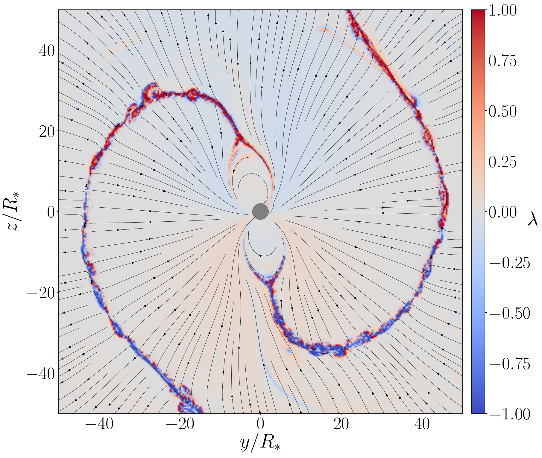
where . can be understood as the parallel force-free current in the corotating frame (Bai & Spitkovsky 2010, see, e.g.). We identify regions where as the current sheets (see Figure 3 for a map). We place emitter particles in these cells between . The motion of these particles consists of parallel motion along the magnetic field lines as well as drift in the azmuthal direction:
| (7) |
where is the direction of the magnetic field, is the drift velocity, and is a normalizing factor such that and the particle is moving outwards. We allow for a small emission cone for each particle of angular size , and the actual emission direction is taken from a Gaussian distribution centered around with width .
To produce the skymap where is the observation phase and is the observation angle, we subject the emission to the usual time delay (Bai & Spitkovsky 2010, e.g.,):
| (8) |
where is the azimuthal direction of the emission direction . We sum the contribution from each particle with a weight factor equal to , which place the emphasis on the current sheet as well as taking into account the local magnetic field.
To determine the dipole inclination , we ran a series of simulations with pure dipole magnetic field and vary from to . Figure 2 shows the skymaps and lightcurves from these simulations using the above prescription. Since we have a separate constraint on viewing angle from the NICER observations, we could use the positions of the two gamma-ray peaks as well as the amount of emission between peaks to determine the inclination angle. The comparison seems to indicate that . We chose which indeed gives a reasonable description for the observed lightcurve, as can be seen in the top panel of Figure 4.
IV Numerical Model for PSR J0030+0451
The final parameters we settle with are:
| (9) | ||||
| (10) | ||||
| (11) |
This set of parameters corresponds to a dipole inclination angle of . The quadrupole component is shifted and centered at .
Figure 3 shows a global view of the force-free magnetosphere. The force-free parameter is indeed small everywhere except in current sheets, providing a reliable way to identify them. The closed field lines remain similar to the vacuum configuration, whereas open field lines become mostly toroidal outside the light cylinder. These features agree with force-free simulations reported by Spitkovsky 2006, and kinetic simulations by Cerutti et al. 2016, Philippov & Spitkovsky 2018, and Kalapotharakos et al. 2018. The global magnetosphere also remains dipole-like, but the magnetospheric current is redirected to modified polar caps due to the presence of higher multipole fields, in agreement with the prediction by Gralla et al. 2017. Note that we did not include general relativistic corrections to , which will likely reduce and enhance (Philippov et al. 2015; Chen et al. 2020).
The bottom panel of Figure 3 shows the polar caps from both force-free and vacuum fields. The force-free polar caps are obtained by integrating open field lines towards the star. Since the simulation boundary condition is applied at , we use the vacuum field for the integration between . changes sign across both polar caps, and is either negative or larger than unity. Note that although the force-free polar caps closely resemble the vacuum ones, they are larger and slightly shifted. It is difficult to match the force-free polar caps directly with NICER results since a full fit using simulation results would take a prohibitive amount of computational resources.
Figure 4 shows a comparison of different lightcurves from our numerical model compared with the observations. The peaks of the numerical lightcurves naturally line up with the data, without the need to individually shift each component. In the rest of this section, we discuss our method to compute the radio and X-ray lightcurves from the simulation results.
IV.1 Radio Emission

To obtain the radio lightcurve, we adopt a prescription similar to the gamma-rays, and use equation (8) to compute the arrival phase of the signals emitted by test particles. Instead of identifying the emitting region using , we assume all open field lines between and a variable are emitting. We sum up all the emission in this region and vary to try to determine the likely radii for radio emission.
There still remains a significant degree of freedom in the weight we assign to each emitting particle. We attempted several different weighting schemes:
- •
Uniform emission weight.
- •
Particle emission weight is proportional to .
- •
For all the cells between and we define a mean emission direction by averaging the emission vector . The emission weight is proportional to where is the angle between the emission direction and the mean direction. This “ring-like” scheme emphasizes the emission at the edge of the polar caps.
- •
Similar as above, but weight proportional to . This “center” scheme emphasizes the geometric centers of the polar caps.
Figure 5 shows the results from the four schemes above. In general, we always produce two radio peaks, one large and one small, separated by approximately a half cycle. This is consistent with the observed pattern. It can be seen that in general larger leads to higher interpulse. For each scheme, the relative strengths of the two radio pulses single out an optimal . The scheme reflects the current structure of the polar caps, showing split patterns on the skymap, a direct result of the split polar caps shown in Figure 3. The ring-like weighting scheme does indeed show a ring-like pattern on the skymap, and tends to produce a double peak for the main radio peak. The center scheme does not produce an appreciable interpulse between the main peaks until . At this point both radio peaks are too wide and arrive systematically earlier than the observed ones. The weighting is the most physically motivated, since the magnetospheric current is what drives pair production (Beloborodov 2008; Timokhin & Arons 2013) and as a result, radio emission. We find the scheme with is closest to the observations (see middle panel of Figure 4).
The main radio peak in our best model is still wider than the observed one. We believe this is because we assume the whole open field line bundle is radio-emitting. Since this peak corresponds to the elongated polar cap, it is conceivable that at the two corners of the polar cap the parallel voltage is limited by the geometry, and pairs can only be produced in the central region of the polar cap, resulting in a much narrower radio-emitting region. This possibility needs to be investigated further using self-consistent simulations. We focus mostly on relatively large radii for radio emission, ignoring the relativistic light bending effect which is important for the X-rays. This effect may influence the contribution to the observed radio emission from lower altitudes .
IV.2 Hotspots and X-ray Lightcurve
We obtain the force-free polar caps by tracing open field lines back to . The resulting polar caps are close to the vacuum polar caps that we started with, which is a good consistency check. Both polar caps are split into halves with different signs of current flowing, reminiscent of near-orthogonal dipole rotators (Timokhin & Arons 2013, see, e.g.). In both polar caps, is either negative (anti-GJ) or larger than unity (super-GJ), suggesting that the whole polar cap should be active. As a first approximation, we simply assume that both polar caps are heated uniformly by the current flowing in the magnetosphere.
We construct the X-ray lightcurve using the X-PSI package developed by the Amsterdam group (Riley & Watts 2019) 44 4 https://github.com/ThomasEdwardRiley/xpsi. The current version of X-PSI lacks the ability to handle arbitrary-shaped hotspots. Instead, we discretized the two hotspots on a – grid, then put a small circular hotspot at the center of each occupied grid point with uniform temperature . The shape of the polar caps can be found in the bottom panel of Figure 3 (we used the FFE configuration). The stellar surface is taken to be cold () and does not contribute to the NICER observing band. This ensemble of circular hotspots is then fed into X-PSI to produce an ensemble of lightcurves. We sum all the lightcurves to produce the one shown in the bottom panel of Figure 4. Again as a consistency check, the lightcurve we obtained using this process is close to the observations.
V Conclusion
We presented a numerical model that can reasonably reproduce the lightcurves of PSR J0030+0451 at all observed frequencies including radio, X-ray, and gamma-ray (Figure 4). To achieve this, it is sufficient to include only up to quadrupole magnetic field near the star with an offset. We find that a dipole inclination angle of reproduces well the relative positions of the gamma-ray peaks.
The agreement of the new numerical model with observations strongly suggests that electric current is indeed the driving factor for the multi-wavelength emission in the pulsar magnetosphere. In addition, we developed a method to simultaneously compute radio and gamma-ray emission from a given magnetic field configuration using the force-free current ratio . The radio emission height we obtained are not inconsistent with the phenomenological calculations by Kijak & Gil 2003, suggesting that our recipe can be potentially applied to other pulsars as well.
The simulations presented in this Letter are limited in resolution due to our constraints on computation power. Future large-scale force-free simulations should be able to better resolve the star, with stellar surface at instead of . This will give a better representation of the current distribution on the stellar surface and better map to the configuration of hotspots. It could even be possible to perform direct Particle-in-cell simulations of J0030 in the foreseeable future, which will be able to pin-point the regions of dissipation in the magnetosphere. PIC simulations will be able to measure the amount of energy dissipated in the magnetosphere, and the fraction of it which goes to heat the stellar surface, explaining the origin and temperature of the hotspots on the star.
References
- Abdo et al. (2009) Abdo, A. A., Ackermann, M., Atwood, W. B., et al. 2009, ApJ, 699, 1171, doi: 10.1088/0004-637X/699/2/1171
- Abdo et al. (2013) Abdo, A. A., Ajello, M., Allafort, A., et al. 2013, ApJS, 208, 17, doi: 10.1088/0067-0049/208/2/17
- Bai & Spitkovsky (2010) Bai, X.-N., & Spitkovsky, A. 2010, ApJ, 715, 1282, doi: 10.1088/0004-637X/715/2/1282
- Beloborodov (2008) Beloborodov, A. M. 2008, ApJ, 683, L41, doi: 10.1086/590079
- Bilous et al. (2019) Bilous, A. V., Watts, A. L., Harding, A. K., et al. 2019, ApJ, 887, L23, doi: 10.3847/2041-8213/ab53e7
- Blandford (2002) Blandford, R. D. 2002, in Lighthouses of the Universe: The Most Luminous Celestial Objects and Their Use for Cosmology, ed. M. Gilfanov, R. Sunyeav, & E. Churazov, 381, doi: 10.1007/10856495_59
- Bogdanov et al. (2019) Bogdanov, S., Guillot, S., Ray, P. S., et al. 2019, ApJ, 887, L25, doi: 10.3847/2041-8213/ab53eb
- Carpenter & Kennedy (1994) Carpenter, M. H. K., & Kennedy, C. A. 1994, Fourth-order 2N-storage Runge-Kutta schemes, Technical Report NASA-TM-109112, NAS 1.15:109112, NASA Langley Research Center; Hampton, VA, United States. https://ntrs.nasa.gov/search.jsp?R=19940028444
- Cerutti et al. (2015) Cerutti, B., Philippov, A., Parfrey, K., & Spitkovsky, A. 2015, MNRAS, 448, 606, doi: 10.1093/mnras/stv042
- Cerutti et al. (2016) Cerutti, B., Philippov, A. A., & Spitkovsky, A. 2016, MNRAS, 457, 2401, doi: 10.1093/mnras/stw124
- Chen & Beloborodov (2014) Chen, A. Y., & Beloborodov, A. M. 2014, ApJ, 795, L22, doi: 10.1088/2041-8205/795/1/L22
- Chen et al. (2020) Chen, A. Y., Cruz, F., & Spitkovsky, A. 2020, ApJ, 889, 69, doi: 10.3847/1538-4357/ab5c20
- Dedner et al. (2002) Dedner, A., Kemm, F., Kröner, D., et al. 2002, Journal of Computational Physics, 175, 645, doi: 10.1006/jcph.2001.6961
- Dyks et al. (2004) Dyks, J., Harding, A. K., & Rudak, B. 2004, ApJ, 606, 1125, doi: 10.1086/383121
- East et al. (2015) East, W. E., Zrake, J., Yuan, Y., & Blandford, R. D. 2015, Phys. Rev. Lett., 115, 095002, doi: 10.1103/PhysRevLett.115.095002
- Gralla et al. (2017) Gralla, S. E., Lupsasca, A., & Philippov, A. 2017, ApJ, 851, 137, doi: 10.3847/1538-4357/aa978d
- Gruzinov (1999) Gruzinov, A. 1999, ArXiv e-prints, astro. https://arxiv.org/abs/astro-ph/9902288
- Gruzinov (2006) —. 2006, ApJ, 647, L119, doi: 10.1086/506590
- Hakobyan et al. (2019) Hakobyan, H., Philippov, A., & Spitkovsky, A. 2019, ApJ, 877, 53, doi: 10.3847/1538-4357/ab191b
- Johnson et al. (2014) Johnson, T. J., Venter, C., Harding, A. K., et al. 2014, ApJS, 213, 6, doi: 10.1088/0067-0049/213/1/6
- Kalapotharakos et al. (2018) Kalapotharakos, C., Brambilla, G., Timokhin, A., Harding, A. K., & Kazanas, D. 2018, ApJ, 857, 44, doi: 10.3847/1538-4357/aab550
- Kijak & Gil (2003) Kijak, J., & Gil, J. 2003, A&A, 397, 969, doi: 10.1051/0004-6361:20021583
- Kreiss & Oliger (1973) Kreiss, H. O., & Oliger, J. 1973, Methods for the approximate solution of time dependent problems, GARP publications series No. 10 (Geneva: Global Atmospheric Research Programme - WMO-ICSU Joint Organizing Committee)
- Lockhart et al. (2019) Lockhart, W., Gralla, S. E., Özel, F., & Psaltis, D. 2019, MNRAS, 490, 1774, doi: 10.1093/mnras/stz2524
- Miller et al. (2019) Miller, M. C., Lamb, F. K., Dittmann, A. J., et al. 2019, ApJ, 887, L24, doi: 10.3847/2041-8213/ab50c5
- Philippov et al. (2015) Philippov, A. A., Cerutti, B., Tchekhovskoy, A., & Spitkovsky, A. 2015, ApJ, 815, L19, doi: 10.1088/2041-8205/815/2/L19
- Philippov & Spitkovsky (2018) Philippov, A. A., & Spitkovsky, A. 2018, ApJ, 855, 94, doi: 10.3847/1538-4357/aaabbc
- Riley et al. (2019) Riley, T. E., Watts, A. L., Bogdanov, S., et al. 2019, ApJ, 887, L21, doi: 10.3847/2041-8213/ab481c
- Spitkovsky (2006) Spitkovsky, A. 2006, ApJ, 648, L51, doi: 10.1086/507518
- Timokhin & Arons (2013) Timokhin, A. N., & Arons, J. 2013, MNRAS, 429, 20, doi: 10.1093/mnras/sts298
- Yuan et al. (2019) Yuan, Y., Spitkovsky, A., Blandford, R. D., & Wilkins, D. R. 2019, MNRAS, 487, 4114, doi: 10.1093/mnras/stz1599
- Zrake & East (2016) Zrake, J., & East, W. E. 2016, ApJ, 817, 89, doi: 10.3847/0004-637X/817/2/89