Active Set Expansion Strategies in MPRGP Algorithm

As our experiments demonstrate, it is better to perform longer steps which are often unfeasible and to make a subsequent projection onto the feasible set. One of the ideas how to choose these longer steps comes from the steepest descent method. We analyze the step lengths in a given direction to find a step length for which the cost function decrease is maximal. As our cost function is parabolic, we can guarantee the cost function decrease with up to twice the optimal step length.

Let us reiterate that our cost function is

and that the expansion does a step in the $\bm{g}^{r}$ direction with a fixed step length $\overline{\alpha}\in(0,2||\bm{A}||^{-1}]$. Let us assume that we do a step in a direction $\bm{d}$ instead, where $\bm{d}$ is either $\bm{g}^{r}$ or $\bm{g}^{f}$ so that no active component is freed. We want to choose a step length such that the cost function decreases, i.e.,

and after division by $\bar{\alpha}>0$

Assuming $\bm{d}$ is not in the null space of $\bm{A}$, we have $\bm{d}^{T}\bm{Ad}>0$ and so we can divide the inequality by $\bm{d}^{T}\bm{A}\bm{d}$

Because $\bm{d}$ is either free gradient or reduced free gradient, we have

so that

We know that

that proves

Furthermore

which gives us a larger upper bound for $\bar{\alpha}$

We can consider this bound

as an adaptive step length for an expansion step taking into account the actual situation. For testing, let us consider the following notation:

• 1.

  fixed $\bar{\alpha}=\alpha_{u}\left\|\bm{A}\right\|^{-1},$

• 2.

  optapprox $\bar{\alpha}=\alpha_{u}\left\|\bm{A}\right\|^{-1}\frac{\bm{d}^{T}\bm{g}}{\bm{d}^{T}\bm{d}},$

• 3.

  opt $\bar{\alpha}=\alpha_{u}\frac{\bm{d}^{T}\bm{g}}{\bm{d}^{T}\bm{A}\bm{d}}$,

where $\alpha_{u}\in(0,2]$. Any choice of the $\overline{\alpha}$ from the above options guarantees the reduction of the cost function. However, only the fixed choice of $\overline{\alpha}$ and descent direction $\bm{d}=\bm{g}^{r}$ ensures that $\bm{x}$ is kept in the feasible set. Therefore, we need to project the new approximation to the feasible set, i.e,

The above expression is exactly the expansion step of the original algorithm with $\tilde{\bm{d}}=\bm{g}^{f}$. Since we derived the step lengths without taking into considerations the projection, it makes sense to decouple the $\bm{d}$ used for computation of $\overline{\alpha}$ and the descent direction $\tilde{\bm{d}}$.

Note that some combinations of vectors used for step length computation as well as descent directions are equivalent. Namely, fixed step length is equivalent to optapprox with $\bm{d}=\bm{g}^{f}$ with any of the two descent directions.

Recall, that the expansion consists of the half step followed by the expansion step line search. The half step is a CG step with step length reduced such that the computed approximation is in the feasible set.

Since our goal is to expand the active set faster, it seems reasonable to replace the half step by the full CG step with a subsequent projection onto the feasible set. To be more specific, our expansion step becomes

followed by reseting $\bm{p}=\bm{g}^{f}$. Note, that realising the expansion in this way simplifies the implementation as we can always compute the CG step and then compute the gradient using CG recurrence when the step was feasible; otherwise, we project the solution onto the feasible set and recompute the gradient explicitly. Algorithm 5 illustrates the implementation. It replaces if…else block on lines 6–9 in Algorithm 1.

However, in some cases, this step can lead to an increase in the cost function. In [3], section 6.2, the author illustrates by Figure 1 the situation when increase in the cost function happens. Clearly, the CG step finds the uncostrained minimizer of the cost function, but the subsequent projection onto the feasible set puts as on a higher contour line, i.e., increases the value of cost function. In this case the standard expansion would put as closer to solution. Yet, unless $\overline{\alpha}$ happens to be such that the line search finds the exact solution, both approaches converge in the next iteration. Note that in this example, opt step length with $\alpha_{u}=1$ with any combination of the allowed vector for both the compuation of the step length and line search direction would converge to the exact solution in a single iteration.

Let us consider the a spatial domain $\Omega$ which is decomposed into non-overlapping subdomains. Then virtually arbitrary Finite Element Method (FEM) implementation can be used to generate the subdomain stiffness matrices $\bm{K}_{s}$ and the subdomain load vectors $\bm{f}_{s}$ as sequential data for each subdomain $\Omega_{s}$, $s=1,\,\ldots,\,N_{S}$ independently.

The original primal problem

where $\bm{K}=diag(\bm{K}_{1},\dots,\bm{K}_{N_{S}})$ is global stiffness matrix, $\bm{f}=\left[\bm{f}_{1}^{T},\dots,\bm{f}_{N_{S}}^{T}\right]^{T}$ is global right hand side, $\bm{u}$ is unknown displacement, $\bm{B}_{I}$ represents non-penetration condition, and $\bm{B}_{E}$ glues the subdomains together. The primal problem is transformed into dual one

where

$\bm{K}^{\dagger}$ denotes a left generalized inverse of $\bm{K}$, i.e. a matrix satisfying $\bm{K}\bm{K}^{\dagger}\bm{K}=\bm{K}$ and columns of $\bm{R}$ span the null space. The constraint matrix $\bm{B}=\left[\begin{smallmatrix}\bm{B}_{I}^{T}&\bm{B}_{E}^{T}\end{smallmatrix}\right]^{T}$ can be constructed so that it has a full rank, and then the Hessian $\bm{F}$ is positive definite with a relatively favourably distributed spectrum for application of the CG method. For more details see …

Support Vector Machines (SVMs) belong to the conventional machine learning (ML) techniques, and they can solve classification as well as regression problems. Despite the fact that deep learning (DL) [10] is getting popular in the recent years, SVMs are successfully applied for specific tasks in various scientific areas including genetics [11], geosciences [12], and image analysis [13]. Unlike the DL underlying architecture, SVMs could be considered as the single perceptron problems that find the learning functions that maximize the geometric margins. Therefore, we can simply explain the qualities of a learning model and the underlying solver behaviour. In this paper, we will focus on the linear SVMs for classifications.

SVM was originally designed as a supervised binary classifier [14], i.e., a classifier that decides whether a sample falls into either Class A or Class B employing a model determined from already categorised samples in the training phase of the classifier. Let us denote the training data as an ordered sample-label pairs such that

where $m$ is the number of samples, $\bm{x}_{i}\in\mathbb{R}^{n},\ n\in\mathbb{N},$ is the $i$-th sample and $y_{i}\in\{-1,1\}$ denotes the label of the $i$-th sample, $i\in\{1,\ 2,\ \dots,m\}$. The label determines the sample’s class.

Standard SVM solves problem of finding a classification model in a form of maximal-margin hyperplane $H=\left\langle\bm{w},\bm{x}\right\rangle+b$, where $\bm{w}$ is the normal vector of the hyperplane $H$ and $b$ is its bias from origin. In the no-bias classification, we do not consider bias $b$ in a classification model, but we include it into the problem by means of augmenting the vector $\bm{w}$ and each sample $\bm{x}_{i}$ with an additional dimension so that $\bm{\widehat{w}}\leftarrow\begin{bmatrix}\bm{w}\\ b\end{bmatrix}$, $\bm{\widehat{x}_{i}}\leftarrow\begin{bmatrix}\bm{x}_{i}\\ \beta\end{bmatrix}$, where $\beta\in\mathbb{R}^{+}$ is a user defined variable (typically set to $1$).

The problem of finding hyperplane $\widehat{H}=\left\langle\bm{\widehat{w}},\bm{\widehat{x}}\right\rangle$ can be formulated as a constrained optimization problem in the following primal formulation

where $p\in\{1,2\}$, $\xi_{i}=\max\left(0,1-y_{i}\left\langle\bm{\widehat{w}},\bm{\widehat{x}}_{i}\right\rangle\right)$ is the hinge loss function and $C\in\mathbb{R}^{+}$ is a user defined penalty. Using the Lagrange duality and denoting $\bm{H}=\bm{Y}^{T}\bm{G}\bm{Y}$, $\bm{Y}=diag(\bm{y})$, $\bm{y}=\left[y_{1},\ y_{2},\ \dots,y_{m}\right]^{T}$, $\bm{G}=\bm{X}^{T}\bm{X}$, $\bm{X}=\begin{bmatrix}\bm{\widehat{x}}_{1}&\dots&\bm{\widehat{x}}_{m}\end{bmatrix}$, $\bm{e}=\left[1,1,\dots,1\right]^{T}\in\mathbb{R}^{m}$, $\bm{o}=\left[0,\ 0,\ \dots,\ 0\right]^{T}\in\mathbb{R}^{m}$ , we transform (6) into the dual formulations

for $p=1$ and

for $p=2$. The first formulation is commonly called dual $l1$-loss SVM, and the second one is known as dual $l2$-loss SVM. The Hessian associated with QP problem (7) is symmetric positive-semi definite. It becomes positive definite using regularization by matrix $C^{-1}\bm{I}$ in formulation (8).

The first benchmark is a 3D linear elasticity contact problem. We considered an elastic cube with the dimensions $1\times 1\times 1$ [mm] with the bottom face fixed, the top one loaded with a vertical surface force $f_{z}=-465$ [N/mm²] directed downwards, and the right one in contact with a rigid obstacle. Young modulus is $E=2\cdot 10^{5}$ [MPa] and Poisson ratio $\mu=0.33$. See Figure 2.

We use TFETI domain decomposition to solve this problem. Let us consider only one regular decomposition into 1000 subdomains (10 in each direction) with 27,000 elements per subdomains (30 in each direction) making a total of 81,812,703 (undecomposed) degrees of freedom. We use M-variant of the SMALBE [1] algorithm to take care of the equality constraint with MPRGP used as the inner solver. The stopping tolerance of the outer solver (SMALBE) is set to $10^{-6}$ relative to the right-hand side. Other parameters for SMALBE are $M=100||\bm{A}||$, $\eta=1.1||\bm{A}||$ and, when the decrease of the Lagrangian is sufficient, $M$ is reduced by $10$.

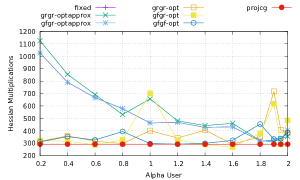
Results, in term of the overall number of Hessian multiplications are reported in Figure 3. Note, that the projected CG expansion variant does not contain parametr $\alpha_{u}$. Table 2 compares the numbers of outer and inner iterations, i.e. numbers of CG, expansion, proportioning steps and Hessian multiplications for the three best values of $\alpha_{u}$. The full results are reported in A.

The standard expansion with the fixed-length expansion step needs $318$ Hessian multiplication for the best $\alpha_{u}=1.8$. The number of Hessian multiplications mostly decreases until the best $\alpha_{u}$ is reached and then starts to increase again.

The optapprox variants do not bring much as they achieve the convergence in a very similar number of iterations to the fixed variant. This behaviour suggests that the free gradient is not sufficiently different from the reduced free gradient, i.e., $\bm{g}^{f}\approx\bm{g}^{r}$ and we have

Much better are the opt step lengths. They can significantly decrease the number of expansion steps needed (up to half in one case). The number of Hessian multiplications is decreased as well, but due to the additional Hessian multiplication, the effect is less pronounced. The best result of $269$ Hessian multiplication achieved step length computed with $\bm{g}^{r}$ in the direction of $\bm{g}^{f}$ for $\alpha_{u}=1.6$, a decrease of $15\%$ compared to the best fixed variant). The other variants of opt outperformed fixed as well, requiring $292$ Hessian multiplication (reduction of $8\%)$. The problem with any of the opt strategies is that there are quite large jumps in the number of Hessian multiplications depending on the value of $\alpha_{u}$.

Lastly, the project CG step variant of expansion performs well. It achieves $292$ Hessian multiplication, a reduction of $8\%$ compared to fixed. Moreover, it is outperformed only by the best opt strategy, but there is no dependence on the $\alpha_{u}$.

The second benchmark uses SVMs for classifications on three publicly available datasets, namely Australian, Diabetes, and Ionosphere downloaded from LIBSVM dataset webpage [15]. The Australian dataset (Australian Credit Approval) concerns credit card applications. The objective of the Diabetes dataset is to predict whether a patient has diabetes. Finally, the Ionosphere dataset is about the classification of radar returns from the ionosphere as either suitable for further analysis or not. The information about the number of samples and features for each dataset are in Table 3.

We use the no-bias SVM formulation with $l1$ hinge-loss fuction and with $C=1$. Since this is a classification application, there are very low requirements on the accuracy of the underlying solver [9]. Therefore, the relative tolerance of MPRGP is set to $10^{-1}$. The initial guess is set just under the upper bound (each component is set to $1-100\epsilon_{m}$, where $\epsilon_{m}\approx 2.2\mathrm{e}{-16}$ is the machine epsilon).

As in the previous bechmark, we report the results in term of the overall number of Hessian multiplications in Figures 4, 5, and 6. Note that we removed an outlier from the Ionosphere dataset graph; for gfgr-opt with $\alpha_{u}=1.9$ there was a total of $2,322$ Hessian multiplications required for convergence. In Tables 4, 5, and 6 the number of CG, expansion, proportioning steps and Hessian multiplications are compared for the three best values of $\alpha_{u}=1.9$. The full results are reported in A.

For each dataset, the default expansion with the fixed step length achieves the best performance for $\alpha_{u}\approx 1.9$. The best fixed strategy converged in $195$, $615$, and $380$ Hessian multiplications for Australian, Diabetes, and Ionosphere datasets, respectively.

As in the previous benchmark, the optapprox strategy is quite close to the fixed step length.

For the Australian dataset, the best opt variant was gfgr for $\alpha_{u}=1.4$ which was closely followed by gfgf for $\alpha_{u}=2.0$. Moreover, gfgf with the same value of $\alpha_{u}$ was the best variant for the other datasets. Comparing, for the best opt strategy, the number of Hessian multiplication with fixed we have $101$ (reduction of $48\%$) for Australian, $134$ (reduction of $78\%$) for Diabetes, $113$ (reduction of $70\%$) for Ionosphere.

The projcg strategy performed the best for both Australian and Diabetes dataset. It was the second-best from all results for the Ionosphere dataset. Againg comparing the number of Hessian multiplication with fixed we have $83$ (reduction of $57\%$) for Australian, $133$ (reduction of $78\%$) for Diabetes, $125$ (reduction of $67\%$) for Ionosphere.

References

- [1] Z. Dostál, Optimal Quadratic Programming Algorithms, with Applications to Variational Inequalities, Volume 23, SOIA, Springer, New York, US, 2009.
- [2] V. Hapla, et al., “PERMON (Parallel, Efficient, Robust, Modular, Object-oriented, Numerical)”, http://permon.it4i.cz.
- [3] Z. Dostál, T. Kozubek, M. Sadowská, V. Vondrák, Scalable Algorithms for Contact Problems, Advances in Mechanics and Mathematics. Springer New York, 2017, ISBN 9781493968329.
- [4] V. Hapla, D. Horák, L. Pospíšil, M. Čermák, A. Vašatová, R. Sojka, “Solving Contact Mechanics Problems with PERMON”, in High Performance Computing in Science and Engineering, Volume 9611 of Lecture Notes in Computer Science, pages 101–115. Springer International Publishing Switzerland, 2016, ISBN 978-3-319-40361-8, ISSN 0302-9743.
- [5] S. Balay, S. Abhyankar, M.F. Adams, J. Brown, P. Brune, K. Buschelman, L. Dalcin, A. Dener, V. Eijkhout, W.D. Gropp, D. Kaushik, M.G. Knepley, D.A. May, L.C. McInnes, R.T. Mills, T. Munson, K. Rupp, P. Sanan, B.F. Smith, S. Zampini, H. Zhang, H. Zhang, “PETSc Web page”, http://www.mcs.anl.gov/petsc, 2018, URL http://www.mcs.anl.gov/petsc.
- [6] S. Balay, S. Abhyankar, M.F. Adams, J. Brown, P. Brune, K. Buschelman, L. Dalcin, A. Dener, V. Eijkhout, W.D. Gropp, D. Kaushik, M.G. Knepley, D.A. May, L.C. McInnes, R.T. Mills, T. Munson, K. Rupp, P. Sanan, B.F. Smith, S. Zampini, H. Zhang, H. Zhang, “PETSc Users Manual”, Technical Report ANL-95/11 - Revision 3.10, Argonne National Laboratory, 2018, URL http://www.mcs.anl.gov/petsc.
- [7] A. Dener, A. Denchfield, T. Munson, J. Sarich, S. Wild, S. Benson, L.C. McInnes, “TAO Users Manual”, Technical Report ANL/MCS-TM-322 Rev. 3.10, Argonne National Laboratory, 2018.
- [8] V. Hapla, D. Horák, M. Pecha, “PermonSVM”, 2017, URL http://permon.vsb.cz/permonsvm.htm.
- [9] J. Kružík, M. Pecha, V. Hapla, D. Horák, M. Čermák, “Investigating convergence of linear SVM implemented in PermonSVM employing MPRGP algorithm”, Volume 11087 LNCS of Lecture Notes in Computer Science (including subseries Lecture Notes in Artificial Intelligence and Lecture Notes in Bioinformatics), pages 115–129, 2018.
- [10] Y. LeCun, Y. Bengio, G. Hinton, “Deep learning”, nature, 521(7553): 436, 2015.
- [11] M. Brown, W. Grundy, D. Lin, N. Cristianini, C. Sugnet, T. Furey, M. Ares Jr., D. Haussler, “Knowledge-based analysis of microarray gene expression data by using support vector machines”, Proceedings of the National Academy of Sciences of the United States of America, 97(1): 262–267, 2000.
- [12] J. Shi, W.J. Lee, Y. Liu, Y. Yang, P. Wang, “Forecasting power output of photovoltaic systems based on weather classification and support vector machines”, IEEE Transactions on Industry Applications, 48(3): 1064–1069, 2012.
- [13] G.M. Foody, A. Mathur, “The use of small training sets containing mixed pixels for accurate hard image classification: Training on mixed spectral responses for classification by a SVM”, Remote Sensing of Environment, 103(2): 179 – 189, 2006, ISSN 0034-4257.
- [14] C. Cortes, V. Vapnik, “Support-Vector Networks”, Machine Learning, 20(3): 273–297, Sept. 1995, ISSN 0885-6125.
- [15] “LIBSVM Data: Classification (Binary Class)”, URL https://www.csie.ntu.edu.tw/˜cjlin/libsvmtools/datasets/binary.html.
Appendix A Full Numerical Results