Adversarial Distributional Training for
Robust Deep Learning
Abstract
Adversarial training (AT) is among the most effective techniques to improve model robustness by augmenting training data with adversarial examples. However, most existing AT methods adopt a specific attack to craft adversarial examples, leading to the unreliable robustness against other unseen attacks. Besides, a single attack algorithm could be insufficient to explore the space of perturbations. In this paper, we introduce adversarial distributional training (ADT), a novel framework for learning robust models. ADT is formulated as a minimax optimization problem, where the inner maximization aims to learn an adversarial distribution to characterize the potential adversarial examples around a natural one under an entropic regularizer, and the outer minimization aims to train robust models by minimizing the expected loss over the worst-case adversarial distributions. Through a theoretical analysis, we develop a general algorithm for solving ADT, and present three approaches for parameterizing the adversarial distributions, ranging from the typical Gaussian distributions to the flexible implicit ones. Empirical results on several benchmarks validate the effectiveness of ADT compared with the state-of-the-art AT methods.
1 Introduction
While recent breakthroughs in deep neural networks (DNNs) have led to substantial success in a wide range of fields [21], DNNs also exhibit adversarial vulnerability to small perturbations around the input [62, 22]. Due to the security threat, considerable efforts have been devoted to improving the adversarial robustness of DNNs [22, 38, 40, 44, 70, 48, 74, 49, 80]. Among them, adversarial training (AT) is one of the most effective techniques [2, 16]. AT can be formulated as a minimax optimization problem [44], where the inner maximization aims to find an adversarial example that maximizes the classification loss for a natural one, while the outer minimization aims to train a robust classifier using the generated adversarial examples. To solve the non-concave and typically intractable inner maximization problem approximately, several adversarial attack methods can be adopted, such as fast gradient sign method (FGSM) [22] and projected gradient descent (PGD) method [44].
However, existing AT methods usually solve the inner maximization problem based on a specific attack algorithm, some of which can result in poor generalization for other unseen attacks under the same threat model [60]11 1 It should be noted that we consider the generalization problem across attacks under the same threat model, rather than studying the generalization ability across different threat models [25, 17, 64].. For example, defenses trained on the FGSM adversarial examples, without random initialization or early stopping [71], are vulnerable to multi-step attacks [38, 65]. Afterwards, recent methods [79, 72] can achieve the state-of-the-art robustness against the commonly used attacks (e.g., PGD), but they can still be defeated by others [41, 66]. It indicates that these defenses probably cause gradient masking [65, 2, 68], and can be fooled by stronger or adaptive attacks.
Moreover, a single attack algorithm could be insufficient to explore the space of possible perturbations. PGD addresses this issue by using random initialization, however the adversarial examples crafted by PGD with random restarts probably lie together and lose diversity [63]. As one key to the success of AT is how to solve the inner maximization problem, other methods perform training against multiple adversaries [65, 30], which can be seen as more exhaustive approximations of the inner problem [44]. Nevertheless, there still lacks a formal characterization of multiple, diverse adversaries.
To mitigate the aforementioned issues and improve the model robustness against a wide range of adversarial attacks, in this paper we present adversarial distributional training (ADT), a novel framework that explicitly models the adversarial examples around a natural input using a distribution. Subsuming AT as a special case, ADT is formulated as a minimax problem, where the inner maximization aims to find an adversarial distribution for each natural example by maximizing the expected loss over this distribution, while the outer minimization aims to learn a robust classifier by minimizing the expected loss over the worst-case adversarial distributions. To keep the adversarial distribution from collapsing into a Delta one, we explicitly add an entropic regularization term into the objective, making the distribution capable of characterizing heterogeneous adversarial examples.
Through a theoretical analysis, we show that the minimax problem of ADT can be solved sequentially similar to AT [44]. We implement ADT by parameterizing the adversarial distributions with trainable parameters, with three concrete examples ranging from the classical Gaussian distributions to the very flexible implicit density models. Extensive experiments on the CIFAR-10 [36], CIFAR-100 [36], and SVHN [46] datasets validate the effectiveness of our proposed methods on building robust deep learning models, compared with the alternative state-of-the-art AT methods.
2 Proposed method
In this section, we first introduce the background of adversarial training (AT), then detail adversarial distributional training (ADT) framework, and finally provide a general algorithm for solving ADT.
2.1 Adversarial training
Adversarial training has been widely studied to improve the adversarial robustness of DNNs. Given a dataset of training samples with and being the natural example and the true label, AT can be formulated as a minimax optimization problem [44] as
| (1) |
where is the DNN model with parameters that outputs predicted probabilities over all classes, is a loss function (e.g., cross-entropy loss), and is a perturbation set with . This is the threat model widely studied before and what we consider in this paper. Our method can also be extended to other threat models (e.g., norm), which we leave to future work.
This minimax problem is usually solved sequentially, i.e., adversarial examples are crafted by solving the inner maximization first, and then the model parameters are optimized based on the generated adversarial examples. Several attack methods can be used to solve the inner maximization problem approximately, such as FGSM [22] or PGD [44]. For example, PGD takes multiple gradient steps as
| (2) |
where is the adversarial perturbation at the -th step, is the projection function, and is a small step size. is initialized uniformly in . will converge to a local maximum eventually.
2.2 Adversarial distributional training
As we discussed, though effective, AT is not problemless. AT with a specific attack possibly leads to overfitting on the attack pattern [38, 65, 79, 72], which hinders the trained models from defending against other attacks. And a single attack algorithm may be unable to explore all possible perturbations in the high-dimensional space, which could result in unsatisfactory robustness performance [65, 30].
To alleviate these problems, we propose to capture the distribution of adversarial perturbations around each input instead of only finding a locally most adversarial point for more generalizable adversarial training, called adversarial distributional training (ADT). In particular, we model the adversarial perturbations around each natural example by a distribution , whose support is contained in . Based on this, ADT is formulated as a distribution-based minimax optimization problem as
| (3) |
where is a set of distributions with support contained in . As can be seen in Eq. (3), the inner maximization aims to learn an adversarial distribution, such that a point drawn from it is likely an adversarial example. And the objective of the outer minimization is to adversarially train the model parameters by minimizing the expected loss over the worst-case adversarial distributions induced by the inner problem. It is noteworthy that AT is a special case of ADT, by specifying the distribution family to contain Delta distributions only.
Regularizing adversarial distributions. For the inner maximization of ADT, we can easily see that
| (4) |
It indicates that the optimal distribution by solving the inner problem of ADT will degenerate into a Dirac one. Hence the adversarial distribution cannot cover a diverse set of adversarial examples, and ADT becomes AT. To solve this issue, we add an entropic regularization term into the objective as
| (5) |
where is the entropy of , is a balancing hyperparameter, and denotes the overall loss function for notation simplicity. Note that the entropy maximization is a common technique to increase the support of a distribution in generative modeling [12, 13] or reinforcement learning [23]. We next discuss why ADT is superior to AT.

2.2.1 Discussion on the superiority of ADT
The major difference between AT and ADT is that for each natural input , AT finds a worst-case adversarial example, while ADT learns a worst-case adversarial distribution comprising a variety of adversarial examples. Because adversarial examples can be generated by various attacks, we expect that those adversarial examples probably lie in the region where the adversarial distribution assigns high probabilities, such that minimizing the expected loss over this distribution can naturally lead to a better generalization ability of the trained classifier across attacks under the same threat model.
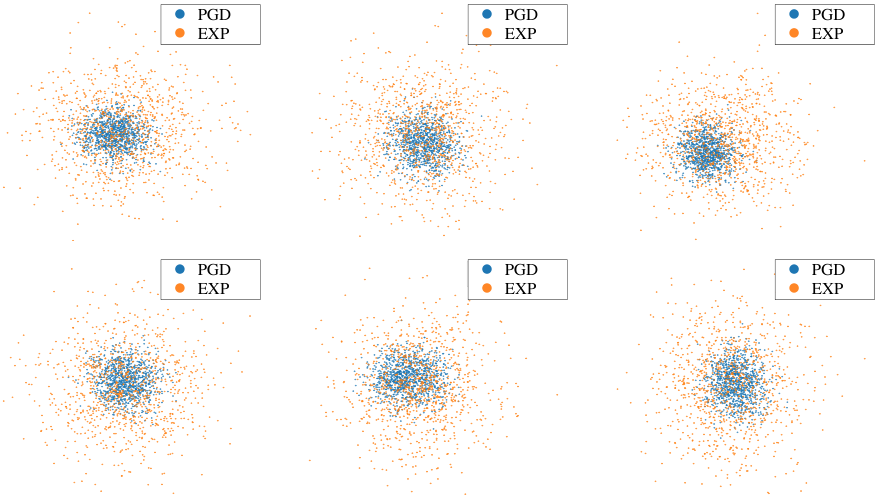
Furthermore, as we add an entropic regularizer into the objective (5), the adversarial distribution is able to better explore the space of possible perturbations and characterize more diverse adversarial examples compared with a single attack method (e.g., PGD). To show this, for each data we generate a set of adversarial examples by PGD with random restarts and sample another set of adversarial examples from the adversarial distribution learned by ADTEXP (a variant of ADT detailed in Sec. 3.1), targeted at a standard trained model. Then we can visualize these adversarial examples by projecting them onto the 2D space spanned by the first two eigenvectors given by PCA [32]. The visualization results of some randomly selected data points in Fig. 2 show that adversarial examples sampled from the adversarial distribution are scattered while those crafted by PGD concentrate together. We further evaluate the diversity of adversarial examples by quantitatively measuring their average pairwise distances. The average distance of adversarial examples sampled from the adversarial distribution over test images is , which is for PGD. Although the adversarial distributions can characterize more diverse adversarial examples, they have a similar attack power compared with PGD, as later shown in Table 4. Minimizing the loss on such diverse adversarial examples can consequently help to learn a smoother and more flattened loss surface around the natural examples in the input space, as shown in Fig. 2. Therefore, ADT can improve the overall robustness compared with AT.
2.3 A general algorithm for ADT
To solve minimax problems, Danskin’s theorem [14] states how the maximizers of the inner problem can be used to define the gradients for the outer problem, which is also the theoretical foundation of AT [44]. However, it is problematic to directly apply Danskin’s theorem for solving ADT since the search space may not be compact, which is one assumption of this theorem. As it is non-trivial to perform a theoretical analysis on how to solve ADT, we first lay out the following assumptions.
Assumption 1.
The loss function is continuously differentiable w.r.t. .
Assumption 1 is also made in [44] for AT. Although the loss function is not completely continuously differentiable due to the ReLU layers, the set of discontinuous points has measure zero, such that it is assumed not to be an issue in practice [44].
Assumption 2.
Probability density functions of distributions in are bounded and equicontinuous.
Assumption 2 puts a restriction on the set of distributions . We show that the explicit adversarial distributions proposed in Sec. 3.1 satisfy this assumption (in Appendix B.1).
Theorem 1.
The complete proof of Theorem 1 is deferred to Appendix B.1. Theorem 1 provides us a general principle for training ADT, by first solving the inner problem and then updating the model parameters along the gradient direction of the loss function at the global maximizer of the inner problem, in a sequential manner similar to AT [44]. We provide the general algorithm for ADT in Alg. 1. Analogous to AT, the global maximizer of the inner problem cannot be solved analytically. Therefore, we propose three different approaches to obtain approximate solutions, as introduced in Sec. 3. Although we cannot reach the global maximizer of the inner problem, our experiments suggest that we can reliably solve the minimax problem (5) by our algorithm.
3 Parameterizing adversarial distributions
At the core of ADT lie the solutions of the inner maximization problem of Eq. (5). The basic idea is to parameterize the adversarial distributions with trainable parameters . With the parameterized , the inner problem is converted into maximizing the expected loss w.r.t. . In the following, we present the parametrizations and learning strategies of three different approaches, respectively. We provide an overview of these approaches in Fig. 3.
3.1 ADTEXP: explicit modeling of adversarial perturbations
A natural way to model adversarial perturbations around an input data is using a distribution with an explicit density function. We name ADT with EXPlicit adversarial distributions as ADTEXP. To define a proper distribution on , we take the transformation of random variable approach as
| (8) |
where is sampled from a diagonal Gaussian distribution with as the mean and standard deviation. is transformed by a function and then multiplied by to get . We let denote the parameters to be learned. We sample from a diagonal Gaussian mainly for the sake of computational simplicity. But our method is fully compatible with more expressive distributions, such as matrix-variate Gaussians [42] or multiplicative normalizing flows [43], and we leave using them to future work. Given Eq. (8), the inner problem of Eq. (5) becomes
| (9) |
To solve this, we need to estimate the gradient of the expected loss w.r.t. the parameters . A commonly used method is the low-variance reparameterization trick [35, 5], which replaces the sampling process of the random variable of interest with the corresponding differentiable transformation. With this technique, the gradient can be back-propagated from the samples to the distribution parameters directly. In our case, we reparameterize by , where is an auxiliary noise variable following the standard Gaussian distribution . Therefore, we can estimate the gradient of via
| (10) |
The first term inside is the classification loss with the sampled noise, and the second is the negative log density (i.e., estimation of entropy). It can be calculated analytically (proof in Appendix B.2) as
| (11) |
where the superscript denotes the -th element of a vector.
In practice, we approximate the expectation in Eq. (10) with Monte Carlo (MC) samples, and perform steps of gradient ascent on to solve the inner problem. After obtaining the optimal parameters , we use the adversarial distribution to update model parameters .
3.2 ADTEXP-AM: amortizing the explicit adversarial distributions
Although the aforementioned method in Sec. 3.1 provides a simple way to learn explicit adversarial distributions for ADT, it needs to learn the distribution parameters for each input and then brings prohibitive computational cost. Compared with PGD-based AT which constructs adversarial examples by steps PGD [44], ADTEXP is approximately times slower since the gradient of is estimated by MC samples in each step. In this subsection, we propose to amortize the inner optimization of ADTEXP, to develop a more feasible and scalable training method. We name ADT with the AMortized version of EXPlicit adversarial distributions as ADTEXP-AM.
Instead of learning the distribution parameters for each data , we opt to learn a mapping , which defines the adversarial distribution for each input in a conditional manner . We instantiate by a conditional generator network. It takes a natural example as input, and outputs the parameters of its corresponding explicit adversarial distribution, which is also defined by Eq. (8). The advantage of this method is that the generator network can potentially learn common structures of the adversarial perturbations, which can generalize to other training samples [3, 51]. It means that we do not need to optimize excessively on each data , which can accelerate training.
3.3 ADTIMP-AM: implicit modeling of adversarial perturbations
Since the underlying distributions of adversarial perturbations have not been figured out yet and could be different across samples, it is hard to specify a proper explicit distribution of adversarial examples, which may lead to the underfitting problem. To bypass this, we resort to implicit distributions (i.e., distributions without tractable probability density functions but can still be sampled from), which have shown promising results recently [20, 57, 58], particularly in modeling complex high-dimensional data [53, 29]. The major advantage of implicit distributions is that they are not confined to provide explicit densities, which improves the flexibility inside the sampling process.
Based on this, we propose to use the implicit distributions to characterize the adversarial perturbations. Considering the priority of amortized optimization, we learn a generator which implicitly defines a conditional distribution by , where is a natural input and is a random noise vector. Typically, is sampled from a prior such as the standard Gaussian or uniform distributions as in the generative adversarial networks (GANs) [20]. In this work, we sample from a uniform distribution . We refer to this approach as ADTIMP-AM. A practical problem remains unaddressed is that the entropy of the implicit distributions cannot be estimated exactly as we have no access to the density . We instead maximize the variational lower bound of the entropy [12] for its simplicity and success in GANs [13]. We provide full technical details of ADTEXP-AM and ADTIMP-AM, and training algorithms of the three methods in Appendix A.
4 Related work
Adversarial machine learning is an emerging research topic with various attack and defense methods being proposed [22, 37, 6, 15, 40, 44, 70, 10, 49]. Besides PGD-based AT [44], recent improvements upon it include designing new losses [80, 45, 50, 52] or network architecture [74], accelerating the training procedure [56, 78, 71], and exploiting more data [26, 1, 8, 77].
Learning the distributions of adversarial examples has been studied before, mainly for black-box adversarial attacks. An adversarial example can be searched over a distribution [27, 39], similar to the inner problem of Eq. (3). But their gradient estimator based on natural evolution strategy exhibits very high variance [35] compared with ours in Eq. (10), since our methods are based on the white-box setting (i.e., compute the gradient) rather than the black-box setting. To the best of our knowledge, we are the first to train robust models by learning the adversarial distributions.
In this work, we adopt a generator network to amortize the adversarial distributions for accelerating the training process. There also exists previous work on adopting generator-based approaches for adversarial attacks and defenses [3, 51, 73]. The inner maximization problem of AT can be solved by generating adversarial examples using a generator network [69, 9], which is similar to our work. The essential difference is that they still focus on the minimax formulation (1) of AT, while we propose a novel ADT framework in Eq. (3). We empirically compare our method with [9] in Appendix D.5.
Adversarial robustness is also related to robustness to certain types of input-agnostic distributions [19]. A classifier robust to Gaussian noise can be turned into a new smoothed classifier that is certifiably robust to adversarial examples [11]. Salman et al. 2019 further employ adversarial training to improve the certified robustness of randomized smoothing, whereas our method belongs to empirical defenses, aiming to train a robust classifier with the input-dependent adversarial distributions.
The proposed ADT framework is essentially different from a seemingly similar concept — distributionally robust optimization (DRO) [4, 18, 59]. DRO seeks a model that is robust against changes in data-generating distribution, by training on the worst-case data distribution under a probability measure. DRO is related to AT with the Wasserstein distance [59, 61]. However, ADT does not model the changes in data distribution but aims to find an adversarial distribution for each input.
5 Experiments
Experimental settings and implementation details.22 2 Code is available at https://github.com/dongyp13/Adversarial-Distributional-Training. We briefly introduce the experimental settings here, and leave the full details in Appendix C. (A) Datasets: We perform experiments on the CIFAR-10 [36], CIFAR-100 [36], and SVHN [46] datasets. The input images are normalized to . We set the perturbation budget on CIFAR, and on SVHN as in [8]. (B) Network Architectures: We use a Wide ResNet (WRN-28-10) model [76] as the classifier in most of our experiments following [44]. For the generator network used in ADTEXP-AM and ADTIMP-AM, we adopt a popular image-to-image architecture with residual blocks [31, 81]. (C) Training Details: We adopt the cross-entropy loss as in our objective (5). We set for the entropy term, and leave the study of the effects of in Sec. 5.3. For ADTEXP, we adopt Adam [34] for optimizing with the learning rate , the optimization steps , and the number of MC samples in each step . For ADTEXP-AM and ADTIMP-AM, we use for each data for gradient estimation. (D) Baselines: We adopt two primary baselines: 1) standard training on the natural images (Standard); 2) AT on the PGD adversarial examples (ATPGD) [44]. On CIFAR-10, we further incorporate: 1) the pretrained ATPGD model (ATPGD†) released by [44]; 2) AT on the targeted FGSM adversarial examples (ATFGSM) [38]; 3) adversarial logit pairing (ALP) [33]; and 4) feature scattering-based AT (FeaScatter) [79]. We further compare with TRADES [80] in Sec. 5.4. (E) Robustness Evaluation: To evaluate the adversarial robustness of these models, we adopt a plenty of attack methods , and report the per-example accuracy as suggested in [7], which calculates the robust accuracy by
| (12) |
where is the adversarial example given by attack , and is the indicator function.
| Model | FGSM | PGD-20 | PGD-100 | MIM | C&W | FeaAttack | ||
|---|---|---|---|---|---|---|---|---|
| Standard | 94.81% | 12.05% | 0.00% | 0.00% | 0.00% | 0.00% | 0.00% | 0.00% |
| ATFGSM | 93.80% | 79.86% | 0.12% | 0.04% | 0.06% | 0.13% | 0.01% | 0.01% |
| ATPGD† | 87.25% | 56.04% | 45.88% | 45.33% | 47.15% | 46.67% | 46.01% | 44.89% |
| ATPGD | 86.91% | 58.30% | 50.03% | 49.40% | 51.40% | 50.23% | 50.46% | 48.26% |
| ALP | 86.81% | 56.83% | 48.97% | 48.60% | 50.13% | 49.10% | 48.51% | 47.90% |
| FeaScatter | 89.98% | 77.40% | 70.85% | 68.81% | 72.74% | 58.46% | 37.45% | 37.40% |
| ADTEXP | 86.89% | 60.41% | 52.18% | 51.69% | 53.27% | 52.49% | 52.38% | 50.56% |
| ADTEXP-AM | 87.82% | 62.42% | 51.95% | 51.26% | 52.99% | 51.75% | 52.04% | 50.04% |
| ADTIMP-AM | 88.00% | 64.89% | 52.28% | 51.23% | 52.64% | 52.65% | 51.89% | 49.81% |
5.1 Robustness under white-box attacks
We first compare the robustness of the proposed methods with baselines under various white-box attacks. We adopt FGSM [22], PGD [44], MIM [15], C&W [6], and a feature attack (FeaAttack) [41] for evaluation. C&W is implemented by adopting the margin-based loss function in [6] and using PGD for optimization. We use and steps for PGD, steps for MIM, and steps for C&W. The step size is in these attacks. The details of FeaAttack are provided in Appendix C.5.
| Model | PGD-20 | PGD-100 | ||
|---|---|---|---|---|
| Standard | 78.59% | 0.02% | 0.01% | 0.00% |
| ATPGD | 61.45% | 25.71% | 25.40% | 24.49% |
| ADTEXP | 62.70% | 28.96% | 28.60% | 27.13% |
| ADTEXP-AM | 62.84% | 29.01% | 28.46% | 26.87% |
| ADTIMP-AM | 64.07% | 29.40% | 28.43% | 26.80% |
| Model | PGD-20 | PGD-100 | ||
|---|---|---|---|---|
| Standard | 96.12% | 3.64% | 2.95% | 2.14% |
| ATPGD | 95.07% | 74.22% | 73.79% | 73.38% |
| ADTEXP | 95.70% | 77.01% | 76.62% | 75.55% |
| ADTEXP-AM | 95.67% | 76.12% | 75.58% | 75.00% |
| ADTIMP-AM | 95.62% | 75.61% | 74.85% | 74.13% |
On CIFAR-10, we show the classification accuracy of the proposed methods — ADTEXP, ADTEXP-AM, ADTIMP-AM, and baseline models — Standard, ATFGSM, ATPGD†, ATPGD, ALP, FeaScatter on natural inputs and adversarial examples in Table 1. It is obvious that some AT-based methods exhibit the generalization problem across attacks, i.e., ATFGSM and FeaScatter, whose overall robustness is weak. But ADT-based methods do not have this issue by showing consistent robustness performance across all tested attacks. Although ATPGD does not have this issue also, and achieves the best performance among the AT-based defenses, the proposed ADT reveals improved overall robustness than ATPGD, showing the effectiveness. We show the results on CIFAR-100 and SVHN in Table 2. The results consistently demonstrate that ADT-based methods can outperform ATPGD under white-box attacks.
It can be further seen that ADTEXP is better than ADTEXP-AM and ADTIMP-AM in most cases. We suspect the reason is that amortizing the adversarial distributions through a generator network is hard to learn appropriate adversarial regions for every input, owing to the limited capacity of the generator. Nevertheless, it can accelerate training, as shown in Appendix D.4. Note that ADTIMP-AM obtains similar robustness with ADTEXP-AM. It indicates that though the adopted implicit distributions enable us to optimize in a larger distribution family and the optimization always converges to local optima, ADTIMP-AM does not necessarily lead to better adversarial distributions and more robust models.
| Model | SPSA256 | SPSA512 | SPSA1024 | SPSA2048 |
|---|---|---|---|---|
| Standard | 0.00% | 0.00% | 0.00% | 0.00% |
| ATPGD | 60.67% | 58.10% | 55.82% | 54.37% |
| ADTEXP | 62.22% | 59.94% | 57.97% | 56.27% |
| ADTEXP-AM | 62.58% | 60.12% | 57.62% | 55.84% |
| ADTIMP-AM | 62.49% | 59.77% | 57.34% | 55.67% |
| Model | PGD-20 | EXP | EXP-AM | IMP-AM |
|---|---|---|---|---|
| Standard | 0.00% | 0.00% | 9.24% | 9.83% |
| ATPGD | 50.03% | 49.97% | 50.46% | 50.36% |
| ADTEXP | 52.18% | 51.96% | 52.71% | 52.82% |
| ADTEXP-AM | 51.95% | 51.62% | 52.85% | 52.72% |
| ADTIMP-AM | 52.28% | 51.46% | 52.76% | 52.48% |

5.2 Robustness under black-box attacks
Now we evaluate the robustness of the defenses on CIFAR-10 under black-box attacks to perform a thorough evaluation [7]. We first evaluate transfer-based black-box attacks using PGD-20 and MIM. The results in Fig. 4 show that these models obtain higher accuracy under transfer-based attacks than white-box attacks. We further perform query-based black-box attacks using SPSA [68] and report the results in Table 4. To estimate the gradients, we set the batch size as , , , and , the perturbation size as , and the learning rate as . We run SPSA attacks for iterations, and early-stop when we cause misclassification. The accuracy under SPSA is higher than that under white-box attacks. And our methods obtain better robustness over ATPGD. In summary, the black-box results verify that our methods can reliably improve the robustness rather than causing gradient masking [2].
5.3 Additional results and ablation studies
Attack performance of adversarial distributions. First, we explore the attack performance of the three proposed methods (i.e., EXP, EXP-AM, and IMP-AM) for learning the adversarial distributions. For EXP, we set , to conduct a more powerful attack. We further study the convergence of EXP in Appendix D.3. For EXP-AM and IMP-AM, we retrain the generator networks for each pretrained defense. The attack results on five models are shown in Table 4. From the results, EXP is slightly stronger than PGD-20 while EXP-AM and IMP-AM exhibit comparable attack power.
The impact of . We study the impact of on the performance of ADT. We choose ADTEXP-AM as a case study for its fast training process and analytical entropy estimation. Fig. 5 shows the robustness under white-box attacks and the average entropy of the adversarial distributions of ADTEXP-AM trained with , , , , and . Generally, a larger leads to a larger entropy and better robustness. But a too large will reduce the robustness.
Loss landscape analysis. First, we plot the cross-entropy loss of the models projected along the gradient direction () and a random direction () in the vicinity of a natural input in Fig. 2. Notably, the models trained by ADT exhibit smoother and more flattened loss surfaces than Standard and ATPGD, and thus deliver better robustness. We further quantitatively measure the smoothness of loss surfaces with the dominant eigenvalue of the Hessian matrix of the classification loss w.r.t. the input as a proxy. We use images from the test set of CIFAR-10 for calculation, and report the mean and standard derivation in Fig. 2(f). The numbers are consistent with the visualization results and help us confirm the superiority of ADT upon AT to learn smooth loss surfaces and robust deep models.
5.4 Compare with the state-of-the-art
Although we use the cross-entropy loss as our training objective in previous experiments, our proposed ADT framework is compatible with other loss functions. In this section, we integrate TRADES [80], a state-of-the-art AT method, with ADT. We implement ADT by using the TRADES loss in Eq. (5). We follow the same experimental settings as in [80], where a WRN-34-10 model is used and is . We evaluate the robustness by all adopted attacks. We show part of the results in Table 5, and leave full results in Appendix D.2, which prove that the proposed methods also outperform TRADES.
| Model | PGD-20 | PGD-100 | Model | PGD-20 | PGD-100 | ||||||
|---|---|---|---|---|---|---|---|---|---|---|---|
| TRADES | 1.0 | 87.99% | 51.08% | 48.41% | 47.75% | TRADES | 6.0 | 84.02% | 56.06% | 54.49% | 52.64% |
| ADTEXP | 1.0 | 89.74% | 52.39% | 49.88% | 49.05% | ADTEXP | 6.0 | 84.66% | 57.71% | 56.17% | 54.21% |
| ADTEXP-AM | 1.0 | 88.86% | 54.44% | 51.66% | 50.78% | ADTEXP-AM | 6.0 | 84.85% | 57.67% | 55.73% | 54.09% |
| ADTIMP-AM | 1.0 | 88.80% | 54.22% | 51.09% | 50.14% | ADTIMP-AM | 6.0 | 84.96% | 57.82% | 55.45% | 53.66% |
| Model | PGD-10 | PGD-20 | PGD-100 | |
|---|---|---|---|---|
| ATPGD | 86.41% | 55.90% | 54.52% | 54.20% |
| ADTEXP | 86.49% | 56.84% | 55.43% | 55.01% |
| ADTEXP-AM | 87.27% | 56.28% | 54.88% | 54.58% |
| ADTIMP-AM | 87.38% | 56.63% | 55.10% | 54.43% |
Besides, a recent state-of-the-art ATPGD model is obtained in [54]. It achieves better robustness by using early stopping and a proper weight decay value. To fairly compare with this model, we reproduce the results of [54] and train ADT based models using the same settings/hyperparameters as in [54], where a WRN-34-10 model is adopted. The results of those models on CIFAR-10 are shown in Table 6. By using the same training settings, our models can also improve the performance over ATPGD.
6 Conclusion
In this paper, we introduced an adversarial distributional training framework for learning robust DNNs. ADT can learn an adversarial distribution to characterize heterogeneous adversarial examples around a natural one under an entropic regularizer. Through a theoretical analysis, we provided a general algorithm for solving ADT, and proposed to parameterize the adversarial distributions in ADT with three different approaches, ranging from the typical Gaussian distributions to the flexible implicit distributions. We conducted extensive experiments on CIFAR-10, CIFAR-100, and SVHN to demonstrate the effectiveness of ADT on building robust DNNs, compared with the state-of-the-art adversarial training methods.
Broader Impact
The existence of adversarial examples poses potential security threats to machine learning models, when they are deployed to real-world applications, especially the security-sensitive ones, such as autonomous driving, healthcare, and finance. The model vulnerability to such small perturbations could lower the confidence of the public on machine learning techniques. Therefore, it is of particular importance to develop more robust models. This work is dedicated to developing a new learning framework to train robust deep learning models, which is the potential positive impact of this work in the society. Nevertheless, many works have shown that there is an inherent trade-off between robustness and natural accuracy [67, 80], that a classifier trained to be adversarially robust would introduce degraded accuracy on clean data, and our work is no exception. Although our proposed methods can obtain higher natural accuracy than the previous adversarial training methods, they still have lower natural accuracy than a standard trained model. The degeneration in natural accuracy could be a negative consequence. From a different perspective, adversarial examples also provide an opportunity to protect private information of users [47, 75]. Building a robust model could negatively impact users’ ability to hide their privacy from the excessive unauthorized recognition systems.
Acknowledgements
This work was supported by the National Key Research and Development Program of China (No.2017YFA0700904), NSFC Projects (Nos. 61620106010, U19B2034, U1811461), Beijing Academy of Artificial Intelligence (BAAI), Tsinghua-Huawei Joint Research Program, a grant from Tsinghua Institute for Guo Qiang, Tiangong Institute for Intelligent Computing, and the NVIDIA NVAIL Program with GPU/DGX Acceleration. Yinpeng Dong was supported by MSRA and Baidu fellowships.
References
- Alayrac et al. [2019] Jean-Baptiste Alayrac, Jonathan Uesato, Po-Sen Huang, Alhussein Fawzi, Robert Stanforth, and Pushmeet Kohli. Are labels required for improving adversarial robustness? In Advances in Neural Information Processing Systems (NeurIPS), 2019.
- Athalye et al. [2018] Anish Athalye, Nicholas Carlini, and David Wagner. Obfuscated gradients give a false sense of security: Circumventing defenses to adversarial examples. In International Conference on Machine Learning (ICML), 2018.
- Baluja and Fischer [2017] Shumeet Baluja and Ian Fischer. Adversarial transformation networks: Learning to generate adversarial examples. arXiv preprint arXiv:1703.09387, 2017.
- Ben-Tal et al. [2013] Aharon Ben-Tal, Dick Den Hertog, Anja De Waegenaere, Bertrand Melenberg, and Gijs Rennen. Robust solutions of optimization problems affected by uncertain probabilities. Management Science, 59(2):341–357, 2013.
- Blundell et al. [2015] Charles Blundell, Julien Cornebise, Koray Kavukcuoglu, and Daan Wierstra. Weight uncertainty in neural networks. In International Conference on Machine Learning (ICML), 2015.
- Carlini and Wagner [2017] Nicholas Carlini and David Wagner. Towards evaluating the robustness of neural networks. In IEEE Symposium on Security and Privacy, 2017.
- Carlini et al. [2019] Nicholas Carlini, Anish Athalye, Nicolas Papernot, Wieland Brendel, Jonas Rauber, Dimitris Tsipras, Ian Goodfellow, and Aleksander Madry. On evaluating adversarial robustness. arXiv preprint arXiv:1902.06705, 2019.
- Carmon et al. [2019] Yair Carmon, Aditi Raghunathan, Ludwig Schmidt, Percy Liang, and John C Duchi. Unlabeled data improves adversarial robustness. In Advances in Neural Information Processing Systems (NeurIPS), 2019.
- Chen et al. [2018] Zhehui Chen, Haoming Jiang, Yuyang Shi, Bo Dai, and Tuo Zhao. Learning to defense by learning to attack. arXiv preprint arXiv:1811.01213, 2018.
- Cheng et al. [2019] Shuyu Cheng, Yinpeng Dong, Tianyu Pang, Hang Su, and Jun Zhu. Improving black-box adversarial attacks with a transfer-based prior. In Advances in Neural Information Processing Systems (NeurIPS), 2019.
- Cohen et al. [2019] Jeremy M Cohen, Elan Rosenfeld, and J Zico Kolter. Certified adversarial robustness via randomized smoothing. In International Conference on Machine Learning (ICML), 2019.
- Dai et al. [2017a] Zihang Dai, Amjad Almahairi, Philip Bachman, Eduard Hovy, and Aaron Courville. Calibrating energy-based generative adversarial networks. In International Conference on Learning Representations (ICLR), 2017a.
- Dai et al. [2017b] Zihang Dai, Zhilin Yang, Fan Yang, William W Cohen, and Russ R Salakhutdinov. Good semi-supervised learning that requires a bad gan. In Advances in Neural Information Processing Systems (NeurIPS), 2017b.
- Danskin [2012] John M Danskin. The theory of max-min and its application to weapons allocation problems, volume 5. Springer Science & Business Media, 2012.
- Dong et al. [2018] Yinpeng Dong, Fangzhou Liao, Tianyu Pang, Hang Su, Jun Zhu, Xiaolin Hu, and Jianguo Li. Boosting adversarial attacks with momentum. In Proceedings of the IEEE Conference on Computer Vision and Pattern Recognition (CVPR), 2018.
- Dong et al. [2020] Yinpeng Dong, Qi-An Fu, Xiao Yang, Tianyu Pang, Hang Su, Zihao Xiao, and Jun Zhu. Benchmarking adversarial robustness on image classification. In Proceedings of the IEEE/CVF Conference on Computer Vision and Pattern Recognition (CVPR), 2020.
- Engstrom et al. [2019] Logan Engstrom, Brandon Tran, Dimitris Tsipras, Ludwig Schmidt, and Aleksander Madry. Exploring the landscape of spatial robustness. In International Conference on Machine Learning (ICML), 2019.
- Esfahani and Kuhn [2018] Peyman Mohajerin Esfahani and Daniel Kuhn. Data-driven distributionally robust optimization using the wasserstein metric: Performance guarantees and tractable reformulations. Mathematical Programming, 171(1-2):115–166, 2018.
- Ford et al. [2019] Nic Ford, Justin Gilmer, Nicolas Carlini, and Dogus Cubuk. Adversarial examples are a natural consequence of test error in noise. In International Conference on Machine Learning (ICML), 2019.
- Goodfellow et al. [2014] Ian Goodfellow, Jean Pouget-Abadie, Mehdi Mirza, Bing Xu, David Warde-Farley, Sherjil Ozair, Aaron Courville, and Yoshua Bengio. Generative adversarial nets. In Advances in Neural Information Processing Systems (NeurIPS), 2014.
- Goodfellow et al. [2016] Ian Goodfellow, Yoshua Bengio, and Aaron Courville. Deep Learning. MIT Press, 2016. http://www.deeplearningbook.org.
- Goodfellow et al. [2015] Ian J Goodfellow, Jonathon Shlens, and Christian Szegedy. Explaining and harnessing adversarial examples. In International Conference on Learning Representations (ICLR), 2015.
- Haarnoja et al. [2018] Tuomas Haarnoja, Aurick Zhou, Pieter Abbeel, and Sergey Levine. Soft actor-critic: Off-policy maximum entropy deep reinforcement learning with a stochastic actor. In International Conference on Machine Learning (ICML), 2018.
- He et al. [2016] Kaiming He, Xiangyu Zhang, Shaoqing Ren, and Jian Sun. Deep residual learning for image recognition. In Proceedings of the IEEE Conference on Computer Vision and Pattern Recognition (CVPR), 2016.
- Hendrycks and Dietterich [2019] Dan Hendrycks and Thomas Dietterich. Benchmarking neural network robustness to common corruptions and perturbations. In International Conference on Learning Representations (ICLR), 2019.
- Hendrycks et al. [2019] Dan Hendrycks, Kimin Lee, and Mantas Mazeika. Using pre-training can improve model robustness and uncertainty. In International Conference on Machine Learning (ICML), 2019.
- Ilyas et al. [2018] Andrew Ilyas, Logan Engstrom, Anish Athalye, and Jessy Lin. Black-box adversarial attacks with limited queries and information. In International Conference on Machine Learning (ICML), 2018.
- Ioffe and Szegedy [2015] Sergey Ioffe and Christian Szegedy. Batch normalization: Accelerating deep network training by reducing internal covariate shift. In International Conference on Machine Learning (ICML), 2015.
- Isola et al. [2017] Phillip Isola, Jun-Yan Zhu, Tinghui Zhou, and Alexei A Efros. Image-to-image translation with conditional adversarial networks. In Proceedings of the IEEE Conference on Computer Vision and Pattern Recognition (CVPR), 2017.
- Jang et al. [2019] Yunseok Jang, Tianchen Zhao, Seunghoon Hong, and Honglak Lee. Adversarial defense via learning to generate diverse attacks. In Proceedings of the IEEE International Conference on Computer Vision (ICCV), 2019.
- Johnson et al. [2016] Justin Johnson, Alexandre Alahi, and Li Fei-Fei. Perceptual losses for real-time style transfer and super-resolution. In European Conference on Computer Vision (ECCV), 2016.
- Jolliffe [1986] Ian T Jolliffe. Principal components in regression analysis. In Principal component analysis, pages 129–155. Springer, 1986.
- Kannan et al. [2018] Harini Kannan, Alexey Kurakin, and Ian Goodfellow. Adversarial logit pairing. arXiv preprint arXiv:1803.06373, 2018.
- Kingma and Ba [2015] Diederik Kingma and Jimmy Ba. Adam: A method for stochastic optimization. In International Conference on Learning Representations (ICLR), 2015.
- Kingma and Welling [2014] Diederik P Kingma and Max Welling. Auto-encoding variational bayes. In International Conference on Learning Representations (ICLR), 2014.
- Krizhevsky and Hinton [2009] Alex Krizhevsky and Geoffrey Hinton. Learning multiple layers of features from tiny images. Technical report, University of Toronto, 2009.
- Kurakin et al. [2017a] Alexey Kurakin, Ian Goodfellow, and Samy Bengio. Adversarial examples in the physical world. In International Conference on Learning Representations (ICLR) Workshops, 2017a.
- Kurakin et al. [2017b] Alexey Kurakin, Ian Goodfellow, and Samy Bengio. Adversarial machine learning at scale. In International Conference on Learning Representations (ICLR), 2017b.
- Li et al. [2019] Yandong Li, Lijun Li, Liqiang Wang, Tong Zhang, and Boqing Gong. Nattack: Learning the distributions of adversarial examples for an improved black-box attack on deep neural networks. In International Conference on Machine Learning (ICML), 2019.
- Liao et al. [2018] Fangzhou Liao, Ming Liang, Yinpeng Dong, Tianyu Pang, Xiaolin Hu, and Jun Zhu. Defense against adversarial attacks using high-level representation guided denoiser. In Proceedings of the IEEE Conference on Computer Vision and Pattern Recognition (CVPR), 2018.
- [41] Daquan Lin. https://github.com/Line290/FeatureAttack.
- Louizos and Welling [2016] Christos Louizos and Max Welling. Structured and efficient variational deep learning with matrix gaussian posteriors. In International Conference on Machine Learning (ICML), 2016.
- Louizos and Welling [2017] Christos Louizos and Max Welling. Multiplicative normalizing flows for variational bayesian neural networks. In International Conference on Machine Learning (ICML), 2017.
- Madry et al. [2018] Aleksander Madry, Aleksandar Makelov, Ludwig Schmidt, Dimitris Tsipras, and Adrian Vladu. Towards deep learning models resistant to adversarial attacks. In International Conference on Learning Representations (ICLR), 2018.
- Mao et al. [2019] Chengzhi Mao, Ziyuan Zhong, Junfeng Yang, Carl Vondrick, and Baishakhi Ray. Metric learning for adversarial robustness. In Advances in Neural Information Processing Systems (NeurIPS), 2019.
- Netzer et al. [2011] Yuval Netzer, Tao Wang, Adam Coates, Alessandro Bissacco, Bo Wu, and Andrew Y Ng. Reading digits in natural images with unsupervised feature learning. In NIPS Workshop on Deep Learning and Unsupervised Feature Learning, 2011.
- Oh et al. [2017] Seong Joon Oh, Mario Fritz, and Bernt Schiele. Adversarial image perturbation for privacy protection a game theory perspective. In Proceedings of the IEEE International Conference on Computer Vision (ICCV), 2017.
- Pang et al. [2018] Tianyu Pang, Chao Du, Yinpeng Dong, and Jun Zhu. Towards robust detection of adversarial examples. In Advances in Neural Information Processing Systems (NeurIPS), 2018.
- Pang et al. [2019] Tianyu Pang, Kun Xu, Chao Du, Ning Chen, and Jun Zhu. Improving adversarial robustness via promoting ensemble diversity. In International Conference on Machine Learning (ICML), 2019.
- Pang et al. [2020] Tianyu Pang, Kun Xu, Yinpeng Dong, Chao Du, Ning Chen, and Jun Zhu. Rethinking softmax cross-entropy loss for adversarial robustness. In International Conference on Learning Representations (ICLR), 2020.
- Poursaeed et al. [2018] Omid Poursaeed, Isay Katsman, Bicheng Gao, and Serge Belongie. Generative adversarial perturbations. In Proceedings of the IEEE Conference on Computer Vision and Pattern Recognition (CVPR), 2018.
- Qin et al. [2019] Chongli Qin, James Martens, Sven Gowal, Dilip Krishnan, Krishnamurthy Dvijotham, Alhussein Fawzi, Soham De, Robert Stanforth, and Pushmeet Kohli. Adversarial robustness through local linearization. In Advances in Neural Information Processing Systems (NeurIPS), 2019.
- Radford et al. [2016] Alec Radford, Luke Metz, and Soumith Chintala. Unsupervised representation learning with deep convolutional generative adversarial networks. In International Conference on Learning Representations (ICLR), 2016.
- Rice et al. [2020] Leslie Rice, Eric Wong, and J Zico Kolter. Overfitting in adversarially robust deep learning. In International Conference on Machine Learning (ICML), 2020.
- Salman et al. [2019] Hadi Salman, Jerry Li, Ilya Razenshteyn, Pengchuan Zhang, Huan Zhang, Sebastien Bubeck, and Greg Yang. Provably robust deep learning via adversarially trained smoothed classifiers. In Advances in Neural Information Processing Systems (NeurIPS), 2019.
- Shafahi et al. [2019] Ali Shafahi, Mahyar Najibi, Amin Ghiasi, Zheng Xu, John Dickerson, Christoph Studer, Larry S Davis, Gavin Taylor, and Tom Goldstein. Adversarial training for free! In Advances in Neural Information Processing Systems (NeurIPS), 2019.
- Shi et al. [2018a] Jiaxin Shi, Shengyang Sun, and Jun Zhu. Kernel implicit variational inference. In International Conference on Learning Representations (ICLR), 2018a.
- Shi et al. [2018b] Jiaxin Shi, Shengyang Sun, and Jun Zhu. A spectral approach to gradient estimation for implicit distributions. In International Conference on Machine Learning (ICML), 2018b.
- Sinha et al. [2018] Aman Sinha, Hongseok Namkoong, and John Duchi. Certifying some distributional robustness with principled adversarial training. In International Conference on Learning Representations (ICLR), 2018.
- Song et al. [2019] Chuanbiao Song, Kun He, Liwei Wang, and John E Hopcroft. Improving the generalization of adversarial training with domain adaptation. In International Conference on Learning Representations (ICLR), 2019.
- Staib and Jegelka [2017] Matthew Staib and Stefanie Jegelka. Distributionally robust deep learning as a generalization of adversarial training. In NIPS workshop on Machine Learning and Computer Security, 2017.
- Szegedy et al. [2014] Christian Szegedy, Wojciech Zaremba, Ilya Sutskever, Joan Bruna, Dumitru Erhan, Ian Goodfellow, and Rob Fergus. Intriguing properties of neural networks. In International Conference on Learning Representations (ICLR), 2014.
- Tashiro et al. [2020] Yusuke Tashiro, Yang Song, and Stefano Ermon. Output diversified initialization for adversarial attacks. arXiv preprint arXiv:2003.06878, 2020.
- Tramèr and Boneh [2019] Florian Tramèr and Dan Boneh. Adversarial training and robustness for multiple perturbations. In Advances in Neural Information Processing Systems (NeurIPS), 2019.
- Tramèr et al. [2018] Florian Tramèr, Alexey Kurakin, Nicolas Papernot, Dan Boneh, and Patrick McDaniel. Ensemble adversarial training: Attacks and defenses. In International Conference on Learning Representations (ICLR), 2018.
- Tramer et al. [2020] Florian Tramer, Nicholas Carlini, Wieland Brendel, and Aleksander Madry. On adaptive attacks to adversarial example defenses. arXiv preprint arXiv:2002.08347, 2020.
- Tsipras et al. [2019] Dimitris Tsipras, Shibani Santurkar, Logan Engstrom, Alexander Turner, and Aleksander Madry. Robustness may be at odds with accuracy. In International Conference on Learning Representations (ICLR), 2019.
- Uesato et al. [2018] Jonathan Uesato, Brendan O’Donoghue, Aaron van den Oord, and Pushmeet Kohli. Adversarial risk and the dangers of evaluating against weak attacks. In International Conference on Machine Learning (ICML), 2018.
- Wang and Yu [2019] Huaxia Wang and Chun-Nam Yu. A direct approach to robust deep learning using adversarial networks. In International Conference on Learning Representations (ICLR), 2019.
- Wong and Kolter [2018] Eric Wong and Zico Kolter. Provable defenses against adversarial examples via the convex outer adversarial polytope. In International Conference on Machine Learning (ICML), 2018.
- Wong et al. [2020] Eric Wong, Leslie Rice, and J. Zico Kolter. Fast is better than free: Revisiting adversarial training. In International Conference on Learning Representations (ICLR), 2020.
- Xiao et al. [2020] Chang Xiao, Peilin Zhong, and Changxi Zheng. Enhancing adversarial defenses by k-winners-take-all. In International Conference on Learning Representations (ICLR), 2020.
- Xiao et al. [2018] Chaowei Xiao, Bo Li, Jun-Yan Zhu, Warren He, Mingyan Liu, and Dawn Song. Generating adversarial examples with adversarial networks. In International Joint Conference on Artificial Intelligence (IJCAI), 2018.
- Xie et al. [2019] Cihang Xie, Yuxin Wu, Laurens van der Maaten, Alan L Yuille, and Kaiming He. Feature denoising for improving adversarial robustness. In Proceedings of the IEEE Conference on Computer Vision and Pattern Recognition (CVPR), 2019.
- Yang et al. [2020] Xiao Yang, Yinpeng Dong, Tianyu Pang, Jun Zhu, and Hang Su. Towards privacy protection by generating adversarial identity masks. arXiv preprint arXiv:2003.06814, 2020.
- Zagoruyko and Komodakis [2016] Sergey Zagoruyko and Nikos Komodakis. Wide residual networks. In Proceedings of the British Machine Vision Conference (BMVC), 2016.
- Zhai et al. [2019] Runtian Zhai, Tianle Cai, Di He, Chen Dan, Kun He, John Hopcroft, and Liwei Wang. Adversarially robust generalization just requires more unlabeled data. arXiv preprint arXiv:1906.00555, 2019.
- Zhang et al. [2019a] Dinghuai Zhang, Tianyuan Zhang, Yiping Lu, Zhanxing Zhu, and Bin Dong. You only propagate once: Painless adversarial training using maximal principle. In Advances in Neural Information Processing Systems (NeurIPS), 2019a.
- Zhang and Wang [2019] Haichao Zhang and Jianyu Wang. Defense against adversarial attacks using feature scattering-based adversarial training. In Advances in Neural Information Processing Systems (NeurIPS), 2019.
- Zhang et al. [2019b] Hongyang Zhang, Yaodong Yu, Jiantao Jiao, Eric P Xing, Laurent El Ghaoui, and Michael I Jordan. Theoretically principled trade-off between robustness and accuracy. In International Conference on Machine Learning (ICML), 2019b.
- Zhu et al. [2017] Jun-Yan Zhu, Taesung Park, Phillip Isola, and Alexei A Efros. Unpaired image-to-image translation using cycle-consistent adversarial networks. In Proceedings of the IEEE International Conference on Computer Vision (ICCV), 2017.
Appendix A Technical details and algorithms
A.1 ADTEXP
We provide the algorithm for ADTEXP in Alg. 2.
A.2 ADTEXP-AM
By amortizing the explicit adversarial distributions, we can rewrite the minimax problem of ADT as
| (A.1) |
where and are the parameters of the DNN classifier and the generator, respectively. During training, we perform stochastic gradient descent and ascent on and simultaneously, to accomplish adversarial training. To enable the gradients flowing from to , we apply the same reparameterization strategy as in Sec. 3.1. In practice, we only use one MC sample for each data. We provide the algorithm for ADTEXP-AM in Alg. 3.
A.3 ADTIMP-AM
For the implicit adversarial distributions, we have no access to the density , such that the entropy of the adversarial distributions cannot be estimated exactly33 3 We can also directly estimate the gradient of the entropy with advanced techniques such as spectral Stein gradient estimator [58], and we leave this for future work.. An appealing alternative is to maximize the variational lower bound of the entropy [12] for its simplicity and success in GANs [13]. In our case, for a natural input , we can similarly derive the following lower bound stemming from the mutual information between the perturbation and the random noise (proof in Appendix B.3) as
| (A.2) |
where is a constant and is an introduced variational distribution. In practice, we implement as a diagonal Gaussian, whose mean and standard derivation are given by a -parameterized neural network. Then we have the training objective as
| (A.3) |
which is solved by simultaneous stochastic gradient descent and ascent on and . We provide the algorithm for ADTIMP-AM in Alg. 4.
Appendix B Proofs
We provide the proofs in this section.
B.1 Proof of Theorem 1
Proof.
Recall that is a set of distributions, which can be expressed by their probability density functions. The support of these functions is contained in and these functions are equicontinuous by Assumption 2. is the allowed perturbation set. The Euclidean distance defines a metric on . We let
be the collection of all continuous functions from to . Then is a subset of . We let
for all be a metric on . Then we can see that is a metric space.
We state the following lemma to prove that is compact.
Lemma 1.
(Arzelà-Ascoli’s Theorem) Let be a compact metric space. A subset of is compact if and only if it is closed, bounded, and equicontinuous.
Since is a compact metric space, and is closed, bounded, and equicontinuous given by Assumption 2, we can see that is compact by Lemma 1.
We next need to prove that the loss function is continuously differentiable w.r.t. both and , i.e., the gradient is joint continuous on , where is the dimension of .
To prove it, we first define a new metric on as
Then is a new metric space.
By definition, given a point , if for each , there is a , such that
whenever , then the function is continuous at . If for all points in , the function is continuous, then is continuous on .
To show that, we first have
| (B.1) |
We already have that the loss function is continuously differentiable w.r.t. by Assumption 1. Then given , there is a , such that
whenever .
For the second term of the RHS of Eq. (B.1), we have
Therefore, for the given , there is also a which equals to
such that
whenever .
Combining the results, for a given , we can set , such that
whenever . Thus we have proven that the loss function is continuously differentiable w.r.t. both and .
Given the above results, we can directly apply Danskin’s theorem [14] to prove Theorem 1. We state the Danskin’s theorem in the following lemma.
Lemma 2.
(Danskin’s Theorem) Let be a nonempty compact topological space and be a function satisfying that is differentiable for every and is continuous on . We define , and . Then is directionally differentiable, and its directional derivative along the direction satisfies
Particularly, when only contains one maximizer, is differentiable at and
Remark 1.
For the explicit adversarial distributions defined in Eq. (8), we can assume that the mean and standard deviation of each dimension satisfy and , where , , and are constants. Note that they can be easily satisfied since we add an entropic regularization term into the training objective (5), such that the mean cannot be too large while the standard deviation cannot be too small or too large given Eq. (11). In practice, we can clip and if they are out of the thresholds. Then we can prove that the density functions of the explicit adversarial distributions defined in Eq. (8) are bounded and equicontinuous, satisfying Assumption 2. However, for the implicit adversarial distributions introduced in Sec. 3.3, we cannot prove that Assumption 2 is satisfied. Though unsatisfied, the experiments suggest that we can still rely on Theorem 1 and the general algorithm for training.
Proof.
Due to the diagonal covariance matrix, each dimension of is independent. Thus we only consider one dimension of . For clarity, we denote , , , , and as , , , , and , respectively. The probability density function of is (see Appendix B.2 for details)
By calculation, we have
Hence, is bounded. And the probability density function is also bounded since it equals to the product of across all dimensions.
We next prove is Lipschitz continuous at . By calculating the derivative of , we have
Note that although has a more complicated form, the quadratic term inside is still . Hence, can also be bounded by a constant. Then as well as are Lipschitz continuous. The Lipschitz constant only concerns with , , , and . Hence, the set of explicit distributions in with a common Lipschitz constant is equicontinuous.
Remark 2.
Assumption 2 is used to make the search space of the inner problem in ADT compact, as can be seen in Lemma 1. However, it is a sufficient bot not necessary condition of making compact. For example, if only contains Delta distributions, ADT degenerates to the AT formulation in Eq. (1) and can be represented by . In this case, it is easy to see that Assumption 2 is not satisfied but the search space of the inner problem is also compact.
B.2 Proof of Eq. (11)
Proof.
Due to the usage of the diagonal covariance matrix, each dimension in the sampled perturbation is independent. Thus we can simply calculate the negative log density in each dimension of . For clarity, we also denote , , , , and as , , , , and , respectively. Based on the sampling procedure in Eq. (8), we have and .
Note that has density: . Apply the transformation of variable approach, we have the density of as
Let , then the inverse transformation is , whose derivative w.r.t. is .
Then, by applying the transformation of variable approach again, we have the density of as
Therefore, the density of which equals to can be derived similarly, and eventually we obtain
Consequently, the negative log density of is
Sum over all of the dimensions and we complete the proof of Eq. (11). ∎
B.3 Proof of Eq. (A.2)
Proof.
We mainly follow [12] to provide the proof. Typically, we can view the Dirac generation distribution as a peaked Gaussian with a fixed, diagonal covariance, then it will have a constant entropy. Considering as a given condition, we can simply rewrite the generation distribution as . Then we can define the joint distribution over and as . is simply a predefined prior with a constant entropy. Then, we can further define the marginal whose entropy is of our interest and the posterior . Consider the mutual information between and
Thus, we can calculate the entropy of as
As stated, the first term and the last term are constant w.r.t. the parameter . Therefore, maximizing corresponds to maximizing the negative conditional entropy
We still cannot optimize this as we have no access to the posterior. As an alternative, we resort to the variational inference technique to tackle this problem. We introduce a variational distribution to approximate the true posterior, and derive the following lower bound
where represents the Kullback–Leibler divergence between distributions. Note that is a prior and is Dirac distribution located at . Thus, we can write the lower bound of the entropy as
which can be optimized effectively via Monte Carlo integration and standard back-propagation. Then we finish the proof of Eq. (A.2). ∎
Appendix C Detailed experimental settings
We provide the detailed experimental settings in this section. All of the experiments are conducted on NVIDIA 2080 Ti GPUs.
C.1 Datasets
We choose the CIFAR-10 [36], CIFAR-100 [36], and SVHN [46] datasets to conduct the experiments. CIFAR consists of a training set of and a test set of color images of resolution with classes in CIFAR-10 and classes in CIFAR-100. SVHN is a -class house number classification dataset with training images and test images. During training, we perform standard data augmentation (i.e., horizontal flips and random crops from images with pixels padded on each side) on CIFAR-10 and CIFAR-100, and use no data augmentation on SVHN. We do not use any data augmentation during testing.
C.2 Network architectures
For the generator network in ADTEXP-AM and ADTIMP-AM, we adopt a popular image-to-image architecture which has shown promise in neural style transfer and super-resolution [31, 81]. The network contains residual blocks [24], with two extra convolutions at the beginning and the end. All convolutions in the generator have stride , and are immediately followed by batch normalization [28] and ReLU activation.
As found by [9], taking only the natural images as inputs to the generator network can lead to poor results. And they suggest to input the classifier’s gradients as well. Based on this finding, we calculate the gradient of the loss function at the natural input , as well as the gradient of the loss function at the FGSM adversarial example , where , and then input to the generator network.
In ADTEXP-AM, the generator has output channels to deliver the parameters (i.e., mean and standard derivation) of the explicit adversarial distributions. In ADTIMP-AM, for each input we sample a -dim i.i.d. from a uniform distribution , which is encoded with fully connected (FC) layers and then fed into the generator along with the input image and gradients.
We elaborate the architectures of the generator networks in Table 7, and the architecture of in ADTIMP-AM in Table 8. In these tables, “CHW” means a convolutional layer with C filters size HW, which is followed by batch normalization [28] and a ReLU nonlinearity (or LeakyReLU for layers in Table 8), except the last layers in the architectures. We use the residual block design in [24], which is composed of two convolutions and a residual connection.
| In ADTEXP-AM | In ADTIMP-AM |
|---|---|
| input | |
| conv | -dim fc layer |
| Residual block, filters | -dim fc layer |
| Residual block, filters | reshape to |
| Residual block, filters | concat with input |
| conv | conv |
| Residual block, filters | |
| Residual block, filters | |
| Residual block, filters | |
| conv |
| Layers |
|---|
| input |
| , stride |
| , stride |
| , stride |
| , stride |
| Global average pooling |
| , stride |
C.3 Training details
The classifier is trained using SGD with momentum , weight decay , and batch size . The initial learning rate is , which is reduced to in the -th epoch. We stop training after epochs. For ADTEXP, we adopt Adam [34] for optimizing the distribution parameters . We set the learning rate for as , the momentum as , the number of optimization steps as , and the number of MC samples to estimate the gradient in each step as . For ADTEXP-AM and ADTIMP-AM, we use only one MC sample for gradient estimation and use Adam with momentum and learning rate to optimize the parameter of the generator network. We also adopt Adam with learning rate to optimize the parameter of the introduced variational in ADTIMP-AM.
C.4 Baselines
Our primary baselines include: 1) standard training on the clean images (Standard); 2) adversarial training on the PGD adversarial examples (ATPGD) [44]. Standard and ATPGD are trained with the same configurations specified above. For training ATPGD, we perform PGD with steps, and step size , which are the same as in [44]. On CIFAR-10, we incorporate several additional baselines, including: 1) the pretrained ATPGD model (ATPGD†) released by [44]; 2) adversarial training on the targeted FGSM adversarial examples (ATFGSM) [38]; 3) adversarial logit pairing (ALP) [33]; and 4) feature scattering-based adversarial training (FeaScatter) [79]. We implement ATFGSM and ALP by ourselves using the same training configuration specified above and use the pretrained model of FeaScatter. Note that all of these models have the same network architecture for a fair comparison.
C.5 A feature attack for white-box evaluation
We incorporate a feature attack (FeaAttack) [41] for white-box robustness evaluation in this paper. The algorithm of FeaAttack is introduced below. Given a natural input , FeaAttack first finds a target image belonging to a different class. It minimizes the cosine similarity between the feature representations of the adversarial example and as
where returns the feature representation before the global average pooling layer for an input, and is the cosine similarity between two features. FeaAttack solves this objective function by
is initialized uniformly in . In our experiments, we set and the number of optimization steps as . For each natural input, we randomly select target images to conduct attacks, and report a successful attack when one of them can cause misclassification of the model.
| Model | FGSM | PGD-20 | PGD-100 | MIM | C&W | FeaAttack | ||
|---|---|---|---|---|---|---|---|---|
| CIFAR-100, | ||||||||
| Standard | 78.59% | 8.73% | 0.02% | 0.01% | 0.02% | 0.00% | 0.00% | 0.00% |
| ATPGD | 61.45% | 30.78% | 25.71% | 25.40% | 26.60% | 25.80% | 33.95% | 24.49% |
| ADTEXP | 62.70% | 34.22% | 28.96% | 28.60% | 29.83% | 28.99% | 35.07% | 27.13% |
| ADTEXP-AM | 62.84% | 36.28% | 29.01% | 28.46% | 29.68% | 28.78% | 34.91% | 26.87% |
| ADTIMP-AM | 64.07% | 39.39% | 29.40% | 28.43% | 29.64% | 28.76% | 35.00% | 26.80% |
| SVHN, | ||||||||
| Standard | 96.12% | 39.05% | 3.64% | 2.95% | 4.08% | 3.91% | 2.14% | 2.14% |
| ATPGD | 95.07% | 82.19% | 74.22% | 73.79% | 74.56% | 74.77% | 73.51% | 73.38% |
| ADTEXP | 95.70% | 86.72% | 77.01% | 76.62% | 77.18% | 77.50% | 75.64% | 75.55% |
| ADTEXP-AM | 95.67% | 85.24% | 76.12% | 75.58% | 76.63% | 76.70% | 75.20% | 75.00% |
| ADTIMP-AM | 95.62% | 86.73% | 75.61% | 74.85% | 75.91% | 76.12% | 74.24% | 74.13% |
Appendix D Supplementary experimental results
We provide more experimental results in this section.
D.1 Full results on CIFAR-100 and SVHN
We provide the full experimental results of Standard, ATPGD, ADTEXP, ADTEXP-AM, and ADTIMP-AM under all adopted white-box attacks on CIFAR-100 and SVHN in Table 9.
| Model | FGSM | PGD-20 | PGD-100 | MIM | C&W | FeaAttack | |||
|---|---|---|---|---|---|---|---|---|---|
| TRADES | 1.0 | 87.99% | 57.67% | 51.08% | 48.41% | 53.32% | 49.29% | 51.07% | 47.75% |
| ADTEXP | 1.0 | 89.74% | 59.47% | 52.39% | 49.88% | 54.74% | 50.75% | 51.29% | 49.05% |
| ADTEXP-AM | 1.0 | 88.86% | 62.89% | 54.44% | 51.66% | 56.09% | 52.33% | 54.61% | 50.78% |
| ADTIMP-AM | 1.0 | 88.80% | 68.35% | 54.22% | 51.09% | 54.95% | 51.84% | 54.19% | 50.14% |
| TRADES | 6.0 | 84.02% | 60.08% | 56.06% | 54.49% | 57.27% | 53.62% | 55.18% | 52.64% |
| ADTEXP | 6.0 | 84.66% | 61.72% | 57.71% | 56.17% | 58.74% | 55.16% | 56.65% | 54.21% |
| ADTEXP-AM | 6.0 | 84.85% | 66.09% | 57.67% | 55.73% | 58.38% | 54.79% | 58.94% | 54.09% |
| ADTIMP-AM | 6.0 | 84.96% | 68.34% | 57.82% | 55.45% | 58.58% | 54.36% | 59.01% | 53.66% |
D.2 Full results on TRADES
In TRADES [80], the minimax optimization problem is formulated as
where is a hyperparameter balancing the trade-off between natural and robust accuracy. The full experimental results of TRADES and the three variants of ADT when integrated with the TRADES loss are shown in Table 10. We evaluate their performance by all adopted white-box attacks and report the worst-case robustness as in Eq. (12).
D.3 Convergence of learning the explicit adversarial distributions
We study the convergence of the explicit adversarial distributions introduced in Sec. 3.1 by attacking ATPGD and ADTEXP with varying iterations. We set the learning rate of as , the momentum as , the number of MC samples to estimate the gradient in each step as , and vary the attack iterations from to . We show the classification loss and accuracy in Fig. 6. Learning the explicit adversarial distributions can converge soon within a few iterations.
D.4 Training time
We provide the one-epoch training time of Standard, ATPGD, ADTEXP, ADTEXP-AM, and ADTIMP-AM on CIFAR-10 in Fig. 7. As can be seen, ADTEXP is nearly slower than ATPGD since we use MC samples to estimate the gradient w.r.t. the distribution parameters in each step. Nevertheless, by amortizing the adversarial distributions, ADTEXP-AM and ADTIMP-AM are much faster than ADTEXP, and nearly faster than ATPGD.
| Model | L2L | ADTEXP-AM | ADTIMP-AM |
|---|---|---|---|
| 88.15% | 87.82% | 88.00% | |
| FGSM | 65.50% | 62.42% | 64.89% |
| PGD-20 | 48.55% | 51.95% | 52.28% |
| PGD-100 | 47.14% | 51.26% | 51.23% |
| MIM | 49.03% | 52.99% | 52.64% |
| C&W | 49.22% | 51.75% | 52.65% |
D.5 Comparison with Chen et al. 2018
We further compare ADT with the L2L framework in [9]. Their method is similar to ours in the sense that they also adopt a generator network to produce adversarial examples, and perform adversarial training on those generated adversarial examples. The essential different between our methods and theirs is that we propose an adversarial distributional training framework to learn the distributions of adversarial perturbations, while their method is a variant of the vanilla adversarial training with a different approach to solving the inner maximization.
Since the source code is not provided by Chen et al. 2018, we tried to reproduce their reported results with the same training configuration specified in their paper, but we failed. Therefore, we adopt the same configuration as in ADT for training the L2L model. Table 11 shows the results of L2L, ADTEXP-AM, and ADTIMP-AM, which use the same classifier architecture and generator network. Our ADT-based methods outperform L2L in most cases, showing the advantages of learning the distributions of adversarial perturbations upon finding a single adversarial example.