Sampling Policy Design for Tracking Time-varying Graph Signals with Adaptive Budget Allocation

Time-varying graph signals (GS) are versatile for describing dynamics of signals in irregular domains, such as social, sensor and brain networks. There have been various works on stationariness, filtering and sampling of time-varying GS. For example, stationary processes of GS and some corresponding applications are investigated in [1, 2], frequency analysis and time-graph filter are proposed in [3, 4, 5], time-varying GS reconstruction and sampling are introduced in [6, 7].

For some large-scale networks, sampling theory for GS is essential since it is almost impractical to acquire the signals on all the nodes. Instead, the whole GS has to be estimated from the samples on a subset of nodes. For example, the opinions of all the users in a network is usually estimated by sending questionnaires to part of the users, since it is unaffordable to obtain the opinion of everyone in a huge social network due to the limited time and manpower.

When estimating GS from noisy observations, different sampling policies will result in different estimation performance. The design of sampling set aims at sampling vertices under the budget constraints to minimize the estimation error. There are many works that focus on the sampling set design for static GS [8, 9, 10]. Most existing sampling policy for time-varying GS minimize the tracking error myopically. In [11], sampling policies are designed for tracking bandlimited time-varying GS under least mean squares (LMS) and recursive least squares (RLS) framework. Sampling strategy for tracking bandlimited GS by Kalman Filter (KF) is proposed in [12]. In a related but not identical scenario, sensor selection is designed for target tracking in the network by KF [13] and extended KF [14]. However, [11, 12, 13, 14] do not consider the effect of the present sampling policy to the future tracking error, which may be not optimal for the long-term tracking performance.

The evolution of time-varying GS can depict both the change of signal like heat diffusion and the change of topology. For example, the diffusion of GS on a random edge sampling (RES) graph [15] which describes the case like link failures on the communication network,or street closures on the street network. Considering that the evolution may be slow or abrupt, a good sampling policy design should not only focus on the instant tracking performance but also consider the long-term performance. Meanwhile, a reasonable allocation of sampling budget among time steps will be also beneficial for tracking.

In KF framework, we consider the problem of sampling policy design for tracking a time-varying GS over an infinite horizon with a given average budget. Different from [11, 12], whose sampling sets are designed to minimize the instant tracking error, we consider the influence of current sampling policy to the future tracking performance and aim to minimize the tracking error for the long-term. Instead of given a fixed sampling budget for each time step, we also try to adaptively allocate the budget to minimize the tracking error. The problem of sampling set design and budget allocation is formulated as an infinite horizon sequential decision process and solved by dynamic programming (DP). Furthermore, an approximate optimization problem is proposed to get a suboptimal solution since the optimal solution is computationally prohibitive. We also prove that the approximate optimization problem is convex by introducing a new tool to analyze the convexity of composite matrix valued functions so that it can be solved by standard tools. Finally, several experiments validate that our approach has significantly improved the tracking performance than the state-of-art methods especially when the evolution of the GS is abrupt.

Consider an $N$-vertex undirected connected graph $\mathcal{G}=(\mathcal{V},\mathcal{E},\mathbf{W})$, where $\mathcal{V}$ is the vertex set, $\mathcal{E}$ is the edge set, and $\mathbf{W}$ is the weighted adjacency matrix. If there is an edge $e=(i,j)$ between vertex $i$ and $j$, then $W_{i,j}$ represents the weight of the edge; otherwise $W_{i,j}=0$. A time-varying graph signal $\mathbf{f}_{t}\in\mathbb{R}^{N}$ at the moment $t$ has the element $(\mathbf{f}_{t})_{i}$ representing the signal value on the $i$-th vertex in $\mathcal{V}$.

The graph Laplacian is defined as $\mathbf{L}=\mathbf{D}-\mathbf{W}$, where the weighted degree matrix $\mathbf{D}=\text{diag}(\mathbf{1}^{\text{T}}\mathbf{W})$ and $\mathbf{1}$ is a vector with all ones. Since the Laplacian matrix is real symmetric, it has a complete eigenbasis and the spectral decomposition $\mathbf{L}=\mathbf{V}\mathbf{\Lambda}\mathbf{V}^{\text{T}}$, where the eigenvectors $\{\mathbf{u}_{k}\}_{0\leq k\leq N-1}$ of $\mathbf{L}$ form the columns of $\mathbf{V}$, and $\mathbf{\Lambda}\in\mathbb{C}^{N\times N}$ is a diagonal matrix of eigenvalues $0=\lambda_{0}\leq\lambda_{1}\leq\cdots\leq\lambda_{N-1}$ of $\mathbf{L}$. The Graph Fourier Transform (GFT) corresponds to the basis expansion of a signal. The eigenvectors of $\mathbf{L}$ are regarded as the graph Fourier bases and the eigenvalues are regarded as frequencies [16]. The expansion coefficients of a static graph signal $\mathbf{f}$ in terms of eigenvectors are defined as $\hat{\mathbf{f}}$, so that a GFT pair can be expressed as $\mathbf{f}=\mathbf{V}\hat{\mathbf{f}}$ and $\hat{\mathbf{f}}=\mathbf{V}^{\text{T}}\mathbf{f}$.

In this paper, we assume that the GS is a stochastic signal and the stochastic prior is usually given in frequency domain [17, 2], such that $\hat{\mathbf{f}}$ is drawn from the following distribution

where $p(\cdot)$ denotes probability density function, $\bm{\mu}$ and $\mathbf{\Sigma}_{\hat{\mathbf{f}}}=\text{diag}(\sigma^{2}_{1},\cdots,\sigma^{2}_{N})$ are the mean and covariance matrix of $\hat{\mathbf{f}}$ respectively.

We assume that the time-varying GS follow a predefined evolution matrix $\mathbf{H}_{t}$, which can be used to depict the network dynamics in both GS and topology, for example, disease progression [18], opinion propagation [19] and topology with random edge connections [15]. The evolution noise is introduced to fit the uncertainty. Specifically, we have

where $\mathbf{w_{t}}$ and $\mathbf{v_{t}}$ are uncorrelated i.i.d. Gaussian noise, $\mathbf{\Sigma}_{\mathbf{v}}=\sigma^{2}_{\mathbf{v}}\mathbf{I}$ and $\mathbf{\Sigma}_{\mathbf{w}}=\sigma^{2}_{\mathbf{w}}\mathbf{I}$. Eq. (2a) represents the GS evolution model and (2b) is the observation model. The sampling operator $\mathbf{\Psi}_{t}:\mathbb{R}^{N}\mapsto\mathbb{R}^{M}$ is defined as

By applying GFT, we change the GS to spectral domain and rewrite (2) as

The KF can be applied for tracking the GS described by (4), which consists of the following equations for each time step $t=1,2,\cdots$:

where $\hat{\mathbf{f}}_{t}^{-}$, $\mathbf{P}_{t}^{-}$, $\mathbf{K}_{t}$, $\hat{\mathbf{f}}_{t}^{+}$, $\mathbf{P}_{t}^{+}$ denote the prior estimation, prior covariance, KF gain, posterior estimation and posterior covariance respectively. The initialization states are $\hat{\mathbf{f}}_{0}^{+}=\bm{\mu}$ and $\mathbf{P}_{0}^{+}=\mathbf{\Sigma}_{\hat{\mathbf{f}}}$ based on (1).

The optimal relaxed solution for $(\tilde{\mathbf{D}}_{t},\tilde{\mathbf{D}}_{t+1})$ in (3.2) can be solved by any standard optimization tool if it is convex. So in this section, we are going to analyze the convexity of object function (3.2).

We now numerically evaluate the performance of the proposed work. The experiments compare the proposed work with the following three methods: M1 [13], M2 [12] and random sampling by normalized MSE (NMSE)

M1 only considers the generalized information gain which is only related to observation model but ignores the signal evolution. M2 takes signal evolution into consideration but ignores the long-term performance.

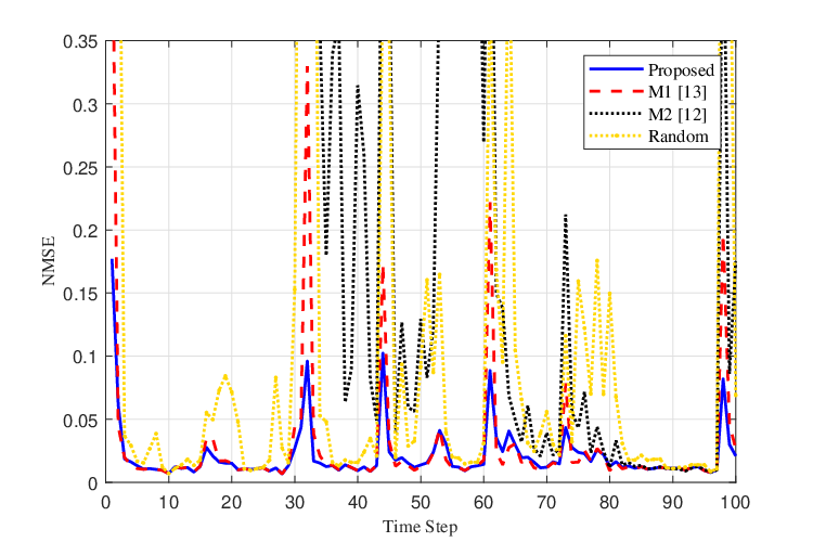
We first simulate the process of a heat source moving in a sensor network. The sensor network is modelled as a graph with 100 vertices randomly placed in a unit square and the edges exist between vertices of which the distance is no more than 0.6. The heat source moves in a given trajectory which is generated by a random walk. The evolution matrix of GS is given by the a graph translation [24] operator according to the trajectory. For example, if the center vertices of the trajectory for two continuous time steps are vertex $a$ and $b$, the evolution matrices will be $\tilde{H}_{t}=\text{diag}(\mathbf{V}^{\text{T}}\bm{\delta}_{a})$ and $\tilde{H}_{t+1}=\text{diag}(\mathbf{V}^{\text{T}}\bm{\delta}_{b})$. The energy of the GS at each time step is normalized to 1. The evolution and observation noise are i.i.d zero-mean Gaussian white noise with $\sigma_{\mathbf{v}}^{2}=10^{-4}$ and $\sigma_{\mathbf{w}}^{2}=10^{-3}$. The initialization states of the GS are $\hat{\mathbf{f}}_{0}^{+}=\mathbf{1}_{N\times 1}$ and $\mathbf{P}_{0}^{+}=\mathbf{I}_{N\times N}$. The discount factor $\gamma$ is set to $\gamma=0.8$. The average sampling budget $M=10$ and the largest budget of each time $M_{t}=20$. For the compared algorithms, the sampling budget of each time step is fixed to 10. The accumulated tracking error for 1000 time steps is shown in the second line of Table. 1. The step-by-step tracking performance of the first 100 time steps is shown in Fig. 1.

We can find that M1 and random sampling almost lose tracking of the GS and the proposed algorithm improves the tracking performance significantly compared to M2 when the signal evolution between two time steps is abrupt. A visualized demonstration of the abrupt heat source translation from time step 31 to 32 is shown in Fig. 2 (a) (b), the circled vertices are the sampled vertices among which the center vertex is in the full line circle and the others are in dashed line circles. It can be seen that since the long-term performance is considered, the proposed algorithm allocates more sampling budget to time step 32 to make the estimation at step 32 more accuracy.

Next, we show that our sampling policy also fits for the tracking of GS on time-varying topology, like RES graph. The opinion evolution in the social network is taken as an example. A community graph with 7 communities is used to model a social network. The probability that a edge $e=(i,j)$ in the edge set $\mathcal{E}$ is activated at time $t$ is set to $p_{i,j}=0.5$. The edges are activated independently across time. At each time step $t$, we draw a graph realization $\mathcal{G}_{t}=(\mathcal{V},\mathcal{E}_{t})$ from the underlying graph $\mathcal{G}=(\mathcal{V},\mathcal{E})$, where the edge set $\mathcal{E}_{t}\subseteq\mathcal{E}$ is generated via an i.i.d. Bernoulli process. An example of the RES community graph is shown in Fig. 3.

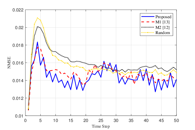
The opinion dynamics of individuals in the network follows the Krause-Hegselmann’s model [25], which consider the opinion evolution of the individuals as a weighted average of their opinions at a previous time with bounded confidence. The evolution of the GS on vertex $i$ at time step $t$ follows

where $I(i,\mathbf{f}_{t})=\left\{1\leq j\leq N|\,\left|(\mathbf{f}_{t})_{i}-(\mathbf{f}_{t})_{j}\right|\leq\epsilon\right\}$ and $|I(i,\mathbf{f}_{t})|$ denotes the cardinality of $I(i,\mathbf{f}_{t})$. The opinions of individuals are initialized by uniform random numbers in $[0,1]$ with $\mathbf{P}_{0}^{+}=0.1\mathbf{I}_{N\times N}$ and $\epsilon$ is set to 0.3. The energy of the GS at each time step is also normalized to 1. The evolution and observation noise are i.i.d. zero-mean Gaussion white noise with $\sigma_{\mathbf{v}}^{2}=10^{-4}$ and $\sigma_{\mathbf{w}}^{2}=10^{-4}$. The average sampling budget is set to $M=10$ and the largest budget of each time step is $M_{t}=20$, and the discount factor is set to $\gamma=0.8$. The accumulated tracking error for 100 time steps is shown in the third line of Table. 1, and the step-by-step tracking performance is shown in Fig. 4. In this case, the opinions on the social network become more and more smooth with time passing by according to (15), and therefore a more accurate estimation of GS in the former time step will help to estimate the GS in the later time step more accurately. By allocating more samples to the former time step, algorithm 1 also performance better in the long-term compared to the other methods with fixed sampling budget in each time step.

In this paper, a sampling policy with adaptive budget allocation is proposed for tracking a time-varying graph signal with KF. By considering the influence of the current sampling policy to the future performance, we formulate the problem as an infinite horizon sequential decision process. An approximate solution is obtained by truncating the future horizon to one, which improves the tracking performance a lot.

This work was supported by the Shanghai Municipal Natural Science Foundation (19ZR1404700), National Major Scientific Research Instruments and Equipments Development Project of NSFC (11827808), and Fudan-Zhuhai Innovation Institute.

Theorem 2: The object function in (3.2) is a convex function of the relaxed $(\tilde{\mathbf{D}}_{t},\tilde{\mathbf{D}}_{t+1})$.

References

- [1] B. Girault, “Stationary graph signals using an isometric graph translation,” in EUSIPCO. IEEE, 2015, pp. 1516–1520.
- [2] N. Perraudin and P. Vandergheynst, “Stationary signal processing on graphs.” IEEE Trans. Signal Process., vol. 65, no. 13, pp. 3462–3477, 2017.
- [3] A. Loukas and D. Foucard, “Frequency analysis of time-varying graph signals,” in GlobalSIP. IEEE, 2016, pp. 346–350.
- [4] E. Isufi, A. Loukas, A. Simonetto, and G. Leus, “Separable autoregressive moving average graph-temporal filters,” in EUSIPCO. IEEE, 2016, pp. 200–204.
- [5] A. W. Bohannon, B. M. Sadler, and R. V. Balan, “A filtering framework for time-varying graph signals,” in Vertex-Frequency Analysis of Graph Signals. Springer, 2019, pp. 341–376.
- [6] X. Mao and Y. Gu, “Time-varying graph signals reconstruction,” in Vertex-Frequency Analysis of Graph Signals. Springer, 2019, pp. 293–316.
- [7] Z. Wei, B. Li, and W. Guo, “Optimal sampling in joint time-and graph-domains for dynamic complex networks,” arXiv preprint arXiv:1901.11405, 2019.
- [8] A. Anis, A. Gadde, and A. Ortega, “Efficient sampling set selection for bandlimited graph signals using graph spectral proxies,” IEEE Trans. Signal Process., vol. 64, no. 14, pp. 3775–3789, 2016.
- [9] S. Chen, R. Varma, A. Sandryhaila, and J. Kovačević, “Discrete signal processing on graphs: Sampling theory,” IEEE Trans. Signal Process., vol. 63, no. 24, pp. 6510–6523, 2015.
- [10] X. Xie, H. Feng, J. Jia, and B. Hu, “Design of sampling set for bandlimited graph signal estimation,” GlobalSIP, pp. 653–657, Nov 2017.
- [11] P. Di Lorenzo, P. Banelli, E. Isufi, S. Barbarossa, and G. Leus, “Adaptive graph signal processing: Algorithms and optimal sampling strategies,” IEEE Trans. Signal Process., 2018.
- [12] E. Isufi, P. Banelli, P. Di Lorenzo, and G. Leus, “Observing and tracking bandlimited graph processes from sampled measurements,” Signal Process., vol. 177, pp. 1–13, 2020.
- [13] X. Shen and P. K. Varshney, “Sensor selection based on generalized information gain for target tracking in large sensor networks,” IEEE Trans. Signal Process., vol. 62, no. 2, pp. 363–375, 2014.
- [14] S. P. Chepuri and G. Leus, “Sparsity-promoting adaptive sensor selection for non-linear filtering.” in ICASSP, 2014, pp. 5080–5084.
- [15] E. Isufi, A. Loukas, A. Simonetto, and G. Leus, “Filtering random graph processes over random time-varying graphs,” IEEE Transactions on Signal Processing, vol. 65, no. 16, pp. 4406–4421, 2017.
- [16] A. Sandryhaila and J. M. Moura, “Discrete signal processing on graphs: Frequency analysis,” IEEE Trans. Signal Process., vol. 62, no. 12, pp. 3042–3054, 2014.
- [17] L. F. O. Chamon and A. Ribeiro, “Greedy sampling of graph signals,” IEEE Transactions on Signal Processing, vol. 66, no. 1, pp. 34–47, 2018.
- [18] A. Raj, A. Kuceyeski, and M. Weiner, “A network diffusion model of disease progression in dementia,” Neuron, vol. 73, no. 6, pp. 1204–1215, 2012.
- [19] Y. Wu, S. Liu, K. Yan, M. Liu, and F. Wu, “Opinionflow: Visual analysis of opinion diffusion on social media,” IEEE Trans. Vis. Comput. Graphics, vol. 20, no. 12, pp. 1763–1772, 2014.
- [20] D. P. Bertsekas, Dynamic programming and optimal control. Athena scientific Belmont, MA, 2005, vol. 1, no. 3.
- [21] A. massoud Farahmand, D. Nikovski, Y. Igarashi, and H. Konaka, “Truncated approximate dynamic programming with task-dependent terminal value,” in AAAI, 2016.
- [22] D. V. Djonin, Q. Zhao, and V. Krishnamurthy, “Optimality and complexity of opportunistic spectrum access: A truncated markov decision process formulation,” in 2007 IEEE International Conference on Communications, 2007, pp. 5787–5792.
- [23] S. Boyd and L. Vandenberghe, Convex optimization. Cambridge university press, 2004.
- [24] D. I. Shuman, S. K. Narang, P. Frossard, A. Ortega, and P. Vandergheynst, “The emerging field of signal processing on graphs: Extending high-dimensional data analysis to networks and other irregular domains,” IEEE Signal Process. Mag., vol. 30, no. 3, pp. 83–98, 2013.
- [25] R. Hegselmann and U. Krause, “Opinion dynamics and bounded confidence models, analysis and simulation,” Journal of Artificial Societies and Social Simulation, vol. 5, 07 2002.