Random telegraph signal analysis with a recurrent neural network
Abstract
We use an artificial neural network to analyze asymmetric noisy random telegraph signals (RTSs), and extract underlying transition rates. We demonstrate that a long short-term memory neural network can vastly outperform conventional methods, particularly for noisy signals. Our technique gives reliable results as the signal-to-noise ratio approaches one, and over a wide range of underlying transition rates. We apply our method to random telegraph signals generated by a superconducting double dot based photon detector, allowing us to extend our measurement of quasiparticle dynamics to new temperature regimes.
An asymmetric random telegraph signal is a signal which stochastic switches between two levels and . They are a common result of measurements on a wide variety of physical systems, including ion channels in cells Hille 2001, semiconductor devices such as transistors Kandiah 1994; Kandiah et al. 1989, quantum dots Efros and Rosen 1997 and optoelectronic devices Wang et al. 2006, high- superconductors Jung and Savo 1996, and single-Cooper-pair boxes Shaw et al. 2008, as well as being the building block of noise Kirton and Uren 1989. The transition rates from () to (), , are the accessible parameters describing the dynamics of the underlying system, and it is often desirable to extract them from the measured time sequence.
The most straightforward way to do this is to sample the time domain signal at some rate , divide it into periods in each of states and (Fig. 1(a)), histogram the dwell times and fit to the resulting distribution. However, the presence of noise and a finite measurement bandwidth will result in the measured statistics not representing the underlying system accurately. The problem is two-fold: noise whilst in one state can result in a false time period in the other state being detected (Fig. 1(b)), and a limited bandwidth means that genuine short-period excursions to the other state are not seen (Fig. 1(c)). This later effect also joins together the two time periods either side of the missed period, resulting in a false long period.
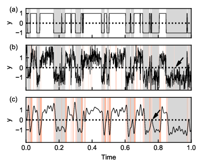
A variety of solutions to this problem have been proposed. Some focus on optimising the threshold at which the signal is divided into states 1 and 2 Yuzhelevski et al. 2000. Naaman and Aumentado modelled the detector as a separate process Naaman and Aumentado 2006a, and derived corrections to the measured rates. Other techniques include wavelet edge detection Prance et al. 2015, autocorrelation methods Martin-Martinez et al. 2014, cross corelation methods Küng et al. 2009, and analysis of the probability density function of the signal Lambert et al. 2017a; Singh et al. 2018.
In this Letter, we demonstrate that a recurrent neural network can be used to extract the underlying rates from noisy, bandwidth limited random telegraph signals. Neural networks (NNs) comprise an input layer holding the data to be analyzed, an output layer giving the result of the analysis, and one or more ‘hidden’ layers of any number of nodes. The connections between nodes can be arranged in a wide variety of different topologies, depending on the nature of the analysis to be performed. The weights of the internode connections are tuned using gradient descent methods to achieve the optimal mapping between the possible input vectors and the desired output vectors, a process referred to as ‘training’. Neural networks have proven to be a versatile tool, capable of tackling diverse problems including image recognition, financial fraud detection and natural language processing. They have also proven useful for the physical sciences, and have been applied to astrophysical images Banerji et al. 2010; Hezaveh et al. 2017, meta-analysis of the scientific literature Tshitoyan et al. 2019, the generation of quantum error correction algorithms Fösel et al. 2018, and the characterization of quantum dots Kalantre et al. 2019 and dopants Usman et al. 2019 in semiconductors.
Recurrent NNs are a class of NN which act sequentially in a particular direction along an input data array, with an internal memory allowing correlations between data points to affect the output. They are therefore particularly suitable for time sequence data. We use a long short-term memory (LSTM) Hochreiter and Schmidhuber 1997 architecture, a recurrent NN designed for time sequences in which related information can have significant temporal separation, such as speech Graves et al. 2013 and handwriting Graves et al. 2008 recognition, and musical analysis Eck and Schmidhuber 2002.
| Layer | Type | Size | Activation |
|---|---|---|---|
| Input | - | - | |
| 1 | LSTM | 128 | sigmoid |
| 2 | Fully connected | 128 | elu |
| 3 | Fully connected | 128 | elu |
| 4 | Fully connected | 128 | elu |
| 5 | Fully connected | 10 | elu |
| Output | - | 1 | relu |
Our NN has an input size of time samples, followed by an LSTM layer with internal size 128 (Table 1). The subsequent fully connected hidden layers are of sizes 128, 128, 128 and 10, with elu activation Clevert et al. 2015 functions. The output uses relu activation to ensure a non-negative output value, and is single valued; we exploit the symmetry of the RTS by training for only one rate, with the other accessible by simply inverting the signal, such that . This gives faster and more accurate training.
We implement the NN in Python 3.7 using Keras Chollet et al. 2015, with the Tensorflow back end. Training and prediction is accelerated by the use of a Nvidia Tesla K40c GPU. The NN was typically trained over 250 epochs, with 100 steps per epoch, taking around 13.6 hours. The NN is trained using synthetic RTSs, generated with independent rates and uniformly distributed on the interval between and . Rather than , we train for , to compress the output space.
We find that a realistic noise model is necessary for accurate analysis of real data. Two components of additive noise are generated: one with a power spectrum and randomized phase, representing, for example, noise processes in a semiconductor substrate; and one with a flat power spectrum and randomized phase, representing instrumentation noise. The amplitude of the noise added to the training data can be fixed to reflect the measured experimental noise, or varied over a wider distribution. We find that, in general, the NN cannot be successfully trained if presented with noisy data initially. Instead the training is started with noise free data, and the noise amplitude (or range of amplitudes) is increased every 20 training epochs until the desired level is reached. Finally, the generated signals are normalized such that they have mean 0 and standard deviation 1.

Once trained, the effectiveness of the NN can be tested by applying it to RTS data sequences. In Fig. 2 we compare the results of testing our NN on synthetic data of length samples to alternative methods. The NN is applied to RTSs with logarithmically spaced transition rates in the range , signal levels and noise with standard deviations 0 (no additive noise), 0.2, 0.4, and 0.6 (examples in upper panels). In Fig. 2 a-d we show the results of analysis of 100 RTSs for each rate pair by the time period histogram method (middle panels) and our NN (lower panels). The red dashed grid marks the underlying rates of the synthesised signals.
The NN is more effective for all noise levels. It is less accurate when one or both rates are low, and so there are fewer events to analyze, or equivalently the total power in the signal is low. Signals with higher rates and higher noises are also challenging, reflecting the similarity between a short period in a particular state and a spike due to noise. Nevertheless, the NN still performs well for regimes in which the time period histogram method fails completely, being particularly vulnerable to errors caused by noise.

In Fig. 3 we study the effect of filtering the RTS. The noise level for synthetic signals is now fixed at 0.4, and they are filtered using a 5th order digital Butterworth filter with cutoffs of , and , and again analyzed using appropriately trained NNs for each cutoff frequency. The NN is generally robust against low pass filtering when . If the rates are outside this regime, a significant spectral content of the signal is above the passband of the filter.
We now apply our neural network to RTSs due to microwave photon absorption processes in a superconducting double dot (SCDD) Lambert et al. 2014; Lambert et al. 2017b. The device comprises two aluminium superconducting islands coupled to each other by a Josephson junction, and to metallic leads by Superconducting-Insulator-Normal tunnel junctions (Fig. 4(a)). The charge state of the device is described by the differences in charge on each island from some arbitrarily chosen even charge state, and , and is labelled (, ). The behaviour of the device is governed by competition between the superconducting gap and the charging energy . When the device is protected from quasiparticle excitations and the charge residing on each island is quantised in units of .
The energy curvature associated with the anticrossing between the (0,2) and (2,0) charge states gives the device a finite quantum capacitance, but this can be removed by the destruction of coherence due to the presence of unpaired electrons, a process known as quasiparticle poisoning Naaman and Aumentado 2006b; Ferguson et al. 2006; Lutchyn et al. 2005. By monitoring the quantum capacitance of the SCDD via radiofrequency reflectrometry, Cooper pair breaking and reforming events can be observed. Time domain measurements (Fig. 4(d), upper panel) yield an RTS with one rate determined by the vulnerability of the Cooper pairs to incident photons, and the other determined by the recombination dynamics.

Because the transitions between charge configurations are driven by the energy difference between the states, it is interesting to study the transition rates as a function of temperature and applied magnetic field, which affect the state’s free energy via changes in entropy and the superconducting gap. For low temperatures () and magnetic fields (), rates can be determined by applying thresholding methods to the measured signal. But at higher temperatures and fields, the quality of the phase signal is sufficiently degraded (Fig. 4(d), lower panel) that this technique does not work.
Time traces with an acquisition time of and comprising phase measurements were taken at temperatures of , and , and at fields of . The demodulated phase signal was filtered with a cutoff of before sampling. For each field and temperature, measurements were made at points along a line in the charge stability diagram corresponding to transfer of charge from one island to the other, labelled in Fig. 4(b). Traces were found to have a low signal-to-noise ratio, with no obvious random telegraph behaviour (Fig. 4(d), lower panel). Rates can nevertheless be extracted using our NN. In Fig. 5 we plot the rates at zero detuning for increasing field at three temperatures, and observe the super-exponential behaviour previously seen at lower temperatures
To validate the rates extracted using our NN, we compare the mean phase for each measured trace with the expected mean value for an RTS having extracted rates and ,
| (1) |
In each case this is a measure of the excited state occupancy Esmail et al. 2017. In Fig. 5(b) we plot the measured mean signals (left) and deduced excited state occupancy (right). The agreement is excellent, demonstrating the efficacy of our NN for analysis of experimental data.

In summary, we find that an LSTM recurrent neural network is a powerful tool for the determination of the transition rates underlying noisy random telegraph signals with finite sampling rates. The network architecture is simple, yet versatile enough to apply to different signal parameters, and can be trained in a reasonable time on relatively modest hardware. This has allowed us to analyze previously inaccessible signals, and is particularly useful for measurement of delicate quantum systems for which measurements are difficult, and the SNR likely to be low.
We would like to acknowledge support from the MBIE (NZ) Endeavour Smart Ideas fund, Hitachi Cambridge Laboratory, and UK EPSRC Grant No. EP/K027018/1. A.J.F. was supported by a Hitachi Research fellowship.
References
- Hille (2001) B. Hille, Ion Channels of Excitable Membranes, third edition ed. (Sinauer Associates, Sunderland, Massachusetts, 2001).
- Kandiah (1994) K. Kandiah, IEEE Transactions on Electron Devices 41, 2006 (1994).
- Kandiah et al. (1989) K. Kandiah, M. O. Deighton, and F. B. Whiting, Journal of Applied Physics 66, 937 (1989).
- Efros and Rosen (1997) A. L. Efros and M. Rosen, Physical Review Letters 78, 1110 (1997).
- Wang et al. (2006) X. Wang, P. R. Rao, A. Mierop, and A. J. Theuwissen, in 2006 International Electron Devices Meeting (2006) pp. 1–4.
- Jung and Savo (1996) G. Jung and B. Savo, Journal of Applied Physics 80, 2939 (1996).
- Shaw et al. (2008) M. D. Shaw, R. M. Lutchyn, P. Delsing, and P. M. Echternach, Physical Review B 78, 024503 (2008).
- Kirton and Uren (1989) M. J. Kirton and M. J. Uren, Advances in Physics 38, 367 (1989).
- Yuzhelevski et al. (2000) Y. Yuzhelevski, M. Yuzhelevski, and G. Jung, Review of Scientific Instruments 71, 1681 (2000).
- Naaman and Aumentado (2006a) O. Naaman and J. Aumentado, Physical Review Letters 96, 100201 (2006a).
- Prance et al. (2015) J. R. Prance, B. J. V. Bael, C. B. Simmons, D. E. Savage, M. G. Lagally, M. Friesen, S. N. Coppersmith, and M. A. Eriksson, Nanotechnology 26, 215201 (2015).
- Martin-Martinez et al. (2014) J. Martin-Martinez, J. Diaz, R. Rodriguez, M. Nafria, and X. Aymerich, IEEE Electron Device Letters 35, 479 (2014).
- Küng et al. (2009) B. Küng, O. Pfäffli, S. Gustavsson, T. Ihn, K. Ensslin, M. Reinwald, and W. Wegscheider, Physical Review B 79, 035314 (2009).
- Lambert et al. (2017a) N. J. Lambert, A. A. Esmail, F. A. Pollock, M. Edwards, B. W. Lovett, and A. J. Ferguson, Physical Review B 95, 235413 (2017a).
- Singh et al. (2018) S. Singh, E. T. Mannila, D. S. Golubev, J. T. Peltonen, and J. P. Pekola, Applied Physics Letters 112, 243101 (2018).
- Banerji et al. (2010) M. Banerji, O. Lahav, C. J. Lintott, F. B. Abdalla, K. Schawinski, S. P. Bamford, D. Andreescu, P. Murray, M. J. Raddick, A. Slosar, A. Szalay, D. Thomas, and J. Vandenberg, Monthly Notices of the Royal Astronomical Society 406, 342 (2010).
- Hezaveh et al. (2017) Y. D. Hezaveh, L. P. Levasseur, and P. J. Marshall, Nature 548, 555 (2017).
- Tshitoyan et al. (2019) V. Tshitoyan, J. Dagdelen, L. Weston, A. Dunn, Z. Rong, O. Kononova, K. A. Persson, G. Ceder, and A. Jain, Nature 571, 95 (2019).
- Fösel et al. (2018) T. Fösel, P. Tighineanu, T. Weiss, and F. Marquardt, Physical Review X 8, 031084 (2018).
- Kalantre et al. (2019) S. S. Kalantre, J. P. Zwolak, S. Ragole, X. Wu, N. M. Zimmerman, M. D. Stewart, and J. M. Taylor, npj Quantum Information 5, 6 (2019).
- Usman et al. (2019) M. Usman, Y. Z. Wong, C. D. Hill, and L. C. L. Hollenberg, arXiv:1904.01756 [cond-mat, physics:physics, physics:quant-ph] (2019), arXiv:1904.01756 [cond-mat, physics:physics, physics:quant-ph] .
- Hochreiter and Schmidhuber (1997) S. Hochreiter and J. Schmidhuber, Neural computation 9, 1735 (1997).
- Graves et al. (2013) A. Graves, A.-r. Mohamed, and G. Hinton, in 2013 IEEE International Conference on Acoustics, Speech and Signal Processing (2013) pp. 6645–6649.
- Graves et al. (2008) A. Graves, M. Liwicki, H. Bunke, J. Schmidhuber, and S. Fernández, in Advances in Neural Information Processing Systems 20, edited by J. C. Platt, D. Koller, Y. Singer, and S. T. Roweis (Curran Associates, Inc., 2008) pp. 577–584.
- Eck and Schmidhuber (2002) D. Eck and J. Schmidhuber, in Artificial Neural Networks — ICANN 2002, Vol. 2415, edited by G. Goos, J. Hartmanis, J. van Leeuwen, and J. R. Dorronsoro (Springer Berlin Heidelberg, Berlin, Heidelberg, 2002) pp. 284–289.
- Clevert et al. (2015) D.-A. Clevert, T. Unterthiner, and S. Hochreiter, arXiv:1511.07289 [cs] (2015), arXiv:1511.07289 [cs] .
- Chollet et al. (2015) F. Chollet et al., https://keras.io (2015).
- Lambert et al. (2014) N. J. Lambert, M. Edwards, A. A. Esmail, F. A. Pollock, S. D. Barrett, B. W. Lovett, and A. J. Ferguson, Physical Review B 90, 140503(R) (2014).
- Lambert et al. (2017b) N. J. Lambert, A. A. Esmail, F. A. Pollock, M. Edwards, B. W. Lovett, and A. J. Ferguson, Physical Review B 95, 235413 (2017b).
- Naaman and Aumentado (2006b) O. Naaman and J. Aumentado, Physical Review B 73, 172504 (2006b).
- Ferguson et al. (2006) A. J. Ferguson, N. A. Court, F. E. Hudson, and R. G. Clark, Physical Review Letters 97, 106603 (2006).
- Lutchyn et al. (2005) R. Lutchyn, L. Glazman, and A. Larkin, Physical Review B 72, 014517 (2005).
- Esmail et al. (2017) A. A. Esmail, A. J. Ferguson, and N. J. Lambert, Applied Physics Letters 111, 252602 (2017).