On leptonic width of $X(4260)$

The $X(4260)$ resonance established by BABAR Collaboration in initial-state radiation (ISR) process $e^{+}e^{-}\rightarrow\gamma_{ISR}J/\psi\pi^{+}\pi^{-}$ in year 2005[1] (subsequently confirmed by CLEO[2] and Belle[3]), has attracted much attention since then. The mass and width of this resonance are given with $M=4230\pm 8$ MeV and $\Gamma=55\pm 19$ MeV [4], respectively, and $\Gamma_{ee}\times\mathrm{Br}(J/\psi\pi\pi)=9.7\pm 1.1$ eV [3] or $9.2\pm 1.5$ eV [5].

The property of $X(4260)$ becomes a very interesting topic since its discovery, because it is generally thought that there are not enough unassigned vector states in charmonium spectrum (taking into account the recently reported $X(4360)$, $X(4630)$/$X(4660)$ states), according to the naive quark model predictions [6]. The only such $1^{--}$ states expected up to $4.4$ GeV are generally $1S$, $2S$, $1D$, $3S$, $2D$ and $4S$, and they seem to be well established [7] – the situation is depicted in Figure 1.

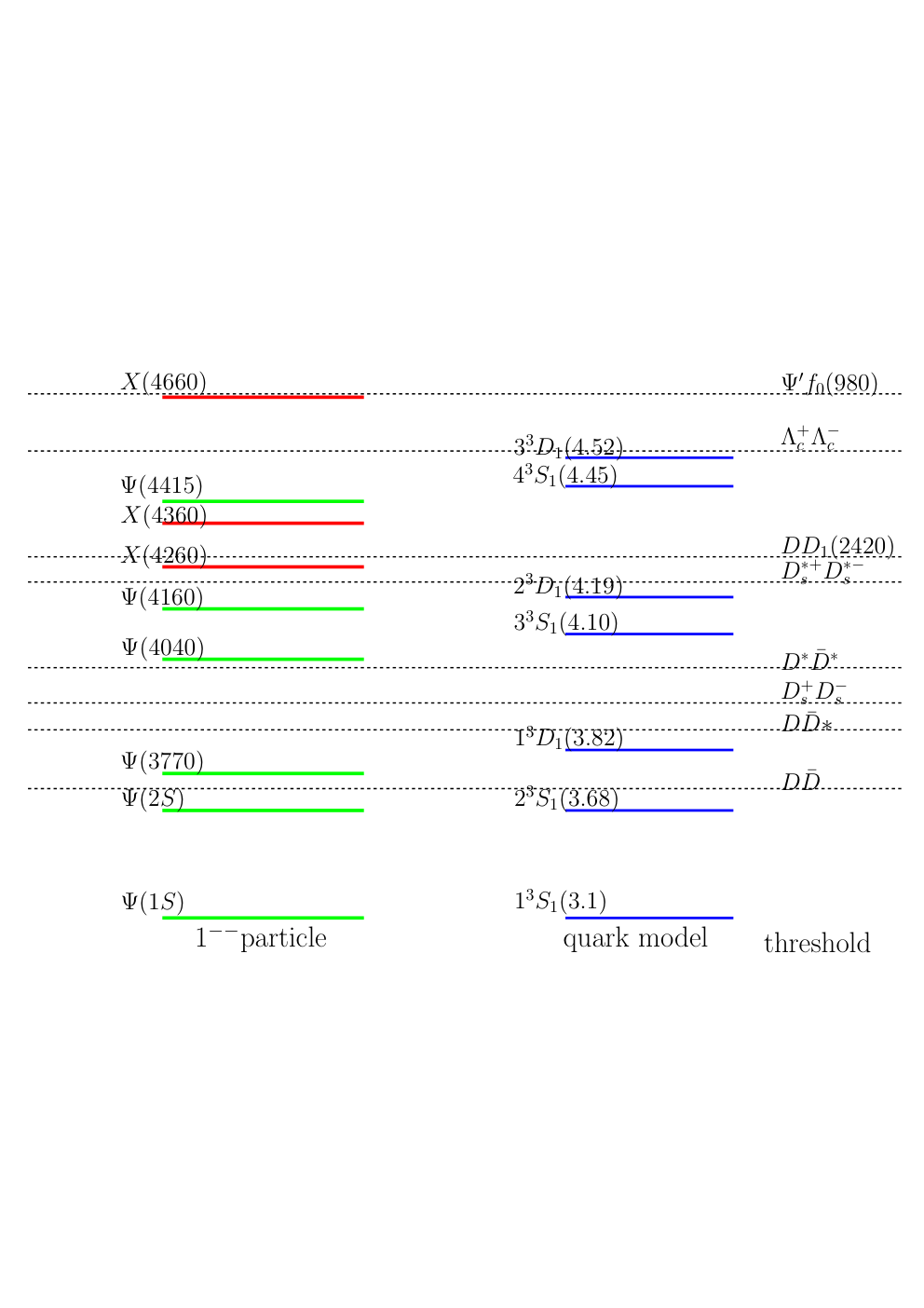
It is noticed that above $D\bar{D}$ threshold the number of $1^{--}$ states given by quark model prediction is inconsistent with that given by experiments. It is considered that the discrepancy between the naive quark model prediction and the observed spectrum is ascribed, at least partially, to the existence of many open charm thresholds, since the latter will distort the spectrum (see related discussions in, for example, Refs. [9, 8]). The situation is depicted in Figure 2.

Because of the situation as described above many studies have been devoted to the investigation of $X(4260)$.¹¹ 1 Here we apologize for only able to provide an incomplete list of references. The suggestions given by these studies may be classified into three types: hadronic molecule [10, 11, 12, 13, 14, 15]; $c\bar{c}$ state [16, 17, 18, 19, 20]; hybrid state [21, 22]; or non-resonant enhancement [23].

The open charm channels such as $D\bar{D},D\bar{D}^{*},D^{*}\bar{D}^{*}$ do not seem to be found in the final states of $X(4260)$ decays [26, 24, 25]. If this is indeed the case, then it would make $X(4260)$ even more mysterious, since the $J/\psi\pi\pi$ channel would become a very important, if not the dominant one. Hence the leptonic width $\Gamma_{e^{+}e^{-}}$ of $X(4260)$ would become very small, making it even harder to be understood as a conventional $1^{--}$ $\bar{c}c$ state, since the nearby $4^{3}S_{1}$ state is expected to have a leptonic width at the order $\sim 10^{3}$ eV [19].

In a previous publication, we have also studied the $X(4260)$ issue and suggested that there could be a sizable $\omega\chi_{c0}$ coupling [27], later confirmed by experimental researches [28]. At the same time, a very small $\Gamma_{e^{+}e^{-}}$ was found $\sim 25$eV. However, many new experimental results have appeared since then, measured by BESIII, Belle and BABAR experiments, such as $e^{+}e^{-}\to J/\psi\pi^{+}\pi^{-}$ [29, 5, 3], $h_{c}\pi^{+}\pi^{-}$ [30], $D^{0}D^{*-}\pi^{+}+c.c.$ [31], $\psi(2S)\pi^{+}\pi^{-}$ [32, 33, 34], $\omega\chi_{c0}$ [36, 35], $J/\psi\eta$ [37, 38] and $D_{s}^{*+}D_{s}^{*-}$ [39]. Hence the analyses of Ref. [27] urgently need to be upgraded. Among all it is worthwhile mentioning the $D_{s}^{*+}D_{s}^{*-}$ data near the $X(4260)$ region [39], which indicates a strong enhancement of events above the $D_{s}^{*+}D_{s}^{*-}$ threshold. If this is true, our analyses show that it decisively changes our previous understandings on $X(4260)$ resonance: It could probably be described by the conventional $4^{3}S_{1}$ state heavily renormalized by the $D_{s}^{*+}D_{s}^{*-}$ continuum (maybe a small mixing with the $3^{3}D_{1}$ state as well). If the $D_{s}^{*+}D_{s}^{*-}$ data are excluded from the fit, however, the final result on $\Gamma_{e^{+}e^{-}}$ can still be at least $\mathcal{O}(10^{2})$ eV, i.e., much larger comparing with that of Ref. [27], owing to other new data available as mentioned above. As a consequence, the $X(4260)$ resonance may still be considered as a mixture of $3^{3}D_{1}$ and $4^{3}S_{1}$ states, i.e., a conventional $\bar{c}c$ resonance.

The paper is organized as follows: This section 1 is the introduction. A detailed description of hadronic cross sections of $e^{+}e^{-}$ annihilation will be given in section 2. In section 3, combined fits to the hidden charm and open charm decay channels are performed, with two scenarios: one includes the $D_{s}^{*+}D_{s}^{*-}$ cross section data and the other does not. We leave physical discussions and conclusions in section 4.

To begin with, the $X(4260)$ propagator is written in the following form:

where $M_{X}$ represents the mass of $X(4260)$ and $\Gamma_{tot}(s)$ is the total momentum dependent width comprising of all partial ones: ²² 2 We do not consider a term $\propto\Gamma_{DD_{1}}$ here, as it is found vanishing in Ref. [27]. Also the experimental data in $Z_{c}\pi$ channel is absent. Since the $Z_{c}(3900)$ state is identified as a $DD^{*}$ molecule [40, 41], the experimental branching ratio is naturally expected to be small.

Considering the isospin symmetry, it is noticed that $\Gamma_{J/\psi\pi\pi}(s)=\frac{3}{2}\Gamma_{J/\psi\pi^{+}\pi^{-}}(s)$, $\Gamma_{h_{c}\pi\pi}(s)=\frac{3}{2}\Gamma_{h_{c}\pi^{+}\pi^{-}}(s)$, $\Gamma_{D\bar{D}^{*}\pi}(s)=3\Gamma_{D^{0}D^{*-}\pi^{+}+c.c.}(s)$, $\Gamma_{\psi(2S)\pi\pi}(s)=\frac{3}{2}\Gamma_{\psi(2S)\pi^{+}\pi^{-}}(s)$, $\Gamma_{D\bar{D}}=2\Gamma_{D^{+}D^{-}}$, $\Gamma_{D\bar{D}^{*}}=2\Gamma_{D^{+}D^{*-}+c.c.}$ and $\Gamma_{D^{*}\bar{D}^{*}}=2\Gamma_{D^{*+}D^{*-}}$. ³³ 3 Hereafter, the notation $D^{0}D^{*-}\pi^{+}$ and $D^{+}D^{*-}$ indicate $D^{0}D^{*-}\pi^{+}+c.c.$ and $D^{+}D^{*-}+c.c.$ for simplicity, respectively.

As for the $J/\psi\pi^{+}\pi^{-}$, $h_{c}\pi^{+}\pi^{-}$, $D^{0}D^{*-}\pi^{+}$ and $\psi(2S)\pi^{+}\pi^{-}$ channels, the three body partial decay width takes the standard form [4],⁴⁴ 4 Here we use the subscript “$f$” to represent various three body decay final states.

where $p_{ij}=p_{i}+p_{j}$, $m_{ij}^{2}=p_{ij}^{2}$, $|p_{1}^{*}|$, $\Omega_{1}^{*}$ are the momentum and angle of particle 1 in the rest frame of the system of particle 1 and 2, respectively; $\Omega_{3}$ is the angle of particle 3 in the rest frame of particle $M_{X}$; and $|p_{1}^{*}|$, $|p_{3}|$ are defined as

With respect to $J/\psi\pi^{+}\pi^{-}$ channel, the amplitude in Eq. (3) is calculated using the effective Lagrangian as Eq. (6) in Ref. [27] to describe the $X(4260)\to J/\psi\pi^{+}\pi^{-}$ process and the interaction coefficients $h_{i}(i=1,2,3)$ are listed in Tables 1 and 2. Since the production ratio $R=(\sigma(e^{+}e^{-}\to Z_{c}(4020)^{\mp}\pi^{\pm}\to h_{c}\pi^{+}\pi^{-})/\sigma(e^{+}e^{-}\to h_{c}\pi^{+}\pi^{-}))<20\%$ [42], $g_{h_{c}\pi^{+}\pi^{-}}$ can be used to describe the invariant amplitude in Eq. (3) when ignoring the resonance structure in the $X(4260)$ decay. Analogously, $g_{D^{0}D^{*-}\pi^{+}}$, $g_{\psi(2S)\pi^{+}\pi^{-}}$ can also be introduced as the invariant amplitude in Eq. (3) for $D^{0}D^{*-}\pi^{+}$ and $\psi(2S)\pi^{+}\pi^{-}$ channels for simplicity. Besides, in the analyses below, it is noticed that the decay ratios of these channels account for only a tiny share. Hence, it is feasible to employ $g_{h_{c}\pi^{+}\pi^{-}}$, $g_{D^{0}D^{*-}\pi^{+}}$ and $g_{\psi(2S)\pi^{+}\pi^{-}}$ for simplicity.

In addition, the two body decay widths take the following simple forms:

In above $k_{\omega\chi_{c0}}$, $k_{J/\psi\eta}$, $k_{D_{s}^{*+}D_{s}^{*-}}$, $k_{D^{+}D^{-}}$, $k_{D^{+}D^{*-}}$ and $k_{D^{*+}D^{*-}}$ are three momentums of $\omega\chi_{c0}$, $J/\psi\eta$, $D_{s}^{*+}D_{s}^{*-}$, $D^{+}D^{-}$, $D^{+}D^{*-}$ and $D^{*+}D^{*-}$ in $X(4260)$ rest frame, respectively. Further, except for the channels just discussed, there could be other channels with lower thresholds, for these channels we use a constant width $\Gamma_{0}$ to describe the overall effects.

Because the quantum number of $X(4260)$ is $J^{PC}=1^{--}$, the interaction between $X(4260)$ and photon can be written as

where $X_{\mu\nu}=\partial_{\mu}V_{\nu}-\partial_{\nu}V_{\mu}$ and $V^{\mu}$ represents the $X(4260)$ field, $F^{\mu\nu}=\partial^{\mu}A^{\nu}-\partial^{\nu}A^{\mu}$ describes the photon field. $g_{0}$ is the coefficient between the photon and $X(4260)$. So the decay width of $X(4260)\rightarrow e^{+}e^{-}$ reads

In $h_{c}\pi^{+}\pi^{-}$, $D^{0}D^{*-}\pi^{+}$, $\psi(2S)\pi^{+}\pi^{-}$, $\omega\chi_{c0}$, $J/\psi\eta$, $D_{s}^{*+}D_{s}^{*-}$, $D^{+}D^{*-}$ and $D^{*+}D^{*-}$ channels, using narrow width approximation, the cross section formulae take the form

where $k$ is the 3-momentum of incoming electron in $c.m.$ frame, $\Gamma_{ee}$ follows Eq. (8) and $\Gamma_{f}$ takes the form of Eq. (3) and Eq. (6). The term parameterized as a resonance propagator with a mass $M_{i}$ and width $\Gamma_{i}$ and the complex constant $\tilde{c}$ play the role of a background in each decay channel here, as will be declared in details in the forthcoming section 3.

In section 3.1, we will perform comprehensive fits to relevant data available in the vicinity of $X(4260)$, which include the $J/\psi\pi^{+}\pi^{-}$ [29, 5, 3], $h_{c}\pi^{+}\pi^{-}$ [30], $D^{0}D^{*-}\pi^{+}$ [31], $\psi(2S)\pi^{+}\pi^{-}$ [32, 33, 34], $\omega\chi_{c0}$ [36, 35], $J/\psi\eta$ [37, 38], $D_{s}^{*+}D_{s}^{*-}$ [39], together with the previous $D^{+}D^{*-}$ and $D^{*+}D^{*-}$ data in Ref. [25]. To be cautious, for the reason as already mentioned previously, the fit without $D_{s}^{*+}D_{s}^{*-}$ cross section data is also performed in section 3.2. Different results are carefully compared and discussed, and we believe that a clearer understanding on the nature of $X(4260)$ emerges.