Ground state phase diagram of dipolar-octupolar pyrochlores
Abstract
The “dipolar-octupolar” pyrochlore oxides R2M2O7 (R=Ce, Sm, Nd) represent an important opportunity in the search for three dimensional Quantum Spin Liquid (QSL) ground states. Their low energy physics is governed by an alluringly simple “XYZ” Hamiltonian, enabling theoretical description with only a small number of free parameters. Meanwhile, recent experiments on Ce pyrochlores strongly suggest QSL physics. Motivated by this, we present here a complete analysis of the ground state phase diagram of dipolar-octupolar pyrochlores. Combining cluster mean field theory, variational arguments and exact diagonalization we find multiple U(1) QSL phases which together occupy a large fraction of the parameter space. These results give a comprehensive picture of the ground state physics of an important class of QSL candidates and support the possibility of a QSL ground state in Ce2Zr2O7 and Ce2Sn2O7.
I Introduction
The pursuit of quantum spin liquid (QSL) ground states has not gone unrewarded. On the theory side, it has been realized that an enormous diversity of QSL states are possible Wen 2002; Savary and Balents 2017 and several physically relevant models are now known to have QSL ground states Kitaev 2006; Hermele et al. 2004; Banerjee et al. 2008; Gingras and McClarty 2014; Lee et al. 2014; Hu et al. 2015; Iqbal et al. 2016; Depenbrock et al. 2012; He et al. 2017. In experiment, many candidate materials have been established, exhibiting spin liquid like properties at low temperature Okamoto et al. 2007; Banerjee et al. 2016; Balz et al. 2016; Norman 2016; Sibille et al. 2018.
What has yet to be achieved is the combination of a material with an experimentally robust QSL state, with theoretical understanding of the microscopic interactions which give rise to that state and what kind of spin liquid they produce. Some materials studied as potential QSLs actually order at low temperature Chang et al. 2012; Cao et al. 2016; Takatsu et al. 2016, and others are complicated by chemical or structural disorder Kermarrec et al. 2014; Han et al. 2016; Martin et al. 2017; Zhu et al. 2017. Meanwhile, the relevant theoretical models are often complicated, possessing many free parameters Ross et al. 2011; Li et al. 2016; Essafi et al. 2017.
“Dipolar-octupolar” (DO) pyrochlores R2M2O7 (R=Ce, Sm, Nd; M=Zr, Hf, Ti, Sn, Pb) Sibille et al. 2015; Sibille et al. 2020; Gao et al. 2019; Gaudet et al. 2019; Peçanha-Antonio et al. 2019; Mauws et al. 2018; Singh et al. 2008; Malkin et al. 2010; Xu 2017; Lhotel et al. 2015; Xu et al. 2015; Petit et al. 2016; Xu et al. 2019; Anand et al. 2017; Bertin et al. 2015; Dalmas de Réotier et al. 2017; Hallas et al. 2015; Swarnakar et al. 2017 constitute an opportunity in this context, with their low energy physics being described by a simple XYZ Hamiltonian Huang et al. 2014; Rau and Gingras 2019. Out of this family, Ce2Sn2O7 Sibille et al. 2015; Sibille et al. 2020 and Ce2Zr2O7 Gao et al. 2019; Gaudet et al. 2019 have been highlighted recently as showing evidence of QSL physics. Notably, neutron scattering results for Ce2Zr2O7 bear encouraging similarity to predictions for a quantum spin liquid Gaudet et al. 2019; Benton et al. 2012.
In DO pyrochlores, the magnetic rare earth ions form a corner-sharing tetrahedral structure [Fig. 1 (inset)]. There are strong crystal electric fields (CEFs) acting on each magnetic site, resulting in a Kramers doublet at the bottom of the CEF spectrum, separated from higher states by a large gap Xu et al. 2015; Anand et al. 2017; Gaudet et al. 2019. With the scale of exchange interactions being Sibille et al. 2020; Xu et al. 2019, this motivates a description of the system in terms of pseudospin-1/2 operators . The thing which sets DO pyrochlores apart from other pyrochlore oxides is the transformation properties of these operators under time-reversal and lattice symmetries Huang et al. 2014; Rau and Gingras 2019. and both transform like the component of a magnetic dipole oriented along the site’s symmetry axis, while transforms like a component of the magnetic octupole tensor.
Assuming nearest-neighbor interactions, symmetry constrains the Hamiltonian to take the form Huang et al. 2014:
| (1) |
The final term in Eq. (1) can be removed by a suitably chosen global transformation Huang et al. 2014; Benton 2016, reducing the problem to an XYZ Hamiltonian:
| (2) |
An understanding of dipolar-octupolar pyrochlores and their potential to realize QSL ground states requires understanding of the ground state phase diagram of Eq. (2). Certain limits of the parameter space of Eq. (2) have been well studied, namely: the perturbative limit where one exchange parameter dominates the other two Hermele et al. 2004; Shannon et al. 2012; Benton et al. 2012, the XXZ limit where two of the three exchange parameters are equal Savary and Balents 2012; Lee et al. 2012; Benton et al. 2018; Banerjee et al. 2008; Kato and Onoda 2015; Huang et al. 2018a and the region of parameter space without a sign problem for Quantum Monte Carlo (QMC) Huang et al. 2014; Banerjee et al. 2008; Kato and Onoda 2015; Huang et al. 2018a; Huang et al. 2018b. However, there is no reason to expect materials of interest to fall into one of these limits, so a global phase diagram is needed.

In this Article, we calculate the ground state phase diagram of Eq. (2), by combining Cluster Mean Field Theory (CMFT), a variational extension to CMFT (CVAR) Benton et al. 2018 and Exact Diagonalization (ED). Where the results can be compared with available QMC results Huang et al. 2018b, they agree well. The final result for the phase diagram is shown in Fig. 1, with the parameter space expressed in terms of an overall scale which can be divided out and two angles :
| (3) |
We find four spin liquid phases, occupying a large combined portion of the parameter space, competing with an antiferromagnetic “all in/all out” (AIAO) phase and octupolar order. The four QSLs all host gapless photons and gapped fractionalized charges, and are thus realizations of emergent electromagnetism Hermele et al. 2004; Shannon et al. 2012; Benton et al. 2012; Gingras and McClarty 2014. They are labelled dipolar/octupolar- with the dipolar/octupolar label referring to whether the emergent electric field transforms like a magnetic dipole or octupole Li and Chen 2017; Yao et al. 2020, and the subscript referring to the flux penetrating elementary plaquettes in the ground state.
The remainder of this Article is devoted to explaining the calculations leading to Fig. 1, before finishing with a brief discussion of the outlook for experiments.
The Article is structured as follows:
- •
In Section II we describe some simple dualities which allow the whole phase diagram to be generated from calculations covering only a subregion of parameter space.
- •
In Section III we calculate the ground state phase diagram using CMFT, augmented with the CVAR approach.
- •
In Section IV we show ED calculations on a 16-site cluster, and use these as an alternative route to calculate the ground state phase diagram.
- •
- •
Section VI gives a summary of the results and an outlook for future work on dipolar-octupolar pyrochlores.
II Dualities of the model and reduced parameter space
In calculating the phase diagram it is useful to note that Eq. (2) has some dualities in which the exchange parameters can be permuted by a unitary transformation acting on . Specifically:
| (4) |
where represents a global rotation by an angle around axis of pseudospin space (which is not the same as a rotation in the physical crystal space). Making use of these dualities means that we do not actually need to study the full parameter space of , it is enough to consider a subset of parameters
| (5) |
from which we can then generate the rest of the phase diagram by applying the transformations from Eq. (4) to our results. The parameter space dsecribed by (5) is delineated by the black dashed lines in Fig. 1.

Taking to be the strongest exchange parameter as in (5), if it is clear that the ground state will simply order ferromagnetically with respect to the -axis of pseudospin space. In terms of the physical magnetic moments this implies AIAO order. The more challenging problem is to discover what happens when .
To study this case we rewrite the Hamiltonian in terms of spin ladder operators :
| (6) |
where and . The subregion of parameter space given by (5) then becomes:
| (7) |
III Phase diagram from Cluster Mean Field Theory
III.1 CMFT Calculation
To begin, we consider the phase diagram using a tetrahedral CMFT, as employed for the XXZ limit () in Ref. Benton et al. 2018. A summary of the calculation is given here, with a detailed description found in Appendix A.
To construct the CMFT we use the fact that the pyrochlore lattice can be divided into two sets of tetrahedra ‘A’ and ‘B’, with all neighbors of an ‘A’ tetrahedron being ‘B’ tetrahedra and vice versa. We then seek to optimize a product wave function over all ‘A’ tetrahedra:
| (8) |
The wave function on each tetrahedron is defined to be the ground state of a single tetrahedron Hamiltonian
| (9) |
contains the original exchange terms acting on the bonds of as well as auxiliary fields on each site
| (10) |
The auxiliary fields then serve as variational parameters for optimizing , and a CMFT wave function can be indexed by a configuration of on the lattice.
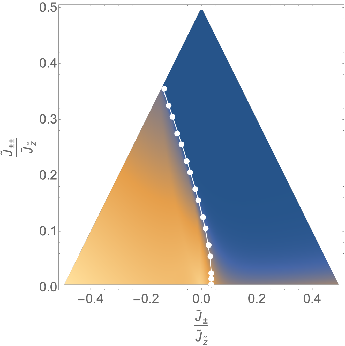
There are two regimes for the optimal configuration of in CMFT as shown in Fig. 2. For sufficiently large, positive, values of or the optimal solutions have ordered ferromagnetically along the -axis of pseudospin space. This implies , and therefore octupolar order since transforms like a magnetic octupole Huang et al. 2014.
In the remainder of the phase diagram there is a large, ice-like, degeneracy of disordered CMFT solutions, with where is a fixed, uniform, magnitude and , subject to the constraint that sum to zero on every tetrahedron.

III.2 Cluster variational (CVAR) calculation
To resolve the CMFT degeneracy in the disordered regime, we follow the cluster variational (CVAR) method Benton et al. 2018. The calculation is described briefly here with further details given in Appendix B.
Labelling CMFT ground states according to their configuration of signs we write down a generalized superposition of CMFT solutions
| (11) |
where are unknown coefficients. We then seek to optimize the new variational energy
| (12) |
Eq. (12) can be expanded in terms of the overlap between distinct CMFT wavefunctions, in a similar spirit to the derivation of dimer models from an expansion in the overlap between singlet coverings of a lattice Rokhsar and Kivelson 1988. This generates an effective Hamiltonian in the space of CMFT solutions, where the leading term is a six-site ring exchange which flips the values of on hexagonal plaquettes where alternates in sign around the plaquette, with matrix element .
This Hamiltonian has already been studied using Quantum Monte Carlo Shannon et al. 2012; Benton et al. 2012. It can have two different QSL ground states depending on the sign of . Both are U(1) QSLs with gapped, bosonic, charges and gapless photons. The two ground states are distinguished by the U(1) flux threading elementary plaquettes in the ground state. This background flux vanishes for (U(1)0) but is equal to on every plaquette for (U(1)π). The value of can be extracted from the CMFT calculation for all values of exchange parameters (see Appendix B), and by this means the degenerate region within CMFT can be divided into two ground state QSL phases (U(1)0 and U(1)π) depending on the sign of . The boundary between regions with different signs of is shown in Fig. 2. This constitutes our estimate of the boundary between 0-flux and -flux QSLs.
IV Exact Diagonalization

We now turn to ED calculations on a 16-site cubic cluster with periodic boundaries, to obtain alternative estimates of the phase boundaries.
IV.1 Boundary of octupolar ordered phase
Fig. 3(a) shows the second derivative of the ground state energy on this cluster with respect to , at various fixed values of . This second derivative exhibits a peak as is swept, indicating a qualitative change in the ground state Chaloupka et al. 2010.
Fig. 3(b), shows the position of these peaks as a function of and , laid over a color plot of the gap to excitations with odd total . The parity is conserved by , with the ground state always having . The line of peaks in the second derivative of the ground state energy coincides with a rapid decrease of the gap to excitations. This suggests the formation of a twofold degenerate ground state in the thermodynamic limit, breaking rotation symmetry around the axis, consistent with the octupolar order identified in CMFT. We thus interpret the peaks in the second derivative of the ground state energy as indicative of a transition to octupolar order.
IV.2 Boundary between QSLs
It is not easy to cleanly distinguish between the two QSL phase, QSL0 and QSLπ using ED on a small cluster. However, some insight into how to identify the phase boundary can be gained by considering how this transition occurs in the perturbative limit and in the CVAR approach.
From the perspective of both perturbation theory and CVAR, the transition from QSL0 to QSLπ occurs when the leading tunnelling matrix element, , between ice-like states changes sign. At the point where vanishes, tunnelling is restricted to higher order processes and will therefore be suppressed, leading to a near restoration of the degeneracy of ice-like states.
Returning to ED, this suggests that the transition from QSL0 to QSLπ will be accompanied by a simultaneous collapse of many excited states, in the sector with even total , to near zero energy. Such a collapse is indeed observed in the ED data, as shown in Fig. 4(a). The position of this collective minimum in the gaps within the even sector constitutes the ED estimate of the phase boundary between the two QSLs. The phase boundary thus obtained is compared with that from CVAR in Fig. 4(b), with the two estimates agreeing closely.
IV.3 Combining information from CMFT/CVAR and ED
Combining the information from CMFT/CVAR and ED gives the phase diagram shown in Fig. 5.
For the CMFT and ED estimates of the octupolar phase boundary agree closely. For the ED estimates a larger region of octupolar order (and hence a smaller QSL region) than does the CMFT approach.
For the model has no sign problem from the perspective of QMC, and in this regime we can compare with previous QMC studies. Several previous QMC studies of the case have observed the transition from QSL0 to the ordered phase as is increased Banerjee et al. 2008; Kato and Onoda 2015; Huang et al. 2018a; Huang et al. 2018b. A recent QMC study by Huang et al Huang et al. 2018b has studied the behavior of this phase boundary as a function of . Comparison with these results can be used to adjudicate between ED and CVAR where they disagree. The ED calculation gives closer agreement with the QMC results from [Huang et al. 2018b] than CMFT/CVAR does, and therefore we will take the ED calculation as our estimate of the boundary of the octupolar phase.
The estimates of the boundary between the two QSL phases agree closely between CVAR and ED, as shown in Fig. 4 (b). There is, however, some difference between the two estimates at larger negative values of . For the purpose of Fig. 5 we use the boundary from CVAR because it gives a more direct prediction of the transition between the two states in the thermodynamic limit, as opposed to the more indirect inference from the behavior of gaps in ED.
V Construction of complete phase diagram

The phase diagram in Fig. 5 can then be extended to the full parameter space using the duality relations [Eq. (4)].
In doing this, we must take into account how the duality transformations act on the ground states. For example, the octupolar ordered phase with becomes an AIAO phase when acted on by a transformation which swaps the -axis with the -axis or -axis. On the other hand, transformations which swap only the -axis and -axis, don’t change the classification of the ground state phase because and transform equivalently under point-group and time reversal symmetries.
Similar considerations allow us to distinguish four different kinds of U(1) QSL, generated from the two in the phase diagram of Fig. 5. In the 0-flux and -flux QSLs in Fig. 5 the emergent electric field of the QSL Hermele et al. 2004; Savary and Balents 2012 and therefore transforms like a magnetic dipole. If we act a transformation that swaps the -axis and -axes, then and transforms like an octupole. We should therefore not only distinguish U(1) QSLs by the flux but by the dipolar or octupolar character of the emergent electric field, giving four distinct QSLs on the complete phase diagram Li and Chen 2017; Yao et al. 2020.
VI Summary and Outlook
We have thus established a phase diagram for the generic, symmetry allowed, nearest neighbour exchange Hamiltonian describing dipolar-octupolar (DO) pyrochlores R2M2O7 (R=Ce, Sm, Nd). The picture we arrive at is an encouraging one for the realization of QSL states. There are four distinct U(1) QSLs on the phase diagram of the generic nearest neighbor model, and between them they occupy % of the available parameter space.
Amongst materials, Ce2Zr2O7 Gao et al. 2019; Gaudet et al. 2019, Ce2Sn2O7 Sibille et al. 2015; Sibille et al. 2020 and Sm2Zr2O7 Xu 2017 stand out as lacking low temperature order. The Ce pyrochlores in particular seem promising with recent neutron scattering results on Ce2Zr2O7 bearing similarity to predictions for emergent photons Gaudet et al. 2019. Low energy correlations in Ce2Sn2O7 seem to be dominantly octupolar in nature Sibille et al. 2020, which would be consistent with either of the two octupolar spin liquids on the phase diagram [Fig. 1].
It will be important to establish estimates of the exchange parameters of Ce2Zr2O7 and Ce2Sn2O7, combining information from inelastic neutron scattering with fits to thermodynamic data. Mean field calculations in [Sibille et al. 2020] give an initial estimate for Ce2Sn2O7 of , while setting and to zero, in the basis of Eq. (1). This would place Ce2Sn2O7 in the Octupolar- region of the phase diagram. It would be useful to refine this estimate with all parameters allowed to be finite, and using calculations beyond mean field theory.
If refined parameterisations place Ce2Zr2O7 and Ce2Sn2O7 within the QSL regimes of Fig. 1, then this will be a strong indication that they are indeed U(1) QSLs, and the parameterized model will provide a platform for further theoretical study. Understanding the effects of disorder of the crystal structure is also likely to be crucial, particularly in regard to the possible substitution of magnetic Ce3+ with non-magnetic Ce4+ Gaudet et al. 2019.
For those DO pyrochlores that are known to possess magnetic order at low temperature, the spin
liquid phases may also manifest at finite temperature, as suggested recently in Nd2Zr2O7 Xu et al. 2020.
In such cases it may even be possible to tune into the QSL phase using chemical
or physical pressure, giving another avenue to realize these exotic states of matter.
Note:
After completion of this work, the author became aware of a recent paper by Patri et al Patri et al. 2020 which also
presents calculations of the ground state phase diagram of DO pyrochlores.
Acknowledgements: The author acknowledges useful discussions with Andrea Bianchi, Jonathan Gaudet, Bruce Gaulin, Ludovic Jaubert, Bella Lake, Kate Ross, Nic Shannon, Romain Sibille, Rajiv Singh, Evan Smith, Jianhui Xu and Danielle Yahne. The author also thanks Paul McClarty for comments on the draft manuscript.
Appendix A CMFT solutions in the ice-like régime

The CMFT proceeds by optimizing variational wavefunctions of the form:
| (13) |
where the product is over all ‘A’ tetrahedra [Fig. 6], is the configuration of auxiliary fields defined on each site and the single tetrahedron wavefunctions depend only on the fields on sites belonging to tetrahedron . The auxiliary fields are variational parameters for optimizing the CMFT energy
| (14) |
The wave functions are taken to be eigenstates of a single tetrahedron Hamiltonian
| (15) | |||
| (16) |
is then:
| (17) |
where the final term in Eq. (17) sums over bonds belonging to ‘B’ tetrahedra and accounts for the interactions on those tetrahedra.
There is a large region of the phase diagram [Fig. 2 of main text] in which the optimal solutions for take the form:
| (18) |
Correspondingly, the expectation values of the spin components are:
| (19) |
with and being uniform across the system, and fixed by the energy optimization for a given parameter set.
With this form for the auxiliary fields, the mean field energy [Eq. (17)] becomes
| (20) |
Any arrangement of signs such that
| (21) |
gives rise to the same value of , as can be inferred from the symmetries of the original Hamiltonian. The remaining terms in Eq. (20) are also the same for all configurations obeying Eq. (21). Thus we have a large degeneracy of mean field solutions in this regime.

Each arrangement of signs obeying Eq. (21) defines a CMFT wavefunction [via Eqs. (13), (16) and (18)] which we will denote with . Explicitly, the form of single tetrahedron wave functions (denoted simply as ) relates to the configuration of signs on in the following way, written in the basis diagonalizing :
| (22) |
The parameters and can always be chosen to be real. This choice, combined with the choice to define the first term on the right hand side of each line of (22) to be positive, removes any phase ambiguity in the CMFT wavefunctions. and vary as a function of the exchange parameters and are plotted in Fig. 7.
Appendix B Details of CVAR calculation

The goal of the CVAR calculation is to resolve the degeneracy of the CMFT solutions by considering a new trial wavefunction which is a superposition of the CMFT solutions:
| (23) |
where are, a priori unknown, complex, coefficients.
We then seek to optimize the variational energy
| (24) |
where is a matrix containing the Hamiltonian matrix elements between different CMFT wavefunctions and contains the overlaps (the CMFT wavefunctions are not generally orthogonal to one another)
| (25) | |||
| (26) |
It is then useful to define a new matrix with vanishing diagonal elements:
| (27) |
such that
| (28) |
We then relate the vector of coefficients , to a new normalized vector via:
| (29) | |||
| (30) |
The variational energy is then
| (31) |
where
| (32) |
The optimal superposition of CMFT solitions is then given by the ground state of and Eq. (29).
We then expand in terms of two overlap parameters and , which can be defined from the wavefunctions in Eqs. (22):
| (33) | |||
| (34) |
These two quantities are treated as small parameters for the purposes of the expansion and indeed they are small through most of the relevant parameter space, as shown in Fig. 8.
To expand Eq. (32) we note that all the diagonal elements of are unity, and the leading off diagonal elements (coming from the process illustrated in Fig. 9) so we can write
| (35) |
The first two terms of the expansion of are then:
| (36) |
The leading elements in are (again, from the process in Fig. 9) and the leading elements in are and so we henceforth drop the second term.
We then need to evaluate the leading matrix elements in which connect configurations of which differ on a single hexagonal plaquette as shown in Fig. 9. The matrix element to a flip a hexagon is . The sign of determines whether the ground state should be a 0 or flux QSL, with
| (37) | |||
| (38) |
as may be inferred from prior quantum Monte Carlo studies of the six-site ring exchange Hamiltonian Shannon et al. 2012 and from a unitary transformation which relates the sign-problem free case () to the frustrated case () Hermele et al. 2004.

Quite generally the matrix element of between two CMFT wavefunctions can be written as
| (39) |
where the first sum is over ‘A’ tetrahedra and the second is over bonds belonging to ‘B’ tetrahedra. is the original exchange Hamiltonian on tetrahedron (distinct from in Eq. (15)) and
| (40) |

The contribution of any ‘A’ tetrahedron which does not change configurations between and to Eq. (39) vanishes. Similarly, the contribution of any ‘B’ bond connecting two unchanged ‘A’ tetrahedra vanishes.
There are three kinds of non-vanishing contribution to the matrix element to flip a hexagon. Firstly, the three ‘A’ tetrahedra belonging to the flipped hexagon (highlighted in red in Fig. 10) contribute:
| (41) |
where
Secondly, there are contributions from ‘B’ bonds connecting to the interior of the flipped hexagon (highlighted in blue in Fig. 10):
| (43) |
Finally, there are contributions from ‘B’ bonds connecting to the exterior of the ‘A’ tetrahedra on the flipped hexagon (highlighted in green in Fig. 10):
| (44) |
where
Summing these contributions and accounting for the fact that must alternate around the hexagon and must obey Eq. (21) everywhere, we arrive at the matrix element:
| (46) |
References
- Wen (2002) X.-G. Wen, Phys. Rev. B 65, 165113 (2002).
- Savary and Balents (2017) L. Savary and L. Balents, Reports on Progress in Physics 80, 016502 (2017).
- Kitaev (2006) A. Kitaev, Annals of Physics 321, 2 (2006).
- Hermele et al. (2004) M. Hermele, M. P. A. Fisher, and L. Balents, Phys. Rev. B 69, 064404 (2004).
- Banerjee et al. (2008) A. Banerjee, S. V. Isakov, K. Damle, and Y. B. Kim, Phys. Rev. Lett. 100, 047208 (2008).
- Gingras and McClarty (2014) M. J. P. Gingras and P. A. McClarty, Reports on Progress in Physics 77, 056501 (2014).
- Lee et al. (2014) E. K.-H. Lee, R. Schaffer, S. Bhattacharjee, and Y. B. Kim, Phys. Rev. B 89, 045117 (2014).
- Hu et al. (2015) W.-J. Hu, S.-S. Gong, W. Zhu, and D. N. Sheng, Phys. Rev. B 92, 140403(R) (2015).
- Iqbal et al. (2016) Y. Iqbal, W.-J. Hu, R. Thomale, D. Poilblanc, and F. Becca, Phys. Rev. B 93, 144411 (2016).
- Depenbrock et al. (2012) S. Depenbrock, I. P. McCulloch, and U. Schollwöck, Phys. Rev. Lett. 109, 067201 (2012).
- He et al. (2017) Y.-C. He, M. P. Zaletel, M. Oshikawa, and F. Pollmann, Phys. Rev. X 7, 031020 (2017).
- Okamoto et al. (2007) Y. Okamoto, M. Nohara, H. Aruga-Katori, and H. Takagi, Phys. Rev. Lett. 99, 137207 (2007).
- Banerjee et al. (2016) A. Banerjee, C. A. Bridges, J.-Q. Yan, A. A. Aczel, L. Li, M. B. Stone, G. E. Granroth, M. D. Lumsden, Y. Yiu, J. Knolle, S. Bhattacharjee, D. L. Kovrizhin, R. Moessner, D. A. Tennant, D. G. Mandrus, and S. E. Nagler, Nature Materials 15, 733 (2016).
- Balz et al. (2016) C. Balz, B. Lake, J. Reuther, H. Luetkens, R. Schonemann, T. Herrmannsdorfer, Y. Singh, A. T. M. Nazmul Islam, E. M. Wheeler, J. A. Rodriguez-Rivera, T. Guidi, G. G. Simeoni, C. Baines, and H. Ryll, Nat. Phys. 12, 942 (2016).
- Norman (2016) M. R. Norman, Rev. Mod. Phys. 88, 041002 (2016).
- Sibille et al. (2018) R. Sibille, N. Gauthier, H. Yan, M. Ciomaga Hatnean, J. Ollivier, B. Winn, U. Filges, G. Balakrishnan, M. Kenzelmann, N. Shannon, and T. Fennell, Nature Physics 14, 711 (2018).
- Chang et al. (2012) L.-J. Chang, S. Onoda, Y. Su, Y.-J. Kao, K.-D. Tsuei, Y. Yasui, K. Kakurai, and M. R. Lees, Nature Communications 3, 992 (2012).
- Cao et al. (2016) H. B. Cao, A. Banerjee, J.-Q. Yan, C. A. Bridges, M. D. Lumsden, D. G. Mandrus, D. A. Tennant, B. C. Chakoumakos, and S. E. Nagler, Phys. Rev. B 93, 134423 (2016).
- Takatsu et al. (2016) H. Takatsu, S. Onoda, S. Kittaka, A. Kasahara, Y. Kono, T. Sakakibara, Y. Kato, B. Fåk, J. Ollivier, J. W. Lynn, T. Taniguchi, M. Wakita, and H. Kadowaki, Phys. Rev. Lett. 116, 217201 (2016).
- Kermarrec et al. (2014) E. Kermarrec, A. Zorko, F. Bert, R. H. Colman, B. Koteswararao, F. Bouquet, P. Bonville, A. Hillier, A. Amato, J. van Tol, A. Ozarowski, A. S. Wills, and P. Mendels, Phys. Rev. B 90, 205103 (2014).
- Han et al. (2016) T.-H. Han, M. R. Norman, J.-J. Wen, J. A. Rodriguez-Rivera, J. S. Helton, C. Broholm, and Y. S. Lee, Phys. Rev. B 94, 060409(R) (2016).
- Martin et al. (2017) N. Martin, P. Bonville, E. Lhotel, S. Guitteny, A. Wildes, C. Decorse, M. Ciomaga Hatnean, G. Balakrishnan, I. Mirebeau, and S. Petit, Phys. Rev. X 7, 041028 (2017).
- Zhu et al. (2017) Z. Zhu, P. A. Maksimov, S. R. White, and A. L. Chernyshev, Phys. Rev. Lett. 119, 157201 (2017).
- Ross et al. (2011) K. A. Ross, L. Savary, B. D. Gaulin, and L. Balents, Phys. Rev. X 1, 021002 (2011).
- Li et al. (2016) Y.-D. Li, X. Wang, and G. Chen, Phys. Rev. B 94, 035107 (2016).
- Essafi et al. (2017) K. Essafi, O. Benton, and L. D. C. Jaubert, Phys. Rev. B 96, 205126 (2017).
- Sibille et al. (2015) R. Sibille, E. Lhotel, V. Pomjakushin, C. Baines, T. Fennell, and M. Kenzelmann, Phys. Rev. Lett. 115, 097202 (2015).
- Sibille et al. (2020) R. Sibille, N. Gauthier, E. Lhotel, V. Porée, V. Pomjakushin, R. A. Ewings, T. G. Perring, J. Ollivier, A. Wildes, C. Ritter, T. C. Hansen, D. A. Keen, G. J. Nilsen, L. Keller, S. Petit, and T. Fennell, Nat. Phys. 16, 546 (2020).
- Gao et al. (2019) B. Gao, T. Chen, D. W. Tam, C.-L. Huang, K. Sasmal, D. T. Adroja, F. Ye, H. Cao, G. Sala, M. B. Stone, C. Baines, J. A. T. Verezhak, H. Hu, J.-H. Chung, X. Xu, S.-W. Cheong, M. Nallaiyan, S. Spagna, M. B. Maple, A. H. Nevidomskyy, E. Morosan, G. Chen, and P. Dai, Nature Physics 15, 1052 (2019).
- Gaudet et al. (2019) J. Gaudet, E. M. Smith, J. Dudemaine, J. Beare, C. R. C. Buhariwalla, N. P. Butch, M. B. Stone, A. I. Kolesnikov, G. Xu, D. R. Yahne, K. A. Ross, C. A. Marjerrison, J. D. Garrett, G. M. Luke, A. D. Bianchi, and B. D. Gaulin, Phys. Rev. Lett. 122, 187201 (2019).
- Peçanha-Antonio et al. (2019) V. Peçanha-Antonio, E. Feng, X. Sun, D. Adroja, H. C. Walker, A. S. Gibbs, F. Orlandi, Y. Su, and T. Brückel, Phys. Rev. B 99, 134415 (2019).
- Mauws et al. (2018) C. Mauws, A. M. Hallas, G. Sala, A. A. Aczel, P. M. Sarte, J. Gaudet, D. Ziat, J. A. Quilliam, J. A. Lussier, M. Bieringer, H. D. Zhou, A. Wildes, M. B. Stone, D. Abernathy, G. M. Luke, B. D. Gaulin, and C. R. Wiebe, Phys. Rev. B 98, 100401(R) (2018).
- Singh et al. (2008) S. Singh, S. Saha, S. K. Dhar, R. Suryanarayanan, A. K. Sood, and A. Revcolevschi, Phys. Rev. B 77, 054408 (2008).
- Malkin et al. (2010) B. Z. Malkin, T. T. A. Lummen, P. H. M. van Loosdrecht, G. Dhalenne, and A. R. Zakirov, Journal of Physics: Condensed Matter 22, 276003 (2010).
- Xu (2017) J. Xu, Magnetic Properties of Rare-Earth Zirconate Pyrochlores, Ph.D. thesis, Technischen Universität Berlin (2017).
- Lhotel et al. (2015) E. Lhotel, S. Petit, S. Guitteny, O. Florea, M. Ciomaga Hatnean, C. Colin, E. Ressouche, M. R. Lees, and G. Balakrishnan, Phys. Rev. Lett. 115, 197202 (2015).
- Xu et al. (2015) J. Xu, V. K. Anand, A. K. Bera, M. Frontzek, D. L. Abernathy, N. Casati, K. Siemensmeyer, and B. Lake, Phys. Rev. B 92, 224430 (2015).
- Petit et al. (2016) S. Petit, E. Lhotel, B. Canals, M. Ciomaga Hatnean, J. Ollivier, H. Mutka, E. Ressouche, A. R. Wildes, M. R. Lees, and G. Balakrishnan, Nature Physics 12, 746 (2016).
- Xu et al. (2019) J. Xu, O. Benton, V. K. Anand, A. T. M. N. Islam, T. Guidi, G. Ehlers, E. Feng, Y. Su, A. Sakai, P. Gegenwart, and B. Lake, Phys. Rev. B 99, 144420 (2019).
- Anand et al. (2017) V. K. Anand, D. L. Abernathy, D. T. Adroja, A. D. Hillier, P. K. Biswas, and B. Lake, Phys. Rev. B 95, 224420 (2017).
- Bertin et al. (2015) A. Bertin, P. Dalmas de Réotier, B. Fåk, C. Marin, A. Yaouanc, A. Forget, D. Sheptyakov, B. Frick, C. Ritter, A. Amato, C. Baines, and P. J. C. King, Phys. Rev. B 92, 144423 (2015).
- Dalmas de Réotier et al. (2017) P. Dalmas de Réotier, A. Yaouanc, A. Maisuradze, A. Bertin, P. J. Baker, A. D. Hillier, and A. Forget, Phys. Rev. B 95, 134420 (2017).
- Hallas et al. (2015) A. M. Hallas, A. M. Arevalo-Lopez, A. Z. Sharma, T. Munsie, J. P. Attfield, C. R. Wiebe, and G. M. Luke, Phys. Rev. B 91, 104417 (2015).
- Swarnakar et al. (2017) D. Swarnakar, Y. Jana, J. Alam, and S. Nandi, Physica B: Condensed Matter 521, 93 (2017).
- Huang et al. (2014) Y.-P. Huang, G. Chen, and M. Hermele, Phys. Rev. Lett. 112, 167203 (2014).
- Rau and Gingras (2019) J. G. Rau and M. J. Gingras, Annual Review of Condensed Matter Physics 10, 357 (2019).
- Benton et al. (2012) O. Benton, O. Sikora, and N. Shannon, Phys. Rev. B 86, 075154 (2012).
- Benton (2016) O. Benton, Phys. Rev. B 94, 104430 (2016).
- Shannon et al. (2012) N. Shannon, O. Sikora, F. Pollmann, K. Penc, and P. Fulde, Phys. Rev. Lett. 108, 067204 (2012).
- Savary and Balents (2012) L. Savary and L. Balents, Phys. Rev. Lett. 108, 037202 (2012).
- Lee et al. (2012) S.-B. Lee, S. Onoda, and L. Balents, Phys. Rev. B 86, 104412 (2012).
- Benton et al. (2018) O. Benton, L. D. C. Jaubert, R. R. P. Singh, J. Oitmaa, and N. Shannon, Phys. Rev. Lett. 121, 067201 (2018).
- Kato and Onoda (2015) Y. Kato and S. Onoda, Phys. Rev. Lett. 115, 077202 (2015).
- Huang et al. (2018a) C.-J. Huang, Y. Deng, Y. Wan, and Z. Y. Meng, Phys. Rev. Lett. 120, 167202 (2018a).
- Huang et al. (2018b) C.-J. Huang, C. Liu, Z.-Y. Meng, Y. Yue, Y. Deng, and G. Chen, arXiv:1806.04014 (2018b).
- Li and Chen (2017) Y.-D. Li and G. Chen, Phys. Rev. B 95, 041106(R) (2017).
- Yao et al. (2020) X. P. Yao, Y.-D. Li, and G. Chen, Phys. Rev. Research 2, 013334 (2020).
- Chaloupka et al. (2010) J. Chaloupka, G. Jackeli, and G. Khaliullin, Phys. Rev. Lett. 105, 027204 (2010).
- Rokhsar and Kivelson (1988) D. S. Rokhsar and S. A. Kivelson, Phys. Rev. Lett. 61, 2376 (1988).
- (60) Supplemental Material .
- Xu et al. (2020) J. Xu, O. Benton, A. T. M. N. Islam, T. Guidi, G. Ehlers, and B. Lake, Phys. Rev. Lett. 124, 097203 (2020).
- Patri et al. (2020) A. S. Patri, M. Hosoi, and Y. B. Kim, Phys. Rev. Research 2, 023253 (2020).