Geodesic motion around a supersymmetric AdS5 black holeJournal: Eur. Phys. J. C
Abstract
In this article the geodesic motion of test particles in the spacetime of a supersymmetric AdS5 black hole is studied. The equations of motion are derived and solved in terms of the Weierstrass , , and functions. Effective potentials and parametric diagrams are used to analyze and characterize timelike, lightlike, and spacelike particle motion and a list of possible orbit types is given. Furthermore, various plots of orbits are presented.
1 Introduction
The famous anti-de Sitter/conformal field theory (AdS/CFT) correspondence provides a relation between gravity and quantum field theory, in particular, Maldacena Maldacena:1997re connected compactifications of string theory on anti-de Sitter to a conformal field theory. Therefore, black holes that are asymptotically anti-de Sitter are very interesting to study.
A few years after Kerr Kerr:1963ud presented an asymptotically flat rotating black hole, Carter Carter:1968ks came up with the first rotating asymptotically anti-de Sitter black hole. In five dimensions Hawking et al. Hawking:1998kw found an AdS black hole with two rotation parameters. Five dimensional AdS black holes are especially interesting since the AdS5/CFT4 correspondence is very well understood and CFT can be described as SU(N) super Yang-Mills theory. One of the first supersymmetric AdS5 black hole solutions were found by Gutowski and Reall Gutowski:2004ez. They considered the minimal gauged supergravity theory described in Gauntlett:2003wb and found an asymptotically AdS5 black hole parameterized by its mass, charge, and two equal angular momenta. Many more black hole solutions in supergravity theories were found, see, e.g., Cvetic:2005zi.
The motion of test particles is a useful tool to study black holes in various theories of gravity. The solutions of the equations of motion can be applied to calculate observable quantities like the shadow of a black hole or the periastron shift of a bound orbit. Geodesics also provide information on the structure of a spacetime. In the framework of AdS/CFT, geodesics correspond to two-point correlators Balasubramanian:1999zv. In particular, spacelike geodesics with both endpoints on the boundary (i.e., escape orbits of particles with imaginary rest mass) are related to the eikonal approximation of holographic two-point functions. CFT correlators describe observables on the AdS boundary.
The Hamilton-Jacobi formalism represents an efficient method to derive the equations of motion for test particles. In the four-dimensional Kerr spacetime, Carter Carter:1968ks showed that the Hamilton-Jacobi equation for test particles separates. The resulting equations of motion can be solved analytically in terms of elliptic functions. In higher dimensions, or in spacetimes with a cosmological constant, the analytical solutions of the geodesic equations often require hyperelliptic functions Kraniotis:2005zm; Kraniotis:2006ux; Fujita:2009bp; Hackmann:2009nh; Hackmann:2010zz; Grunau:2017uzf. The geodesics in a rotating supersymmetric black hole spacetime were analyzed in Gibbons:1999uv; Diemer:2013fza, where the complete analytical solution of the geodesics equations in the supersymmetric Breckenridge-Myers-Peet-Vafa (BMPV) Breckenridge:1996is spacetime was presented. Here we will study the geodesic motion of test particles around the supersymmetric, asymptotically AdS5 black hole of Gutowski and Reall Gutowski:2004ez.
The article is structured as follows. We derive the equations of motion in Section 2 and give a complete classification of the geodesics in Section 3. In Section 4 we solve the equations of motion analytically in terms of the Weierstrass , , and functions. Finally we present some example plots of the orbits in Section 5 and conclude in Section 6.
2 The supersymmetric AdS5 black hole
Gutowski and Reall Gutowski:2004ez found a one-parameter family of supersymmetric AdS5 black holes. The metric is given by
| (1) |
where the can be expressed in terms of the Euler angles as
| (2a) | ||||
| (2b) | ||||
| (2c) | ||||
and the metric functions are
| (3) | ||||
| (4) | ||||
| (5) | ||||
| (6) |
The Maxwell potential is
| (7) |
Here is the radial coordinate of the black hole’s degenerate horizon, is the sign of its angular momentum, and is the AdS radius. Note that can be absorbed into , consequently, in the following analysis of the geodesics we set but examine the geodesic motion for arbitrary sign of .
It can be shown that the solution is asymptotically AdS5, by using the coordinate transformation , see Gutowski:2004ez. It has the Einstein universe as its conformal boundary and the has the radius . Boundary as well as bulk time translations are generated by . However, as for all rotating AdS black holes, there is another timelike Killing vector field in the bulk
| (8) |
If is used to generate time translations, we are working in a co-rotating frame and there is no ergoregion. If, on the other hand, generates time translations, then an ergoregion exists.
The metric (1) is characterized by its conserved quantities associated with symmetries of the conformal boundary, which was shown for asymptotically AdS spacetimes of dimension by Ashtekar and Das Ashtekar:1999jx. In this case, the black hole’s conserved quantities can be defined by an Ashtekar and Das mass
| (9) |
an angular momentum with respect to of
| (10) |
a vanishing angular momentum with respect to , an energy of
| (11) |
and a charge of
| (12) |
We then obtain
| (13) |
and therefore the solution saturates the BPS bound, see also Gutowski:2004ez. Note that the conserved charges by Ashtekar and Das are only correct for a special class of solutions, where the non-normalizable modes of all matter fields vanish and the Ricci curvature of the boundary metric also vanishes, unless . In Papadimitriou:2005ii the authors present well defined conserved charges for general asymptotically AdS black holes in the presence of matter.
The solution (1) has a smooth event horizon at and the spatial geometry of the horizon is a squashed
| (14) |
where the are defined as the with instead of . Behind the event horizon there is a curvature singularity at surrounded by a region of closed timelike curves Gutowski:2004ez.
2.1 The equations of motion
We use the Hamilton-Jacobi formalism to obtain the equations of motion for test particles in the spacetime of a supersymmetric black hole. To solve the Hamilton-Jacobi equation of an uncharged particle
| (15) |
we make the ansatz for the action
| (16) |
Here is the particle’s conserved energy, and are its conserved angular momenta along and , respectively, is an affine parameter along the geodesic, and is equal to 0 for light, equal to 1 for particles of positive mass, and equal to for particles of imaginary mass. The case corresponds to spacelike geodesics and is of relevance for AdS/CFT if the geodesics’ endpoints are on the boundary . This is discussed in more detail in Section 3.4.
Using this ansatz and the metric (1), the Hamilton-Jacobi equation (15) becomes
| (17) |
One can separate the Hamilton-Jacobi equation (15) by terms in and in
| (18) |
and
| (19) |
Here we introduced as a separation constant known as the Carter Carter:1968rr constant. Now we can solve Eq. (18) for and Eq. (19) for , which can then be used to substitute the functions and in the ansatz (16) (no need to actually compute the integrals here). Finally, the equations of motion can be deduced with a variational method; the derivatives of the action with respect to the constants of motion can be set to zero.
With the help of the Mino Mino:2003yg time given by to remove the factor from all equations and the substitution , this yields five differential equations of motion
| (20) |
| (21) |
| (22) |
| (23) |
| (24) |
The polynomial P and the function are
| (25) |
| (26) |
To simplify the equations of motion, dimensionless quantities were introduced by scaling with
| (27) | ||||||||||
This was achieved by setting and canceling factors of 4 in front of , , and for convenience.
3 Classification of the geodesics
The properties of the geodesics are determined by the polynomial P in Eq. (25) and the function in Eq. (26). The characteristics of and P are given by the particle’s constants of motion (energy, angular momenta, Carter constant, parameter) and the metric’s (positive or negative) AdS radius. In this section, features of the function and the polynomial P – and therefore the types of orbits – for various sets of constants of motion are studied. This is done analogously to Grunau:2010gd, where geodesic motion of electrically and magnetically charged test particles in the Reissner-Nordström spacetime has been examined.
3.1 The motion
To obtain real values of , the requirement has to be met. From this it follows that . The substitution turns Eq. (21) into
| (28) |
where , , and . Since holds, it follows . The zeros of the second degree polynomial correspond to angles that confine the particle’s motion. Note that for vanishing in Eqs. (21) and (23) the test particle’s motion is planar in the 3-dimensional subspace given by the spherical coordinates as in the Schwarzschild case.
The polynomial’s discriminant is given by and can be expressed as with . describes a downward opened parabola with zeros
| (29) |
and maximum at . A real solution implies real zeros of and thus requires . While is sufficient, other cases require an upper limit of given by . For symmetric motion with respect to the equatorial plane or have to vanish. Other cases are depending on the sign of :
- 1.
: The zeros of are either both positive or both negative, which confines the particle’s motion to for and for .
- 2.
: The zeros of are with for and for . With the additional condition , the orbit fills an entire hemisphere [see Fig. 1(b) at ].
- 3.
: One zero of is positive and one is negative, allowing the particle to cross the equatorial plane and .
Similarly to an effective potential, this behavior can be seen in Fig. 1, where the allowed area of motion with respect to is shown for different choices of .


In case of a double zero of , the particle’s motion is confined to a cone of opening angle , which simplifies Eqs. (22) and (23). This is possible for or in three cases:
- 1.
: for .
- 2.
: for .
- 3.
: for .
Since the motion is not depending on the particle’s mass parameter , all results hold for all particle types.
3.2 The motion
3.2.1 Possible types of orbits
For a degenerate horizon at the following types of orbits can be found for this spacetime:
- 1.
Escape orbits (EO) with range and .
- 2.
Two-world escape orbits (TEO) with range and .
- 3.
Periodic bound orbits (BO) with range and or .
- 4.
Many-world periodic bound orbits (MBO) with range and .
- 5.
Terminating orbits (TO) with range and or with range .
3.2.2 Analysis of the radial motion
To obtain real values of from Eq. (20), the requirement has to be met. Radial regions of physically allowed motion are separated from forbidden ones by the positive zeros of P, which correspond to the orbits’ turning points. Whenever the polynomial has a non negative double zero, that is,
| (30) |
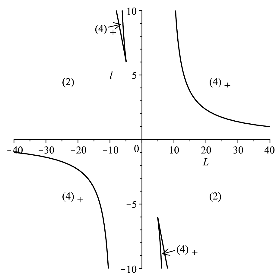
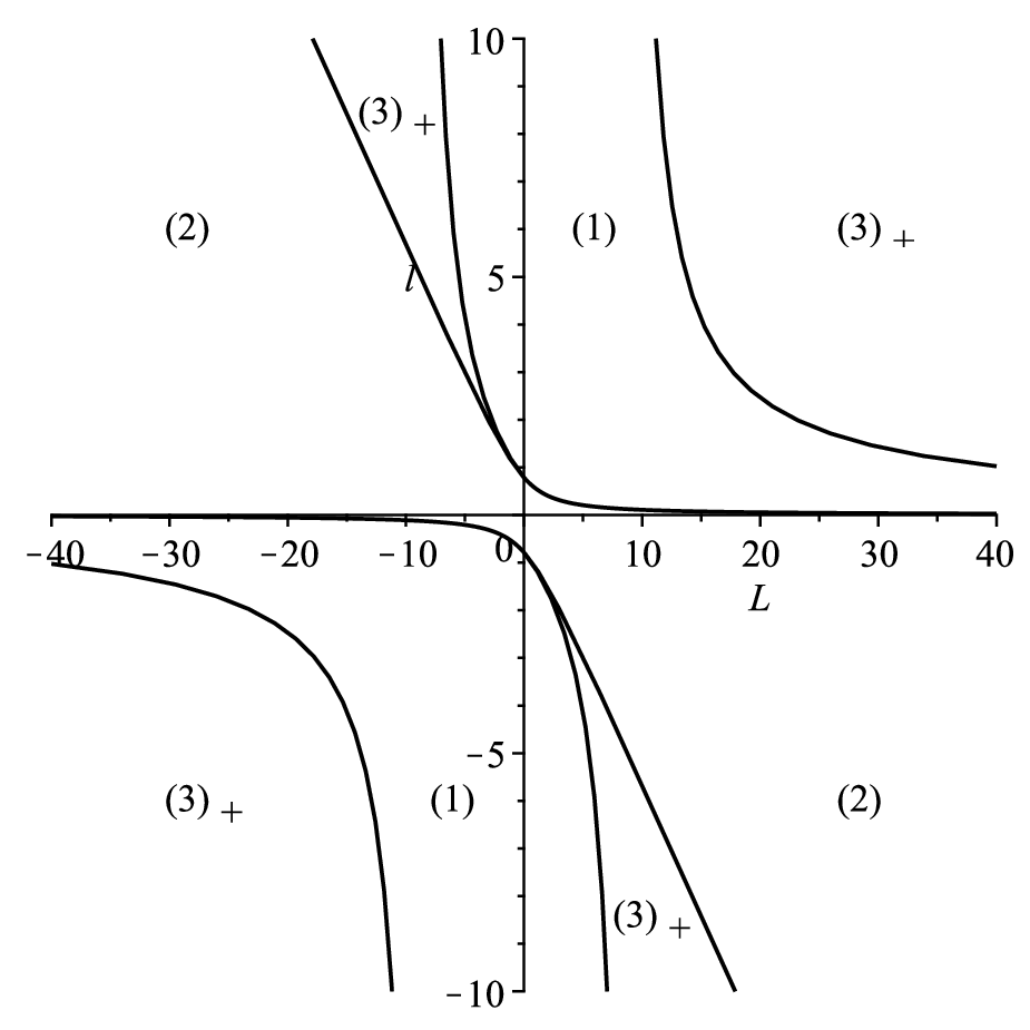
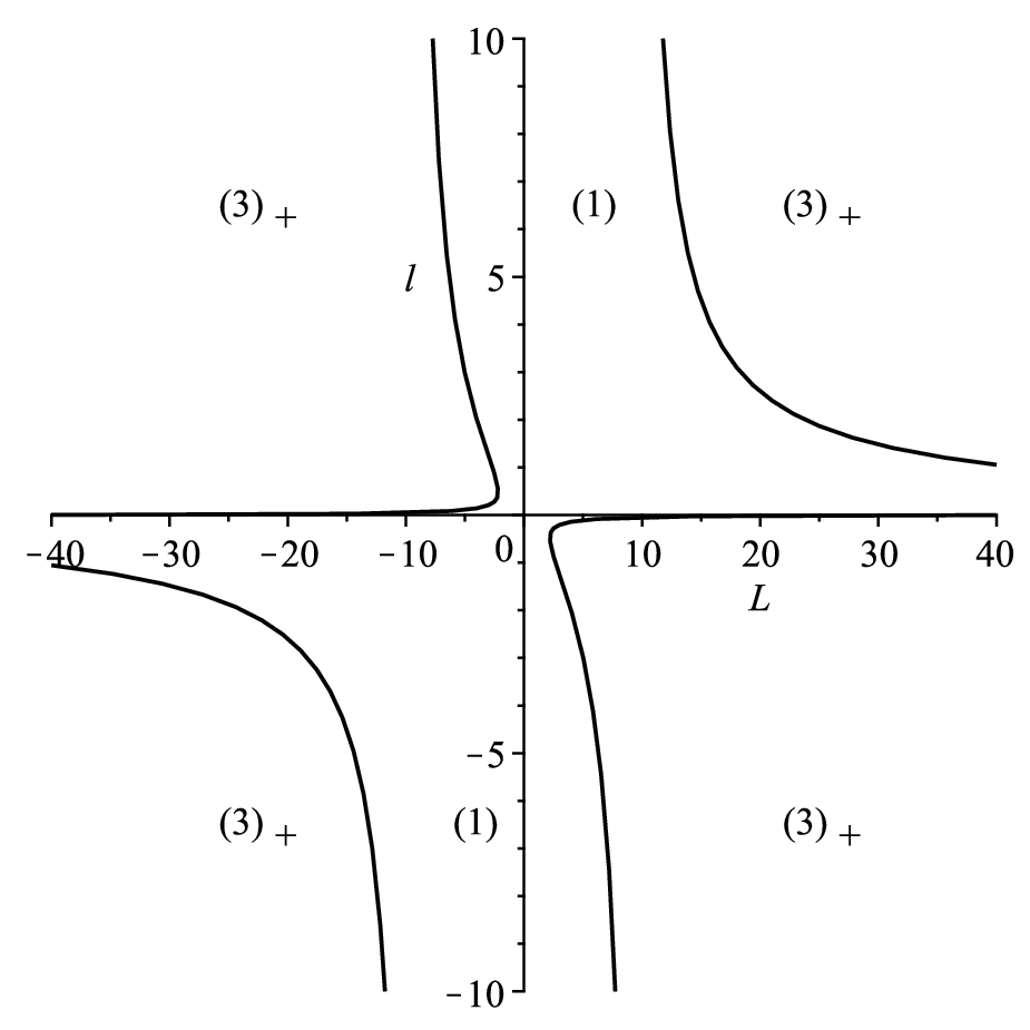
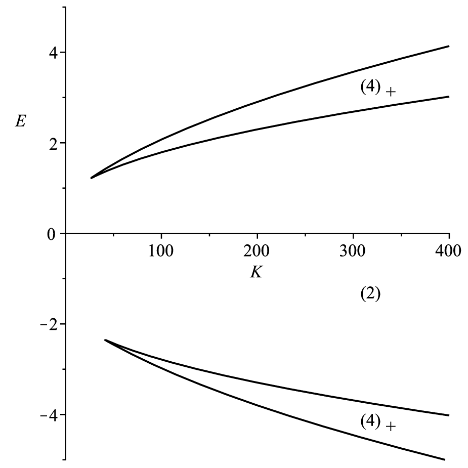
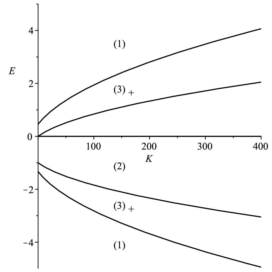
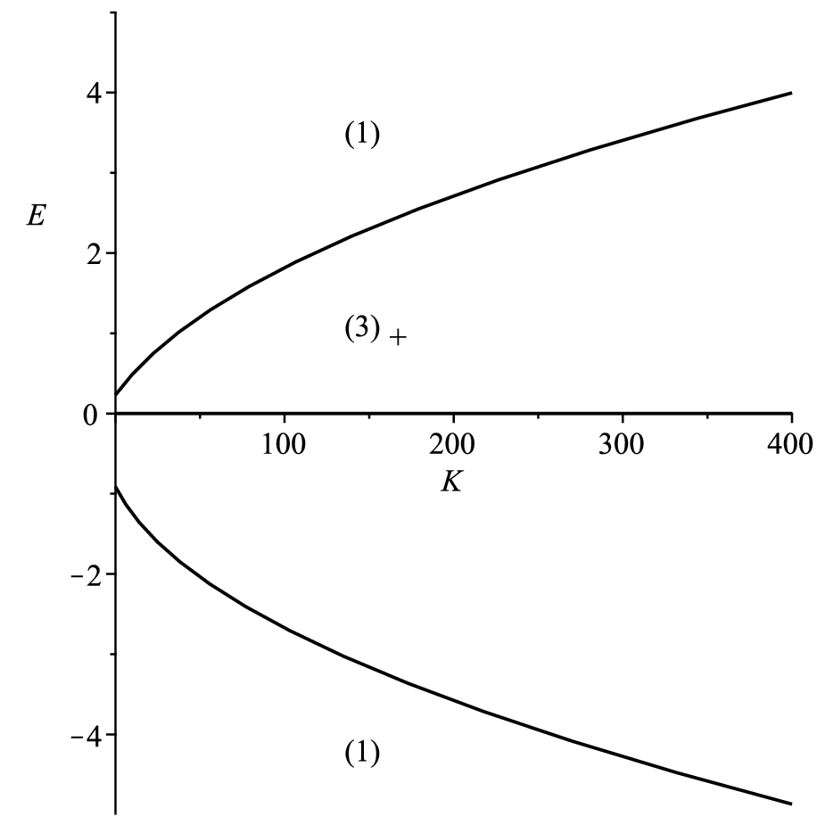
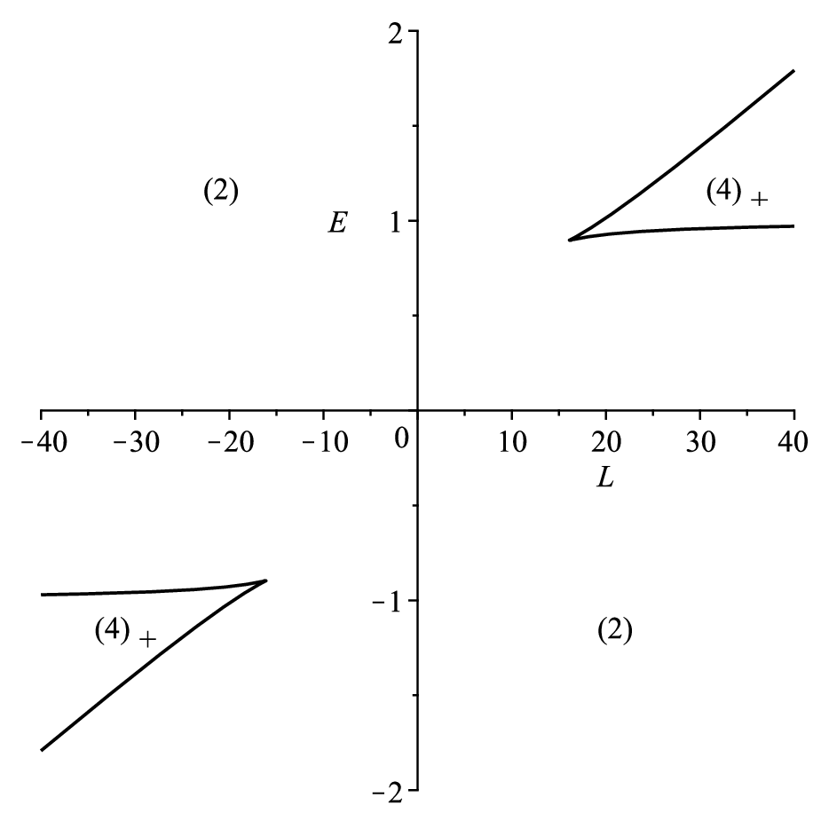
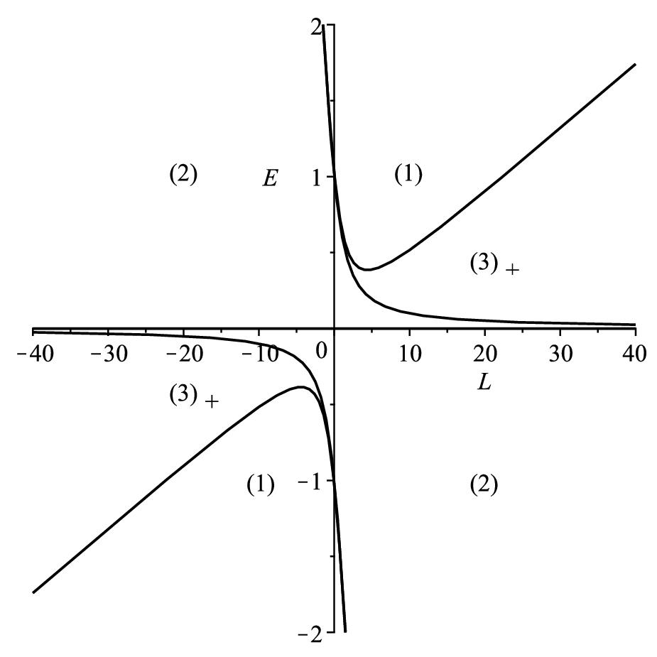
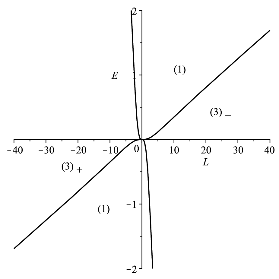
a variation of parameters is expected to change the number of positive zeros. By plotting the zeros of the resultant of the two expressions in Eq. (30), one obtains parameter plots showing the boundaries between regions of 1, 2, 3 or 4 zeros of P. This is shown for parametric -, -, and - diagrams in Fig. 2.
As P is a polynomial of second degree in , one can define the two-part effective potential as the values of energy that yield , i.e., P can be rearranged in the form
| (31) |
Some effective potentials are shown in Figs. 3–5. Since one can factor out in , and intersect on the horizon at , given that is real. Additionally, for the requirement that time should always run forward, i.e., , Eq. (24) is treated in a similar way as Eq. (20) for the effective potential and corresponding regions are shown as well.


Since for and for hold in the limit , orbits of particles of positive mass are always bounded, particles of imaginary mass can exist in unbound orbits for arbitrary energy. More precisely, one finds for particles of non zero mass, i.e., , in the limiting case from
| (32) |
Similarly, for massless particles, i.e., , it follows in the limit
| (33) |
Since here and hold (for ) and for in the limit , for every set of parameters a physically forbidden region in the vicinity of can be found. This behavior corresponds to the border of region (2) in Fig. 2(e) as varying the energy to region (3)+ allows for an additional unbound orbit.
In special cases, terminating orbits can be found. Due to the smoothness of the polynomial P, the condition has to be fulfilled, which implies real , since opens downward with respect to . It follows
| (34) |
giving and as first conditions. To allow for non trivial terminating orbits with non zero range, additionally has to hold on with . This implies that the lowest order non vanishing coefficient of P must be positive, which is a condition that is always met in case of but never possible in other cases. The influence of the choice of on the effective potential at the singularity around is shown in Fig. 4. Here parameters are chosen to allow for bound orbits behind the horizon for all particle masses . As regions with are shown as well, it can be seen that all depicted bound orbits cross regions where time is running backwards. For a particle of non zero mass this can be avoided by lowering its energy to the bottom of the potential well. A short-range terminating orbit can be found in Fig. 4(c) at . Additionally, the two possible types of terminating orbits can be seen in Figs. 5(a) and 5(b).
With the results of the parametric diagrams and the effective potentials we summarize all combinations of zeros of P and show their corresponding types of orbits in Table 1. Here the following connection of regions in the parametric diagrams and types of orbits was found:
- 1.
Region (1): P has one non negative zero , which corresponds to a TEO of type A. For particles of imaginary mass a TO of type is possible for an energy of [see, e.g., Fig. 5(a)].
- 2.
Region (2): P has two positive zeros , which corresponds to a MBO of type B.
- 3.
Region (3): P has three non negative zeros .
- (a)
Region : It holds , resulting in a MBO and an EO of type C.
- (b)
Region : For all zeros it holds , resulting in a BO and a TEO of type D. Again, for particles of imaginary mass a TO of type is possible for an energy of [see, e.g., Fig. 5(b)].
- (a)
- 4.
Region (4): P has four positive zeros .
- (a)
Region : It holds , resulting in a MBO and a BO of type E.
- (b)
Region : It holds , resulting in a BO and a MBO of type F.
- (a)
| Type | Region | Zeros | Range of | Orbit | |
|---|---|---|---|---|---|
| A | (1) | 1 | , 0 | TEO | |
| TO | |||||
| B | (2) | 2 | 0, 1 | MBO | |
| C | 3 | , 0 | MBO, EO | ||
| D | 3 | , 0 | BO, TEO | ||
| TO, TEO | |||||
| E | 4 | 1 | MBO, BO | ||
| F | 4 | 1 | BO, MBO |
Note that for every radially allowed orbit an angular momentum according to Section 3.1 can be chosen to allow for motion as well.
3.3 Static orbits
It has been shown in Collodel:2017end that some axisymmetric rotating spacetimes possess a ring in the equatorial plane, on which stationary particles remain stationary with respect to an asymptotic static observer. As this is possible in higher dimensions as well (see Collodel:2017end and references therein), we check whether this is the case for the spacetime at hand. Hence, parameters have to be chosen to allow for an extremum of at and a double zero in Eq. (29) at . Additionally, the right hand sides of Eqs. (22) and (23) have to vanish. We use from Eq. (29), under conditions discussed in Section 3.1, together with Eq. (23), from which the requirement and can be derived. With this, a turnaround energy can be defined by solving Eq. (22) for yielding
| (35) |
This is also shown in Figs. 4 and 5, since here holds. To obtain a stationary point, has to intersect in an extremum of . In this spacetime, we could not find such intersections. However, pointy petal BOs (in front of the horizon), semi BOs (behind the horizon) as well as MBOs, where the particle is periodically at rest, are found at arbitrary intersections of and for particles of positive mass. In case of a pointy petal BO, an effective potential and turnaround energy is shown in Fig. 5(c).
3.4 Spacelike geodesics and AdS/CFT
Spacelike geodesics are usually not considered in the analysis of geodesic motion, since they represent test particles with imaginary rest mass (). In the context of AdS/CFT, however, there are applications for spacelike geodesics. CFT correlators or Feynman propagators describe observables on the asymptotic boundary of an AdS spacetime. Correlation functions of fields in the bulk are related to correlation functions of CFT operators on the boundary. Using the Green function, the correlator of two operators can be written as
| (36) |
Here describes the proper length of the path between the boundary points and . In the case of spacelike trajectories is imaginary, so that the whole expression is real. is the mass of the bulk field, which is related to the conformal dimension of the Operator . For large masses, i.e., , the WKB approximation can be used to calulate the operator, which is then described by the sum over all spacelike geodesics between the boundary points
| (37) |
The real proper length of a geodesic diverges due to contributions near the AdS boundary and has to be renormalized by removing the divergent part in pure AdS. The sum is then dominated by the shortest spacelike geodesic between the boundary points (see, e.g., Balasubramanian:1999zv, Balasubramanian:2011ur, Louko:2000tp).
In this formalism we need geodesics that have endpoints on the boundary at . This is the case for escape orbits (EOs) and two-world escape orbits (TEOs) that have a single turning point and reach infinity. For EOs both endpoints of the geodesic are located on a single boundary, since the turning point is outside the horizons. The corresponding two-point correlators can be used to calculate for example the thermalization time Balasubramanian:2011ur or the entanglement entropy Hubeny:2007xt, AbajoArrastia:2010yt.
Particles on TEOs cross the horizon and therefore the endpoints are on two disconnected boundaries. TEOs can also be considered as propagators Balasubramanian:1999zv; Louko:2000tp. The boundary correlators can probe the physics behind the horizon. This could be used to study the formation of black holes Balasubramanian:1999zv, the black hole singularity Fidkowski:2003nf, or the information paradox Papadodimas:2012aq.
In the spacetime of a supersymmetric AdS5 black hole, geodesics relevant for AdS/CFT exist in the regions (1), (3)+ and (3)-, see Fig. 2 and Table 1. Depending on the parameters of the black hole, we find EOs or TEOs. In region (3)+ EOs exist that return to the same boundary where they started. In region (1) and (3)-, there are TEOs crossing the horizon with endpoints on two disconnected boundaries.
4 Solution of the geodesic equations
4.1 Solution of the equation
4.2 Solution of the equation
By substituting , with chosen to be a zero of P, one can simplify Eq. (20) to a differential equation of the type with a polynomial of third order on its right hand side (this step is not necessary for ). The following substitution transforms this to
| (39) |
with coefficients
| (40) |
This elliptic differential equation is solved by the Weierstrass function markushevich1967theory, which leads to
| (41) |
as a solution of Eq. (39). Here we set with and the initial value of . The solution of Eq. (20) is now obtained by
| (42) |
4.3 Solution of the equation
To integrate Eq. (22), we handle its two parts separately and set
| (43) |
Again, the substitution is used, this time upon . Together with Eq. (28), one gets for the part
| (44) |
Here the “” indicates the sign of . Upon the two fractions we apply partial fraction decompositions
| (45) |
The first part can be easily integrated with the substitution , the second part with . The third part is equal to , as can be seen from Eq. (28). This yields
| (46) | ||||
| (47) | ||||
where , with , , , and . Furthermore, was assumed.
Now we integrate the dependent part of Eq. (22). We use the two substitutions applied in Section 4.2 and recall Eq. (41) to identify . A partial fraction decomposition on is performed to get
| (48) |
where , and are constants of the partial fraction decomposition and and are poles of first order. According to Willenborg:2018zsv33 3 Here an incorrect index has been changed., the elliptic integrals of third kind can be solved in terms of the Weierstrass and functions by using addition theorems. One obtains with
| (49) |
Here is a Weierstrass transformed pole , which solves for in the fundamental parallelogram of .
4.4 Solution of the equation
4.5 Solution of the equation
The integral of the right hand side of Eq. (24) can be derived similarly to that of in Section 4.3. Here the partial fraction decomposition leads to
| (52) |
with , and given by the partial fraction decomposition and and are poles of first and second order, respectively, that are identical to those in Eq. (48). The integral of the first three terms yields an expression of the type obtained in Eq. (49). Again, according to Willenborg:2018zsv44 4 Here two incorrect signs have been changed., the elliptic integral of type can be solved in terms of the Weierstrass and functions. One obtains with and the initial value of
| (53) |
5 The orbits
To plot the spatial coordinates of the set of analytical solutions for the particle’s motion in a Cartesian coordinate system, a coordinate transformation has to be chosen. The angular line element for of the metric in Eq. (1) yields in case of
| (54) |
On the other hand, the angular line element of flatspace in biazimuthal coordinates is
| (55) |
A comparison of Eqs. (54) and (55) suggests the coordinate transformation
| (56) |
which, together with the biazimuthal coordinates and , transforms to by
| (57a) | ||||
| (57b) | ||||
| (57c) | ||||
| (57d) | ||||
Furthermore, we choose a projection in the 3-dimensional Cartesian subspace of the coordinates by setting . This preserves the notion of a horizon on the surface of a sphere with radius , but as a consequence we have to set , so only analytical solutions of and are used. Another consequence is that the motion on the interval is now mapped to the upper hemisphere only, thereby, as the horizon is shown in the following as a complete sphere of radius , the lower half sphere is of no physical relevance.
The figures below show the particle’s motion for various sets of parameters. The first orbit of a particle of positive mass is of type E and is shown in Fig. 6, its effective potential can be found in Fig. 3(d). For similar parameters ( was decreased) a lightlike orbit of type C is shown in Fig. 7. Both of those orbits pass the equatorial plane. An orbit that is confined to one hemisphere has to satisfy , as was discussed in Section 3.1. A lightlike orbit of this kind is shown in Fig. 8 for type C.
In case of and , one obtains an orbit confined to a cone of fixed opening angle . This is shown in Fig. 9 for type C. A two-world escape orbit of type A can be found in Fig. 10(a). This is obtained by increasing the energy slightly above the effective potential’s maximum while the other parameters are unchanged compared to Fig. 7. By the increase in energy, the many-world periodic bound orbit and the escape orbit merged into one two-world escape orbit.
Now we present orbits of particles with imaginary mass that reach the boundary at infinity and therefore are of relevance for AdS/CFT. A terminating orbit of type , with its effective potential depicted in Fig. 5(a), can be found in Fig. 10(c). In Fig. 11 we show a terminating orbit and a two-world escape orbit of type of a particle with imaginary mass in an effective potential very similar to the one shown in Fig. 5(b).
The pointy petal bound orbit of type E of a particle that is periodically at rest is depicted in Fig. 12, its effective potential in Fig. 5(c). Here parameters are chosen by determining the intersection of the effective potential and turnaround energy while is, for simplicity, chosen to be constant, as discussed in Section 3.3.
Finally, a bound orbit behind the horizon for a particle of positive mass (type F) is shown in Fig. 13. This requires small and large . Its effective potential is very similar to the one shown in Fig. 4(a) but its trajectory is not confined to a cone of fixed opening angle .


6 Conclusion
In this article the spacetime of a supersymmetric AdS5 black hole was studied by analyzing the geodesics (elliptic) equation of motion and deriving its analytical solutions in terms of the Weierstrass , , and functions. Effective potentials and parametric diagrams were used to classify possible types of orbits, which are characterized by the particle’s energy, angular momenta, Carter constant, and mass parameter as well as the metric’s AdS radius.
We showed that timelike orbits are always bounded and thus do not reach the AdS boundary. For lightlike and spacelike geodesics multiple types of orbits with a boundary at infinity and therefore with relevance for AdS/CFT were found. This, for spacelike geodesics and for a specific energy, includes the possibility of a terminating orbit. Bound orbits behind the horizon (for large angular momentum ) and many-world periodic bound orbits are possible independently of the particle’s mass. However, stable bound orbits outside of the horizon are only possible for particles of positive mass.
Future work might focus on extending the equations of motion to particles with electric and magnetic charge. Additionally, the orbits’ observables, e.g., in case of a bound orbit, its periastron shift or, in case of a lightlike escape orbit, its light deflection or the black hole’s shadow, might be calculated similarly as in Hackmann:2010zz by making use of the analytical solutions.
Acknowledgements.
We would like to thank Jutta Kunz and Lucas G. Collodel for fruitful discussions. We gratefully acknowledge support by the DFG (Deutsche Forschungsgemeinschaft/German Research Foundation) within the Research Training Group 1620 “Models of Gravity”.References
- (1) J.M. Maldacena, Int. J. Theor. Phys. 38, 1113 (1999). DOI 10.1023/A:1026654312961,10.4310/ATMP.1998.v2.n2.a1. [Adv. Theor. Math. Phys.2,231(1998)]
- (2) R.P. Kerr, Phys. Rev. Lett. 11, 237 (1963). DOI 10.1103/PhysRevLett.11.237
- (3) B. Carter, Commun. Math. Phys. 10(4), 280 (1968). DOI 10.1007/BF03399503
- (4) S.W. Hawking, C.J. Hunter, M. Taylor, Phys. Rev. D59, 064005 (1999). DOI 10.1103/PhysRevD.59.064005
- (5) J.B. Gutowski, H.S. Reall, JHEP 02, 006 (2004). DOI 10.1088/1126-6708/2004/02/006
- (6) J.P. Gauntlett, J.B. Gutowski, S. Pakis, JHEP 12, 049 (2003). DOI 10.1088/1126-6708/2003/12/049
- (7) M. Cvetic, G.W. Gibbons, H. Lu, C.N. Pope, (2005)
- (8) V. Balasubramanian, S.F. Ross, Phys. Rev. D61, 044007 (2000). DOI 10.1103/PhysRevD.61.044007
- (9) G.V. Kraniotis, Class. Quant. Grav. 22, 4391 (2005). DOI 10.1088/0264-9381/22/21/001
- (10) G.V. Kraniotis, Class. Quant. Grav. 24, 1775 (2007). DOI 10.1088/0264-9381/24/7/007
- (11) R. Fujita, W. Hikida, Class. Quant. Grav. 26, 135002 (2009). DOI 10.1088/0264-9381/26/13/135002
- (12) E. Hackmann, V. Kagramanova, J. Kunz, C. Lammerzahl, EPL 88(3), 30008 (2009). DOI 10.1209/0295-5075/88/30008
- (13) E. Hackmann, C. Lammerzahl, V. Kagramanova, J. Kunz, Phys. Rev. D81, 044020 (2010). DOI 10.1103/PhysRevD.81.044020
- (14) S. Grunau, H. Neumann, S. Reimers, Phys. Rev. D97(4), 044011 (2018). DOI 10.1103/PhysRevD.97.044011
- (15) G.W. Gibbons, C.A.R. Herdeiro, Class. Quant. Grav. 16, 3619 (1999). DOI 10.1088/0264-9381/16/11/311
- (16) V. Diemer, J. Kunz, Phys. Rev. D89(8), 084001 (2014). DOI 10.1103/PhysRevD.89.084001
- (17) J.C. Breckenridge, R.C. Myers, A.W. Peet, C. Vafa, Phys. Lett. B391, 93 (1997). DOI 10.1016/S0370-2693(96)01460-8
- (18) A. Ashtekar, S. Das, Class. Quant. Grav. 17, L17 (2000). DOI 10.1088/0264-9381/17/2/101
- (19) I. Papadimitriou, K. Skenderis, JHEP 08, 004 (2005). DOI 10.1088/1126-6708/2005/08/004
- (20) B. Carter, Phys. Rev. 174, 1559 (1968). DOI 10.1103/PhysRev.174.1559
- (21) Y. Mino, Phys. Rev. D67, 084027 (2003). DOI 10.1103/PhysRevD.67.084027
- (22) S. Grunau, V. Kagramanova, Phys. Rev. D83, 044009 (2011). DOI 10.1103/PhysRevD.83.044009
- (23) L.G. Collodel, B. Kleihaus, J. Kunz, Phys. Rev. Lett. 120(20), 201103 (2018). DOI 10.1103/PhysRevLett.120.201103
- (24) V. Balasubramanian, A. Bernamonti, J. de Boer, N. Copland, B. Craps, E. Keski-Vakkuri, B. Muller, A. Schafer, M. Shigemori, W. Staessens, Phys. Rev. D 84, 026010 (2011). DOI 10.1103/PhysRevD.84.026010
- (25) J. Louko, D. Marolf, S.F. Ross, Phys. Rev. D 62, 044041 (2000). DOI 10.1103/PhysRevD.62.044041
- (26) V.E. Hubeny, M. Rangamani, T. Takayanagi, JHEP 07, 062 (2007). DOI 10.1088/1126-6708/2007/07/062
- (27) J. Abajo-Arrastia, J. Aparicio, E. Lopez, JHEP 11, 149 (2010). DOI 10.1007/JHEP11(2010)149
- (28) L. Fidkowski, V. Hubeny, M. Kleban, S. Shenker, JHEP 02, 014 (2004). DOI 10.1088/1126-6708/2004/02/014
- (29) K. Papadodimas, S. Raju, JHEP 10, 212 (2013). DOI 10.1007/JHEP10(2013)212
- (30) A. Markushevich, R. Silverman, Theory of functions of a complex variable. No. Bd. 3 in Selected Russian publications in the mathematical sciences
- (31) F. Willenborg, S. Grunau, B. Kleihaus, J. Kunz, Phys. Rev. D97(12), 124002 (2018). DOI 10.1103/PhysRevD.97.124002