Geometric partition categories:
On short Brauer algebras and their blob subalgebras

Z. KÁDÁR P. P. MARTIN Affiliation: School of Mathematics, University of Leeds

Abstract: The main result here gives an algebra(/linear category) isomorphism between a geometrically defined subcategory ${\mathcal{J}}^{1}_{0}$ of a short Brauer category ${\mathcal{J}}_{0}$ and a certain one-parameter specialisation of the blob category ${\mathfrak{b}}$ . That is, we prove the Conjecture in Remark 6.7 of [14]. We also define a sequence of generalisations ${\mathcal{J}}^{i}_{i-1}$ of the category ${\mathcal{J}}^{1}_{0}$ . The connection of ${\mathcal{J}}_{0}$ with the blob category inspires a search for connections also with its beautiful representation theory. Here we obtain formulae determining the non-semisimplicity condition (generalising the classical ‘root-of-unity’ condition).

Keywords: diagram algebra, topological spin chain.

1 Introduction

A motivating aim here is to study the structure of the $k$ -linear categories ${\mathcal{J}}_{l}$ from [14], and in particular the representation theory of the corresponding $k$ -algebras (with $k$ a field) ${\mathcal{J}}_{l,n}$ in the non-semisimple cases. These structures are of intrinsic interest (cf. [11, 12, 21, 8]); and see also [14] for a discussion of some of the extrinsic motivations for this study — in short one seeks generalisations of the intriguing examples of Kazhdan–Lusztig theory [15, 29, 2] observed [21] in the representation theory of the Brauer category ${\mathcal{B}}={\mathcal{J}}_{\infty}$ [6]. Another motivating aim is to study module categories over monoidal categories (see e.g. [26] for a review) beyond the usual ‘semisimple’ setting.

The study strategy in Part 1 (§2-4) can be seen as trying to relate the problem to the representation theory of the blob category ${\mathfrak{b}}$ and the blob algebra ${\mathfrak{b}}_{n}$ [22], which is contrastingly very well understood (see e.g. [9]), itself with deep and tantalising connections to Kazhdan–Lusztig theory [23]. (More recently see e.g. [5].) This also allows us to make contact with the original physical motivations for these algebras, as the algebras of physical systems with boundaries and interfaces [22]. Indeed the blob algebras have been of renewed interest recently in several areas, not only of physics but also for example the study of KLR algebras [16, 28], Soergel bimodules [30] and monoidal categories [13].

As we shall see, in the simplest non-trivial case the algebras are (at least) related by inclusions of the form ${\mathfrak{b}}_{m}\hookrightarrow{\mathcal{J}}_{0,n}$ . Inclusion is not in general a directly helpful relationship in representation theory. (For example the Temperley–Lieb algebra $T_{n}$ [31] is a subalgebra of ${\mathfrak{b}}_{n}$ , but the representation theories of these algebras are radically different: cf. [19] and [9].) However the inclusion here is of ‘high index’, so there is hope that it will indeed shed light on the open problem.

In Part 2 (§5) we include some indicative results on ${\mathcal{J}}_{0,n}$ representation theory. These are obtained by working directly with ${\mathcal{J}}_{0,n}$ , but serve as a first step in this direction (full analysis of these results is demoted to a separate paper).

In Section 2 we introduce concepts and notations. In §3 we define for each category ${\mathcal{J}}_{l}$ a new subcategory. In §4 we examine the relationship to the blob category. In particular in Section 4 we state and prove the main theorem. In section 5 we consider consequences for the algebras ${\mathcal{B}}^{l}_{n}={\mathcal{J}}_{l,n}$ themselves. In Section 6 we discuss related open problems.

2 Preliminary definitions

Define $\underline{n}=\{1,2,...,n\}$ , $\underline{n}^{\prime}=\{1^{\prime},2^{\prime},...,n^{\prime}\}$ and so on. Define $V^{n}_{m}=\underline{n}\cup\underline{m}^{\prime}$ . Write $J(n,m)$ for the set of set partitions of $\underline{n}\cup\underline{m}^{\prime}$ into subsets of order 2. Fix a commutative ring $k$ and $\delta\in k$ . In §2.1-2.2 we recall the Brauer partition category

{{\mathcal{B}}}=({\mathbb{N}}_{0},kJ(n,m),*)

with loop-parameter $\delta$ . The category ${\mathcal{B}}$ has an infinite family of subcategories ${\mathcal{J}}_{l}$ introduced in [14]. The key ingredient in [14] is the definition of the left-height of a partition. We recall it here in §2.3. In §2.4, we recall the blob category [22].

2.1 Brauer picture calculus

Refer to caption — Figure 1: A regular intersection between lines (circled).

We recall the definition of multiplication $*$ in ${{\mathcal{B}}}$ and relate to ‘pictures’ of partitions.

(2.1) Fix a dimension $d>0$ . Given an ordered list $r=(r^{1},r^{2},...,r^{l})$ of points in ${\mathbb{R}}^{d}$ , let

(r)=\bigcup_{i=1}^{l-1}[r^{i},r^{i+1}]

where $[r^{i},r^{i+1}]\subset{\mathbb{R}}^{d}$ is the straight line between these points.

A line or polygonal path in the plane ${\mathbb{R}}^{2}$ is a subset of form $(r)$ such that each point $r^{i}$ lies in at most two of the straight lines.

(2.2) Let $R\subset{\mathbb{R}}^{2}$ be a rectangle, with frame $\partial R$ and interior $(R)=R\setminus\partial R$ . A set of lines is regular in $R$ if:
(R1) each line $(r)\subset R$ touches $\partial R$ only if $r^{1}\neq r^{l}$ and then only at its end-points $r^{1},r^{l}$ ;
(R2) the point-list $r^{1},r^{2},...,r^{l}$ of each line has no intersection with any other line. See Fig. 1.

(2.3) Remark. Given a regular set of lines $D$ , consider the subset $p(D)$ of $R$ defined by $D$ . Note that we can recover the points of $D$ from $d=p(D)$ except for those points $r^{i}$ that are colinear with their neighbours $r^{i-1},r^{i+1}$ . Note that colinearity is not a generic condition. The fibre $p^{-1}(d)$ of regular sets of lines over $d$ includes a representative $D^{\prime}$ in which no line has an $i$ with $r^{i-1},r^{i},r^{i+1}$ colinear. The fibre consists of sets obtained by inserting such colinear points in lines.

Note that $d$ completely determines $D$ up to such inserted colinear points.

(2.4) A Brauer picture $d$ of a partition $p$ in $J(n,m)$ is a rectangle $R\subset{\mathbb{R}}^{2}$ with $n$ points (called ‘vertices’) labeled $1,2,...,n$ on the northern edge, and $m$ on the southern edge (as in Figure 2); and a subset of $R$ consisting of a regular set of lines $(r)$ in $R$ as follows. Each line is either a loop ( $r^{1}=r^{l}$ ) or else connects vertices pairwise in accordance with the pairs in $p$ .

See Fig.2 and Fig.3 for examples. Remark: As far as physically drawn figures are concerned, piecewise linear and piecewise smooth lines are effectively indistinguishable, by [24, §6] for example.

(2.5) Note that the construction ensures a well-defined map $\pi$ from pictures to partitions: for each $i\in V^{n}_{m}$ the line from $i$ in $d$ may be followed unambiguously to the other end; and one takes a line with end-points $i,j$ to $\{i,j\}$ .

(2.6) For $p\in J(n,m)$ write $[p]$ for the set of pictures $d$ such that $\pi(d)=p$ . Note that every $[p]$ is non-empty. Write $\#(d)$ for the number of loops in picture $d$ .

(2.7) Recall $\delta\in k$ . We extend the $\pi$ -map to $\Pi(d)=\delta^{\#(d)}\pi({d})\in kJ(m,n)$ .

For $d$ a picture let $\hat{d}$ denote $d$ with all loops removed. Thus $\Pi(d)=\delta^{\#(d)}\Pi(\hat{d})$ .

(2.8) Consider pictures $d_{1}$ for $p_{1}\in J(m,n)$ and $d_{2}$ for $p_{2}\in J(n,q)$ .

We have not specified exactly where the $n$ vertices lie on the southern frame of $R$ in $d_{1}$ (or indeed where the southern frame lies in ${\mathbb{R}}^{2}$ ), but it will be clear that there are representative pictures of $p_{1},p_{2}$ for which the $n$ vertices from $d_{1}$ match up with the $n$ from $d_{2}$ . These pictures can then be stacked (with $d_{1}$ over $d_{2}$ ) so that the $n$ vertex sets in each ‘factor’ coincide. Note that the concatenation is again a Brauer picture. It is denoted by $d_{1}\,|\,d_{2}$ .

Note then (1) that $d_{1}|d_{2}$ can be seen as a picture of an element of $kJ(m,q)$ ;
(2) that if $d_{2}$ and $d_{3}$ also stack then

(d_{1}|d_{2})|d_{3}=d_{1}|(d_{2}|d_{3})

(1)

2.2 The Brauer partition category ${\mathcal{B}}$

Given a set $p$ of symbols, let $p^{\prime}$ be the set obtained by adding primes to symbols in $p$ (note that this can work recursively). For example $\{\{1,2\},\{3,2^{\prime}\},\{1^{\prime},3^{\prime}\}\}^{\prime}=\{\{1^{\prime},2^{\prime}\},\{3^{\prime},2^{\prime\prime}\},\{1^{\prime\prime},3^{\prime\prime}\}\}$ .

(2.9) Let $p_{1}\in J(m,n)$ and $p_{2}\in J(n,q)$ . Now form $p_{1}\cup p_{2}^{\prime}$ . Note that $p_{1}$ and $p_{2}^{\prime}$ may not be quite disjoint in general. When a primed pair in $p_{1}$ meets the corresponding unprimed pair from $p_{2}$ the union ‘flattens’ this to a single pair. Note each single-primed element appears twice (or once if flattened) and others once. Consider a maximal chain $\{a_{0},a_{1}\},\{a_{1},a_{2}\},...,\{a_{k-1},a_{k}\}$ in $p_{1}\cup p_{2}^{\prime}$ . The chain is either all primed, and $a_{0}=a_{k}$ or $k=1$ ; or else $\{a_{0},a_{k}\}$ lies in $\underline{m}\cup\underline{q}^{\prime\prime}$ (to which we may apply $i^{\prime\prime}\leadsto i^{\prime}$ to obtain an element of $\underline{m}\cup\underline{q}^{\prime}$ ). In this way $p_{1}\cup p_{2}^{\prime}$ determines an element $p_{1}.p_{2}$ of $J(m,q)$ ; and also a number $\#$ of all-primed ‘closed’ chains. Define

p_{1}*p_{2}=\;\delta^{\#}p_{1}.p_{2}\;\in kJ(m,q).

Note that if $d_{i}\in[p_{i}]$ and $d_{1}|d_{2}$ then
(I) each maximal chain above corresponds to vertices in a line component of $d_{1}|d_{2}$ .
(II) the pair $\{a_{0},a_{k}\}$ corresponds to the vertices at the ends of the line component of $d_{1}|d_{2}$ . Thus the image in $\pi(d_{1}|d_{2})$ if $a_{0}\neq a_{k}$ is $\{a_{0},a_{k}\}$ (more precisely $\{a_{0},a_{k}\}$ with any $i^{\prime\prime}\leadsto i^{\prime}$ ).

(2.10) From the notes (I,II) in (2.2) we have, independently of the choice of pictures,

p_{1}*p_{2}=\Pi(d_{1}\,|\,d_{2}).

For example, from Figure 4 (ignoring the red line for now)

\{\{4^{\prime},2\},\{3,5^{\prime}\},\{1,3^{\prime}\},\{1^{\prime},2^{\prime}\}\}*\{\{2,1\},\{4,5\},\{1^{\prime},3\}\}\;=\;\delta\{\{3,2\},\{1,1^{\prime}\}\}\;\in kJ(3,1)\ .

Note we use the convention that a picture $d_{1}$ for $p_{1}\in J(m,n)$ has $m$ (resp. $n$ ) points on its northern (southern) edge. Thus $d_{1}\,|\,d_{2}$ is the concatenation of $d_{1}$ on top of $d_{2}$ .

(2.11) Theorem.

[14] Composition $*$ is associative. This defines the category ${\mathcal{B}}$ .

Proof.

By the points (I,II) in (2.2) above we may obtain $p_{1}*p_{2}$ from $d_{1}|d_{2}$ (independently of the choices of these pictures). Existence of constructs of form $d_{1}|(d_{2}|d_{3})$ will be evident. Associativity follows since $(d_{1}|d_{2})|d_{3}=d_{1}|(d_{2}|d_{3})$ . (Alternatively we may stay with the initial machinery of (2.2) and simply introduce more primes. The pictures can be seen as bookkeeping the primes.) ∎

(2.12) Define $\otimes:J(n,m)\times J(n^{\prime},m^{\prime})\rightarrow J(n+n^{\prime},m+m^{\prime})$ as the composition corresponding to side-by-side concatenation of pictures. Note the following.

(2.13) Lemma.

(I) The composition $\otimes$ makes ${\mathcal{B}}$ into a monoidal category.
(II) Let $w\in J(n,m)$ for some $n,m$ , with $J(n,m)\hookrightarrow kJ(n,m)$ in the natural way. Then $p\otimes w=q\otimes w$ implies $p=q$ . ∎

2.3 The subcategory ${\mathcal{J}}_{l}$ of category ${\mathcal{B}}$

The regularity property (R2) of a picture $d$ means that the number, and position, of crossings of lines in $d$ is well-defined. A path through a picture $d$ is a further line in $R$ that satisfies (R2).

Fix a picture $d$ , let $x$ be a point in $d$ , and consider all paths from $x$ to the left edge. Then ‘left-height’ $h_{d}(x)$ is the minimum number of crossings with lines of the picture among such paths.

The left-height $h(d)$ of a picture $d$ is the maximum $h_{d}(x)$ of all crossing points $x$ of lines in $d$ ; or, if there are no crossings, then $h(d)=-1$ .

For $p\in J(n,m)$ let $h(p)$ denote the minimum $h(d)$ among pictures in $[p]=\{d:\pi(d)=p\}$ . Define

J_{\leq l}(n,m)=\{p\in J(n,m)\;|\;h(p)\leq l\}

Define $[p]^{\prime}$ as the subset of $[p]$ of pictures of $p$ of the minimum height. That is,

[p]^{\prime}=\{d\in[p]\;|\;h(d)=h(p)\}.

See Fig.3 for examples of minimum height pictures.

As shown in [14], $h(p_{1}*p_{2})\leq\max(h(p_{1}),(h(p_{2}))$ . A consequence is the following.

(2.14) Theorem.

[14] Category ${{\mathcal{B}}}$ has a subcategory ${\mathcal{J}}_{l}=({\mathbb{N}}_{0},kJ_{\leq l}(n,m),*)$ . ∎

(2.15) Given a subset $S$ of a rectangle $R$ , an alcove of $S$ is a connected component of $R\setminus S$ .

(2.16) Remark. Let $d\in[p]$ . Note that alcoves of $d$ have well-defined left-height. Note that the left-heights of the intervals of the frame of $R$ are determined by $p$ , and are otherwise independent of $d$ .

Proof: Note that there exist paths $w$ from the left edge of $R$ to points on $\partial R$ such that $w$ lies in a neighbourhood of $\partial R$ . Note (e.g. from the Jordan Curve Theorem) that there are such paths that have the lowest number of crossings. By construction two pictures $d,d^{\prime}\in[p]$ are close to identical in a neighbourhood of $\partial R$ . In particular there are paths to points on $\partial R$ that lie in such a neighbourhood; have the lowest number of crossings; and that have the same number of crossings in $d$ and $d^{\prime}$ . ∎

2.4 The blob category ${\mathfrak{b}}$

Now we recall the blob category [22]. Note that for $p\in J_{-1}(m,n)$ a pictures $d$ in $[p]^{\prime}$ has no crossings. Thus for each pair $v$ in $p$ the corresponding line $l_{v}$ in $d\in[p]^{\prime}$ has the property that every point $x$ on $l_{v}$ has the same value of $h_{d}(x)$ . Furthermore this $h_{d}(l_{v})=h_{d}(x)$ depends only on $v$ in $p$ and not on $d$ . Thus $v$ has a well-defined $h(v)=h_{d}(l_{v})$ . A left-exposed pair in $p\in J_{-1}(m,n)$ is a pair $v$ with $h(v)=0$ . (That is, there exists a path from the left edge of $R$ to $l_{v}$ , which path does not intersect any line of $d$ , for $d\in[p]^{\prime}$ . The line $l_{v}$ is literally left-exposed.)

(2.17) Lemma.

Let $p_{1}\in J_{-1}(m,n)$ and $p_{2}\in J_{-1}(n,q)$ . Let $d_{i}\in[p_{i}]^{\prime}$ . Let $v$ be a left-exposed pair in $p_{1}$ or $p_{2}$ and let $l_{v}$ be the corresponding line in $d_{i}$ . Then the line $l$ in $d_{1}\,|\,d_{2}$ containing $l_{v}$ has $h_{d}(l)=0$ .

Proof.

A path connecting the line $l_{v}$ to the left edge without intersection in $d_{1}$ or $d_{2}$ also connects the line in $d_{1}|d_{2}$ which contains $l_{v}$ to the left edge without intersection (cf. Fig.4). ∎

(2.18) For $p\in J_{-1}(m,n)$ let $S^{L}_{p}$ denote the subset of left-exposed pairs. Define

{{\mathsf{J}}^{\bullet}}(m,n)\;=\;\{(p,s)\,|\,p\in J_{-1}(m,n),\;s\subset S^{L}_{p}\}

(2)

(2.19) Let $(p_{1},s_{1})\in{{\mathsf{J}}^{\bullet}}(m,n)$ and $(p_{2},s_{2})\in{{\mathsf{J}}^{\bullet}}(n,q)$ . Recall $p_{1}.p_{2}$ and $p_{1}*p_{2}$ from (2.2). Define $\overline{s_{1}s_{2}}$ to be the set of those pairs $\{a_{0},a_{k}\}$ in $p_{1}.p_{2}$ , from chains $\{a_{0},a_{1}\},\{a_{1},a_{2}\},\dots,\{a_{k-1},a_{k}\}$ where at least one pair comes (in the obvious sense) from $s_{1}$ or $s_{2}$ . Define $\#$ as the number of closed chains with no pair from $s_{1},s_{2}$ , and $\#^{\prime}$ as the number of remaining closed chains.

We fix $\delta,\delta^{\prime}\in k$ and define the composition $\circ:{{\mathsf{J}}^{\bullet}}(m,n)\times{{\mathsf{J}}^{\bullet}}(n,q)\to k{{\mathsf{J}}^{\bullet}}(m,q)$ by

(p_{1},s_{1})\circ(p_{2},s_{2})=\;\delta^{\#}\delta^{\prime\#^{\prime}}(p_{1}.p_{2},\overline{s_{1}s_{2}}).

(2.20) Theorem.

Fix a commutative ring $k$ and $\delta,\delta^{\prime}\in k$ . Then ${\mathfrak{b}}=(\mathbb{N}_{0},k{{\mathsf{J}}^{\bullet}}(n,m),\circ)$ is a category.

Proof.

We require to prove associativity of the product, and this follows analogously to (2.2) and (2.11). Again the bookkeeping of extra primes may be seen from suitable pictures.

(2.21) A picture with blobs is a pair $(d,b)$ where $d$ is a picture in the sense of (2.1); and $b$ is a set of points (called blobs) in the interiors of lines of $d$ . We require that each blob lies in exactly one line (if $d\in[p]^{\prime}$ with $p\in J_{-1}$ then lines here are non-crossing and this is automatic).

(2.22) Given a picture with blobs $(d,b)$ such that $h_{d}(x\in b)=0$ we define

\pi^{\prime}:(d,b)\mapsto(\pi(d),s(b))\;\in{{\mathsf{J}}^{\bullet}}(m,n)

where $\pi$ is as in (2.1) and $s(b)$ is the set of pairs associated to the lines decorated by $b$ .

(2.23) An element $(p,s)\in{{\mathsf{J}}^{\bullet}}(m,n)$ can be represented by a pair $(d,b)$ , where $d$ is a no-loop picture of $p$ ; and $b$ consists of at least one point in the interior of each line of $d$ corresponding to a pair in $s$ . See Fig.5.

For an example note that Figure 5 is a picture $(d,\{P_{1},P_{2},P_{3}\})$ for an element

(p,s)=(\{\{2^{\prime},1^{\prime}\},\{9,10\},\{3,4\},\{7^{\prime},5\},\{1,2\},\{8,8^{\prime}\},\{3^{\prime},6^{\prime}\},\{5^{\prime},4^{\prime}\},\{6,7\}\},\;\{\{5,7^{\prime}\},\{1,2\},\{6^{\prime},3^{\prime}\}\})

$\in{{\mathsf{J}}^{\bullet}}(10,8)$ . The blobs $P_{i},i=1,2,3$ are mapped to the pairs $\{2,1\}$ , $\{5,7^{\prime}\}$ , $\{6^{\prime},3^{\prime}\}$ respectively.

(2.24) Define

\Pi(d,b)\;\;:=\;\;\delta^{\#(d,b)}\delta^{\prime\#^{\prime}(d,b)}\;\pi^{\prime}({d},{b})\;\;\in k{{\mathsf{J}}^{\bullet}}(m,n),

where $\#(d,b)$ (respectively $\#^{\prime}(d,b)$ ) is the number of loops without (respectively with) blobs.

Let $d_{i}\in[p_{i}]^{\prime}$ and $(d_{i},b_{i})$ be no-loop pictures with appropriate blobs (hereafter we just write $d_{i}$ , including blobs). By Lem.2.17 the concatenated picture $d_{1}\,|\,d_{2}$ is a picture of some $p\in J(m,q)$ plus possible loops and blobs. By an argument similar to (2.2) we have, independently of choices,

(p_{1},s_{1})\circ(p_{2},s_{2})=\;\Pi(d_{1}|d_{2}).

Existence of constructs of form $d_{1}|(d_{2}|d_{3})$ will again be evident. Since again $d_{1}|(d_{2}|d_{3})=(d_{1}|d_{2})|d_{3}$ we are done. ∎

(2.24.1) Corollary.

The End sets $k{{\mathsf{J}}^{\bullet}}(m,m)$ have the structure of an associative algebra.

We may denote these algebras by $J^{\bullet\,\delta,\delta^{\prime}}_{m}$ , or simply ${\mathfrak{b}}_{m}$ , indicating the fixed parameters from $k$ in the definition of the multiplication only when needed for clarity.

(2.25) Examples. Consider Fig.6(a,b). Applying the rules of multiplication we have e.g., $1e=e1=ee=e$ , $\;f_{1}^{2}=\delta f_{1}$ , $f_{2}^{2}=\delta^{\prime}f_{2}$ , $f_{2}f_{1}=f_{2}f_{3}=\delta^{\prime}f_{1}$ , $f_{6}f_{1}=f_{6}f_{3}=f_{3}$ and so on.

2.5 Generators and relations

(2.26) Theorem.

[22, 20] Consider the algebra defined by generators $U^{e}=\{e,U_{1},U_{2},...,U_{n-1}\}$ and relations
$\tau^{\prime}=\{\mbox{ $U_{i}^{2}=\delta U_{i}$, $U_{i}U_{i\pm 1}U_{i}=U_{i}$, $U_{i}U_{j}=U_{j}U_{i}$, $j\neq i\pm 1$, $ee=e$, $U_{1}eU_{1}=\delta^{\prime}U_{1}$, $U_{i}e=eU_{i}$, $i>1$ }\}$ . (I) The map

U_{i}\mapsto\{\underbrace{\{\{1,1^{\prime}\}\{2,2^{\prime}\},...,\{i,i+1\},\{i^{\prime},i+1^{\prime}\},...,\{n,n^{\prime}\}\}}_{p},\underbrace{\emptyset}_{s}\}

e\mapsto\{\underbrace{\{\{1,1^{\prime}\},\{2,2^{\prime}\},...,\{n,n^{\prime}\}\}}_{p},\underbrace{\{\{1,1^{\prime}\}\}}_{s}\}\hskip 72.26999pt

extends to an algeba isomorphism $k\langle U^{e}\rangle/\tau^{\prime}\cong{\mathfrak{b}}_{n}$ .
(II) Every element of the partition basis ${{\mathsf{J}}^{\bullet}}(n,n)$ can be expressed as a word in these generators. In particular $(p,s)\in{{\mathsf{J}}^{\bullet}}(n,n)$ can be expressed as a word in which $e$ appears as a factor $|s|$ times. ∎

2.6 Generator algebras $B_{l,m,n}$ and spin chain Physics

The original motivation for the blob algebra [22] was to study XXZ spin chains (and other related spin chains [1, 18]) with various boundary conditions via representation theory. In the simplest formulation (see [27, 17, 22] for details) one notes that there are boundary conditions for which the $n$ -site XXZ chain Hamiltonian may be expressed in the form

H=\sum_{i=1}^{n-1}U_{i}

where $U_{i}$ acts on $(\mathbb{C}^{2})^{n}$ by

U_{i}=1_{2}\otimes 1_{2}\otimes...\otimes\left(\begin{array}[]{cccc}0\\ &q&1\\ &1&q^{-1}\\ &&&0\end{array}\right)\otimes 1_{2}\otimes...\otimes 1_{2}

It is known that these matrices give a faithful representation of the Temperley–Lieb algebra. In this sense the algebra controls the spectrum of $H$ . A centraliser algebra is $U_{q}sl_{2}$ , and so this can equivalently be seen as controlling the spectrum.

There are several reasons for wanting to generalise away from this particular choice of boundary conditions. For example: (1) periodic boundary conditions may be desirable for reasons of computability or to minimise boundary effects at finite size. (2) one may be interested in critical bulk physics in the presence of a doped boundary. (3) one may be interested in physics on the surface of a bulk system (typically perhaps a 2D surface in 3D, but modelled more simply by a thickened finite interval at the end of an infinite line).

The generalisation required for the periodic case requires quite delicate tuning — see [22]. But the simplest form of such generalisation is simply to modify the first or last operator in the chain:

H^{\prime}=U^{\prime}_{0}+\sum_{i=1}^{n-1}U_{i}

where $U^{\prime}_{0}$ acts only on the first tensor factor (and then of course to take the thermodynamic limit) [17]. The corresponding extension of the Temperley–Lieb algebra is covered by the blob algebra. Another challenge is to dope with a more complex operator at the boundary. Algebraically this generalisation can get difficult quite quickly. A version which at least lies within the Brauer algebra is to have a Temperley–Lieb chain with some permutation operators at the end. That is, one first considers the Brauer algebra $B_{n}$ as the algebra generated by its sub-symmetric group and Temperley–Lieb Coxeter generator elements

B_{n}=\langle\sigma_{i},U_{i}\;:\;i=1,2,...,n-1\rangle

(3)

Note that this is not a minimal generating set. For example, all but one $U_{i}$ can be discarded.

(2.27) Trivially one can then define for each $n$ a ‘Coxeter subalgebra’

B_{l,m,n}=\langle\sigma_{i},\;:\;i=1,2,...,l-1,\;\;U_{i},\;:\;i=m,m+1,...,n-1\rangle

It is clear that various values of $l,m$ reduce to known cases. For example if $m>l$ then we just have a product of $S_{l}$ and $T_{n-m}$ . So the interesting cases are $m\leq l$ . …

The Hamiltonians for such systems have been considered [4], but in the present work we focus on the abstract algebraic aspects.

It is clear that $B_{l,1,n}\hookrightarrow{\mathcal{J}}_{l,n}$ ; and that $B_{2,2,n}\hookrightarrow{{\mathcal{J}}_{0,n}^{1}}$ . It is conjectured that these inclusions are isomorphisms. … And in this spirit we can ask about a geometrical and categorical characterisation of $B_{l,l,n}$ .

(2.28) The disk order on elements of $\{1,2,...,m\}\cup\{1^{\prime},2^{\prime},...,n^{\prime}\}$ is given by renumbering $i^{\prime}\mapsto m+n+1-i$ . In our convention for pictures of $p$ this is clockwise order on the topological marked disk $R$ — see fig.7. For $\{i,j\}$ a pair in $p\in J(m,n)$ , with $i<j$ in the disk order, we understand by $[i,j]$ the interval from $i$ to $j$ with respect to the disk order.

3 The subcategory ${\mathcal{J}}_{i-1}^{i}$ of ${\mathcal{J}}_{i-1}$

(3.1) Let $S$ be a totally ordered set and $p$ a partition of $S$ into pairs (we have in mind the disk order as in (2.6)). Via the total order, the restriction of $p$ to any two pairs induces a partition of $\{1,2,3,4\}$ . The set of such partitions is $\{\{\{1,3\},\{2,4\}\},\;\{\{1,2\},\{3,4\}\},\;\{\{1,4\},\{2,3\}\}\}$ .

A pair in $p$ is crossing in $p$ if there is another pair in $p$ such that the partition induced by the restriction of $p$ to these two pairs is $\{\{1,3\},\{2,4\}\}$ .

Remark: The point of this terminology is that if the total order is the disk order then in every picture $d$ of $p$ the line for the ‘crossing’ pair must cross another line. (This follows from the Jordan curve theorem [24].)

3.1 The crossing number $\chi_{p}$ of a partition

(3.2) We denote the number of crossings of a picture $d\in[p]$ by $\#^{c}(d)$

(3.3) Let $p$ be a Brauer partition and let $\{\{l_{1},r_{1}\},\{l_{2},r_{2}\}\}$ be two pairs in $p$ . Note by the Jordan Curve Theorem that if precisely one of $l_{2},r_{2}$ lies in the (disk)-interval from $l_{1}$ to $r_{1}$ then a picture of $p$ must have at least one crossing of the lines corresponding to these two pairs — we say the two pairs ‘cross’. We thus have a lower bound on the number of crossings in a picture $d$ of $p$ :

\#\geq\chi_{p}

where

\chi_{p}=\sum_{\{\{l_{1},r_{1}\},\{l_{2},r_{2}\}\}\subset p}\delta(\{\{l_{1},r_{1}\},\{l_{2},r_{2}\}\})

where the sum is over pairs of pairs and $\delta(-)$ is 1 if they cross and zero otherwise.

(3.4) Lemma.

Consider $p\in J(n,m)$ . There exist pictures $d$ of $p$ achieving the minimum $\#^{c}(d)=\chi_{p}$ .

Proof.

First consider a picture $d\in[p]$ with a line self-crossing. Then note from (2.1) that removing the open segment of the line corresponding to the loop starting and ending at the self-crossing produces another picture $d^{\circ}$ , such that $\pi(d^{\circ})=\pi(d)$ . Next, see Fig.9. It shows that whenever there are two crossings of the same two lines in $d\in[p]$ these crossing neighbourhoods may be ‘cancelled’ to make $d^{\prime}\in[p]$ with two fewer crossings. ∎

(3.5) Lemma.

Consider $p\in J(n,m)$ . There exist low-height pictures of $p$ with $\chi_{p}$ crossings.

Proof.

We claim that we do not increase the height by either $d\leadsto d^{\circ}$ or by $d\leadsto d^{\prime}$ in (3.4) above. The first is due to Lemma 2.31 of [14]. For $d\leadsto d^{\prime}$ we proceed as follows. Consider a crossing $x$ of $d$ that remains a crossing in $d^{\prime}$ . Consider a specific path in $d$ from $x$ to the left edge. Note that this path is also a path in $d^{\prime}$ provided that the differing neighbourhoods are taken small enough so that the path avoids them. Therefore the number of crossings of the path with segments of the picture is identical in $d^{\prime}$ . This puts an upper bound on the height of this crossing point in $d^{\prime}$ . Since this applies for each crossing point, the height of $d^{\prime}$ is bounded above by the height of $d$ . In particular if $d$ is low-height then so must $d^{\prime}$ be. ∎

(3.6) Let $[p]^{\prime\prime}$ denote the set of low height pictures of $p$ with minimum number of crossings.

(3.7) The following procedure will be useful later. Given a picture $d$ for a non-empty non-crossing partition $p$ where $d$ has a loop, as when a loop appears in composition, we can modify the picture by a ‘garden path’ as here:

\includegraphics[width]{xfig/gpanim1.eps}\leadsto\includegraphics[width]{xfig/gpanim2.eps}\leadsto\includegraphics[width]{xfig/gpanim3.eps}

so the new picture is non-crossing, for the same $p$ , and has no loop.

3.2 $L1$ -chain partitions

(3.8) Consider the underlying set of a set partition, equipped with a total order — for example recall the disk order on vertices as in (2.6).

Let $p$ be a Brauer partition. An ordered subset $\{\{l_{1},r_{1}\},\{l_{2},r_{2}\},...,\{l_{j},r_{j}\}\}$ of $p$ is called a chain (of length $j$ ) if $l_{i-1}<l_{i}<r_{i-1}<r_{i}$ for all $i$ .

(3.9) Note that a chain $c$ has a ‘canonical’ (isotopy class of) picture in which the lines for each successive pair of links cross exactly once. Indeed this is the unique $\chi$ -minimal class.

(3.10) A chain $c$ in a partition $p$ divides $\partial R$ (and the corresponding ordered vertex set) into intervals of height 0,1,2 with respect to this chain only — denoted $ht_{c}$ . In particular the sequence of these heights from the top-left of $\partial R$ is

seq_{c}\;=\;01(21)^{j-1}0

In the example in fig.10(a) the $ht$ s are given for the thin line chain only.

These heights agree with the heights of point in $\partial R$ in a canonical picture $d$ in the usual sense, but once $c$ in $p$ is given then we may also consider them as invariants of $p$ — see (2.14).

(3.11) A partition $p$ is called $L1$ -chain if $ht(p)\leq 0$ and there is a chain with $l_{1}=1$ and $r_{j}=1^{\prime}$ .

(3.12) A partition $p$ is called $L1$ -simple if there is a chain with $l_{1}=1$ and $r_{j}=1^{\prime}$ .

Write $J^{1}(n,m)\subset J(n,m)$ for the set of $L1$ -simple partitions.

(3.13) Lemma.

Every $L1$ -chain partition $p$ consists of a unique chain from $1$ to $1^{\prime}$ together with a collection of pairs that are non-crossing in $p$ .

Proof.

Firstly $p$ has at least one chain from 1 to $1^{\prime}$ by definition. Pick one such, and start with a canonical picture $d_{c}$ of this chain $c$ and the alcoves it defines. Schematically an interval of the chain looks like:

Consider a pair in $p$ that is not part of the chain. By (3.2) a path for this pair, in any picture extending $d_{c}$ , starts in an alcove of $ht_{c}$ value 1 or 2. Such a path itself defines at least one new alcove, so the true heights in some region over the corresponding interval are 2 or 3. One sees:

that such a pair, if it is crossing in $p$ , must give rise to a crossing touching height 3. Note more generally that if a crossing touches an alcove of height $a$ , say, then it has height $\geq a-2$ . Thus a crossing touching height 3 contradicts the $ht(p)\leq 0$ condition. Thus a pair in $p\setminus c$ is non-crossing. Finally no non-crossing pair can be part of a ‘long’ chain, so $c$ is unique. ∎

(3.14) Note that the minimum number of crossings in a picture $d\in[p]$ here is $j-1$ .

3.3 $Li$ -chain partitions

(3.15) A pair of chains in $p\in J(n,m)$ is exclusive if their individual $ht$ 2 intervals do not intersect.
The example in fig.10(a) is not exclusive. The example in fig.10(b) is exclusive.

(3.16) $ht$ with respect to a pair of chains together is $ht_{c_{1}}+ht_{c_{2}}$ . Thus exclusive pair gives hts up to 3, and hence crossing hts up to 1.

Consider an exclusive pair whose initial points are adjacent and whose final points are adjacent. Their combined boundary height sequence is of the form

seq_{c_{1}\cup c_{2}}\;=\;01(23)^{l}210

for some $l$ . A $ht$ 3 region is necessarily a link region (a $ht$ 2 region with respect to some single chain); and all links arise this way. Thus if partition $p$ is an exclusive pair of this form then there is only one way in which it is an exclusive pair.

(3.17) A canonical drawing of an exclusive pair $c_{1},c_{2}$ has arcs of $c_{2}$ that contain ht 2 regions of $c_{1}$ drawn over the corresponding crossings.

(3.18) Define $\#_{i}:J(n,m)\rightarrow\mathbb{N}_{0}$ so that $\#_{i}(p)$ is the number of pairs that start in $\{1,2,...,i\}$ and end in $\{1^{\prime},2^{\prime},...,i^{\prime}\}$ .

(3.19) A partition $p\in J(n,m)$ is $Li$ -chain if it has $ht<i$ and $i$ chains that are pairwise exclusive, starting in $\{1,2,...,i\}$ and ending in $\{1^{\prime},2^{\prime},...,i^{\prime}\}$ .

N.B. We consider pairs in $p$ that meet both $\{1,2,...,i\}$ and $\{1^{\prime},2^{\prime},...,i^{\prime}\}$ as chains of length 1, and hence trivially exclusive with any other chain.

(3.20) Write $J^{i}_{<i}(n,m)$ or $J^{i}_{\leq i-1}(n,m)$ for the subset of $J(n,m)$ of $Li$ -chain partitions.

\raisebox{-22.40352pt}{ \includegraphics[width]{xfig/ind1bx.eps}}\hskip 51.31218ptp=\{\underbrace{\{1,2^{\prime}\}}_{c_{1}},\underbrace{\{2,7\},\{3,3^{\prime}\}}_{c_{2}},\underbrace{\{4,1^{\prime}\}}_{c_{3}},\{5,6\}\}\hskip 14.45377pt

(4)

(3.21) Example. The figure in (4) above gives a $p$ which is $L3$ -chain, in $J^{3}_{<3}(7,3)$ .

(3.22) Given an $Li$ -chain decomposition of a $Li$ -chain partition $p$ :

p=\cup_{j=1}^{i}c_{j}\cup p^{\prime}

where the $c_{j}$ s are pairwise exclusive chains from $[1,i]$ to $[i^{\prime},1^{\prime}]$ , then the restriction to any two chains obeys the $L2$ -chain property. Thus the boundary height sequence of $p$ is of the form

seq_{\cup_{i}c_{i}}\;=\;012...i(i+1\;i)^{l}...210,

independent of any decomposition. Hence, as in 3.3, the link positions are determined, and the decomposition of $p$ is unique.

(3.23) Lemma.

Let $p\in J^{i}_{i-1}(m,n)$ with $m,n\geq i$ , so that $p=\cup_{j=1}^{i}c_{j}\cup p^{\prime}$ as above. Then $p^{\prime}$ is a set of pairs not crossing with each other or any chain.

Proof.

Noting (3.3), this is analogous to Lem.3.13. ∎

3.4 A $B_{i+1,i+1,m}$ -module of $Li$ -chain partitions

Note that (for $m>i$ ) the algebra $kJ_{\leq i-1}(m,m)$ has a natural subalgebra isomorphic to the symmetric group algebra $kS_{i+1}$ .

(3.24) Lemma.

The space $kJ^{i}_{\leq i-1}(m,n)$ is closed under the left action of $B_{i+1,i+1,m}$ .

Proof.

Consider $p\in J^{i}_{i-1}(m,n)$ , and let $c_{1},c_{2},...,c_{i}$ be the unique chain decomposition of $p$ as in (3.3).

We can write out chains as sequences of pairs in the chain order: $\{j_{1},j_{2}\},\{j_{3},j_{4}\},...$ , or even as lists $j_{1},j_{2},j_{3},j_{4},...$ .

Consider the action of generators $\sigma_{1},...,\sigma_{i}$ and $U_{j}$ ( $j>i$ ) on $p$ as follows:
Case 1: $\sigma_{j}$ with $j<i$ . This changes only $c_{j}$ and $c_{j+1}$ , swapping their first terms. Since these terms are adjacent it follows that the $Li$ -chain property is preserved.

Case 2: $\sigma_{i}$ . We can subdivide into three possibilities here.
(i) vertex $i+1$ not in any $c_{j}$ . In this case $i+1$ is in a non-crossing pair by the $Li$ -chain property (Lemma 3.23). Schematically, drawing only chain $c_{i}$ and the $i+1$ pair:

\includegraphics[width]{xfig/sigiact1.eps}=\;\includegraphics[width]{xfig/sigiact1x.eps}

That is, the partition $\sigma_{i}p$ has a chain $c_{i}$ with an extra link. Note that the new exclusive region for this chain comes from the non-crossing part of the original partition. Thus it cannot overlap an exclusive region for any of the undrawn and unchanged chains, and the exclusive property is preserved.

(iii) vertex $i+1$ in $c_{i}$ . Here there is a chain $\{i,j\},\{i+1,l\},\{k,m\},...$ . This becomes $\{i,l\},\{k,m\},...$ and leaves $\{i+1,j\}$ . The first of these is a chain from $i$ . The second a non-crossing pair. Schematically:

\includegraphics[width]{xfig/sigiact2.eps}=\;\;\;\includegraphics[width]{xfig/sigiact2u.eps}

Here one link region is removed and so there is nothing to check for exclusivity of $\sigma_{i}p$ .

(ii) vertex $i+1$ in $c_{j<i}$ . Note that $i+1$ cannot be in a pair directly with $j$ since then there is no way to on-link this chain, so it must be the first vertex in the second pair of $c_{j}$ . So here there is a chain $\{j,k\},\{i+1,l\},...$ and a chain $\{i,r\},...$ . Schematically:

\includegraphics[width]{xfig/sigiact3.eps}=\;\;\;\includegraphics[width]{xfig/sigiact3u.eps}

The new chains are $\{i,l\},...$ and $\{j,k\},\{i+1,r\},...$ . Note that these are chains from the same starting points. It is clear that they are pairwise exclusive; and that pairwise exclusivity with other chains is not affected.

Case 3: $U_{j}$ with $j>i$ . The subcases here are (i) $U_{j}$ touches no chain $c_{k}$ . Schematically:

\includegraphics[width]{xfig/Uiact1.eps}=\;\;\;\includegraphics[width]{xfig/Uiact1u.eps}

Note here that there is nothing to check for exclusivity of the new partition.
(ii) $U_{j}$ touches one vertex of a pair in some chain $c_{k}$ , and no other:

\includegraphics[width]{xfig/Uiact2.eps}=\;\;\;\includegraphics[width]{xfig/Uiact2u.eps}

Here note that the size of a link region changes, but only into or out of a non-crossing region. Thus exclusivity is not affected.
(iii) $U_{j}$ touches some chain $c_{k}$ at two points:

\includegraphics[width]{xfig/Uiact3.eps}=\;\;\;\includegraphics[width]{xfig/Uiact3u.eps}

Here $c_{k}$ has one fewer link and one fewer link region so exclusivity is preserved.
(iv) $U_{j}$ touches two chains:

\includegraphics[width]{xfig/Uiact4.eps}=\;\;\;\includegraphics[width]{xfig/Uiact4u.eps}

Here two adjacent link regions (for the two touched chains) become combined as a single link region. Since they are adjacent there is no other link region between them in $p$ , and the combination does not affect exclusivity. ∎

In Appendix A we give explicit examples of $\sigma_{j}$ actions in figures with colour-coded chains. If you view in colour they may help to reinforce the Lemma.

3.5 The Chain-basis Theorem

For given $k$ , and $i<m$ , let $J_{i-1,m}^{i}:=k{J}_{\leq i-1}^{i}(m,m)$ . Recall the Brauer algebra $B_{m}=(kJ(m,m),*)$ as defined in (3).

(3.25) Theorem.

Fix $k$ and $\delta\in k$ . Fix $i$ and consider $m\geq i$ . Then $B_{i+1,i+1,m}\;=\;J_{i-1,m}^{i}$ as a $k$ -module and hence as a subalgebra of $B_{m}$ .

Proof.

It is clear that $(J_{i-1,i}^{i},*)=(kS_{i},*)=B_{i+1,i+1,i}$ . So consider $kJ_{i-1,m}^{i}$ with $i<m$ . Note that the Coxeter generating set of $B_{i+1,i+1,m}$ (from (2.6)) is in $J_{i-1,m}^{i}$ . Thus it is enough to show $J_{i-1,m}^{i}\;\subseteq\;B_{i+1,i+1,m}$ .

We work by induction on the number of crossings $\chi_{p}$ . Let

J^{i,c}_{\leq i-1}(m,m)\;:=\;\{p\in J^{i}_{\leq i-1}(m,m)\;|\;\chi_{p}\leq c\}

The base of the induction concerns $p\in J^{i,0}_{\leq i-1}(m,m)$ . By the $Li$ condition this means that $p=1_{i}\otimes p^{\prime}$ for some non-crossing $p^{\prime}$ . Then $p$ is generated by $\{U_{j},j\geq i\}$ so it is clear that $p\in B_{i+1,i+1,m}$ . For the inductive step we assume that $J^{i,c}_{\leq i-1}(m,m)\subseteq B_{i+1,i+1,m}$ and require to show that this implies that $J^{i,c+1}_{\leq i-1}(m,m)\subseteq B_{i+1,i+1,m}$ .

Consider $p\in J^{i,c+1}_{\leq i-1}(m,m)$ . Note that if the pair from vertex $i$ is non-crossing in $p$ (in the sense of (3)) then it must be $\{i,i^{\prime}\}$ and it is clear that $p$ lies in $B_{i+1,i+1,m}$ . So suppose the pair from vertex $i$ is crossing. If this pair crosses a pair from a lower vertex then the pairs from some adjacent pair $j,j+1$ with $j<i$ cross. (Note that the $Li$ -chain condition implies that the pairs starting in $\{1,...,i\}$ all pass out of this set — to some set $\{p(1),...,p(i)\}$ say. This permutation may be considered as generated from the non-crossing one by the natural action of $S_{i-1}$ on $\{1,...,i\}$ . Since this action can be expressed in a reduced form in the Coxeter generators it includes, if any crossing, a crossing of an adjacent pair.) In this case $\sigma_{j}p$ has crossing number $c$ and hence lies in $B_{i+1,i+1,m}$ by assumption. But then $\sigma_{j}\sigma_{j}p=p$ also lies in $B_{i+1,i+1,m}$ and we are done.

It remains to consider the case in which the pair from $i$ crosses a pair from some $k>i$ . Consider in particular the lowest such $k$ . Call this crossing $C^{ik}$ . For simple examples see Fig.12 and 13. By Lem.3.23 the vertices between $i$ and $k$ form a set $w$ of non-crossing pairs.

Consider the partition $\mu=1_{i}\otimes w^{*}\otimes 1\otimes w\otimes 1_{m-k}$ in $B_{m}$ . See the middle layer in Fig.13 for an example. (Since pairs from $j<i$ do not cross the pair from $i$ here, pairs from $j<i$ do not need to be tracked closely. Our example has $i=1$ to preclude such clutter.) Note that $\mu$ lies in $B_{i+1,i+1,m}$ . But then $\tau=\sigma_{i}\mu$ lies in $B_{i+1,i+1,m}$ and has a single crossing, which is a crossing of the pairs from $i^{\prime}$ and $k^{\prime}$ . Hence $\tau$ cancels $C^{ik}$ in the partition given by the product $\tau p$ . (In general there are some loops in $\tau p$ , but each loop includes pairs from $\tau$ , so there is a ‘garden path’ modification (3.5) $\overline{\tau}$ of $\tau$ , also in $B_{i+1,i+1,m}$ , so that $\overline{\tau}p$ gives the same partition as $\tau p$ but without loops.)

By Lem.3.24 we have that $\tau p$ is in $J_{i-1,m}^{i}$ . By the cancellation we have $\chi_{\tau p}=\chi_{p}+\chi_{\tau}-2=c+1+1-2$ . Thus $\tau p$ lies in $J^{i,c}_{\leq i-1}(m,m)$ and hence, by the inductive assumption, in $B_{i+1,i+1,m}$ . Since $\tau^{*}$ also lies in $B_{i+1,i+1,m}$ we have that $\tau^{*}\tau p$ lies in $B_{i+1,i+1,m}$ . But $\tau^{*}\tau=1_{i}\otimes w\otimes w^{*}\otimes 1_{m-k+1}$ so $\tau^{*}\tau p=\delta^{2|w|}p$ — see Fig.13 for an illustration. Unless $\delta=0$ this directly implies $p\in B_{i+1,i+1,m}$ completing the inductive step. (Alternatively there is an analogue of $\overline{\tau}$ so that $\overline{\tau^{*}}\overline{\tau}p=p$ , which completes the inductive step in general — see Fig.14 for an illustration.) ∎

3.6 The category ${\mathcal{J}}_{l-1}^{l}$

Let $u$ , $u^{*}$ be the unique elements in $J(0,2),J(2,0)$ , respectively; and $1_{1}\in J(1,1)$ .

(3.26) Lemma.

Let $q\in J(m,n)$ . Suppose $p=q\otimes u$ or $p=q\otimes u^{*}$ or $p=q\otimes 1_{1}$ . Then $p$ is $Li$ -chain if and only if $q$ is.

Proof.

Note that such extensions affect neither the $ht$ nor the chain structure. ∎

(3.27) Theorem.

There is a subcategory of ${\mathcal{J}}_{l-1}$ given by

{\mathcal{J}}_{l-1}^{l}=(\mathbb{N}_{0},kJ^{\,l}_{\leq l-1}(m,n),*)

Proof.

(There are different ways to approach this.) Let us consider the Hom set bases $J_{\leq i-1}^{i}(m,n)$ and $J_{\leq i-1}^{i}(n,o)$ . It is enough to check that the restricted composition on $J_{\leq i-1}^{i}(m,n)\times J_{\leq i-1}^{i}(n,o)$ lies in $J_{\leq i-1}^{i}(m,o)$ . We will do this by embedding the Hom sets into $J_{i-1,r}^{i}=B_{i+1,i+1,r}$ with $r=\max(m,n,o)$ as follows. The embedding uses monoidal composition with powers of $u$ , $u^{*}$ , as illustrated in Fig.15. For $p\in J(s,t)$ and $l\in{\mathbb{N}}$ congruent to $s$ mod.2 define

\overline{p}^{l}=p\otimes u^{\otimes\,\theta(l-s)}\otimes(u^{*})^{\otimes\,\theta(l-t)}\ ,

where $\theta(x)=\max(x/2,0)$ .

Now let $p\in J_{\leq i-1}^{i}(m,n)$ , $p^{\prime}\in J_{\leq i-1}^{i}(n,o)$ . Thus by Lem.3.26 and Theorem 3.25 $\overline{p}^{r},\overline{p^{\prime}}^{r}\in B_{i+1,i+1,r}$ .

By the same token there is (provided $\delta\in k^{*}$ ) a unique $p^{\prime\prime}\in J_{\leq i-1}^{i}(m,o)$ such that

\overline{p}^{r}*\overline{p^{\prime}}^{r}\propto\overline{p^{\prime\prime}}^{r}\ .

(5)

Thus by Theorem 3.25 and Lem.3.26 again we have $p*p^{\prime}\in kJ^{i}_{\leq i-1}(m,o)$ as required (at least provided that $\delta\in k^{*}$ ).

Note that the product on the left in (5) can be zero if $\delta=0$ . Note however that we can eliminate loops from the product by a mild generalisation of $\overline{p}^{r}$ using suitable garden paths. ∎

4 The blob isomorphism Theorem

We start with some notation.

Given a pair partition $p\in J(m,n)$ denote by $p^{+}$ the relabeling obtained by adding +1 to each label. That is, $p^{+}$ is a pair partition of the set $\{2,3,\dots m+1,2^{\prime},3^{\prime},\dots(n+1)^{\prime}\}$ . Write $p^{-}$ for the partition in $J(m,n)$ obtained by the inverse relabeling, changing each element of the shifted underlying set $\{2,3,...,(n+1)^{\prime}\}$ by -1.

For $x$ a chain in the form

x=\{\{1,r_{1}+1\},\{l_{1}+1,r_{2}+1\},\dots\{l_{l-1}+1,r_{l}+1\},\{l_{l},1^{\prime}\}\}

(recall for example that every $p\in J^{1}_{0}(m,n)$ is $p=c_{1}\cup p^{\prime}$ where $c_{1}$ is such a chain) let

\bar{x}=\{\{l_{1},r_{1}\},\{l_{2},r_{2}\},...,\{l_{l},r_{l}\}\}

Schematically this is

\includegraphics[width]{xfig/xcut.eps}\mapsto\includegraphics[width]{xfig/xcut2.eps}\mapsto\includegraphics[width]{xfig/xcut5.eps}

(6)

(at least up to ambient isotopy). Note that the sequence $l_{1},r_{1},l_{2},r_{2},\dots,l_{l},r_{l}$ is a subsequence of $1,2,\dots,m,n^{\prime},(n-1)^{\prime},\dots,1^{\prime}$ . That is $l_{1}<r_{1}<l_{2}<r_{2}<...$ in the disk order.

Let $x\mapsto{\mathsf{x}}(x)$ be the map that inverts $x\mapsto\bar{x}$ . Note that this simply reverses the arrows in the schematic.

4.1 The initial set map $\Psi:{{\mathsf{J}}^{\bullet}}(m,n)\to J^{1}_{0}(m+1,n+1)$

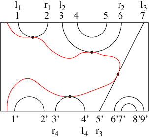
Consider $(p,s)\in{{\mathsf{J}}^{\bullet}}(m,n)$ , as in §2.4. See Fig.16(a) for a picture $d$ of an example, with $d\in[p]^{\prime}$ . (Note that here such pictures are unique up to ambient isotopy.) We can use such a picture $d$ of $(p,s)$ to describe a modification $\Psi(p,s)\in J^{1}_{0}(m+1,n+1)$ with the following steps:
(1) taking $d\in[p]^{\prime}$ , add new boundary points $0,0^{\prime}$ and draw a path between them that touches the lines of $d$ only at each of the blobs, as in Fig.16(b).
(2) noting that each blob now has four line segments incident, replace this with two crossing lines as in Fig.17, to obtain $d^{\prime}$ (Fig.16(c)).
(3) Set $\Psi(p,s)=\pi(d^{\prime})$ .

Note that (1) is possible by the left-exposed property of blobs.

(4.1) Lemma.

(I) The procedure $\Psi$ gives a map

\Psi:{{\mathsf{J}}^{\bullet}}(m,n)\to J^{1}_{0}(m+1,n+1)

(II) $\Psi$ is a bijection.
(III) For $(p,s)\in{{\mathsf{J}}^{\bullet}}(m,n)$ , writing $s=\{\{l_{1},r_{1}\},\{l_{2},r_{2}\},...\}$ where $l_{k}<r_{k}$ and this is the $k$ -th pair, both orderings with respect to the disk-order, then

\Psi(p,s)={\mathsf{x}}(s)\cup(p\setminus s)^{+}

where

{\mathsf{x}}(s)=\{\{1,r_{1}+1\},\{l_{1}+1,r_{2}+1\},\dots\{l_{|s|-1}+1,r_{s}+1\},\{l_{|s|},1^{\prime}\}\}

(IV) The map $\bar{\Psi}:J^{1}_{0}(m+1,n+1)\to{{\mathsf{J}}^{\bullet}}(m,n)$ given by $x\cup p\mapsto\bar{x}\cup p^{-}$ is inverse to $\Psi$ .
(V) If $\Psi(X)=Y\otimes u$ then $X$ takes the form $X=X^{\prime}\otimes u$ (in the obvious sense). ∎

Proof.

(I) It will be clear that the procedure gives an element of $J^{1}_{0}(m+1,n+1)$ . Thus it remains to show that this is independent of the choice of $d\in[p]^{\prime}$ representing $(p,s)\in{{\mathsf{J}}^{\bullet}}(m,n)$ . This follows since the construction of picture $d^{\prime}$ in $\Psi$ , both in the choice of $d$ and at steps (1-2), is unique up to ambient isotopy and produces a canonical picture. (It also follows that we can recast the procedure at the original set-theoretic level. See (III).)

(II) Note also that steps (1) and (2) are reversible. By (3.2) we can pass from $p\in J^{1}_{0}(m+1,n+1)$ to a canonical picture. Thus $\Psi$ is invertible.

(III) This is the promised formal version of the picture manipulation. Confer Lemma 3.13, (6) and Fig.17.

(IV) This is a disjoint combination of manifest inverses.

(V) Follows from (IV). ∎

4.2 An algebra isomorphism

(4.2) There is a map $\Theta$ on the ${\mathfrak{b}}_{n}$ generator set $U^{e}$ (cf. Theorem 2.26) to $kJ_{0}^{1}(n+1,n+1)$ given by:

U_{i}\mapsto U_{i+1}\;=\Psi(U_{i}),\qquad\qquad e\mapsto\frac{1}{2}(1+\sigma_{1})\;=\frac{1}{2}(\Psi(1)+\Psi(e))

(7)

(note the uses of notation $U_{i}$ distinguished by context).

(4.3) Theorem.

Fix a commutative ring $k$ and $\delta\in k$ , and set $\delta^{\prime}=\frac{\delta+1}{2}$ . Map $\Theta$ extends to an algebra isomorphism $\Theta:{\mathfrak{b}}_{n}\rightarrow{J}^{1}_{0,n+1}$ (with ${J}^{1}_{0,n+1}$ as defined in §3.5).

Proof.

To verify that $\Theta$ extends to an algebra homomorphism it is enough, by Theorem 2.26, to check that the images obey the relations $\tau^{\prime}$ from that Theorem. The relations on the $\{U_{i}\}$ are all clear. The image of $ee=e$ is clear. Next $U_{1}eU_{1}=\delta^{\prime}U_{1}$ :

U_{2}\frac{1}{2}(1+\sigma_{1})U_{2}=\frac{\delta+1}{2}U_{2}

The remaining commutation relations will be clear.

This homomorphism is surjective on $B_{2,2,n+1}$ since it hits the generators. On the other hand $B_{2,2,n+1}=J_{0,n+1}^{1}$ by Theorem 3.25. But ${\mathfrak{b}}_{n}$ and $J_{0,n+1}^{1}$ are isomorphic as vector spaces by Lem.4.1. ∎

4.3 Category version

(4.4) For $m,n\in\mathbb{N}_{0}$ define

	$\displaystyle\Phi:{{\mathsf{J}}^{\bullet}}(m,n)$	$\displaystyle\to$	$\displaystyle k{J}_{0}^{1}{}(m+1,n+1)$
	$\displaystyle(p,s)$	$\displaystyle\mapsto$	$\displaystyle 2^{-\|s\|}\sum_{z\subseteq s}\Psi(p,z)$

and extend $k$ -linearly. We write $\Phi_{m,n}$ to indicate cases of $\Phi$ where convenient.

(4.5) Recall (Thm.2.26(II)) that every (blob-)partition $(p,s)$ can be expressed as a product of generators, and write $\#(p,s)$ for the length (the minimum number of factors in such a word).
Remark: it is not in general easy to determine length from $(p,s)$ itself. It is easy to determine the number of factors $e$ , since this is just $|s|$ . Note also that disk order induces a total order on $s$ . For example if $\{a,b\}$ is the last pair in $s$ with $a<b$ in disk order then the image under $\Psi$ includes $\{a+1,1^{\prime}\}$ .

(4.6) Lemma.

The map $\Phi$ restricts to an algebra isomorphism ${\mathfrak{b}}_{n}(\delta,(\delta+1)/2)\rightarrow J_{0,n+1}^{1}$ . That is, $\Phi=\Theta$ when $m=n$ .

Proof: We work by induction on word length, as in (4.3). The base case is trivial.

Consider $(p,s)$ with $|s|=j>0$ and consider the same partition with one fewer blobs, $(p,s\setminus a)$ say (here $a$ is one of the pairs in $s$ ). Then

\Phi(p,s)=\frac{1}{2^{|s|}}\left(\sum_{z\subseteq s\setminus a}\Psi(p,z)+\sum_{z\subseteq s\setminus a}\Psi(p,z\cup\{a\})\right)

(8)

We assume $\Phi(w)=\Theta(w)$ for words $w$ of length $\leq l$ , and aim to show for words of length $l+1$ . Every such word may be written in the form $wx$ where $w$ has length $l$ and $x$ is a generator. First consider $x=e$ . If $(p,s)=we$ in ${\mathfrak{b}}_{n}$ then $s$ has an element $a=\{1^{\prime},j\}$ for some $j$ , and $w=(p,s\setminus a)$ . Note that in this case $\Psi(p,z\cup\{a\})=\Psi(p,z)\Psi(e)$ . So in this case (8) becomes

\Phi(p,s)=\frac{1}{2}\left(\Phi(p,s\setminus a)+\sum_{z\subseteq s\setminus a}\Psi(p,z)\Psi(e)\right)=\Phi(p,s\setminus a)\frac{1}{2}\left(\Psi(1)+\Psi(e)\right)=\Phi(p,s\setminus a)\Theta(e)

by (7). By inductive assumption, $\Phi(w)=\Theta(w)$ , so we have made the inductive step in this case.

Similarly if $(p,s)=wU_{i}$ for some $i$ , with $wU_{i}$ longer than $w=(p_{w},s_{w})$ , then either $w\mapsto wU_{i}$ does not change $s$ , $p=p_{w}U_{i}$ and

\Phi(p,s)=\frac{1}{2^{|s|}}\sum_{z\subseteq s}\Psi(p,z)=\frac{1}{2^{|s|}}\sum_{z\subseteq s}\Psi(p_{w}U_{i},z)=\frac{1}{2^{|s|}}\sum_{z\subseteq s}\Psi(p_{w},z)\Psi(U_{i})=\Phi(p_{w},s)\Theta(U_{i})

or $w\mapsto wU_{i}$ changes a single element of $s$ by $\{i^{\prime},j\}\mapsto\{k,j\}$ (where $k$ is the element in a pair with $i+1^{\prime}$ in $p_{w}$ ) and similarly $\Psi(p,s)=\Psi(p_{w},s_{w})\Theta(U_{i})$ . This completes the inductive step. ∎

(4.7) Lemma.

Let $(p,s)\in J^{\bullet}(m,n)$ and $p_{0}\in J_{-1}(m_{0},n_{0})$ . Then we have the following (confer (2.17) and (2.11)).
(i) the operation $(p,s)\mapsto(p\otimes p_{0},s)$ defines an injection $f_{-\otimes p_{0}}:J^{\bullet}(m,n)\hookrightarrow J^{\bullet}(m+m_{0},n+n_{0})$ , and similarly on the corresponding vector spaces.
(ii)

\Phi_{m+m_{0},n+n_{0}}(p\otimes p_{0},s)=\Phi_{m,n}(p,s)\otimes p_{0}.

(9)

Proof.

(i) $(p\otimes p_{0},s)\in J^{\bullet}(m+m_{0},n+n_{0})$ since the height of a picture is not increased by concatenating a non-crossing piece to the right and $s\subseteq S_{p}^{L}$ implies $s\subseteq S_{p\otimes p_{0}}^{L}$ . Injectivity is clear. (ii) Now

\Phi(p\otimes p_{0},s)=2^{-|s|}\sum_{z\subseteq s}\Psi(p\otimes p_{0},z)=2^{-|s|}\sum_{z\subseteq s}\Psi(p,z)\otimes p_{0}=\Phi(p,s)\otimes p_{0}\ ,

(10)

where the second equality holds by construction since the $p_{0}$ part has no blobs. ∎

(4.8) Theorem.

The collection of maps $\Phi=\Phi_{m,n}$ yields an equivalence between category ${\mathfrak{b}}$ (with $\delta^{\prime}=(1+\delta)/2$ ) and category ${\cal J}^{1}_{0}$ (the map on objects is $\Phi(n)=n+1$ ).

Proof. It is enough to show:
(1) Map $\Phi$ is a $k$ -vector space isomorphism $\Phi:k{{\mathsf{J}}^{\bullet}}(m,n)\rightarrow k{J}_{0}^{1}(m+1,n+1)$ .
(2) For any $(p,s)\in{{\mathsf{J}}^{\bullet}}(m,n)$ and $(p^{\prime},s^{\prime})\in{{\mathsf{J}}^{\bullet}}(n,q)$ then $\Phi(p,s)*\Phi(p^{\prime},s^{\prime})=\Phi((p,s)\circ(p^{\prime},s^{\prime})).$

For (1) consider first a case with $m<n$ . By construction there exists $x$ such that $n-m=2x$ . Then $p_{0}=u^{\otimes x}$ in (4.7) gives an embedding into the rank $n$ ‘algebra’ case. Now suppose (for a contradiction) that $\Phi$ is not injective. By (4.7) this would induce non-injectivity in the algebra case, contradicting (4.6).

For surjectivity we may proceed as follows. Suppose $X$ lies in $kJ^{1}_{0}(m-1,m+1)$ . Then $X\otimes u\in J^{1}_{0}(m+1,m+1)=J^{1}_{0,m}$ and so by Lemma 4.6 there exists $Y\in b_{m}$ such that $\Phi(Y)=X\otimes u$ . From Lemma 4.1(V) and the construction we see that $Y=Y^{\prime}\otimes u$ and $\Phi(Y^{\prime})=X$ . Thus $\Phi$ is surjective in this case. Other cases are similar.

For (2) let $t=\max(m,n,q)$ . For any $p_{0}\in J_{-1}(t-m,t-n)$ and $p_{0}^{\prime}\in J_{-1}(t-n,t-q)$ note that $(p\otimes p_{0},s),\;(p^{\prime}\otimes p_{0}^{\prime},s^{\prime})\;\in\;J^{\bullet}(t,t)$ . Since $\Phi=\Theta$ is an algebra isomorphism we have

\Phi((p\otimes p_{0},s)\circ(p^{\prime}\otimes p_{0}^{\prime},s^{\prime}))=\Phi(p\otimes p_{0},s)*\Phi(p^{\prime}\otimes p^{\prime}_{0},s^{\prime})\ .

(11)

Let us expand the left-hand side first. By construction

(p\otimes p_{0},s)\circ(p^{\prime}\otimes p_{0}^{\prime},s^{\prime})=((p,s)\circ(p^{\prime},s^{\prime}))\otimes(p_{0}*p_{0}^{\prime})

hence, using Lemma 4.7, we have

\Phi((p\otimes p_{0},s)\circ(p^{\prime}\otimes p_{0}^{\prime},s^{\prime}))=\Phi((p,s)\circ(p^{\prime},s^{\prime}))\otimes(p_{0}*p_{0}^{\prime})\ .

(12)

Now, the r.h.s. of (11) using Lemma 4.7 for both terms reads

\Phi(p\otimes p_{0},s)*\Phi(p^{\prime}\otimes p^{\prime}_{0},s^{\prime})=(\Phi(p,s)\otimes p_{0})*(\Phi(p^{\prime},s^{\prime})\otimes p_{0}^{\prime})=(\Phi(p,s)*\Phi(p^{\prime},s^{\prime}))\otimes(p_{0}*p^{\prime}_{0})\ ,

(13)

where the right equality holds by construction. The statement (2) of the lemma follows from the equality of the r.h.s. of (12) and (13) by Lemma 2.13(II). ∎

5 On representation theory consequences for short Brauer algebras

5.1 Summary of relevant results for ${\mathfrak{b}}_{n}$

Let us restrict to the case $k=\mathbb{C}$ . From a representation theory perspective the natural parameterisation of ${\mathfrak{b}}_{n}$ is $\delta=[2]$ (recall $[n]=(q^{n}-q^{-n})/(q-q^{-1})$ ) and $\delta^{\prime}=\frac{[m+1]}{[m]}$ . Then if $m\not\in\mathbb{Z}$ we know that ${\mathfrak{b}}_{n}$ is semisimple, with a well-known structure [22]. If $m\in\mathbb{Z}$ but $q$ not a root of unity then the algebras are no longer semisimple (for sufficiently large $n$ ), but the structure is still relatively simple to describe. The most interesting case is $m\in\mathbb{Z}$ and $q$ a root of unity. The structure in this case is quite complicated. See e.g. [9] for a full description. With this summary in mind, note that due to (4.3) we are interested in the cases when

\frac{[m+1]}{[m]}\;=\;\frac{[2]+1}{2}

This is solved for example by $m=1$ when $[2]=1$ .

For our present purposes the key point here has a precursor already even from the arithmetically simpler Temperley–Lieb case, as follows.

(5.1) Recall (see e.g. [19]) that the Chebyshev polynomials are the polynomials $d_{n}$ determined by the recurrence $d_{n+2}=xd_{n+1}-d_{n}$ , with initial conditions $d_{0}=1,d_{1}=x$ . (We write $x$ for $\delta$ here, simply for reasons of familiarity.) The first few are $d_{n}=1,x,x^{2}-1,x^{3}-2x,x^{4}-3x^{2}+1,...$ ( $n=0,1,2,3,...$ ).

These arise for example as the determinants of gram matrices such as:

\Delta^{n}_{n-2}=\left(\begin{array}[]{cccccccc}\delta&1&0&0&0\\ 1&\delta&1&0&0\\ 0&1&\delta&1&0\\ 0&0&1&\delta&1\\ 0&0&0&1&\delta\end{array}\right)

The obvious translational symmetry of this structure (arising from the local geometrical translational symmetry - the monoidal structure - of the TL diagram ‘particles’) gives rise to the natural fourier parameterisation $d_{n-1}=[n]$ . Loosely speaking, the geometrical boundary conditions here pick out a pure fourier sine series (fixing one end); and then the $n$ value (fixing the other end — hence the special behaviour at roots of unity of $q$ ). The blob algebra generalises this essentially by changing the boundary conditions. Next we look for evidence of similar phenomena in the short Brauer case.

5.2 Gram matrices, towers of recollement

We assume familiarity with the representation theory as treated in [14], including the construction of standard modules.

Here we restrict consideration to height 0. Our labeling scheme for Gram matrices $\Delta^{n}_{\lambda}$ of the standard modules ${\mathcal{S}}^{n}_{\lambda}$ is $\Delta^{n}_{\lambda}=\Delta^{n}_{m,\pm}$ (superscript: algebra rank $n$ ; subscript: number $m$ of propagating lines and (for $m>1$ ) $\pm$ is the symmetric / antisymmetric label from $S_{2}$ ). See Fig.18. For example, the diagram basis for the $n=6$ standard module corresponding to $\lambda=(4,+)$ can be drawn as:

where we omit to draw the $(2)$ -symmetrizer sitting on the first two propagating lines (thus we can draw the $\lambda=(4,-)$ case similarly, provided we keep in mind the omission, which affects calculations). Note that the basis (so drawn) contains one extra diagram compared to the $l=-1$ /Temperley–Lieb case.

The extra diagram has an interesting effect on the gram matrix of the natural contravariant form (see [14]). As for the TL case this can be computed in terms of Chebyshev polynomials (or equivalently fourier transforms). But here the initial conditions are different. We have

\Delta^{3}_{1}=\left(\begin{array}[]{cccccccc}\delta&1&1\\ 1&\delta&1\\ 1&1&\delta\end{array}\right),\hskip 25.36661pt\Delta^{4}_{2,\pm}=\left(\begin{array}[]{cccccccc}\delta&1&1&0\\ 1&\delta&1&\pm 1\\ 1&1&\delta&1\\ 0&\pm 1&1&\delta\end{array}\right),\hskip 25.36661pt\Delta^{n}_{n-2,+}=\left(\begin{array}[]{cccccccc}\delta&1&1&0&0&0\\ 1&\delta&1&1&0&0\\ 1&1&\delta&1&0&0\\ 0&1&1&\delta&1&0\\ 0&0&0&1&\delta&1\\ 0&0&0&0&1&\delta\end{array}\right)

(we give the $n=6$ example, but the general pattern will be clear). Laplace explanding $D^{n}_{\lambda}=|\Delta^{n}_{\lambda}|$ with respect to the bottom row we get a Chebyshev recurrence

D^{n}_{n-2,\pm}=\delta D^{n-1}_{n-3,\pm}-D^{n-2}_{n-4,\pm}

where the initial conditions are $D^{3}_{1}=(\delta-1)^{2}(\delta+2)$ and $D^{4}_{2,+}=\delta(\delta-1)(\delta^{2}+\delta-4)$ and $D^{4}_{2,-}=(\delta-1)(\delta+1)(\delta-2)(\delta+2)$ .

Note from Theorem 1.1(ii) of [10] (the tower-of-recollement method) and Proposition 5.3 of [14] (standard restriction rules) that the other gram determinants and indeed the ‘reductive’ representation theory can be determined from this subset of gram determinants. We will address this task in a separate paper. Here we restrict to some of the key preliminary observations.

The Chebyshev polynomials $d_{n}$ from (5.1) are a basis for the space of polynomials; and the recurrence is linear, so we can express our recurrence in terms of them, and hence make use of their more ‘fourier-like’ formulations: $d_{n-1}=[n]=\frac{q^{n}-q^{-n}}{q-q^{-1}}$ , where $\delta=x=q+q^{-1}$ . The determinants $D_{n}^{\pm}$ of the key subset of Gram matrices of form $\Delta^{n}_{n-2,\pm}$ can be expressed as

	$\displaystyle D_{n}^{+}$	$\displaystyle=$	$\displaystyle(x-1)\left[(x+2)(x-1)d_{n-3}-2xd_{n-4}\right]$		(14)
	$\displaystyle D_{n}^{-}$	$\displaystyle=$	$\displaystyle(x-1)(x+2)\left[(x-1)d_{n-3}-2d_{n-4}\right]$		(15)

Explicitly, the low rank cases of all the Gram matrices are as follows:

$\displaystyle D_{1}^{3}$	$\displaystyle=$	$\displaystyle(x-1)^{2}(x+2)$
$\displaystyle D_{0}^{4}$	$\displaystyle=$	$\displaystyle(x-1)^{2}x^{3}(x+2)$
$\displaystyle D_{2}^{4+}$	$\displaystyle=$	$\displaystyle(x-1)x(x^{2}+x-4)$
$\displaystyle D_{2}^{4-}$	$\displaystyle=$	$\displaystyle(x-1)(x+1)(x-2)(x+2)$
$\displaystyle D^{5}_{1}$	$\displaystyle=$	$\displaystyle(x-1)^{12}(x+1)(x-2)(x+2){{}^{6}(x^{2}+x-4)}$
$\displaystyle D^{5+}_{3}$	$\displaystyle=$	$\displaystyle(x-1)(x^{4}+x^{3}-5x^{2}-x+2)$
$\displaystyle D^{5-}_{3}$	$\displaystyle=$	$\displaystyle(x-1)(x+2)(x^{3}-x^{2}-3x+1)$
$\displaystyle D^{6}_{0}$	$\displaystyle=$	$\displaystyle(x-1)^{12}x^{11}(x+1)(x-2)(x+2)^{6}(x^{2}+x-4)$
$\displaystyle D^{6+}_{2}$	$\displaystyle=$	$\displaystyle(x-1)^{8}x^{5}(x+1)(x-2)(x+2)(x^{2}+x-4)^{6}(x^{4}+x^{3}-5x^{2}-x+2)$
$\displaystyle D^{6-}_{2}$	$\displaystyle=$	$\displaystyle(x-1)^{8}(x+1)^{6}(x-2)^{6}(x+2)^{7}(x^{2}+x-4)(x^{3}-x^{2}-3x+1)$
$\displaystyle D^{6+}_{4}$	$\displaystyle=$	$\displaystyle(x-1)^{2}x(x^{3}+2x^{2}-4x-6)$
$\displaystyle D^{6-}_{4}$	$\displaystyle=$	$\displaystyle(x-1)^{2}(x+2)(x^{3}-4x-2)$

(the cases not computed by recursion may be computed by brute force, see below).

A key point to take from this is that the short Brauer algebras manifest some similarities with the root-of-unity paradigm for non-semisimplicity, but move beyond it. As noted, taken in combination with tower of recollement methods these results ‘seed’ the reductive representation theory (the determination of decomposition matrices). We address this analysis fully in a separate paper, but the programme may be illustrated as follows.

This form corresponds to the map from the standard module ${\mathcal{S}}^{n}_{\lambda}$ to its contravariant dual which, on general grounds, maps the simple head to the socle [14]. Thus when the form is non-singular we deduce that the standard module is simple. And on the other hand when it is singular the standard module will have a corresponding submodule. It is not generally easy to determine the rank of the form and hence the dimension of the simple head from the gram determinant. For example the rank of $\Delta^{5}_{1}$ is easily seen to be 1, while the dimension of ${\mathcal{S}}^{5}_{1}$ is 11 (see Fig.18 or below) and the determinant factor is $(x-1)^{12}$ .

To illustrate first consider $D^{3}_{1}$ . The basis here is $\{\includegraphics[width]{xfig/S31a.eps},\includegraphics[width]{xfig/S31bb.eps},\includegraphics[width]{xfig/S31c.eps}\}$ . For example the action of generators on the element $\includegraphics[width]{xfig/S31bb.eps}-\includegraphics[width]{xfig/S31a.eps}$ at the singular point $\delta=x=1$ is:

\stackrel{{\scriptstyle\includegraphics[width]{xfig/S31d.eps}}}{{\includegraphics[width]{xfig/S31bb.eps}}}-\stackrel{{\scriptstyle\includegraphics[width]{xfig/S31d.eps}}}{{\includegraphics[width]{xfig/S31a.eps}}}\quad=\;0,\mbox{ }\quad\quad\stackrel{{\scriptstyle\includegraphics[width]{xfig/S31e.eps}}}{{\includegraphics[width]{xfig/S31bb.eps}}}-\stackrel{{\scriptstyle\includegraphics[width]{xfig/S31e.eps}}}{{\includegraphics[width]{xfig/S31a.eps}}}\quad=\;0,\mbox{ and }\quad\stackrel{{\scriptstyle\includegraphics[width]{xfig/S31ff.eps}}}{{\includegraphics[width]{xfig/S31bb.eps}}}-\stackrel{{\scriptstyle\includegraphics[width]{xfig/S31ff.eps}}}{{\includegraphics[width]{xfig/S31a.eps}}}\quad=\;-(\includegraphics[width]{xfig/S31bb.eps}-\includegraphics[width]{xfig/S31a.eps})

That is, when $\delta=x=1$ this element spans a submodule isomorphic to ${\mathcal{S}}^{3}_{3,-}$ . Meanwhile for the element $\includegraphics[width]{xfig/S31a.eps}+\includegraphics[width]{xfig/S31bb.eps}-2\includegraphics[width]{xfig/S31c.eps}$ :

\stackrel{{\scriptstyle\includegraphics[width]{xfig/S31d.eps}}}{{\includegraphics[width]{xfig/S31a.eps}}}+\stackrel{{\scriptstyle\includegraphics[width]{xfig/S31d.eps}}}{{\includegraphics[width]{xfig/S31bb.eps}}}-2\stackrel{{\scriptstyle\includegraphics[width]{xfig/S31d.eps}}}{{\includegraphics[width]{xfig/S31c.eps}}}\quad=\quad\stackrel{{\scriptstyle\includegraphics[width]{xfig/S31e.eps}}}{{\includegraphics[width]{xfig/S31a.eps}}}+\stackrel{{\scriptstyle\includegraphics[width]{xfig/S31e.eps}}}{{\includegraphics[width]{xfig/S31bb.eps}}}-2\stackrel{{\scriptstyle\includegraphics[width]{xfig/S31e.eps}}}{{\includegraphics[width]{xfig/S31c.eps}}}\quad=\;0,

\stackrel{{\scriptstyle\includegraphics[width]{xfig/S31ff.eps}}}{{\includegraphics[width]{xfig/S31a.eps}}}+\stackrel{{\scriptstyle\includegraphics[width]{xfig/S31ff.eps}}}{{\includegraphics[width]{xfig/S31bb.eps}}}-2\stackrel{{\scriptstyle\includegraphics[width]{xfig/S31ff.eps}}}{{\includegraphics[width]{xfig/S31c.eps}}}\quad=\;\includegraphics[width]{xfig/S31a.eps}+\includegraphics[width]{xfig/S31bb.eps}-2\includegraphics[width]{xfig/S31c.eps}

So this element spans a submodule isomorphic to ${\mathcal{S}}^{3}_{3,+}$ . We deduce that the simple head is one-dimensional.

On the other hand consider $\includegraphics[width]{xfig/S31a.eps}+\includegraphics[width]{xfig/S31bb.eps}+\includegraphics[width]{xfig/S31c.eps}$ in case $\delta=x=-2$ . This spans a submodule isomorphic to ${\mathcal{S}}^{3}_{3,+}$ . Here the simple head is two-dimensional.

By the module-category embedding property [14, (4.26)] these standard module morphisms have images in higher ranks, thus when $x=1$ our map ${\mathcal{S}}^{3}_{3,-}\rightarrow{\mathcal{S}}^{3}_{1}$ gives a map ${\mathcal{S}}^{5}_{3,-}\rightarrow{\mathcal{S}}^{5}_{1}$ and so on. The embedding functor is not exact so we cannot tell directly from the gram matrix if an image map has a kernel. So (comparing also with the dimensions from Fig.18), a naive lower bound on the exponent in the factor $(x-1)^{12}$ in $D^{5}_{1}$ is 4+4, corresponding to the dimensions of the simple heads of ${\mathcal{S}}^{5}_{3,+}$ and ${\mathcal{S}}^{5}_{3,-}$ when $x=1$ . It is intriguing to compare with the blob case [9]. There the embedded standard module morphisms are injective, but if that is the case here the naive bound is still only lifted to 5+5, so we see that there will be some nice subtleties here.

As a further illustration, the basis for $n=6$ and $\lambda=0$ is:

(N.B. the basis for $n=5$ , $\lambda=1$ is combinatorially identical). (As noted, we do not strictly need such cases for the ‘Cox criterion’. It is enough to use $\lambda=n-2$ . We include it for curiosity’s sake.) The corresponding gram matrix then comes from the array in Fig.19.

Thus, writing $j$ for $\delta^{j}$ (with $j$ the number of connected components in a diagram), the gram matrix is given by

\left(\begin{array}[]{ccccc|ccccc|cc}3&2&2&1&2&2&1&2&1&2&1\\ 2&3&1&2&1&1&2&1&1&2&1\\ 2&1&3&2&1&2&1&1&2&1&1\\ 1&2&2&3&2&1&2&1&2&1&1\\ 2&1&1&2&3&1&1&2&1&1&2\\ \hline\cr 2&1&2&1&1&3&2&1&1&1&2\\ 1&2&1&2&1&2&3&2&1&1&2\\ 2&1&1&1&2&1&2&3&2&1&1\\ 1&1&2&2&1&1&1&2&3&2&2\\ 2&2&1&1&1&1&1&1&2&3&2\\ \hline\cr 1&1&1&1&2&2&2&1&2&2&3\end{array}\right)

The determinant here can still be computed by brute force.

6 Discussion

Some notable open questions follow.

Q1. How to generalise the ‘short Brauer’ construction to the BMW algebra [3, 25]?

Q2. How to relate the usual two-parameter version of the blob algebra to the short Brauer algebras — which by the original construction have only a single parameter.

Recall that there is, essentially trivially, a two-parameter version of $T_{n}$ . First recall that $T_{n}$ has a basis of non-crossing Brauer diagrams [32, 7] up to ambient isotopy (see §2 for a summary of Brauer diagram concepts — ambient isotopy does not include, for example, the Reidemeister moves included in general Brauer diagram equivalence, but it is sufficient in the non-crossing case, and this is key here). The elements of the basis can be seen as partitioning the interval into alcoves. These alcoves can be shaded black or white with the property that
(A1) the colour changes across each boundary; and
(A2) the leftmost alcove is white, say.
(NB Another way of saying this is that arcs have a well-defined ‘height’ in the sense of this paper, which is either odd or even.)
Thus in composition both black and white loops may form. The number of each separately is an invariant of ambient isotopy. It follows that we may associate a different parameter to each.

Thus we have an algebra $T_{n}(\delta_{b},\delta_{w})$ , say. It is easy to see that $T_{n}(\delta_{b},\delta_{w})\cong T_{n}(\alpha\delta_{b},\delta_{w}/\alpha)$ for any unit $\alpha$ , so the difference can usually be scaled away. For example recall the following.

(6.1) Theorem.

[19] Consider the algebra defined by generators $U=\{U_{1},U_{2},...,U_{n-1}\}$ and relations $\tau=\{\mbox{ $U_{i}^{2}=\delta U_{i}$, $U_{i}U_{i\pm 1}U_{i}=U_{i}$, $U_{i}U_{j}=U_{j}U_{i}$, $j\neq i\pm 1$ }\}$ . The map

U_{i}\mapsto u_{i}=\{\{1,1^{\prime}\}\{2,2^{\prime}\},...,\{i,i+1\},\{i^{\prime},i+1^{\prime}\},...,\{n,n^{\prime}\}\}\qquad(i=1,2,...,n-1)

extends to an algeba isomorphism $k\langle U\rangle/\tau\cong T_{n}$ . ∎

To see the isomorphic two-parameter version consider the effect on the relations of the map $U_{i}\mapsto\alpha U_{i}$ ( $i$ odd), $U_{i}\mapsto\alpha^{-1}U_{i}$ ( $i$ even).

The blob algebra ${\mathfrak{b}}_{n}$ can be seen as the subalgebra of $T_{2n}(\delta_{b},\delta_{w})$ generated by diagrams with a lateral-flip symmetry. In this subalgebra, however, it is not possible to scale away the second parameter.

The short Brauer algebras are, from one perspective, generalisations of $T_{n}$ . It is interesting to consider if there are analogous generalisations of the two-parameter version that (like the blob) have the property that the second parameter becomes material. This is not obvious. The generalisation destroys the two-tone alcove construction.

How does the two-tone construction look in the categorical setting? Here we write $T(n,m)$ for the subset $J_{-1}(n,m)$ of $J(n,m)$ of non-crossing pair-partitions. We fix $\delta\in k$ and note that ${\mathcal{T}}=(\mathbb{N}_{0},kT(n,m),*)$ is a subcategory of ${\mathcal{B}}$ . Indeed ${\mathcal{T}}={\mathcal{B}}^{-1}$ . The inclusion is of $k$ -linear categories, and also of monoidal $k$ -linear categories.

As in the algebra case we note that in the non-crossing setting we can count the number of black and white loops separately (i.e. these numbers are separately well-defined). Note however that the monoidal structure on ${\mathcal{T}}$ does not preserve this property. It is the axiom (A2) that is the problem.

Acknowledgements. We thank EPSRC for funding under grant EP/I038683/1. We thank Shona Yu, Azat Gaynutdinov and Peter Finch for useful conversations.

Appendix

Appendix A Colour pictures for Lemma 3.24

Consider Lemma 3.24. When $j<i$ , the initial points of chain from $i$ and $i+1$ are interchanged (see Fig. 20a)). When $j=i$ we have three different cases: (i) The line from $i+1$ is part of a chain from $[1,i]$ , distinct from that from $i$ , (ii) both lines from $i$ and $i+1$ belong to the same chain, (iii) the line from $(i+1)$ is non intersecting. Observe from Fig. 20b),c),d) that the resulting partitions are $Li-$ simple with $i$ exclusive chains from $[1,i]$ to $[1^{\prime},i^{\prime}]$ and standalone pairs with no intersecting region with any other pair of chains.

References

[1] F. C. Alcaraz, M. N. Barber, M. T. Batchelor, R. J. Baxter, and G. R. W. Quispel, Surface exponents of the quantum XXZ, Ashkin-Teller and Potts models, Journal of Physics A Mathematical General 20 (1987), 6397–6409.
[2] H H Andersen, J C Jantzen, and W Soergel, Representation of quantum groups at a $p^{th}$ root of unity and of semisimple groups in characteristic $p$ : independence of $p$ , Asterisque 220 (1994).
[3] J S Birman and H Wenzl, Braids, link polynomials and a new algebra, Transactions AMS 313 (1989), 249–273.
[4] Roberto Bondersan, private communication.
[5] C Bowman, A G Cox, and L Speyer, A family of graded decomposition numbers for diagrammatic Cherednik algebras, IMRN 2017 (2017), 2686.
[6] R Brauer, On algebras which are connected with the semi–simple continuous groups, Annals of Mathematics 38 (1937), 854–872.
[7] W P Brown, Michigan Math. J. 3 (1955-56), 1–22.
[8] A Cox and M De Visscher, Diagrammatic kazhdan-lusztig theory for the (walled) brauer algebra, J Alg 340 (2011).
[9] A G Cox, J J Graham, and P P Martin, The blob algebra in positive characteristic, J Algebra 266 (2003), 584–635.
[10] A G Cox, P P Martin, A E Parker, and C C Xi, Representation theory of towers of recollement: theory, notes and examples, J Algebra 302 (2006), 340–360, DOI 10.1016 online (math.RT/0411395).
[11] G. James and A. Kerber, The representation theory of the Symmetric group, Encyclopedia of Mathematics and its Applications, vol. 16, Addison-Wesley, 1981.
[12] G. D. James, The representation theory of the symmetric groups, Lecture Notes in Mathematics 682, Springer, 1978.
[13] A. Joyal and R. Street, Geometry of tensor calculus i, Advances in Mathematics 88 (1991), 55–113.
[14] Z Kadar, P P Martin, and S Yu, On geometrically defined extensions of the Temperley-Lieb category in the Brauer category, arXiv/1401.1774 (2014), Math.Z. (to appear).
[15] D Kazhdan and G Lusztig, Representations of coxeter groups and Hecke algebras, Inventiones Math. 53 (1979), 165–184.
[16] M. Khovanov and A. D. Lauda, A diagrammatic approach to categorification of quantum groups, Represent. Theory 13 (2009), 309–347.
[17] D Levy, Algebraic structure of translation-invariant spin-1/2 XXZ and q-Potts quantum chains, Phys Rev Lett 67 (1991), 1971–1974.
[18] E H Lieb and D C Mattis, Mathematical physics in one dimension, Academic Press, 1966.
[19] P P Martin, Potts models and related problems in statistical mechanics, World Scientific, Singapore, 1991.
[20] , Pascal’s triangle and a word basis for blob algebra ideals, arxiv:0706.1655 (2007).
[21] , The decomposition matrices of the Brauer algebra over the complex field, Trans. A.M.S. 367 (2015), 1797–1825, (http://arxiv.org/abs/0908.1500).
[22] P P Martin and H Saleur, The blob algebra and the periodic Temperley–Lieb algebra, Lett. Math. Phys. 30 (1994), 189–206, (hep-th/9302094).
[23] P P Martin and D Woodcock, Generalized blob algebras and alcove geometry, LMS J Comput Math 6 (2003), 249–296, (math.RT/0205263).
[24] E E Moise, Geometric topology in dimensions 2 and 3, Graduate Texts in Mathematics 47, Springer-Verlag, New York, 1977.
[25] J Murakami, The Kauffman polynomial of links and representation theory, Osaka J. Math. 24 (1987), no. 4, 745–758.
[26] V Ostrik, Module categories, https://arxiv.org/pdf/math/0111139.pdf (2001).
[27] V Pasquier and H Saleur, Common structures between finite systems and conformal field theories through quantum groups, Nucl Phys B 330 (1990), 523.
[28] R. Rouquier, 2-kac-moody algebras, arXiv:0812.5023 (2008).
[29] W. Soergel, Kazhdan-Lusztig polynomials and a combinatoric for tilting modules, Representation Theory 1 (1997), 83–114.
[30] W Soergel, Kazhdan-Lusztig-polynome und unzerlegbarebimoduln uber polynomringen, Journal of the Institute of Mathematics of Jussieu 6 (2007), 501–525.
[31] H N V Temperley and E H Lieb, Proceedings of the Royal Society A 322 (1971), 251–280.
[32] H Weyl, Classical groups, Princeton, Princeton, 1946.

Geometric partition categories: On short Brauer algebras and their blob subalgebras

1 Introduction

2 Preliminary definitions

2.1 Brauer picture calculus

2.2 The Brauer partition category ℬ{\mathcal{B}}

(2.11) Theorem.

Proof.

(2.13) Lemma.

2.3 The subcategory 𝒥l{\mathcal{J}}_{l} of category ℬ{\mathcal{B}}

(2.14) Theorem.

2.4 The blob category 𝔟{\mathfrak{b}}

(2.17) Lemma.

Proof.

(2.20) Theorem.

Proof.

(2.24.1) Corollary.

2.5 Generators and relations

(2.26) Theorem.

2.6 Generator algebras Bl,m,nB_{l,m,n} and spin chain Physics

3 The subcategory 𝒥i−1i{\mathcal{J}}_{i-1}^{i} of 𝒥i−1{\mathcal{J}}_{i-1}

3.1 The crossing number χp\chi_{p} of a partition

(3.4) Lemma.

Proof.

(3.5) Lemma.

Proof.

3.2 L​1L1-chain partitions

(3.13) Lemma.

Proof.

3.3 L​iLi-chain partitions

(3.23) Lemma.

Proof.

3.4 A Bi+1,i+1,mB_{i+1,i+1,m}-module of L​iLi-chain partitions

(3.24) Lemma.

Proof.

3.5 The Chain-basis Theorem

(3.25) Theorem.

Proof.

3.6 The category 𝒥l−1l{\mathcal{J}}_{l-1}^{l}

(3.26) Lemma.

Proof.

(3.27) Theorem.

Proof.

4 The blob isomorphism Theorem

4.1 The initial set map Ψ:𝖩∙​(m,n)→J01​(m+1,n+1)\Psi:{{\mathsf{J}}^{\bullet}}(m,n)\to J^{1}_{0}(m+1,n+1)

(4.1) Lemma.

Proof.

4.2 An algebra isomorphism

(4.3) Theorem.

Proof.

4.3 Category version

(4.6) Lemma.

(4.7) Lemma.

Proof.

(4.8) Theorem.

5 On representation theory consequences for short Brauer algebras

5.1 Summary of relevant results for 𝔟n{\mathfrak{b}}_{n}

5.2 Gram matrices, towers of recollement

6 Discussion

(6.1) Theorem.

Appendix

Appendix A Colour pictures for Lemma 3.24

References

Geometric partition categories:
On short Brauer algebras and their blob subalgebras

2.2 The Brauer partition category ${\mathcal{B}}$

2.3 The subcategory ${\mathcal{J}}_{l}$ of category ${\mathcal{B}}$

2.4 The blob category ${\mathfrak{b}}$

2.6 Generator algebras $B_{l,m,n}$ and spin chain Physics

3 The subcategory ${\mathcal{J}}_{i-1}^{i}$ of ${\mathcal{J}}_{i-1}$

3.1 The crossing number $\chi_{p}$ of a partition

3.2 $L1$ -chain partitions

3.3 $Li$ -chain partitions

3.4 A $B_{i+1,i+1,m}$ -module of $Li$ -chain partitions

3.6 The category ${\mathcal{J}}_{l-1}^{l}$

4.1 The initial set map $\Psi:{{\mathsf{J}}^{\bullet}}(m,n)\to J^{1}_{0}(m+1,n+1)$

5.1 Summary of relevant results for ${\mathfrak{b}}_{n}$