跳到论文正文
W Papers独立论文阅读器 arXiv:2002.05392 论文正文 计算阅读时间 · 0%
引用这篇论文根据当前论文元数据生成,正式投稿前建议核对。


License: arXiv.org perpetual non-exclusive license
arXiv:2002.05392v3 [cs.LG] 16 Jul 2020
\coltauthor

Faculty of Electrical Engineering, Technion, Israel Institute of Technology. and
Faculty of Electrical Engineering, Technion, Israel Institute of Technology.
Nvidia Research.

Tight Lower Bounds for Combinatorial Multi-Armed Bandits

Nadav Merlis Email: merlis@campus.technion.ac.il Affiliation:    Shie Mannor Email: shie@ee.technion.ac.il Affiliation: Affiliation:
Abstract

The Combinatorial Multi-Armed Bandit problem is a sequential decision-making problem in which an agent selects a set of arms at each round, observes feedback for each of these arms and aims to maximize a known reward function of the arms it chose. While previous work proved regret upper bounds in this setting for general reward functions, only a few works provided matching lower bounds, all for specific reward functions. In this work, we prove regret lower bounds for combinatorial bandits that hold under mild assumptions for all smooth reward functions. We derive both problem-dependent and problem-independent bounds and show that the recently proposed Gini-weighted smoothness parameter (Merlis and Mannor 2019) also determines the lower bounds for monotone reward functions. Notably, this implies that our lower bounds are tight up to log-factors.

keywords
Combinatorial Multi-Armed Bandits, Lower Bounds, Gini-Weighted Smoothness

1 Introduction

Combinatorial Multi-Armed Bandits (CMABs) are a well-known extension of Multi-Armed Bandits (MABs) (Robbins 1952), where instead of choosing a single arm at each round, the agent selects a set of arms. It then observes noisy feedback for each arm in this set (‘semi-bandit feedback’) and aims to maximize a known reward function of the selected arms and their parameters. More specifically, it aims to minimize its regret, which is the expected cumulative difference between the reward of the best action and the reward of the agent’s actions. The applications of this framework are numerous and vary between reward functions; the most common one is the linear reward function (Kveton et al. 2015c), which can be applied for problems such as spectrum allocation, shortest paths, routing problems and more (Gai et al. 2012). Another common application is the Probabilistic Maximum Coverage (PMC) problem (Merlis and Mannor 2019), which is closely related to problems such as influence maximization and ranked recommendations.

Due to its usefulness, many previous works analyze regret upper bounds for different variants of this setting. While some works focus on specific reward functions, others derive bounds that hold for general reward functions. In these cases, the bounds usually depend on some measure of smoothness of the reward, for example, its global Lipschitz constant, or its Gini-weighted smoothness. The latter is a more refined smoothness criterion, recently suggested in (Merlis and Mannor 2019), that takes into account the interaction between the local gradients of the reward and concentration properties of the arms. On the other hand, there are almost no works on matching lower bounds; to the best of our knowledge, all existing lower bounds for CMABs were derived for specific reward functions – either the linear one or the PMC problem. Notably, there is no characterization of lower bounds for general reward functions, and it is unclear whether existing upper bounds are tight.

The gain from general lower bounds is threefold: (i) When the bounds are loose, understanding which quantities affect the lower bounds allows devising tighter algorithms; (ii) When the bounds are tight, the instances on which the bounds were derived can help to determine under which additional assumptions the lower bounds do not hold. Such assumptions might allow us to derive improved upper bounds; (iii) When we can control some parameters of the problem, e.g., the number of arms in an action, their effect on the lower bound can help us tune them for each application.

In this work, we derive problem-dependent (Theorem 1) and problem-independent (Theorem 2) lower bounds that hold for general reward functions under mild assumptions. The problem-dependent bound shows that for any ‘good’ bandit strategy, there exists a CMAB instance such that the asymptotic regret must be larger than a certain logarithmic rate. The problem-independent bound shows that for any strategy and any large enough horizon TT, there exists a horizon-dependent instance with a T\sqrt{T} regret. To derive these bounds, we define a family of action sets for CMAB problems, which we call II-disjoint. There, a subset of arms II appear in all actions and independent of other actions, while the rest of the arms appear in a single action. We then prove that for II-disjoint problems, both bounds depend on a new modified Gini-smoothness measure; specifically, they reproduce existing lower bounds for both the linear reward function and the PMC problem. If the reward function is also monotone, as in most practical applications, we derive an additional bound that depends on the Gini-smoothness of the reward and matches the upper bound of (Merlis and Mannor 2019) up to logarithmic factors (Proposition 4). Thus, our results demonstrate that without any additional assumptions, the bounds are tight for almost any reward function.

2 Related Work

The general framework of combinatorial bandits with semi-bandit feedback was first presented in (Chen et al. 2013). Since then, it has had many extensions, e.g., for the case of probabilistically-triggered arms, where the set of arms in an action might be random (Chen et al. 2016a; Wang and Chen 2017), and for reward functions that depend on the arm distribution (Chen et al. 2016b). Moreover, many previous works focus on specific instances of this problem, e.g., linear reward functions (Kveton et al. 2015c; Combes et al. 2015; Degenne and Perchet 2016), cascading bandits (Kveton et al. 2015a; Kveton et al. 2015b) and more. Recently, Merlis and Mannor 2019 presented BC-UCB, a Bernstein-based UCB algorithm with regret bounds that depend on a new smoothness measure, which they call the Gini-weighted smoothness. Specifically, they show that by combining the reward nonlinearity with the local behavior of the confidence intervals, the dependency of previous regret bounds in the maximal action size can be removed. In this work, we show that for monotone reward functions, the Gini-smoothness also characterizes the lower bounds for CMAB problems and therefore prove that this upper bound is tight. In addition, while all previously stated papers assume that the reward function is monotone, a few papers also support non-monotone reward functions (Wang and Chen 2018; Hüyük and Tekin 2019). We also present lowers bounds for this scenario.

Although there has been extensive work on regret upper bounds for CMABs, there are almost no results on lower bounds for this setting. Kveton et al. 2015c derived lower bounds for the linear reward function with general arm distributions, and when arms are also independent, lower bounds can be found in (Degenne and Perchet 2016; Combes et al. 2015). Also, Kveton et al. 2015a derived lower bounds for cascading bandits and Merlis and Mannor 2019 derived bounds for the PMC problem. Nevertheless, and to the best of our knowledge, there are no lower bounds for general reward functions. A comparison of our bounds to previous related bounds can be found in Table 1.

In contrast to the CMAB problem, the lower bounds for MABs are well characterized. In their seminal work, Lai and Robbins 1985 presented the first general problem-dependent lower bound for MABs, which was later extended by Burnetas and Katehakis 1996. In terms of problem-independent bounds, Auer et al. 2002 derived an Ω⁡(K​T)\Omega(\sqrt{KT}) lower bound for KK-armed bandit problems with time horizon TT, whose constants were later improved by Cesa-Bianchi and Lugosi 2006. Also, Mannor and Tsitsiklis 2004 proved problem-independent lower bounds with both linear and logarithmic regimes. Recently, Garivier et al. 2018 presented a general tool that allows deriving various lower bounds for MABs. We adapt this tool for the CMAB problem to derive our new regret bounds.

Table 1: Upper (UB) and lower (LB) bounds of different CMAB problems for arbitrary action sets. Dep./Ind. are problem-dependent and problem-independent bounds, and the notations follow Section 3. γ∞\gamma_{\infty} is the global Lipschitz constant of a reward function, and for the Gini-smoothness γg\gamma_{g}, it holds that γg≤K​γ∞\gamma_{g}\!\leq\!\sqrt{K}\gamma_{\infty} (Merlis and Mannor 2019). Δmin\Delta_{\min} is the minimal gap.
CMAB problem Type Previous UB Previous LB Theorem 1 or 2 Proposition 4
General reward functions Dep. 𝒪​(γ∞2​m​K​ln⁡TΔmin)†\mathcal{O}\left(\frac{\gamma_{\infty}^{2}mK\ln T}{\Delta_{\min}}\right)^{\dagger} None Ω⁡(max𝝁,I⁡γ~g2​(𝝁,I)​m​ln⁡TΔmin​KI)\Omega\left(\max_{{\boldsymbol{\mu}},I}\frac{\tilde{\gamma}_{g}^{2}({\boldsymbol{\mu}};I)m\ln T}{\Delta_{\min}{K_{I}}}\right) NA
Ind. None None Ω⁡(max𝝁,I⁡γ~g2​(𝝁,I)​m​TKI)\Omega\left(\max_{{\boldsymbol{\mu}},I}\sqrt{\frac{\tilde{\gamma}_{g}^{2}({\boldsymbol{\mu}};I)mT}{{K_{I}}}}\right) NA
Monotone reward functions Dep. 𝒪​(γg2​m​ln2​K​ln⁡TΔmin)‡\mathcal{O}\left(\frac{\gamma_{g}^{2}m\ln^{2}K\ln T}{\Delta_{\min}}\right)^{\ddagger} None Ω⁡(max𝝁,I⁡γ~g2​(𝝁,I)​m​ln⁡TΔmin​KI)\Omega\left(\max_{{\boldsymbol{\mu}},I}\frac{\tilde{\gamma}_{g}^{2}({\boldsymbol{\mu}};I)m\ln T}{\Delta_{\min}{K_{I}}}\right) Ω~​(γg2​m​ln⁡TΔmin)\tilde{\Omega}\left(\frac{\gamma_{g}^{2}m\ln T}{\Delta_{\min}}\right)
Ind. 𝒪​(γg​ln⁡K​m​T)‡\mathcal{O}\left(\gamma_{g}\ln K\sqrt{mT}\right)^{\ddagger} None Ω⁡(max𝝁,I⁡γ~g2​(𝝁,I)​m​TKI)\Omega\left(\max_{{\boldsymbol{\mu}},I}\sqrt{\frac{\tilde{\gamma}_{g}^{2}({\boldsymbol{\mu}};I)mT}{{K_{I}}}}\right) Ω~​(γg​m​T)\tilde{\Omega}\left(\gamma_{g}\sqrt{mT}\right)
Linear reward function r(S; μ )=∑_i∈Sμ_i Dep. 𝒪​(m​K​ln⁡TΔmin)§\mathcal{O}\left(\frac{mK\ln T}{\Delta_{\min}}\right)^{\lx@sectionsign} Ω​(m​K​ln⁡TΔmin)§\Omega\left(\frac{mK\ln T}{\Delta_{\min}}\right)^{\lx@sectionsign} Ω⁡(m​K​ln⁡TΔmin)\Omega\left(\frac{mK\ln T}{\Delta_{\min}}\right) Ω⁡(m​K​ln⁡T(ln⁡K)​Δmin)\Omega\left(\frac{mK\ln T}{\left(\ln K\right)\Delta_{\min}}\right)
Ind. 𝒪​(m​K​T)§\mathcal{O}\left(\sqrt{mKT}\right)^{\lx@sectionsign} Ω​(m​K​T)§\Omega\left(\sqrt{mKT}\right)^{\lx@sectionsign} Ω⁡(m​K​T)\Omega\left(\sqrt{mKT}\right) Ω⁡(m​K​Tln⁡K)\Omega\left(\sqrt{\frac{mKT}{\ln K}}\right)
PMC problem r(S; μ )​=​∑_i=1^M​(​​1​-​∏_j∈S​(1-μ_ij)​​) Dep. 𝒪​(m​M2​ln2​K​ln⁡TΔmin)‡\mathcal{O}\left(\frac{mM^{2}\ln^{2}K\ln T}{\Delta_{\min}}\right)^{\ddagger} Ω​(m​M2​ln⁡TΔmin)‡\Omega\left(\frac{mM^{2}\ln T}{\Delta_{\min}}\right)^{\ddagger} Ω⁡(m​M2​ln⁡TΔmin)\Omega\left(\frac{mM^{2}\ln T}{\Delta_{\min}}\right) Ω⁡(m​M2​ln⁡T(ln⁡K)2​Δmin)\Omega\left(\frac{mM^{2}\ln T}{\left(\ln K\right)^{2}\Delta_{\min}}\right)
Ind. 𝒪​(M​ln⁡K​m​T)‡\mathcal{O}\left(M\ln K\sqrt{mT}\right)^{\ddagger} Ω​(M​m​T)‡\Omega\left(M\sqrt{mT}\right)^{\ddagger} Ω⁡(M​m​T)\Omega\left(M\sqrt{mT}\right) Ω⁡(M​m​Tln⁡K)\Omega\left(\frac{M\sqrt{mT}}{\ln K}\right)

3 Preliminaries and Notations

We start with some notations. Let [n]={1,…,n}[n]=\left\{1,\dots,n\right\}, and for any vector x∈ℝnx\!\in\!\mathbb{R}^{n} and set I⊂[n]I\!\subset\!\left[n\right], denote by xIx_{I}, a sub-vector of xx that contains only elements from II. We denote the Kullback-Leibler (KL) divergence between two distributions ν¯,ν¯′{\underline{\nu}},{\underline{\nu}}^{\prime} by DKL​(ν¯,ν¯′)D_{\mathrm{KL}}({\underline{\nu}},{\underline{\nu}}^{\prime}), and the KL divergence between two Bernoulli random variables with expectations p,qp,q by kl⁡(p,q)\mathrm{kl}(p,q). For any vector x∈ℝnx\!\in\!\mathbb{R}^{n}, let xsx^{s} be a permutation such that x1s≤…≤xnsx_{1}^{s}\!\leq\!\dots\!\leq\!x_{n}^{s}, and define the increasing permutation of vector x∈ℝnx\!\in\!\mathbb{R}^{n} w.r.t. a set II as px,I=[xIcs,xI]∈ℝnp^{x,I}\!=\!\left[x_{I^{c}}^{s},x_{I}\right]\!\in\!\mathbb{R}^{n}; namely, the beginning of the vector px,Ip^{x,I} contains a sorted permutation of the elements of xx in Ic=[n]/II^{c}=\left[n\right]/I, and its end contains the elements of xx in II. Finally, for any set II of bounded size |I|≤K\left\lvert I\right\rvert\leq K, we denote by KI=K−|I|{K_{I}}\!=\!K-\lvert I\rvert the size of the complementary set w.r.t. KK.

We work under the combinatorial multi-armed bandit setting with semi-bandit feedback. Denote the number of arms (‘base arms’) by mm, and let 𝒮⊂2[m]\mathcal{S}\subset 2^{\left[m\right]} be the set of possible actions (‘super arms’), that is, the set that contains all valid combinations of base arms that the agent can choose. The number of base arms in each action S∈𝒮S\in\mathcal{S} is bounded by |S|≤K\lvert S\rvert\leq K, and w.l.o.g., assume that |S|=K\lvert S\rvert=K. At the beginning of each round tt, the arms generate an observation vector X(t)=(X1(t),…,Xm(t))∈[0,1]mX^{(t)}\!=\!\left(X^{(t)}_{1},\dots,X^{(t)}_{m}\right)\in\left[0,1\right]^{m}, sampled from a fixed distribution independently of other rounds. Then, the agent chooses an action St∈𝒮S_{t}\in\mathcal{S} and observes feedback XS(t)≜{(i,Xi(t)),∀i∈St}X^{(t)}_{S}\triangleq\left\{\left(i,X^{(t)}_{i}\right),\forall i\in S_{t}\right\}. Denote the means of base arms by 𝔼⁡[X(t)]=𝝁=(μ1,…,μm)\mathbb{E}\left[X^{(t)}\right]\!=\!{\boldsymbol{\mu}}\!=\!\left(\mu_{1},\dots,\mu_{m}\right). The goal of the agent is to maximize a known reward function r⁡(S,𝝁)r\left(S;{\boldsymbol{\mu}}\right), without knowing 𝝁{\boldsymbol{\mu}}. Specifically, the agent aims to minimize its regret R⁡(T)=∑t=1T(r⁡(S∗,𝝁)−r⁡(St,𝝁))≜∑t=1TΔStR(T)=\sum_{t=1}^{T}\left(r\left(S^{*};{\boldsymbol{\mu}}\right)-r\left(S_{t};{\boldsymbol{\mu}}\right)\right)\triangleq\sum_{t=1}^{T}\Delta_{S_{t}}, where S∗∈arg⁡maxS∈𝒮⁡r​(S,𝝁)S^{*}\in\argmax_{S\in\mathcal{S}}r\left(S;{\boldsymbol{\mu}}\right) is an optimal action11 1 Previous work on regret upper bounds also allows approximate maximization of rr. We focus on the best achievable performance, so we assume we can efficiently maximize rr. and ΔSt=r⁡(S∗,𝝁)−r⁡(St,𝝁)\Delta_{S_{t}}=r\left(S^{*};{\boldsymbol{\mu}}\right)-r\left(S_{t};{\boldsymbol{\mu}}\right) is the suboptimality gap of StS_{t}. To prove the lower bounds, we require a mild assumption on the reward function, which we call index invariance:

Definition 1.

A reward function r⁡(S,𝛍):𝒮×[0,1]m→ℝr\left(S;{\boldsymbol{\mu}}\right):\mathcal{S}\times\left[0,1\right]^{m}\to\mathbb{R} is called differentiable if for any S∈𝒮S\in\mathcal{S}, it is differentiable in 𝛍∈[0,1]m{\boldsymbol{\mu}}\in\left[0,1\right]^{m}.

Definition 2.

A differentiable reward function r⁡(S,𝛍):𝒮×[0,1]m→ℝr\left(S;{\boldsymbol{\mu}}\right):\mathcal{S}\times\left[0,1\right]^{m}\to\mathbb{R} is called smooth index invariant if for any S∈𝒮S\in\mathcal{S}, it only depends on the arms in SS, i.e., r⁡(S,𝛍)=r⁡(𝛍S)r\left(S;{\boldsymbol{\mu}}\right)=r\left({\boldsymbol{\mu}}_{S}\right).

When the function is index invariant, and with a slight abuse of notations, we also write r⁡(𝝁)r\left({\boldsymbol{\mu}}\right), with 𝝁∈ℝK{\boldsymbol{\mu}}\in\mathbb{R}^{K}, to represent the mean of arms 𝝁S{\boldsymbol{\mu}}_{S} for |S|=K\lvert S\rvert=K. This assumption helps avoiding cases in which specific arms behave inherently different than other arms, such that the problem becomes much easier. For example, for the biased linear function r⁡(S,𝝁)=∑i∈S(μi+m​i)r\left(S;{\boldsymbol{\mu}}\right)=\sum_{i\in S}\left(\mu_{i}+mi\right) and for any 𝝁∈[0,1]m{\boldsymbol{\mu}}\in\left[0,1\right]^{m}, the optimal action is S∗=arg⁡maxS∈𝒮∑i∈SiS^{*}=\argmax_{S\in\mathcal{S}}\sum_{i\in S}i, regardless of the arm means; therefore, both the upper and lower bounds for this reward function trivially equal zero. In contrast, the lower bound for the linear function are nonzero (see Table 1); thus, without the index-invariance, the lower bounds cannot be characterized solely by the gradient of reward function w.r.t. 𝝁{\boldsymbol{\mu}}, in contrast to the existing upper bounds. To the best of our knowledge, all practical applications for CMABs are index-invariant or can be written as a sum over an index-invariant function that is applied on different arms (e.g., as in Corollary 8). We also believe that our analysis will hold for reward functions that depend on the order of arms inside an action. However, we leave this extension for future work. Besides this assumption, we later move our focus to monotone reward functions, which are defined as follows:

Definition 3.

A differential reward function r⁡(S,𝛍):𝒮×[0,1]m→ℝr\left(S;{\boldsymbol{\mu}}\right):\mathcal{S}\times\left[0,1\right]^{m}\to\mathbb{R} is called monotone if for any S∈𝒮S\in\mathcal{S}, any 𝛍∈[0,1]m{\boldsymbol{\mu}}\in\left[0,1\right]^{m} and any i∈[m]i\in\left[m\right], it holds that ∇ir​(S,𝛍)≥0\nabla_{i}r\left(S;{\boldsymbol{\mu}}\right)\geq 0.

We remark that in most previous work, the upper bounds only hold for monotone functions, which include most of the practical application, e.g., the linear and PMC problems. We end this part of the preliminaries with an important inequality that was derived for MABs and will enable us to derive our new bounds for CMABs. Let [m]\left[m\right] be a set of arms, where each arm a∈[m]a\in\left[m\right] is characterized by a distribution νa\nu_{a} over ℝK\mathbb{R}^{K}, and denote ν¯={νa}a∈[m]{\underline{\nu}}=\left\{\nu_{a}\right\}_{a\in\left[m\right]}.22 2 Garivier et al. 2018 assume that νa\nu_{a} are distributions over ℝ\mathbb{R}, but the exact same proof holds for distributions over ℝK\mathbb{R}^{K}. Assume that at each round, when playing ata_{t}, a sample YtY_{t} is drawn independently at random from νat\nu_{a_{t}}. Let ψ\psi be a strategy that chooses an arm according to the history and internal i.i.d randomization Ut∈[0,1]U_{t}\in\left[0,1\right]. Namely, if Ht=(U0,Y1,U1,…,Ut,Yt)H_{t}=\left(U_{0},Y_{1},U_{1},\dots,U_{t},Y_{t}\right), then at+1=ψt​(Ht)a_{t+1}=\psi_{t}(H_{t}). Also, let Nψ,a​(T)N_{\psi,a}(T) be the number of times an arm aa was played under strategy ψ\psi up to time TT. Under these notations, the following holds:

Lemma 4 (Garivier et al. 2018).

For all bandit problems ν¯,ν¯′{\underline{\nu}},{\underline{\nu}}^{\prime}, for all σ⁡(HT)\sigma(H_{T})-measurable random variables ZZ with values in [0,1][0,1],

∑a=1m𝔼ν¯​[Nψ,a​(T)]​DKL​(νa,νa′)≥kl⁡(𝔼ν¯​[Z],𝔼ν¯′​[Z]),\displaystyle\sum_{a=1}^{m}\mathbb{E}_{{\underline{\nu}}}\left[N_{\psi,a}(T)\right]D_{\mathrm{KL}}(\nu_{a},\nu_{a}^{\prime})\geq\mathrm{kl}\left(\mathbb{E}_{\underline{\nu}}\left[Z\right],\mathbb{E}_{{\underline{\nu}}^{\prime}}\left[Z\right]\right)\,, (1)

where kl⁡(p,q)=p​ln⁡pq+(1−p)​ln⁡1−p1−q\mathrm{kl}(p,q)=p\ln\frac{p}{q}+(1-p)\ln\frac{1-p}{1-q}.

In the combinatorial case we use similar notations and denote the action counts by Nψ,S​(T)N_{\psi,S}(T).

3.1 Smoothness Measures

\subfigure

[Hoeffding confidence bounds] Refer to caption \subfigure[Bernstein confidence bounds] Refer to caption \subfigure[Bernstein confidence bounds] Refer to caption

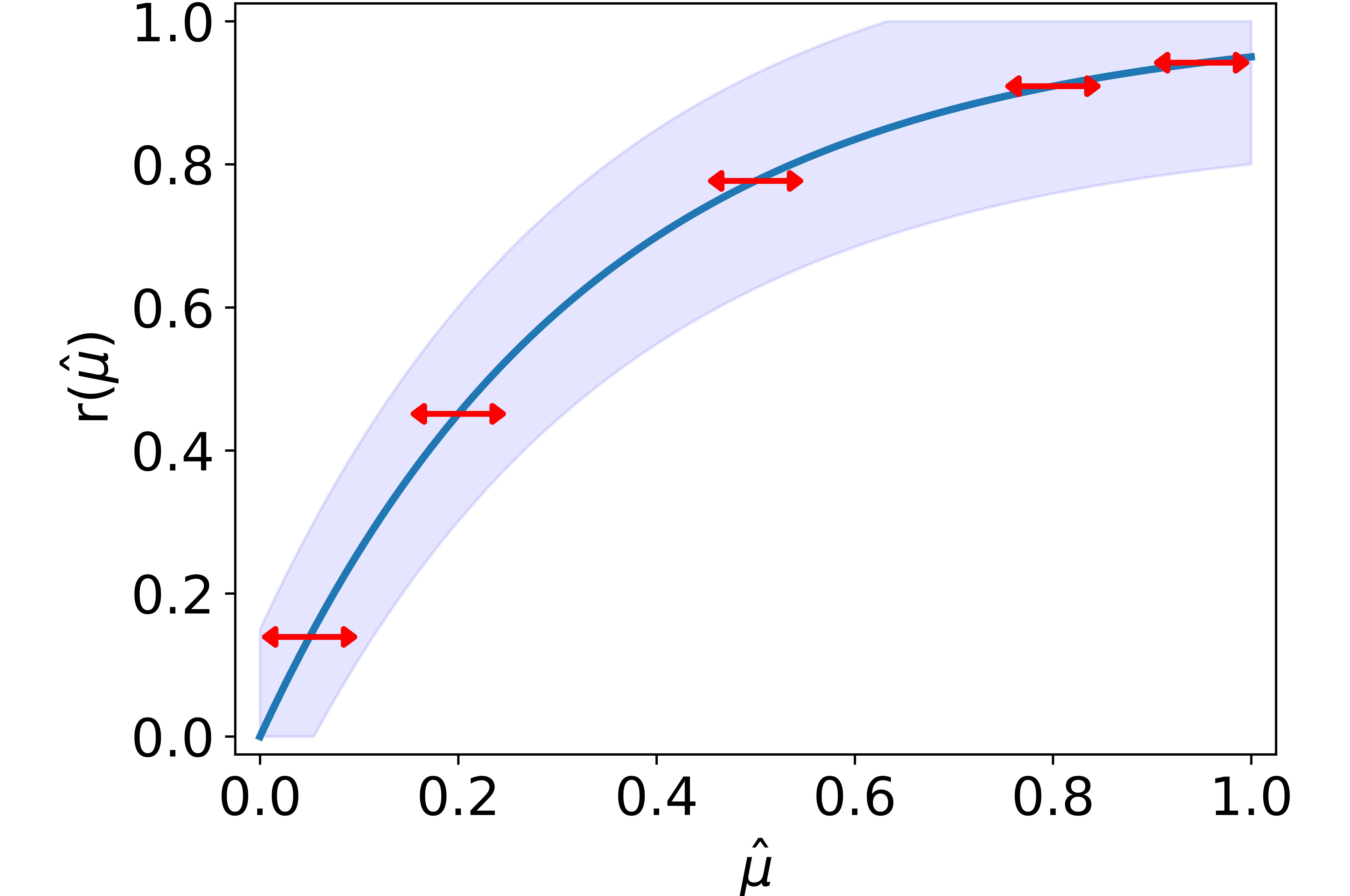
Figure 1: Red arrows: confidence intervals on the function parameter (x-axis confidence), due to either Hoeffding or Bernstein inequalities; the latter is tighter near the edges. Blue zone: the resulting confidence intervals on the reward function in the bold curve (y-axis confidence). In Figures 1,1, these intervals are derived using the global Lipschitz constant of the reward γ∞\gamma_{\infty}, i.e., C​I​(r⁡(𝝁^))≲γ∞​∑iC​I​(μ^i)CI\left(r\left(\hat{\boldsymbol{\mu}}\right)\right)\!\lesssim\!\gamma_{\infty}\sum_{i}CI(\hat{\mu}_{i}). In Figure 1, we present the real confidence interval on the reward, that is much tighter than the bound due to γ∞\gamma_{\infty}. This is since the bound is tight where the gradient is large, which is around the edge of the domain, but loose in other areas, where the gradient is small.

We now present the smoothness measures for smooth index-invariant reward functions that govern our lower bounds. The measures are defined for arm parameters 𝝁∈ℝK{\boldsymbol{\mu}}\!\in\!\mathbb{R}^{K} and a set I⊂[m]I\!\subset\!\left[m\right] as follows:

  1. 1.

    L2 Gini-weighted smoothness

    γg,22​(𝝁,I)\displaystyle\gamma_{g,2}^{2}({\boldsymbol{\mu}};I) ≜∑i=1KIpi𝝁,I​(1−pi𝝁,I)​∇ir​(p𝝁,I)2=∑i∉Iμi​(1−μi)​∇ir​(𝝁)2\displaystyle\triangleq\sum_{i=1}^{K_{I}}p^{{\boldsymbol{\mu}},I}_{i}(1-p^{{\boldsymbol{\mu}},I}_{i})\nabla_{i}r\left(p^{{\boldsymbol{\mu}},I}\right)^{2}=\sum_{i\notin I}\mu_{i}(1-\mu_{i})\nabla_{i}r\left({\boldsymbol{\mu}}\right)^{2} (2)
  2. 2.

    L1 Gini-weighted smoothness

    γg,12​(𝝁,I)\displaystyle\gamma_{g,1}^{2}({\boldsymbol{\mu}};I) ≜(∑i=1KIpi𝝁,I​(1−pi𝝁,I)​∇ir​(p𝝁,I))2=(∑i∉Iμi​(1−μi)​∇ir​(𝝁))2\displaystyle\triangleq\left(\sum_{i=1}^{{K_{I}}}\sqrt{p^{{\boldsymbol{\mu}},I}_{i}(1-p^{{\boldsymbol{\mu}},I}_{i})}\nabla_{i}r\left(p^{{\boldsymbol{\mu}},I}\right)\right)^{2}=\left(\sum_{i\notin I}\sqrt{\mu_{i}(1-\mu_{i})}\nabla_{i}r\left({\boldsymbol{\mu}}\right)\right)^{2} (3)
  3. 3.

    Modified Gini-weighted smoothness

    γ~g2​(𝝁,I)=∑i=1KIpi𝝁,I​(1−pi𝝁,I)​∇ir​(p𝝁,I)2+2​∑i=1KI∑j=i+1KIpi𝝁,I​(1−pj𝝁,I)​∇ir​(p𝝁,I)​∇jr​(p𝝁,I)\displaystyle\tilde{\gamma}_{g}^{2}({\boldsymbol{\mu}};I)=\sum_{i=1}^{K_{I}}p^{{\boldsymbol{\mu}},I}_{i}(1-p^{{\boldsymbol{\mu}},I}_{i})\nabla_{i}r\left(p^{{\boldsymbol{\mu}},I}\right)^{2}+2\sum_{i=1}^{K_{I}}\sum_{j=i+1}^{K_{I}}p^{{\boldsymbol{\mu}},I}_{i}(1-p^{{\boldsymbol{\mu}},I}_{j})\nabla_{i}r\left(p^{{\boldsymbol{\mu}},I}\right)\nabla_{j}r\left(p^{{\boldsymbol{\mu}},I}\right) (4)

Notice that the last equality in Equations (2),(3) is due to the index-invariance assumption. Specifically, the assumption implies that ∇ir​(𝝁)\nabla_{i}r\left({\boldsymbol{\mu}}\right) only depends on μi\mu_{i} and the set of values {μi}i=1m\left\{\mu_{i}\right\}_{i=1}^{m}. For smooth index-invariant reward functions, γg,22​(𝝁,I)\gamma_{g,2}^{2}({\boldsymbol{\mu}};I) is an extension of the Gini-smoothness, as defined in (Merlis and Mannor 2019). In particular, their smoothness parameter is defined as γg=maxI,𝝁⁡γg,2​(𝝁,I)=max𝝁⁡γg,2​(𝝁,∅)\gamma_{g}=\max_{I,{\boldsymbol{\mu}}}\gamma_{g,2}({\boldsymbol{\mu}};I)=\max_{{\boldsymbol{\mu}}}\gamma_{g,2}({\boldsymbol{\mu}};\emptyset). A motivation to this smoothness criterion is presented in Figure 1. Notably, the performance of any algorithm strongly depends on the uncertainty in the reward of actions. However, algorithms only have access to uncertainty in arm parameters, and arm uncertainty must be translated into reward uncertainty. The figure illustrates that doing so using the global Lipschitz constant might lead to loose bounds. Intuitively, if the gradients are small, even wide confidence intervals do not cause high uncertainty in the reward. Similarly, narrow confidence intervals do not lead to high reward uncertainty even where the gradients are large. Thus, Merlis and Mannor 2019 suggested weighting the gradients according to the confidence intervals of the arms. Specifically, their algorithm (BC-UCB) relies on Empirical-Bernstein concentration-bounds (Audibert et al. 2009), that depend on the variance of the arms and are proportional to μi​(1−μi)\sqrt{\mu_{i}(1-\mu_{i})} for Bernoulli arms. Similarly weighting the gradients leads to the Gini-smoothness measures.

In the following sections, we prove lower bounds for the CMAB problem that depend on γ~g2​(𝝁,I)\tilde{\gamma}_{g}^{2}({\boldsymbol{\mu}};I). While complex at first glance, γ~g2​(𝝁,I)\tilde{\gamma}_{g}^{2}({\boldsymbol{\mu}};I) is actually closely related to the other smoothness measures. Notably, observe that the only difference between γ~g2​(𝝁,I)\tilde{\gamma}_{g}^{2}({\boldsymbol{\mu}};I) and γg,12​(𝝁,I)\gamma_{g,1}^{2}({\boldsymbol{\mu}};I) is a small modification to the second (cross) term of (4). In Proposition 3, we indeed prove that γ~g2​(𝝁,I)≥Ω~​(γg,12​(𝝁,I))\tilde{\gamma}_{g}^{2}({\boldsymbol{\mu}};I)\geq\tilde{\Omega}(\gamma_{g,1}^{2}({\boldsymbol{\mu}};I)). When the function is monotone, we later prove that γg,1​(𝝁,I)\gamma_{g,1}({\boldsymbol{\mu}};I) can also be related to γg,2​(𝝁,∅)\gamma_{g,2}({\boldsymbol{\mu}};\emptyset), which leads to tight lower bounds, up to logarithmic factors.

4 Problem-Dependent Lower Bounds

In this section, we prove a problem-dependent lower bound. Specifically, we show that there exist a CMAB instance, such that the asymptotic regret of any consistent strategy on this instance is lower bounded by a logarithmic term that depends on γ~g​(𝝁,I)\tilde{\gamma}_{g}({\boldsymbol{\mu}};I) and the minimal gap Δ=minS∈𝒮,ΔS>0⁡ΔS\Delta=\min_{S\in\mathcal{S},\Delta_{S}>0}\Delta_{S}. Consistent strategy is defined as follows:

Definition 5.

A bandit strategy ψ\psi is called consistent if for any CMAB problem, any S∈𝒮S\in\mathcal{S} such that ΔS>0\Delta_{S}>0 and any 0<α≤10<\alpha\leq 1, it holds that 𝔼⁡[Nψ,S​(T)]=o⁡(Tα)\mathbb{E}\left[N_{\psi,S}(T)\right]=o\left(T^{\alpha}\right).

To prove the lower bounds, we focus on a subset of CMAB problems which we call II-disjoint.

Definition 6.

For a given subset I⊂[m]I\!\subset\!\left[m\right], a CMAB problem is called II-disjoint if all arms i∈Ii\!\in\!I are mutually independent of all arms i∉Ii\!\notin\!I and also S1∩S2=IS_{1}\!\cap\!S_{2}\!=\!I for any S1≠S2∈𝒮S_{1}\!\neq\!S_{2}\!\in\!\mathcal{S}.

Since |S|≤K\lvert S\rvert\leq K, we implicitly assume that |I|≤K\lvert I\rvert\leq K and denote the effective maximal action size by KI=K−|I|{K_{I}}=K-\lvert I\rvert. In II-disjoint CMAB problems, the base arms i∈Ii\in I appear in all actions and are mutually independent of the other arms. The rest of the arms can only appear in one action. This notion of CMAB problems actually extends the action sets from previous work – for the linear reward function, Kveton et al. 2015c divided the arms into mK\frac{m}{K} disjoint groups, which is equivalent to I=∅I\!=\!\emptyset. In contrast, in the CMAB instance on which the PMC lower bounds were derived, only a single arm per item varied between actions (Merlis and Mannor 2019). If there are MM items, this is equivalent to I=[K−M]I\!=\!\left[K-M\right]. We show that choosing the ‘worst-case’ set II naturally results with tighter lower bounds. We start by deriving general problem-dependent lower bound, using Lemma 4:

Lemma 7.

Let rr be a smooth index invariant reward function with |S|=K\left\lvert S\right\rvert=K for all S∈𝒮S\in\mathcal{S}. Also, let ν¯{\underline{\nu}} be the action distribution of an II-disjoint CMAB problem such that there exists an arm i∉Ii\notin I in S∗S^{*} with Pr{Xi(t)=μi}<1\Pr\left\{X^{(t)}_{i}=\mu_{i}\right\}<1 and ∇ir​(S∗,𝛍)≠0\nabla_{i}r\left(S^{*};{\boldsymbol{\mu}}\right)\neq 0. Then, for all consistent strategies ψ\psi and all suboptimal actions SS,

lim infT→∞𝔼ν¯​[Nψ,S​(T)]ln⁡T≥1DKL​(νS,νS∗).\displaystyle\liminf_{T\to\infty}\frac{\mathbb{E}_{\underline{\nu}}\left[N_{\psi,S}(T)\right]}{\ln T}\geq\frac{1}{D_{\mathrm{KL}}(\nu_{S},\nu_{S^{*}})}\kern 4.62497pt.

Specifically, it holds that

lim infT→∞𝔼ν¯​[R​(T)]ln⁡T≥∑S:ΔS>0ΔSDKL​(νS,νS∗).\displaystyle\liminf_{T\to\infty}\frac{\mathbb{E}_{\underline{\nu}}\left[R(T)\right]}{\ln T}\geq\sum_{S:\Delta_{S}>0}\frac{\Delta_{S}}{D_{\mathrm{KL}}(\nu_{S},\nu_{S^{*}})}\kern 4.62497pt.

The proof is in Appendix A, and partially follows Theorem 1 of (Garivier et al. 2018), with some adjustments due to the nonlinearity of the reward function. Although this lemma gives a general lower bound for II-disjoint CMAB problems, it has no clear dependence on any smoothness measure of the reward. To derive lower bounds that directly depend on such measures, we carefully design the arm distributions νS,νS∗\nu_{S},\nu_{S^{*}} and analyze both ΔS\Delta_{S} and DKL​(νS,νS∗)D_{\mathrm{KL}}(\nu_{S},\nu_{S^{*}}) for these distributions. We do so in the following theorem, which results with the desired lower bound:

Theorem 1.

Let rr be a smooth index invariant reward function. For any 𝛍∈[0,1]K{\boldsymbol{\mu}}\in\left[0,1\right]^{K} and any small enough Δ>0\Delta>0, there exists an instance of an II-disjoint bandit problem ν¯{\underline{\nu}} with minimal gap Δ\Delta and 𝔼⁡[νS∗]=𝛍\mathbb{E}\left[\nu_{S^{*}}\right]={\boldsymbol{\mu}}, such that the expected regret of any consistent algorithm is bounded by

lim infT→∞𝔼ν¯​[R​(t)]ln⁡T≥maxI⁡(m−2​K)​γ~g2​(𝝁,I)8​KI​Δ≜D​Br∗​(Δ,𝝁).\displaystyle\liminf_{T\to\infty}\frac{\mathbb{E}_{\underline{\nu}}\left[R(t)\right]}{\ln T}\geq\max_{I}\frac{(m-2K)\tilde{\gamma}_{g}^{2}({\boldsymbol{\mu}};I)}{8{K_{I}}\Delta}\triangleq DB^{*}_{r}(\Delta;{\boldsymbol{\mu}})\kern 4.62497pt.

The result can also be easily extended as follows:

Corollary 8.

Let rr be a smooth index invariant reward function and let 𝛍~=[𝛍1,…,𝛍M]∈[0,1]M​K\tilde{\boldsymbol{\mu}}\!=\!\left[{\boldsymbol{\mu}}_{1},\dots,{\boldsymbol{\mu}}_{M}\right]\!\in\!\left[0,1\right]^{MK}, with 𝛍i∈[0,1]K{\boldsymbol{\mu}}_{i}\in\left[0,1\right]^{K} for all i∈[M]i\in\left[M\right]. Also, define r~​(𝛍~)=∑i=1Mr⁡(𝛍i)\tilde{r}\left(\tilde{\boldsymbol{\mu}}\right)=\sum_{i=1}^{M}r\left({\boldsymbol{\mu}}_{i}\right). Then, for any 𝛍∈[0,1]K{\boldsymbol{\mu}}\in\left[0,1\right]^{K}, there exists a CMAB instance that aims to maximize r~\tilde{r} and has a minimal gap Δ\Delta, such that the optimal action has means 𝛍i=𝛍{\boldsymbol{\mu}}_{i}={\boldsymbol{\mu}} for all i∈[M]i\in\left[M\right] and the expected regret of any consistent algorithm is bounded by

lim infT→∞𝔼ν¯​[R​(t)]ln⁡T≥M2⋅D​Br∗​(Δ,𝝁).\displaystyle\liminf_{T\to\infty}\frac{\mathbb{E}_{\underline{\nu}}\left[R(t)\right]}{\ln T}\geq M^{2}\cdot DB^{*}_{r}(\Delta;{\boldsymbol{\mu}})\kern 4.62497pt.

Notice that for each summand of r~\tilde{r}, KK arms are chosen from a total of mm arms, independently of all other summands. Therefore, the problem can also be formulated as an m~=M​m\tilde{m}=Mm-armed problem, with K~=M​K\tilde{K}=MK selected arms per round. The two formulations are equivalent, and we decided to follow this notation for consistancy with (Merlis and Mannor 2019). The corollary is a direct result of Theorem 1; specifically, by fixing the arm distribution to be identical for all of the summands of r~\tilde{r}, we get r~=M⋅r\tilde{r}=M\cdot r, and since the Gini-smoothness parameters linearly scale with the reward function, the bound naturally follows.

Before proving the theorem, we start with a short discussion on the tightness of the results and the relation to existing upper bounds. One interesting case is when pi𝝁,I=p0p^{{\boldsymbol{\mu}},I}_{i}=p_{0} for all i∈[KI]i\in\left[{K_{I}}\right]. Due to the index invariance, the gradient components are also equal, which results with γ~g2​(𝝁,I)=KI2​p0​(1−p0)​∇ir​(p𝝁,I)2\tilde{\gamma}_{g}^{2}({\boldsymbol{\mu}};I)={K_{I}}^{2}p_{0}(1-p_{0})\nabla_{i}r\left(p^{{\boldsymbol{\mu}},I}\right)^{2}. This choice allows us to easily reproduce the existing lower bounds and leads to the bounds stated in Table 1. Specifically, for the linear reward function, we achieve the bound by choosing I=∅I\!=\!\emptyset and p0=12p_{0}\!=\!\frac{1}{2}; for the PMC problem, we start by writing r~=∑i=1Mr⁡(S,𝝁i)\tilde{r}=\sum_{i=1}^{M}r\left(S;{\boldsymbol{\mu}}_{i}\right) for r⁡(S,𝝁)=1−∏j∈Sμjr\left(S;{\boldsymbol{\mu}}\right)=1-\prod_{j\in S}\mu_{j}. Then, we apply Theorem 1 on rr and choose the subset II such that it contains all arms except for a single (first) element from each vector 𝝁i=(12,0,…,0){\boldsymbol{\mu}}_{i}=\left(\frac{1}{2},0,\dots,0\right), i.e., KI=1{K_{I}}=1 and p0=12p_{0}=\frac{1}{2}. The lower bound is then a direct result of Corollary 8. We remark that although choosing KI=K{K_{I}}=K is seemingly optimal, this is not always the case. A notable example for this issue is the reward function r(S;𝝁)=1−e−∑i∈Sμi2r\left(S;{\boldsymbol{\mu}}\right)=1-e^{-\sum_{i\in S}\mu_{i}^{2}}. For this instance, optimizing over p0p_{0} leads to a bound of γ~g2​(𝝁,I)/KI=Ω⁡(1/KI)\tilde{\gamma}_{g}^{2}({\boldsymbol{\mu}};I)/{K_{I}}=\Omega\left(1/\sqrt{{K_{I}}}\right), and the optimal choice is KI=𝒪⁡(1){K_{I}}=\mathcal{O}(1). In this example it also holds that γg=𝒪⁡(1)\gamma_{g}=\mathcal{O}(1), and, therefore, this bound is tight.

We note that this bound only requires the smooth index invariance assumption and holds for non-monotone reward functions. When the reward is also monotone, observe that γ~g2​(𝝁,I)≥γg,22​(𝝁,I)\tilde{\gamma}_{g}^{2}({\boldsymbol{\mu}};I)\geq\gamma_{g,2}^{2}({\boldsymbol{\mu}};I). Choosing I=∅I=\emptyset and maximizing over 𝝁{\boldsymbol{\mu}} leads to a lower bound of Ω⁡(m​γg2​ln⁡TΔ​K)\Omega\left(\frac{m\gamma_{g}^{2}\ln T}{\Delta K}\right), which differs from the upper bound of (Merlis and Mannor 2019) by a factor of KK. We later prove that when the reward is monotone, a stronger lower bound can be derived, such that it matches the upper bound up to logarithmic factors.

Next, we present the proof of Theorem 1 which is composed of three parts. We first present a carefully designed parametric arm distributions, that allow controlling the suboptimality gap while retaining low KL-divergence. We then bound both the gap and the KL-divergence in terms of the parameters of the distributions and apply Lemma 7 using these bounds. We conclude the proof by optimizing the resulting lower bound over the distribution parameters.

Proof.

Step 1: Fixing a parametric family of CMAB instances.

Denote by I∗I^{*}, the maximizer of II in D​Br∗​(Δ,𝝁)DB^{*}_{r}(\Delta;{\boldsymbol{\mu}}), and for brevity, let p=p𝝁,I∗p=p^{{\boldsymbol{\mu}},I^{*}} and KI=KI∗=K−|I∗|{K_{I}}={K_{I}}^{*}=K-\left\lvert I^{*}\right\rvert. Note that this also implies that 0≤p1≤⋯≤pKI≤10\leq p_{1}\leq\dots\leq p_{K_{I}}\leq 1. In addition, due to the form of the lower bound, we can deduce that p1>0p_{1}>0 and pKI<1p_{K_{I}}<1, since otherwise, we can move arms with means 0 and 1 into I∗I^{*} and strictly increase D​Br∗​(Δ,𝝁)DB^{*}_{r}(\Delta;{\boldsymbol{\mu}}). For now, we also assume that no two arms have the same mean, i.e., 0<p1<⋯<pKI<10<p_{1}<\dots<p_{K_{I}}<1, and will return to this assumption later in the proof. Without loss of generality, we also assume that KI>0{K_{I}}>0 and there exists i∈[KI]i\in\left[{K_{I}}\right] such that ∇ir​(p)≠0\nabla_{i}r\left(p\right)\!\neq\!0 since otherwise, D​Br∗​(Δ,𝝁)=0DB^{*}_{r}(\Delta;{\boldsymbol{\mu}})\!=\!0 and trivially holds. Similarly, we assume that m>2​Km\!>\!2K.

Table 2: The probability distributions ν\nu and ν∗\nu^{*} of arms outside I∗I^{*}, with parameters <p1<p2<…<pKI<10\!<\!p_{1}\!<\!p_{2}\!<\!\dots\!<\!p_{K_{I}}\!<\!1 and ϵ∈ℝKI\epsilon\in\mathbb{R}^{K_{I}}. Arms in I∗I^{*} have mean 𝝁I∗{\boldsymbol{\mu}}_{I^{*}} and are independent of the rest of the arms.
Observation vector Probability of Probability of
X(t)=(X1(t),⋯,XKI(t))X^{(t)}\!\!=\!\left(X^{(t)}_{1},\cdots,X^{(t)}_{{K_{I}}}\right) X(t)X^{(t)} in ν∗\nu^{*} X(t)X^{(t)} in ν\nu
(1,1,⋯,1,1)(1,1,\cdots,1,1) p1p_{1} p1−ϵ1p_{1}-\epsilon_{1}
(0,1,⋯,1,1)(0,1,\cdots,1,1) p2−p1p_{2}-p_{1} p2−p1−ϵ2p_{2}-p_{1}-\epsilon_{2}
⋯\cdots ⋯\cdots ⋯\cdots
(0,0,⋯,0,1)(0,0,\cdots,0,1) pKI−pKI−1p_{K_{I}}-p_{{K_{I}}-1} pKI−pKI−1−ϵKIp_{K_{I}}-p_{{K_{I}}-1}-\epsilon_{K_{I}}
(0,0,⋯,0,0)(0,0,\cdots,0,0) 1−pKI1-p_{K_{I}} 1−pKI+∑i=jKIϵj1-p_{K_{I}}+\sum_{i=j}^{K_{I}}\epsilon_{j}

We fix the CMAB problem to be I∗I^{*}-disjoint, and choose the action set 𝒮\mathcal{S} to be the maximal action set with action sizes KK, i.e., |𝒮|=⌊m−|I∗|K−|I∗|⌋≥m−KKI\lvert\mathcal{S}\rvert=\left\lfloor\frac{m-\lvert I^{*}\rvert}{K-\lvert I^{*}\rvert}\right\rfloor\geq\frac{m-K}{{K_{I}}}. Denote the arm distribution in this problem by ν¯{\underline{\nu}}, and fix the distribution of the common arms i∈I∗i\in I^{*} to any distribution with expectation 𝔼⁡[νI∗]=𝝁I∗\mathbb{E}\left[\nu_{I^{*}}\right]={\boldsymbol{\mu}}_{I^{*}}, as long as they are mutually independent of the rest of the arms. For a single action, we set the distribution to be ν∗\nu^{*} with mean 𝝁ν∗≜𝝁{\boldsymbol{\mu}}^{\nu^{*}}\triangleq{\boldsymbol{\mu}}, and for the rest of the actions, we fix it to distribution ν\nu with mean 𝝁ν{\boldsymbol{\mu}}^{\nu}. Both distributions are stated in Table 2. The distribution ν\nu depends on ϵ∈ℝKI\epsilon\in\mathbb{R}^{K_{I}}, that will be determined later such that ν\nu is strictly suboptimal, and we denote its suboptimality gap by Δϵ=r⁡(𝝁ν∗)−r⁡(𝝁ν)\Delta_{\epsilon}=r\left({\boldsymbol{\mu}}^{\nu^{*}}\right)-r\left({\boldsymbol{\mu}}^{\nu}\right). We remark that for <p1<…<pKI<10\!<\!p_{1}\!<\!\dots\!<\!p_{K_{I}}\!<\!1, there exists bϵ,0b_{\epsilon,0} such that ν\nu is a valid probability distribution for all ‖ϵ‖∞≤bϵ,0\left\lVert\epsilon\right\rVert_{\infty}\leq b_{\epsilon,0}. We enforce this condition later in the proof.

Note that for all i∉I∗i\notin I^{*}, the arms are Bernoulli random variables with mean μi∉{0,1}\mu_{i}\notin\left\{0,1\right\}, and therefore Pr{Xi(t)=pi}=0\Pr\left\{X^{(t)}_{i}=p_{i}\right\}=0. Also, since the gradient is not zero for some i∉I∗i\notin I^{*}, the conditions of Lemma 7 hold, and we can bound the regret by

lim infT→∞𝔼ν¯​[R​(T)]ln⁡T\displaystyle\liminf_{T\to\infty}\frac{\mathbb{E}_{\underline{\nu}}\left[R(T)\right]}{\ln T} ≥∑i=1|𝒮|−1ΔϵDKL​(ν,ν∗)≥m−2​KKI​ΔϵDKL​(ν,ν∗).\displaystyle\geq\sum_{i=1}^{\lvert\mathcal{S}\rvert-1}\frac{\Delta_{\epsilon}}{D_{\mathrm{KL}}(\nu,\nu^{*})}\geq\frac{m-2K}{{K_{I}}}\frac{\Delta_{\epsilon}}{D_{\mathrm{KL}}(\nu,\nu^{*})}\kern 4.62497pt. (5)

Step 2: Deriving lower bounds that depend on the distribution parameters ϵ\epsilon.

Next, we bound both DKL​(ν,ν∗)D_{\mathrm{KL}}(\nu,\nu^{*}) and Δϵ\Delta_{\epsilon} in terms of ϵ\epsilon.

Lemma 9.

Let p≜p𝛍,I∈ℝKp\triangleq p^{{\boldsymbol{\mu}},I}\in\mathbb{R}^{K} such that 0<p1<⋯<pKI<10<p_{1}<\dots<p_{K_{I}}<1 and define p0=0p_{0}=0. Also, let ν,ν∗\nu,\nu^{*} be the distributions stated in Table 2. Then, there exists a constant bϵ,1>0b_{\epsilon,1}>0 such that for any ϵ∈ℝKI\epsilon\in\mathbb{R}^{K_{I}} with ‖ϵ‖∞≤bϵ,1\left\lVert\epsilon\right\rVert_{\infty}\leq b_{\epsilon,1}, it holds that

DKL​(ν,ν∗)≤2​ϵT​BK​L​(p)​ϵ,\displaystyle D_{\mathrm{KL}}(\nu,\nu^{*})\leq 2\epsilon^{T}B_{KL}(p)\epsilon\kern 4.62497pt, (6)

where BK​L​(p)=D⁡(p)+11−pKI​𝟏𝟏TB_{KL}(p)=D(p)+\frac{1}{1-p_{K_{I}}}\mathbf{1}\mathbf{1}^{T}, D⁡(p)∈ℝKI×KID(p)\in\mathbb{R}^{{K_{I}}\times{K_{I}}} is a diagonal matrix whose elements are Di​i​(p)=1pi−pi−1D_{ii}(p)=\frac{1}{p_{i}-p_{i-1}} and 𝟏∈ℝKI\mathbf{1}\in\mathbb{R}^{K_{I}} is a vector of ones.

Lemma 10.

Let rr be a smooth index invariant reward function and let p∈ℝKp\in\mathbb{R}^{K} such that 0<p1≤⋯≤pKI<10<p_{1}\leq\dots\leq p_{K_{I}}<1 and there exists i∈[KI]i\in\left[{K_{I}}\right] with ∇ir​(p)≠0\nabla_{i}r\left(p\right)\neq 0. Also, define cj=∑i=jKI∇ir​(p)c_{j}=\sum_{i=j}^{K_{I}}\nabla_{i}r\left(p\right) for all j∈[KI]j\in\left[{K_{I}}\right] and let u∈ℝKIu\in\mathbb{R}^{K_{I}} be a vector such that cT​u>0c^{T}u>0. Then, if ϵ=ϵ0​u\epsilon=\epsilon_{0}u, there exists a constant bϵ,2>0b_{\epsilon,2}>0 such that for all 0<ϵ0≤bϵ,20<\epsilon_{0}\leq b_{\epsilon,2},

Δϵ≥12​cT​ϵ>0.\displaystyle\Delta_{\epsilon}\geq\frac{1}{2}c^{T}\epsilon>0\kern 4.62497pt. (7)

The proofs are presented in Appendix B. Specifically, note that Di​i​(p)>0D_{ii}(p)>0, and thus BK​L​(p)B_{KL}(p) is positive definite, and the KL bound equals zero only for ϵ=0\epsilon=0. Also, since there exists i∈[KI]i\in\left[{K_{I}}\right] such that ∇ir​(p)≠0\nabla_{i}r\left(p\right)\neq 0, it holds that c≠0c\neq 0. When both lemmas hold, substitution into (5) yields

lim infT→∞𝔼ν¯​[R​(T)]ln⁡T\displaystyle\liminf_{T\to\infty}\frac{\mathbb{E}_{\underline{\nu}}\left[R(T)\right]}{\ln T} ≥m−2​KKI​ΔϵDKL​(ν¯,ν¯∗)=m−2​KKI​Δϵ​Δϵ2DKL​(ν¯,ν¯∗)≥m−2​K8​KI​Δϵ​(cT​ϵ)2ϵT​BK​L​(p)​ϵ.\displaystyle\geq\frac{m-2K}{{K_{I}}}\frac{\Delta_{\epsilon}}{D_{\mathrm{KL}}({\underline{\nu}},{\underline{\nu}}^{*})}=\frac{m-2K}{{K_{I}}\Delta_{\epsilon}}\frac{\Delta_{\epsilon}^{2}}{D_{\mathrm{KL}}({\underline{\nu}},{\underline{\nu}}^{*})}\geq\frac{m-2K}{8{K_{I}}\Delta_{\epsilon}}\frac{\left(c^{T}\epsilon\right)^{2}}{\epsilon^{T}B_{KL}(p)\epsilon}\kern 4.62497pt. (8)

Step 3: Finding the worst-case CMAB instance.

We now focus on the function fI​(ϵ,p)=ϵT​c​cT​ϵϵT​BK​L​(p)​ϵf_{I}(\epsilon;p)=\frac{\epsilon^{T}cc^{T}\epsilon}{\epsilon^{T}B_{KL}(p)\epsilon}, which is defined for any ϵ≠0\epsilon\neq 0, as BK​L​(p)B_{KL}(p) is positive definite. BK​L​(p)B_{KL}(p) is also invertible, and we can therefore apply the invertible transformation ϵ=BK​L−1/2(p)x\epsilon=B_{KL}^{-1/2}(p)x, which results with the following function:

f~I​(x,p)\displaystyle\tilde{f}_{I}(x;p) =xTBK​L−1/2(p)ccTBK​L−1/2(p)x∥x∥22=(cTBK​L−1/2(p)x)2∥x∥22≤(∗)∥BK​L−1/2(p)c∥22∥x∥22∥x∥22=cT​BK​L−1​(p)​c,\displaystyle=\frac{x^{T}B_{KL}^{-1/2}(p)cc^{T}B_{KL}^{-1/2}(p)x}{\lVert x\rVert_{2}^{2}}=\frac{\left(c^{T}B_{KL}^{-1/2}(p)x\right)^{2}}{\lVert x\rVert_{2}^{2}}\stackrel{{\scriptstyle(*)}}{{\leq}}\frac{\lVert B_{KL}^{-1/2}(p)c\rVert_{2}^{2}\lVert x\rVert_{2}^{2}}{\lVert x\rVert_{2}^{2}}=c^{T}B_{KL}^{-1}(p)c\kern 4.62497pt,

where (∗)(*) is due to Cauchy-Schwarz Inequality, and equality holds for any ϵ0≠0\epsilon_{0}\neq 0 and x=ϵ0BK​L−1/2(p)cx=\epsilon_{0}B^{-1/2}_{KL}(p)c. Therefore, the maximal value of fI​(ϵ,p)f_{I}(\epsilon;p) is fI​(ϵ∗,p)=cT​BK​L−1​(p)​cf_{I}(\epsilon^{*};p)=c^{T}B^{-1}_{KL}(p)c and can be attained with ϵ∗=ϵ0​BK​L−1​(p)​c\epsilon^{*}=\epsilon_{0}B^{-1}_{KL}(p)c, for any ϵ0≠0\epsilon_{0}\neq 0.

Motivated by the maximization property of ϵ∗\epsilon^{*}, we now fix ϵ←ϵ∗=ϵ0​BK​L−1​(p)​c\epsilon\leftarrow\epsilon^{*}=\epsilon_{0}B_{KL}^{-1}(p)c, for 0<ϵ0≤bϵ,20<\epsilon_{0}\leq b_{\epsilon,2} such that ‖ϵ∗‖∞≤min⁡{bϵ,0,bϵ,1}\left\lVert\epsilon^{*}\right\rVert_{\infty}\leq\min\left\{b_{\epsilon,0},b_{\epsilon,1}\right\}. For this choice, ϵ∗≠0\epsilon^{*}\neq 0, since BK​L​(p)B_{KL}(p) is invertible and c≠0c\neq 0, and cT​BK​L−1​(p)​c>0c^{T}B_{KL}^{-1}(p)c>0 as required for Lemma 10. We explicitly calculate the lower bound in the following lemma (see proof in Appendix B):

Lemma 11.

Under the notations of Lemmas 9 and 10, for any <p1<…<pKI<10\!<\!p_{1}\!<\!\dots\!<\!p_{K_{I}}\!<\!1 and c≠0c\neq 0, if ϵ∗=ϵ0​BK​L−1​(p)​c\epsilon^{*}=\epsilon_{0}B_{KL}^{-1}(p)c, then

ϵi∗=ϵ0​(pi−pi−1)​(ci−∑j=1KI(pj−pi−j)​cj).\displaystyle\epsilon^{*}_{i}=\epsilon_{0}\left(p_{i}-p_{i-1}\right)\left(c_{i}-\sum_{j=1}^{K_{I}}\left(p_{j}-p_{i-j}\right)c_{j}\right)\kern 4.62497pt.

Also, if fI​(ϵ,p)=ϵT​c​cT​ϵϵT​BK​L​(p)​ϵf_{I}(\epsilon;p)\!=\!\frac{\epsilon^{T}cc^{T}\epsilon}{\epsilon^{T}B_{KL}(p)\epsilon}, then fI​(ϵ∗,p)=γ~g2​(𝛍,I)f_{I}(\epsilon^{*};p)\!=\!\tilde{\gamma}_{g}^{2}({\boldsymbol{\mu}};I).

An important conclusion is that under the assumptions of the lemma, γ~g2​(𝝁,I)>0\tilde{\gamma}_{g}^{2}({\boldsymbol{\mu}};I)>0, since fI​(ϵ∗,p)=cT​BK​L−1​(p)​c>0f_{I}(\epsilon^{*};p)=c^{T}B_{KL}^{-1}(p)c>0. A more general result naturally arises from the proof of Lemma 11: for any for any 𝝁∈[0,1]K{\boldsymbol{\mu}}\in\left[0,1\right]^{K} and any I⊂[K]I\subset\left[K\right], it holds that γ~g2​(𝝁,I)≥0\tilde{\gamma}_{g}^{2}({\boldsymbol{\mu}};I)\geq 0, as expected from a smoothness parameter. We refer the readers to the proof of the lemma for additional details. Substituting back into (8) and recalling that I∗I^{*} was chosen as the maximizer in D​Br∗​(Δ,𝝁)DB^{*}_{r}(\Delta;{\boldsymbol{\mu}}) we get

lim infT→∞𝔼ν¯​[R​(T)]ln⁡T\displaystyle\liminf_{T\to\infty}\frac{\mathbb{E}_{\underline{\nu}}\left[R(T)\right]}{\ln T} ≥(m−2​K)​γ~g2​(𝝁,I∗)​(p)8​KI∗​Δϵ=D​Br∗​(Δϵ,𝝁).\displaystyle\geq\frac{(m-2K)\tilde{\gamma}_{g}^{2}({\boldsymbol{\mu}};I^{*})(p)}{8{K_{I}}^{*}\Delta_{\epsilon}}=DB^{*}_{r}(\Delta_{\epsilon};{\boldsymbol{\mu}}).

We finally return to our assumption that p1<⋯<pKIp_{1}<\dots<p_{K_{I}}. If there are equal values in pp, i.e., pi=pi=⋯=pi+n−1p_{i}=p_{i}=\dots=p_{i+n-1}, we modify both distributions in Table 2 such that the observations of these arms are identical, namely Xi(t)=Xi+1(t)=⋯=Xi+n−1(t)X^{(t)}_{i}=X^{(t)}_{i+1}=\dots=X^{(t)}_{i+n-1}. Then, we set ϵi+1∗=⋯=ϵi+n−1∗=0\epsilon^{*}_{i+1}=\dots=\epsilon^{*}_{i+n-1}=0. Notice that this modification does not change the KL divergence, nor the analysis of the gap, and therefore retains the same results. Similarly, Lemma 11 still holds by defining the function fIf_{I} over the sub-vector of ϵ\epsilon with coordinates such that pi<pi+1p_{i}<p_{i+1}. Alternatively, note that the existing analysis naturally sets ϵi=0\epsilon_{i}=0 if pi=pi−1p_{i}=p_{i-1} (Lemma 11), so it is not surprising that this modification does not change the results. We avoided writing the full analysis since it requires indexing the sub-vector of pp with strictly increasing values, which would make the notations much more involved.

To conclude the proof, we remark that if Δ0>0\Delta_{0}>0 is the gap for some ϵ0>0\epsilon_{0}>0 such that Lemmas 9 and 10 hold, by tuning ϵ0\epsilon_{0} we can achieve any gap Δ≤Δ0\Delta\leq\Delta_{0}, and thus the previous result holds for any small enough gap Δ\Delta. ∎

5 Problem-Independent Lower Bounds

In this section, we prove a problem-independent regret lower bound. Specifically, we prove that for any fixed strategy and any large enough horizon TT, there exists a CMAB instance such that the regret is lower bounded by a gap-independent T\sqrt{T} term. We remark that in contrast to problem-dependent bounds, in which the instance is fixed for all strategies and time horizons, the instance for problem-independent bounds is designed as the ‘worst-case’ problem for a specific strategy and time horizon. Similarly to the previous section, we start by proving a general lower bound for II-disjoint CMAB problems and then apply it with a specific distribution to derive the desired bound.

Lemma 12.

Let rr be a smooth index invariant reward function, and let I⊂[m]I\subset\left[m\right] such that |I|≤K\left\lvert I\right\rvert\leq K and m>Km>K. Also, let 𝛍,𝛍∗∈ℝK{\boldsymbol{\mu}},{\boldsymbol{\mu}}^{*}\in\mathbb{R}^{K} such that 𝛍I=𝛍I∗{\boldsymbol{\mu}}_{I}={\boldsymbol{\mu}}^{*}_{I} and Δ=r⁡(𝛍∗)−r⁡(𝛍)>0\Delta=r\left({\boldsymbol{\mu}}^{*}\right)-r\left({\boldsymbol{\mu}}\right)>0. Finally, let ν,ν∗\nu,\nu^{*} be two distributions with expectations 𝛍,𝛍∗∈ℝK{\boldsymbol{\mu}},{\boldsymbol{\mu}}^{*}\in\mathbb{R}^{K}, such that arms in II are mutually independent of arms outside II and both distributions are identical for arms in II. Then, for any horizon TT and any strategy ψ\psi, there exists an II-disjoint CMAB problem with arm distribution ν¯′{\underline{\nu}}^{\prime} such that νS∗=𝛍∗\nu_{S^{*}}={\boldsymbol{\mu}}^{*} and its regret under strategy ψ\psi is bounded by

𝔼ν¯′​[R⁡(T)]≥T​Δ​(1−KIm−K−12​T​KIm−K​DKL​(ν,ν∗)).\displaystyle\mathbb{E}_{{\underline{\nu}}^{\prime}}\left[R(T)\right]\!\geq\!T\Delta\left(\!1-\frac{{K_{I}}}{m-K}-\sqrt{\frac{1}{2}\frac{T{K_{I}}}{m-K}D_{\mathrm{KL}}(\nu,\nu^{*})}\right)\!.

The proof is a variant of Theorem 6 of Garivier et al. 2018 and can be found in Appendix A. With this lemma at hand, and similarly to the problem-dependent bound of Theorem 1, we can also derive a problem-independent lower bound:

Theorem 2.

Let rr be a smooth index invariant reward function and assume that m≥3​Km\geq 3K. Then, for any 𝛍∈[0,1]K{\boldsymbol{\mu}}\!\in\!\left[0,1\right]^{K}, any T≥T0T\!\geq\!T_{0} and for any strategy ψ\psi, there exists an II-disjoint CMAB problem ν¯′{\underline{\nu}}^{\prime} with 𝔼⁡[νS∗′]=𝛍\mathbb{E}\left[\nu^{\prime}_{S^{*}}\right]={\boldsymbol{\mu}} such that its regret under strategy ψ\psi is bounded by

𝔼ν¯′​[R⁡(T)]≥maxI⁡γ~g​(𝝁,I)32​T⁡(m−K)KI≜I​Br∗​(𝝁).\displaystyle\mathbb{E}_{{\underline{\nu}}^{\prime}}\left[R(T)\right]\geq\max_{I}\frac{\tilde{\gamma}_{g}({\boldsymbol{\mu}};I)}{32}\sqrt{\frac{T(m-K)}{{K_{I}}}}\triangleq IB^{*}_{r}({\boldsymbol{\mu}})\kern 4.62497pt.

Similarly to Corollary 8, the result can also be easily extended to sums as follows:

Corollary 13.

Under the notations of Corollary 8, if m≥3​Km\geq 3K, then for any 𝛍∈[0,1]K{\boldsymbol{\mu}}\!\in\!\left[0,1\right]^{K}, any T≥T0T\!\geq\!T_{0} and for any strategy ψ\psi, there exists CMAB problem ν¯′{\underline{\nu}}^{\prime} such that the optimal action has means 𝛍i=𝛍{\boldsymbol{\mu}}_{i}={\boldsymbol{\mu}} for all i∈[M]i\in\left[M\right] whose regret under strategy ψ\psi is bounded by

𝔼ν¯′​[R⁡(T)]≥M⋅I​Br∗​(𝝁).\displaystyle\mathbb{E}_{{\underline{\nu}}^{\prime}}\left[R(T)\right]\geq M\cdot IB^{*}_{r}({\boldsymbol{\mu}})\kern 4.62497pt.

We defer the proof of the theorem to Appendix C, and the corollary can be proven similarly to Corollary 8. The same discussion from the previous section about the tightness of the bound still holds. We start by noting that I​Br∗​(𝝁)IB^{*}_{r}({\boldsymbol{\mu}}) reproduces the existing lower bounds both for the linear reward function (Kveton et al. 2015c) and the probabilistic maximum coverage problem (Merlis and Mannor 2019). Also, for monotone functions, we can bound γ~g2​(𝝁,∅)≥γg2\tilde{\gamma}_{g}^{2}({\boldsymbol{\mu}};\emptyset)\geq\gamma_{g}^{2} and match the problem-independent upper bound of (Merlis and Mannor 2019) up to a K\sqrt{K} factor. This factor will be improved to a logarithmic factor in the following section.

6 Relations Between Smoothness Measures

To this point, we derived lower bounds that depend on the modified Gini-smoothness γ~g​(𝝁,I)\tilde{\gamma}_{g}({\boldsymbol{\mu}};I). In this section, we show that at a cost of logarithmic factors, we can relate these bounds to the L1 Gini-smoothness. Moreover, for monotone reward functions, we also prove lower bounds that depend on the L2 Gini-smoothness, and thus match the upper bounds of (Merlis and Mannor 2019) up to log-factors. We formally state the results in the following propositions:

Proposition 3.

Let rr be a smooth index invariant reward function and denote p=p𝛍,Ip=p^{{\boldsymbol{\mu}},I} for some 𝛍∈ℝK{\boldsymbol{\mu}}\in\mathbb{R}^{K} and I⊂[K]I\subset\left[K\right]. Then,

γ~g2​(𝝁,I)≥γg,12​(𝝁,I)3+ln⁡1p1+ln⁡11−pKI,\displaystyle\tilde{\gamma}_{g}^{2}({\boldsymbol{\mu}};I)\geq\frac{\gamma_{g,1}^{2}({\boldsymbol{\mu}};I)}{3+\ln\frac{1}{p_{1}}+\ln\frac{1}{1-p_{K_{I}}}}\kern 4.62497pt, (9)

where the r.h.s. is defined as zero if p1=0p_{1}=0 or pKI=1p_{K_{I}}=1.

Proposition 4.

Let rr be a monotone smooth index invariant reward function. Then, for any 𝛍∈ℝK{\boldsymbol{\mu}}\in\mathbb{R}^{K}, it holds that

maxI\displaystyle\max_{I} γg,12​(𝝁,I)KI≥γg,22​(𝝁,∅)1+ln⁡K.\displaystyle\frac{\gamma_{g,1}^{2}({\boldsymbol{\mu}};I)}{{K_{I}}}\geq\frac{\gamma_{g,2}^{2}({\boldsymbol{\mu}};\emptyset)}{1+\ln K}\kern 4.62497pt. (10)

Furthermore, if μmin=mini:μi>0μi\mu_{\min}\!=\!\min_{i:\mu_{i}>0}\mu_{i} and μmax=maxi:μi<1μi\mu_{\max}\!=\!\max_{i:\mu_{i}<1}\mu_{i}, then

maxI\displaystyle\max_{I} γ~g2​(𝝁,I)KI≥γg,22​(𝝁,∅)(1+ln⁡K)​(3+ln⁡1μmin+ln⁡11−μmax).\displaystyle\frac{\tilde{\gamma}_{g}^{2}({\boldsymbol{\mu}};I)}{{K_{I}}}\!\geq\!\frac{\gamma_{g,2}^{2}({\boldsymbol{\mu}};\emptyset)}{\left(1+\ln K\right)\left(3+\ln\frac{1}{\mu_{\min}}+\ln\frac{1}{1-\mu_{\max}}\right)}.

We emphasize that Proposition 3 does not require the monotonicity assumption. However, when the components of the gradient can be either positive or negative, the bound might equal zero even when the gradient is large. When the function is monotone, Proposition 4 greatly improves the naïve choice of I=∅I=\emptyset in the bounds of Theorems 1 and 2, by a factor of KK, with only a logarithmic cost. Specifically, by maximizing over 𝝁{\boldsymbol{\mu}} and applying Proposition 4, we get a problem-dependent lower bound of Ω~​(m​γg2​ln⁡T/Δ)\tilde{\Omega}\left(m\gamma_{g}^{2}\ln T/\Delta\right) and a problem-independent bound of Ω~​(γg​m​T)\tilde{\Omega}\left(\gamma_{g}\sqrt{mT}\right), both match the upper bounds of (Merlis and Mannor 2019) up to log-factors. Thus, for monotone smooth functions, we conclude that the L2 Gini-smoothness parameter characterizes both the upper and lower bounds.

Of the log-factors in the propositions, the more interesting one is that of (ln⁡1μmin+ln⁡11−μmax)\left(\ln\frac{1}{\mu_{\min}}+\ln\frac{1}{1-\mu_{\max}}\right). In cases where the mean values 𝝁{\boldsymbol{\mu}} are exponentially close to zero or one, this factor can be of order 1/K1/K. We suspect that this is due to a proof artefact, but leave the investigation of this factor to future work. Nonetheless, for any practical example, this term is at most of order ln⁡K\ln K, which leaves the bound tight up to log-factors in the problem size. Another question that arises is whether this factor is the result of a loose analysis in Proposition 3, and a tighter analysis might yield a better factor (e.g., ln⁡K\ln K). Sadly, the answer is negative. In Appendix E.1, we build an example where μi\mu_{i} are exponentially small and Inequality (9) does not hold without a factor of order 1/K1/K. Therefore, to remove this factor, D​Br∗​(Δ,𝝁)DB^{*}_{r}(\Delta;{\boldsymbol{\mu}}) and I​Br∗​(𝝁)IB^{*}_{r}({\boldsymbol{\mu}}) also need to be improved.

Due to space limitations, we defer the full proofs to Appendix D and only provide a proof sketch for Proposition 4:

Proof Sketch Notice that γg,1​(𝝁,I)\gamma_{g,1}({\boldsymbol{\mu}};\!I) and γg,2​(𝝁,I)\gamma_{g,2}({\boldsymbol{\mu}};\!I) are closely related to the L1 and L2 norms of a vector whose components are μi​(i−μi)​∇i​r​(𝝁)\sqrt{\mu_{i}(i-\mu_{i})}\nabla_{i}r\left({\boldsymbol{\mu}}\right). Specifically, both are norms of a vector with a subset of these components. We utilize this connection and derive, to the best of our knowledge, a new relation between the norms:

Lemma 14.

Let AA be a nonempty subset of indices A⊂[n]A\subset\left[n\right]. For any vector x∈ℝnx\in\mathbb{R}^{n}, it holds that

maxA≠∅⁡1|A|​‖xA‖12≥11+ln⁡n​∥x∥22.\displaystyle\max_{A\neq\emptyset}\frac{1}{\left\lvert A\right\rvert}\left\lVert x_{A}\right\rVert_{1}^{2}\geq\frac{1}{1+\ln n}\lVert x\rVert_{2}^{2}\kern 4.62497pt.

This lemma gives a much stronger relation than the standard L1-L2 inequality and is of independent interest. Specifically, the relation between the norms is logarithmic in the vector dimension, instead of the standard relation ‖x‖1≥‖x‖2\left\lVert x\right\rVert_{1}\geq\left\lVert x\right\rVert_{2}, that would have resulted in a linear term. This is due to the ability to choose the best subset of the vector on the left-hand side. We remark that this inequality is tight, as demonstrated in Appendix E.2. By applying Lemma 14, we get maxI⁡γg,12​(𝝁,I)KI≥γg,22​(𝝁,∅)1+ln⁡K\max_{I}\frac{\gamma_{g,1}^{2}({\boldsymbol{\mu}};I)}{{K_{I}}}\geq\frac{\gamma_{g,2}^{2}({\boldsymbol{\mu}},\emptyset)}{1+\ln K}, and substituting in Proposition 3 concludes the proof. \jmlrQED

7 Summary and Future Work

In this work, we presented the first lower bounds for the CMAB problem that hold for general reward functions, under very mild assumptions. Specifically, we proved both problem-dependent and problem-independent lower bounds, which depend on the modified Gini-smoothness γ~g​(𝝁,I)\tilde{\gamma}_{g}({\boldsymbol{\mu}};I) and reproduce the existing bounds for specific instances. When the reward function is also monotone, we showed that the upper bounds of (Merlis and Mannor 2019), which depend on the L2 Gini smoothness of the reward function, are tight up to logarithmic factors. There are a few directions for extending our results that we leave for future work:

Gini-smoothness and non-monotone reward functions: One question that naturally arises is whether the L2 Gini-smoothness γg\gamma_{g} also characterizes the lower bound for non-monotone reward function. If such dependence truly holds, a possible way to derive these bounds is by improving γ~g​(𝝁,I)\tilde{\gamma}_{g}({\boldsymbol{\mu}};I) such that it depends on the absolute values of the gradient components. However, such modification of the analysis is highly nontrivial, and we leave it for future work.

Lower bounds for arbitrary action sets: To derive the lower bounds, we carefully designed the action set of the problem, such that no information is gained on one action by sampling a different one. In practice, different actions might have overlapping arms, which can be sometimes used to achieve better performance. For example, in the linear reward function and when the action set contains all possible subsets of fixed size, superior regret bounds can be attained (Komiyama et al. 2015). To the best of our knowledge, the only similar result is by (Combes et al. 2015) for the specific case of linear rewards and independent arms. They show that the best achievable performance strongly depends on the structure of the action set, and it is interesting to derive such lower bounds for general reward functions and arm distributions.

Distribution-dependent lower bounds: To derive lower bounds that depend on the Gini-smoothness, we designed a family of arm distributions, all with binary support. Similarly, to derive the upper bounds, Merlis and Mannor 2019 bounded the variance of the arms by the variance of Bernoulli arms. We can, therefore, conclude that Bernoulli distribution is the ‘worst-case’ distribution, under which both the upper and the lower bounds depend on the Gini-smoothness. A possible future direction is analyzing both bounds under general distributions and deriving new smoothness criteria that depend on the specific arm distribution, rather than the worst-case distribution.

Other variants and performance measures: In this work, we focused on regret lower bounds for the CMAB problem with semi-bandit feedback. Other interesting problems include the case of full-bandit feedback (Gopalan and Mannor 2015; Rejwan and Mansour 2020), where there is no feedback on specific arms, but rather on the reward of the action, or using sample complexity as the performance measure (Chen et al. 2017; Mannor and Tsitsiklis 2004; Kaufmann et al. 2016). Both variants have mainly been studied for the linear reward functions, and extending the existing upper and lower bounds for general reward functions can be beneficial for many practical settings.

acknowledgments-disclosure-of-funding.
This work was partially funded by the Israel Science Foundation under ISF grant number 1380/16.

References

  • Audibert et al. (2009) Jean-Yves Audibert, Rémi Munos, and Csaba Szepesvári. Exploration–exploitation tradeoff using variance estimates in multi-armed bandits. Theoretical Computer Science, 410(19):1876–1902, 2009.
  • Auer et al. (2002) Peter Auer, Nicolo Cesa-Bianchi, Yoav Freund, and Robert E Schapire. The nonstochastic multiarmed bandit problem. SIAM journal on computing, 32(1):48–77, 2002.
  • Burnetas and Katehakis (1996) Apostolos N Burnetas and Michael N Katehakis. Optimal adaptive policies for sequential allocation problems. Advances in Applied Mathematics, 17(2):122–142, 1996.
  • Cesa-Bianchi and Lugosi (2006) Nicolo Cesa-Bianchi and Gabor Lugosi. Prediction, learning, and games. Cambridge university press, 2006.
  • Chen et al. (2017) Lijie Chen, Jian Li, and Mingda Qiao. Nearly instance optimal sample complexity bounds for top-k arm selection. arXiv preprint arXiv:1702.03605, 2017.
  • Chen et al. (2013) Wei Chen, Yajun Wang, and Yang Yuan. Combinatorial multi-armed bandit: General framework and applications. In International Conference on Machine Learning, pages 151–159, 2013.
  • Chen et al. (2016a) Wei Chen, Yajun Wang, Yang Yuan, and Qinshi Wang. Combinatorial multi-armed bandit and its extension to probabilistically triggered arms. The Journal of Machine Learning Research, 17(1):1746–1778, 2016a.
  • Chen et al. (2016b) Wei Chen, Wei Hu, Fu Li, Jian Li, Yu Liu, and Pinyan Lu. Combinatorial multi-armed bandit with general reward functions. In Advances in Neural Information Processing Systems, pages 1659–1667, 2016b.
  • Combes et al. (2015) Richard Combes, Mohammad Sadegh Talebi Mazraeh Shahi, Alexandre Proutiere, et al. Combinatorial bandits revisited. In Advances in Neural Information Processing Systems, pages 2116–2124, 2015.
  • Degenne and Perchet (2016) Rémy Degenne and Vianney Perchet. Combinatorial semi-bandit with known covariance. In Advances in Neural Information Processing Systems, pages 2972–2980, 2016.
  • Gai et al. (2012) Yi Gai, Bhaskar Krishnamachari, and Rahul Jain. Combinatorial network optimization with unknown variables: Multi-armed bandits with linear rewards and individual observations. IEEE/ACM Transactions on Networking (TON), 20(5):1466–1478, 2012.
  • Garivier et al. (2018) Aurélien Garivier, Pierre Ménard, and Gilles Stoltz. Explore first, exploit next: The true shape of regret in bandit problems. Mathematics of Operations Research, 2018.
  • Gopalan and Mannor (2015) Aditya Gopalan and Shie Mannor. Thompson sampling for learning parameterized markov decision processes. In Conference on Learning Theory, pages 861–898, 2015.
  • Hager (1989) William W Hager. Updating the inverse of a matrix. SIAM review, 31(2):221–239, 1989.
  • Hüyük and Tekin (2019) Alihan Hüyük and Cem Tekin. Thompson sampling for combinatorial network optimization in unknown environments. arXiv preprint arXiv:1907.04201, 2019.
  • Kaufmann et al. (2016) Emilie Kaufmann, Olivier Cappé, and Aurélien Garivier. On the complexity of best-arm identification in multi-armed bandit models. The Journal of Machine Learning Research, 17(1):1–42, 2016.
  • Komiyama et al. (2015) Junpei Komiyama, Junya Honda, and Hiroshi Nakagawa. Optimal regret analysis of thompson sampling in stochastic multi-armed bandit problem with multiple plays. arXiv preprint arXiv:1506.00779, 2015.
  • Kveton et al. (2015a) Branislav Kveton, Csaba Szepesvari, Zheng Wen, and Azin Ashkan. Cascading bandits: Learning to rank in the cascade model. In International Conference on Machine Learning, pages 767–776, 2015a.
  • Kveton et al. (2015b) Branislav Kveton, Zheng Wen, Azin Ashkan, and Csaba Szepesvari. Combinatorial cascading bandits. In Advances in Neural Information Processing Systems, pages 1450–1458, 2015b.
  • Kveton et al. (2015c) Branislav Kveton, Zheng Wen, Azin Ashkan, and Csaba Szepesvari. Tight regret bounds for stochastic combinatorial semi-bandits. In Artificial Intelligence and Statistics, pages 535–543, 2015c.
  • Lai and Robbins (1985) Tze Leung Lai and Herbert Robbins. Asymptotically efficient adaptive allocation rules. Advances in applied mathematics, 6(1):4–22, 1985.
  • Mannor and Tsitsiklis (2004) Shie Mannor and John N Tsitsiklis. The sample complexity of exploration in the multi-armed bandit problem. Journal of Machine Learning Research, 5(Jun):623–648, 2004.
  • Merlis and Mannor (2019) Nadav Merlis and Shie Mannor. Batch-size independent regret bounds for the combinatorial multi-armed bandit problem. In Conference on Learning Theory, pages 2465–2489, 2019.
  • Rejwan and Mansour (2020) Idan Rejwan and Yishay Mansour. Top-kk combinatorial bandits with full-bandit feedback. In Algorithmic Learning Theory, pages 752–776, 2020.
  • Robbins (1952) Herbert Robbins. Some aspects of the sequential design of experiments. Bulletin of the American Mathematical Society, 58(5):527–535, 1952.
  • Wang and Chen (2017) Qinshi Wang and Wei Chen. Improving regret bounds for combinatorial semi-bandits with probabilistically triggered arms and its applications. In Advances in Neural Information Processing Systems, pages 1161–1171, 2017.
  • Wang and Chen (2018) Siwei Wang and Wei Chen. Thompson sampling for combinatorial semi-bandits. In International Conference on Machine Learning, pages 5101–5109, 2018.

Appendix A General Lower bound for I-disjoint CMAB Problems

See 7

Proof.

For any arm distribution ν¯{\underline{\nu}} and any suboptimal action SS, consider a modified II-disjoint problem with arm distribution ν¯′{\underline{\nu}}^{\prime}, where νA′=νA\nu_{A}^{\prime}=\nu_{A} for all A≠SA\neq S, and thus r⁡(A,𝝁′)=r⁡(A,𝝁)r\left(A;{\boldsymbol{\mu}}^{\prime}\right)=r\left(A;{\boldsymbol{\mu}}\right), and νS′\nu^{\prime}_{S} is modified such that r⁡(S,𝝁′)>r⁡(S∗,𝝁)r\left(S;{\boldsymbol{\mu}}^{\prime}\right)>r\left(S^{*};{\boldsymbol{\mu}}\right) and νS′\nu^{\prime}_{S} has the same support as νS∗\nu_{S^{*}}. Specifically, νS′\nu^{\prime}_{S} can be constructed by initializing νS′←νS∗\nu^{\prime}_{S}\leftarrow\nu_{S^{*}}, and then modifying arm ii in the direction of the gradient. Due to the assumption, the arm is not deterministic, and there exist arm distributions with the same support and expectations μi′>μi\mu_{i}^{\prime}>\mu_{i} and μi′<μi\mu_{i}^{\prime}<\mu_{i}. Thus, modifying it in the direction of the gradient is valid, and since the gradient is not zero, the reward will increase. Furthermore, as the modification is done for an arm i∉Ii\notin I, it does not affect any other action, and the new instance is still II-disjoint.

We now apply Lemma 4 with Z=Nψ,S​(T)/TZ\!=\!N_{\psi,S}(T)/T, while noting that DKL​(νA,νA′)=0D_{\mathrm{KL}}(\nu_{A},\nu_{A}^{\prime})\!=\!0 for all A≠SA\!\neq\!S:

𝔼ν¯​[Nψ,S​(T)]​DKL​(νS,νS′)\displaystyle\mathbb{E}_{\underline{\nu}}\left[N_{\psi,S}(T)\right]D_{\mathrm{KL}}(\nu_{S},\nu_{S}^{\prime}) ≥kl⁡(𝔼ν¯​[Nψ,S​(T)]T,𝔼ν¯′​[Nψ,S​(T)]T)\displaystyle\geq\mathrm{kl}\left(\frac{\mathbb{E}_{{\underline{\nu}}}\left[N_{\psi,S}(T)\right]}{T},\frac{\mathbb{E}_{{\underline{\nu}}^{\prime}}\left[N_{\psi,S}(T)\right]}{T}\right)
≥(1−𝔼ν¯​[Nψ,S​(T)]T)​ln⁡(TT−𝔼ν¯′​[Nψ,S​(T)])−ln⁡2.\displaystyle\geq\left(1-\frac{\mathbb{E}_{{\underline{\nu}}}\left[N_{\psi,S}(T)\right]}{T}\right)\ln\left(\frac{T}{T-\mathbb{E}_{{\underline{\nu}}^{\prime}}\left[N_{\psi,S}(T)\right]}\right)-\ln 2\kern 5.0pt. (11)

where the second inequality uses the following bound which holds for any p,q∈[0,1]p,q\in[0,1]

kl⁡(p,q)=p​ln⁡1q⏟≥0+(1−p)​ln⁡11−q+p​ln⁡p+(1−p)​ln⁡(1−p)⏟≥−ln⁡2≥(1−p)​ln⁡11−q−ln⁡2.\displaystyle\mathrm{kl}(p,q)=\underbrace{p\ln\frac{1}{q}}_{\geq 0}+(1-p)\ln\frac{1}{1-q}+\underbrace{p\ln p+(1-p)\ln(1-p)}_{\geq-\ln 2}\geq(1-p)\ln\frac{1}{1-q}-\ln 2\kern 5.0pt.

Next, as ψ\psi is consistent and all actions A≠SA\neq S are strictly suboptimal for bandit problem ν¯′{\underline{\nu}}^{\prime}, we get that for any 0<α≤10<\alpha\leq 1,

0≤T−𝔼ν¯′​[Nψ,S​(T)]=∑A≠S𝔼ν¯′​[Nψ,A]=o⁡(Tα).\displaystyle 0\leq T-\mathbb{E}_{{\underline{\nu}}^{\prime}}\left[N_{\psi,S}(T)\right]=\sum_{A\neq S}\mathbb{E}_{{\underline{\nu}}^{\prime}}\left[N_{\psi,A}\right]=o(T^{\alpha})\kern 5.0pt.

In particular, for sufficiently large TT, it holds that T−𝔼ν¯′​Nψ,S​(T)T≤TαT-\frac{\mathbb{E}_{{\underline{\nu}}^{\prime}}N_{\psi,S}(T)}{T}\leq T^{\alpha}, and therefore, for any 0<α≤10<\alpha\leq 1,

lim infT→∞1ln⁡T​ln⁡(TT−𝔼ν¯′​Nψ,S​(T))≥lim infT→∞1ln⁡T​ln⁡(TTα)=1−α.\displaystyle\liminf_{T\to\infty}\frac{1}{\ln T}\ln\left(\frac{T}{T-\mathbb{E}_{{\underline{\nu}}^{\prime}}N_{\psi,S}(T)}\right)\geq\liminf_{T\to\infty}\frac{1}{\ln T}\ln\left(\frac{T}{T^{\alpha}}\right)=1-\alpha\kern 5.0pt.

Furthermore, since ψ\psi is consistent and SS is suboptimal in ν¯{\underline{\nu}}, 𝔼ν¯​[Nψ,S​(T)]/T→0\mathbb{E}_{\underline{\nu}}\left[N_{\psi,S}(T)\right]/T\to 0, and substituting both inequalities into (A) yields

lim infT→∞𝔼ν¯​[Nψ,S​(T)]ln⁡T≥1DKL​(νS,νS′).\displaystyle\liminf_{T\to\infty}\frac{\mathbb{E}_{\underline{\nu}}\left[N_{\psi,S}(T)\right]}{\ln T}\geq\frac{1}{D_{\mathrm{KL}}(\nu_{S},\nu_{S}^{\prime})}\kern 5.0pt.

Next, note that if DKL​(νS,νS∗)=∞D_{\mathrm{KL}}(\nu_{S},\nu_{S^{*}})=\infty, the result of the lemma trivially holds. Otherwise, recall that there exist i∉Ii\notin I in S∗S^{*} with Pr{Xi(t)=μi}<1\Pr\left\{X^{(t)}_{i}=\mu_{i}\right\}<1 and ∇ir​(S∗,𝝁)≠0\nabla_{i}r\left(S^{*};{\boldsymbol{\mu}}\right)\neq 0, and without loss of generality assume that ∇ir​(S∗,𝝁)>0\nabla_{i}r\left(S^{*};{\boldsymbol{\mu}}\right)>0. By modifying only this component, we can build a sequence of distributions ν′n{\nu^{\prime}}^{n} such that the following holds:

  1. 1.

    For all nn, μi′n>μi∗{\mu^{\prime}_{i}}^{n}>\mu_{i}^{*} and μj′n=μj∗{\mu^{\prime}_{j}}^{n}=\mu_{j}^{*} for all j≠i∈S∗j\neq i\in S^{*}.

  2. 2.

    limn→∞μi′=μi∗\lim_{n\to\infty}{\mu^{\prime}_{i}}=\mu_{i}^{*}.

  3. 3.

    limn→∞DKL​(νS,νS′n)=DKL​(νS,νS∗)\lim_{n\to\infty}D_{\mathrm{KL}}\left(\nu_{S},{\nu^{\prime}_{S}}^{n}\right)=D_{\mathrm{KL}}\left(\nu_{S},\nu_{S^{*}}\right).

By the index invariance assumption, and since ∇ir​(S∗,𝝁)>0\nabla_{i}r\left(S^{*};{\boldsymbol{\mu}}\right)>0, for large enough nn it holds that r⁡(S,𝝁′n)>r⁡(S∗,𝝁)r\left(S;{{\boldsymbol{\mu}}^{\prime}}^{n}\right)>r\left(S^{*};{\boldsymbol{\mu}}\right), and by taking the infimum over all of these distributions we get for all suboptimal actions

lim infT→∞𝔼ν¯​[Nψ,S​(T)]ln⁡T≥1DKL​(νS,νS∗).\displaystyle\liminf_{T\to\infty}\frac{\mathbb{E}_{\underline{\nu}}\left[N_{\psi,S}(T)\right]}{\ln T}\geq\frac{1}{D_{\mathrm{KL}}(\nu_{S},\nu_{S^{*}})}\kern 5.0pt.

Similarly, if ∇ir​(S∗,𝝁)<0\nabla_{i}r\left(S^{*};{\boldsymbol{\mu}}\right)<0, we require that μi′n<μi∗{\mu^{\prime}_{i}}^{n}<\mu_{i}^{*}, and the same arguments hold. To derive the second part of the lemma, notice that R⁡(T)=∑S∈𝒮ΔS​𝔼ν¯​[Nψ,S​(T)]R(T)=\sum_{S\in\mathcal{S}}\Delta_{S}\mathbb{E}_{\underline{\nu}}\left[N_{\psi,S}(T)\right], and substituting the previous bound for all of the suboptimal actions yields the desired result. ∎

See 12

Proof.

Define an II-disjoint CMAB problem with the maximal action set such that each action contains KK arms, i.e., |𝒮|=⌊m−|I|K−|I|⌋≥m−KKI\lvert\mathcal{S}\rvert=\left\lfloor\frac{m-\lvert I\rvert}{K-\lvert I\rvert}\right\rfloor\geq\frac{m-K}{{K_{I}}}, where all actions are distributed according to νS=ν\nu_{S}=\nu. We denote this problem by ν¯{\underline{\nu}}. Due to the pigeonhole principle, there exists an action S∗S^{*} such that under strategy ψ\psi, 𝔼ν¯​[Nψ,S∗​(T)]≤T|𝒮|\mathbb{E}_{\underline{\nu}}\left[N_{\psi,S^{*}}(T)\right]\leq\frac{T}{\lvert\mathcal{S}\rvert}. Next, define a modified bandit problem ν¯′{\underline{\nu}}^{\prime} such that νS′=ν\nu^{\prime}_{S}=\nu for all S≠S∗S\neq S^{*} and νS∗=ν∗\nu_{S^{*}}=\nu^{*}. Thus,

𝔼ν¯′​[R⁡(T)]=∑S≠S∗Δ​𝔼ν¯′​[Nψ,S​(T)]=T​Δ​(1−𝔼ν¯′​[Nψ,S∗​(T)]T).\displaystyle\mathbb{E}_{{\underline{\nu}}^{\prime}}\left[R(T)\right]=\sum_{S\neq S^{*}}\Delta\mathbb{E}_{{\underline{\nu}}^{\prime}}\left[N_{\psi,S}(T)\right]=T\Delta\left(1-\frac{\mathbb{E}_{{\underline{\nu}}^{\prime}}\left[N_{\psi,S^{*}}(T)\right]}{T}\right)\kern 5.0pt. (12)

As we only changed S∗S^{*}, for all S≠S∗S\neq S^{*}, DKL​(νS,νS′)=0D_{\mathrm{KL}}(\nu_{S},\nu^{\prime}_{S})=0. Thus, by applying Lemma 4 on the random variable Z=Nψ,S∗​(T)/TZ=N_{\psi,S^{*}}(T)/T and then using Pinsker’s Inequality, we get

𝔼ν¯​[Nψ,S∗​(T)]​DKL​(ν,ν∗)\displaystyle\mathbb{E}_{{\underline{\nu}}}\left[N_{\psi,S^{*}}(T)\right]D_{\mathrm{KL}}(\nu,\nu^{*}) ≥kl⁡(𝔼ν¯​[Nψ,S∗​(T)]T,𝔼ν¯′​[Nψ,S∗​(T)]T)\displaystyle\geq\mathrm{kl}\left(\frac{\mathbb{E}_{{\underline{\nu}}}\left[N_{\psi,S^{*}}(T)\right]}{T},\frac{\mathbb{E}_{{\underline{\nu}}^{\prime}}\left[N_{\psi,S^{*}}(T)\right]}{T}\right)
≥2​(𝔼ν¯​[Nψ,S∗​(T)]T−𝔼ν¯′​[Nψ,S∗​(T)]T)2.\displaystyle\geq 2\left(\frac{\mathbb{E}_{{\underline{\nu}}}\left[N_{\psi,S^{*}}(T)\right]}{T}-\frac{\mathbb{E}_{{\underline{\nu}}^{\prime}}\left[N_{\psi,S^{*}}(T)\right]}{T}\right)^{2}\kern 5.0pt.

It can be easily verified that when 𝔼ν¯′​[Nψ,S∗​(T)]/T\mathbb{E}_{{\underline{\nu}}^{\prime}}\left[N_{\psi,S^{*}}(T)\right]/T is either smaller or larger than 𝔼ν¯​[Nψ,S∗​(T)]/T\mathbb{E}_{{\underline{\nu}}}\left[N_{\psi,S^{*}}(T)\right]/T, it holds that

𝔼ν¯′​[Nψ,S∗​(T)]T≤𝔼ν¯​[Nψ,S∗​(T)]T+12​𝔼ν¯​[Nψ,S∗​(T)]​DKL​(ν,ν∗),\displaystyle\frac{\mathbb{E}_{{\underline{\nu}}^{\prime}}\left[N_{\psi,S^{*}}(T)\right]}{T}\leq\frac{\mathbb{E}_{{\underline{\nu}}}\left[N_{\psi,S^{*}}(T)\right]}{T}+\sqrt{\frac{1}{2}\mathbb{E}_{{\underline{\nu}}}\left[N_{\psi,S^{*}}(T)\right]D_{\mathrm{KL}}(\nu,\nu^{*})}\kern 5.0pt,

Substituting 𝔼ν¯​[Nψ,S∗​(T)]≤T|𝒮|\mathbb{E}_{\underline{\nu}}\left[N_{\psi,S^{*}}(T)\right]\leq\frac{T}{\lvert\mathcal{S}\rvert} and |𝒮|≥m−KKI\lvert\mathcal{S}\rvert\geq\frac{m-K}{{K_{I}}} into the regret bound (12) leads to the desired result. ∎

Appendix B Technical Lemmas

See 9

Proof.

Assume that ∥ϵ∥∞≤bϵ,0\lVert\epsilon\rVert_{\infty}\leq b_{\epsilon,0}, such that ν\nu is a valid probability distribution. Since all arms i∈I∗i\in I^{*} are mutually independent of all arms i∉I∗i\notin I^{*}, we can write

DKL​(ν,ν∗)=DKL​(νI∗,νI∗∗)⏟=0+DKL​(νI∗c,νI∗c∗)=DKL​(νI∗c,νI∗c∗)\displaystyle D_{\mathrm{KL}}(\nu,\nu^{*})=\underbrace{D_{\mathrm{KL}}(\nu_{I^{*}},\nu^{*}_{I^{*}})}_{=0}+D_{\mathrm{KL}}(\nu_{{I^{*}}^{c}},\nu^{*}_{{I^{*}}^{c}})=D_{\mathrm{KL}}(\nu_{{I^{*}}^{c}},\nu^{*}_{{I^{*}}^{c}})

Next, the KL-divergence between the distributions in Table 2 can be bounded by:

DKL​(ν,ν∗)\displaystyle D_{\mathrm{KL}}(\nu,\nu^{*}) =p1​ln⁡p1p1−ϵ1+∑j=2KI(pj−pj−1)​ln⁡pj−pj−1pj−pj−1−ϵj+(1−pKI)​ln⁡1−pKI1−pKI+∑j=1KIϵj\displaystyle=p_{1}\ln\frac{p_{1}}{p_{1}-\epsilon_{1}}+\sum_{j=2}^{{K_{I}}}\left(p_{j}-p_{j-1}\right)\ln\frac{p_{j}-p_{j-1}}{p_{j}-p_{j-1}-\epsilon_{j}}+(1-p_{K_{I}})\ln\frac{1-p_{K_{I}}}{1-p_{K_{I}}+\sum_{j=1}^{K_{I}}\epsilon_{j}}
≤(∗)p1​ϵ1p1−ϵ1+∑j=2KI(pj−pj−1)​ϵjpj−pj−1−ϵj−(1−pKI)​∑j=1KIϵj1−pKI+∑j=1KIϵj\displaystyle\stackrel{{\scriptstyle(*)}}{{\leq}}\frac{p_{1}\epsilon_{1}}{p_{1}-\epsilon_{1}}+\sum_{j=2}^{{K_{I}}}\frac{\left(p_{j}-p_{j-1}\right)\epsilon_{j}}{p_{j}-p_{j-1}-\epsilon_{j}}-\frac{(1-p_{K_{I}})\sum_{j=1}^{K_{I}}\epsilon_{j}}{1-p_{K_{I}}+\sum_{j=1}^{K_{I}}\epsilon_{j}}
=ϵ1+ϵ12p1−ϵ1+∑j=2KI(ϵj+ϵj2pj−pj−1−ϵj)−∑j=1KIϵj+(∑j=1KIϵj)21−pKI+∑j=1KIϵj\displaystyle=\epsilon_{1}+\frac{\epsilon_{1}^{2}}{p_{1}-\epsilon_{1}}+\sum_{j=2}^{{K_{I}}}\left(\epsilon_{j}+\frac{\epsilon_{j}^{2}}{p_{j}-p_{j-1}-\epsilon_{j}}\right)-\sum_{j=1}^{K_{I}}\epsilon_{j}+\frac{\left(\sum_{j=1}^{K_{I}}\epsilon_{j}\right)^{2}}{1-p_{K_{I}}+\sum_{j=1}^{K_{I}}\epsilon_{j}}
=ϵ12p1−ϵ1+∑j=2KIϵj2pj−pj−1−ϵj+(∑j=1KIϵj)21−pKI+∑j=1KIϵj\displaystyle=\frac{\epsilon_{1}^{2}}{p_{1}-\epsilon_{1}}+\sum_{j=2}^{{K_{I}}}\frac{\epsilon_{j}^{2}}{p_{j}-p_{j-1}-\epsilon_{j}}+\frac{\left(\sum_{j=1}^{K_{I}}\epsilon_{j}\right)^{2}}{1-p_{K_{I}}+\sum_{j=1}^{K_{I}}\epsilon_{j}}

where (∗)(*) is due to the inequality ln⁡x≤x−1\ln x\leq x-1. Now let

bϵ,1=12​min⁡{p1,mini⁡(pi−pi−1),1KI​(1−pKI),bϵ,0},b_{\epsilon,1}=\frac{1}{2}\min\left\{p_{1},\min_{i}(p_{i}-p_{i-1}),\frac{1}{{K_{I}}}(1-p_{K_{I}}),b_{\epsilon,0}\right\}\kern 5.0pt,

and for any ϵ∈ℝKI\epsilon\in\mathbb{R}^{K_{I}} such that ‖ϵ‖∞≤bϵ,1\left\lVert\epsilon\right\rVert_{\infty}\leq b_{\epsilon,1}, it holds that

DKL​(ν¯,ν¯∗)≤2​(ϵ12p1+∑j=2KIϵj2pj−pj−1+(∑j=1KIϵj)21−pKI).\displaystyle D_{\mathrm{KL}}({\underline{\nu}},{\underline{\nu}}^{*})\leq 2\left(\frac{\epsilon_{1}^{2}}{p_{1}}+\sum_{j=2}^{{K_{I}}}\frac{\epsilon_{j}^{2}}{p_{j}-p_{j-1}}+\frac{\left(\sum_{j=1}^{K_{I}}\epsilon_{j}\right)^{2}}{1-p_{K_{I}}}\right)\kern 5.0pt.

Writing the bound in a matrix formulation yields the desired result and concludes the proof. ∎

See 10

Proof.

Define aj=∑i=1juia_{j}=\sum_{i=1}^{j}u_{i} for all j∈[KI]j\in\left[{K_{I}}\right] and aj=0a_{j}=0 for all j>KIj>{K_{I}}, which also results with

aT∇r(p)=∑j=1KI∑i=1jui∇jr(p)=∑j=1KIuj∑i=jKI∇ir(p)=∑j=1KIujcj=cTu>0.\displaystyle a^{T}\nabla r\left(p\right)=\sum_{j=1}^{K_{I}}\sum_{i=1}^{j}u_{i}\nabla_{j}r\left(p\right)=\sum_{j=1}^{K_{I}}u_{j}\sum_{i=j}^{K_{I}}\nabla_{i}r\left(p\right)=\sum_{j=1}^{K_{I}}u_{j}c_{j}=c^{T}u>0\kern 5.0pt.

Next, by the definition of the gradient,

limϵ0→0r⁡(p)−r⁡(p−ϵ0​a)ϵ0=aT∇r(p).\displaystyle\lim_{\epsilon_{0}\to 0}\frac{r\left(p\right)-r\left(p-\epsilon_{0}a\right)}{\epsilon_{0}}=a^{T}\nabla r\left(p\right)\kern 5.0pt.

Specifically, for δ=cT​u/2>0\delta=c^{T}u/2>0, there exists bϵ,2>0b_{\epsilon,2}>0, such that for all 0<ϵ0≤bϵ,20<\epsilon_{0}\leq b_{\epsilon,2},

r(p)−r(p−ϵ0a)≥ϵ0(aT∇r(p)−δ)=12ϵ0cTu>0.\displaystyle r\left(p\right)-r\left(p-\epsilon_{0}a\right)\geq\epsilon_{0}\left(a^{T}\nabla r\left(p\right)-\delta\right)=\frac{1}{2}\epsilon_{0}c^{T}u>0\kern 5.0pt.

We now show that the l.h.s of the inequality is equal to Δϵ\Delta_{\epsilon}. First, Under the index invariance assumption, it holds that r⁡(p)=r⁡(𝝁ν∗)r\left(p\right)=r\left({\boldsymbol{\mu}}^{\nu^{*}}\right). Also, note that when comparing to ν∗\nu^{*}, the mean value of base arm ii in distribution ν\nu decreases by ∑j=1iϵj=ϵ0​ai\sum_{j=1}^{i}\epsilon_{j}=\epsilon_{0}a_{i}, and therefore r⁡(p−ϵ0​a)=r⁡(𝝁ν)r\left(p-\epsilon_{0}a\right)=r\left({\boldsymbol{\mu}}^{\nu}\right). Finally, recall that Δϵ=r⁡(𝝁ν∗)−r⁡(𝝁ν)\Delta_{\epsilon}=r\left({\boldsymbol{\mu}}^{\nu^{*}}\right)-r\left({\boldsymbol{\mu}}^{\nu}\right), and substituting into the last inequality yields the desired result. ∎

See 11

Proof.

By applying the Sherman-Morrison Formula (Hager 1989) on BK​L​(p)B_{KL}(p), we get

BK​L−1​(p)=(D⁡(p)+11−pKI​𝟏𝟏T)−1=D−1​(p)−11−pKI​D−1​(p)​𝟏𝟏T​D−1​(p)1+11−pKI​𝟏T​D−1​(p)​𝟏.\displaystyle B^{-1}_{KL}(p)=\left(D(p)+\frac{1}{1-p_{K_{I}}}\mathbf{1}\mathbf{1}^{T}\right)^{-1}=D^{-1}(p)-\frac{1}{1-p_{K_{I}}}\frac{D^{-1}(p)\mathbf{1}\mathbf{1}^{T}D^{-1}(p)}{1+\frac{1}{1-p_{K_{I}}}\mathbf{1}^{T}D^{-1}(p)\mathbf{1}}\kern 5.0pt.

D−1​(p)D^{-1}(p) is a diagonal matrix whose elements are Di​i−1​(p)=1Di​i​(p)=pi−pi−1D^{-1}_{ii}(p)=\frac{1}{D_{ii}(p)}=p_{i}-p_{i-1}. The elements of the matrix D−1​(p)​𝟏𝟏T​D−1​(p)D^{-1}(p)\mathbf{1}\mathbf{1}^{T}D^{-1}(p) are

(D−1​(p)​𝟏𝟏T​D−1​(p))i​j=D−1​(p)i​i​D−1​(p)j​j=(pi−pi−1)​(pj−pj−1)\displaystyle\left(D^{-1}(p)\mathbf{1}\mathbf{1}^{T}D^{-1}(p)\right)_{ij}=D^{-1}(p)_{ii}D^{-1}(p)_{jj}=\left(p_{i}-p_{i-1}\right)\left(p_{j}-p_{j-1}\right)

and denominator can be written as

1+11−pKI​𝟏T​D−1​(p)​𝟏\displaystyle 1+\frac{1}{1-p_{K_{I}}}\mathbf{1}^{T}D^{-1}(p)\mathbf{1} =1+11−pKI​∑i=1KI1Di​i​(p)\displaystyle=1+\frac{1}{1-p_{K_{I}}}\sum_{i=1}^{{K_{I}}}\frac{1}{D_{ii}(p)}
=1+11−pKI​∑i=1KI(pi−pi−1)\displaystyle=1+\frac{1}{1-p_{K_{I}}}\sum_{i=1}^{{K_{I}}}\left(p_{i}-p_{i-1}\right)
=1+pKI1−pKI\displaystyle=1+\frac{p_{K_{I}}}{1-p_{K_{I}}}
=11−pKI.\displaystyle=\frac{1}{1-p_{K_{I}}}\kern 5.0pt.

where we used the fact that p0=0p_{0}=0. Therefore, the elements of BK​L−1​(p)​cB^{-1}_{KL}(p)c are equal to

(BK​L−1​(p)​c)i\displaystyle\left(B^{-1}_{KL}(p)c\right)_{i} =(D−1​(p)​c)i−11−pKI​(D−1​(p)​𝟏𝟏T​D−1​(p)​c1+11−pKI​𝟏T​D−1​(p)​𝟏)i\displaystyle=\left(D^{-1}(p)c\right)_{i}-\frac{1}{1-p_{K_{I}}}\left(\frac{D^{-1}(p)\mathbf{1}\mathbf{1}^{T}D^{-1}(p)c}{1+\frac{1}{1-p_{K_{I}}}\mathbf{1}^{T}D^{-1}(p)\mathbf{1}}\right)_{i}
=(pi−pi−1)​ci−∑j=1KI(pi−pi−1)​(pj−pj−1)​cj\displaystyle=\left(p_{i}-p_{i-1}\right)c_{i}-\sum_{j=1}^{K_{I}}\left(p_{i}-p_{i-1}\right)\left(p_{j}-p_{j-1}\right)c_{j}
=(pi−pi−1)​(ci−∑j=1KI(pj−pj−1)​cj).\displaystyle=\left(p_{i}-p_{i-1}\right)\left(c_{i}-\sum_{j=1}^{K_{I}}\left(p_{j}-p_{j-1}\right)c_{j}\right)\kern 5.0pt.

Recalling that ϵ∗=ϵ0​BK​L−1​(p)​c\epsilon^{*}=\epsilon_{0}B^{-1}_{KL}(p)c concludes the first part of the lemma. For the second part of the lemma, we directly substitute ϵ∗\epsilon^{*}:

fI​(ϵ∗,p)\displaystyle f_{I}(\epsilon^{*};p) =cT​BK​L−1​(p)​c\displaystyle=c^{T}B^{-1}_{KL}(p)c
=∑i=1KI(pi−pi−1)​ci​(ci−∑j=1KI(pj−pj−1)​cj)\displaystyle=\sum_{i=1}^{{K_{I}}}\left(p_{i}-p_{i-1}\right)c_{i}\left(c_{i}-\sum_{j=1}^{K_{I}}\left(p_{j}-p_{j-1}\right)c_{j}\right)
=∑i=1KI(pi−pi−1)​ci2−(∑i=1KIci​(pi−pi−1))2\displaystyle=\sum_{i=1}^{{K_{I}}}\left(p_{i}-p_{i-1}\right)c_{i}^{2}-\left(\sum_{i=1}^{{K_{I}}}c_{i}\left(p_{i}-p_{i-1}\right)\right)^{2} (13)
=(∗)∑i=1KIpi​(ci2−ci+12)−(∑i=1KIpi​(ci−ci+1))2,\displaystyle\stackrel{{\scriptstyle(*)}}{{=}}\sum_{i=1}^{{K_{I}}}p_{i}\left(c_{i}^{2}-c_{i+1}^{2}\right)-\left(\sum_{i=1}^{{K_{I}}}p_{i}\left(c_{i}-c_{i+1}\right)\right)^{2}\kern 5.0pt,

where (∗)(*) is due to the following identities and under the notations p0=cKI+1=0p_{0}=c_{{K_{I}}+1}=0:

∑i=1KI(pi−pi−1)​ci=∑i=1KIpi​(ci−ci+1)\displaystyle\sum_{i=1}^{K_{I}}\left(p_{i}-p_{i-1}\right)c_{i}=\sum_{i=1}^{K_{I}}p_{i}\left(c_{i}-c_{i+1}\right)
∑i=1KI(pi−pi−1)​ci2=∑i=1KIpi​(ci2−ci+12).\displaystyle\sum_{i=1}^{K_{I}}\left(p_{i}-p_{i-1}\right)c_{i}^{2}=\sum_{i=1}^{K_{I}}p_{i}\left(c_{i}^{2}-c_{i+1}^{2}\right)\kern 5.0pt.

This term can be further simplified by substituting ci=∑j=iKI∇jr​(p)c_{i}=\sum_{j=i}^{K_{I}}\nabla_{j}r\left(p\right) as follows:

fI​(ϵ∗,p)\displaystyle f_{I}(\epsilon^{*};p) =∑i=1KIpi​(ci2−ci+12)−(∑i=1KIpi​(ci−ci+1))2\displaystyle=\sum_{i=1}^{K_{I}}p_{i}\left(c_{i}^{2}-c_{i+1}^{2}\right)-\left(\sum_{i=1}^{K_{I}}p_{i}\left(c_{i}-c_{i+1}\right)\right)^{2}
=∑i=1KIpi​∇ir​(p)2+2​∑i=1KIpi​∑j=i+1KI∇ir​(p)​∇jr​(p)−∑i=1KI∑j=1KIpi​pj​∇ir​(p)​∇jr​(p)\displaystyle=\sum_{i=1}^{K_{I}}p_{i}\nabla_{i}r\left(p\right)^{2}+2\sum_{i=1}^{K_{I}}p_{i}\sum_{j=i+1}^{K_{I}}\nabla_{i}r\left(p\right)\nabla_{j}r\left(p\right)-\sum_{i=1}^{K_{I}}\sum_{j=1}^{K_{I}}p_{i}p_{j}\nabla_{i}r\left(p\right)\nabla_{j}r\left(p\right)
=∑i=1KIpi​∇ir​(p)2+2​∑i=1KIpi​∑j=i+1KI∇ir​(p)​∇jr​(p)\displaystyle=\sum_{i=1}^{K_{I}}p_{i}\nabla_{i}r\left(p\right)^{2}+2\sum_{i=1}^{K_{I}}p_{i}\sum_{j=i+1}^{K_{I}}\nabla_{i}r\left(p\right)\nabla_{j}r\left(p\right)
−∑i=1KIpi2∇ir(p)2−2∑i=1KI∑j=i+1KIpipj∇ir(p)∇jr(p)\displaystyle\quad-\sum_{i=1}^{K_{I}}p_{i}^{2}\nabla_{i}r\left(p\right)^{2}-2\sum_{i=1}^{K_{I}}\sum_{j=i+1}^{K_{I}}p_{i}p_{j}\nabla_{i}r\left(p\right)\nabla_{j}r\left(p\right)
=∑i=1KIpi​(1−pi)​∇ir​(p)2+2​∑i=1KI∑j=i+1KIpi​(1−pj)​∇ir​(p)​∇jr​(p)\displaystyle=\sum_{i=1}^{K_{I}}p_{i}(1-p_{i})\nabla_{i}r\left(p\right)^{2}+2\sum_{i=1}^{K_{I}}\sum_{j=i+1}^{K_{I}}p_{i}(1-p_{j})\nabla_{i}r\left(p\right)\nabla_{j}r\left(p\right)
=γ~g2​(𝝁,I).\displaystyle=\tilde{\gamma}_{g}^{2}({\boldsymbol{\mu}};I)\kern 5.0pt.

We remark that by Equation (13) and under the notations p0=0p_{0}=0, we observe that

γ~g2​(𝝁,I)=∑i=1KI(pi−pi−1)​ci2−(∑i=1KIci​(pi−pi−1))2.\displaystyle\tilde{\gamma}_{g}^{2}({\boldsymbol{\mu}};I)=\sum_{i=1}^{{K_{I}}}\left(p_{i}-p_{i-1}\right)c_{i}^{2}-\left(\sum_{i=1}^{{K_{I}}}c_{i}\left(p_{i}-p_{i-1}\right)\right)^{2}\kern 5.0pt.

Denoting pKI+1=1p_{{K_{I}}+1}=1 and cKI+1=0c_{{K_{I}}+1}=0, the modified Gini-smoothness can be perceived as the variance of a random variable XX such that for all i∈[KI+1]i\in\left[{K_{I}}+1\right], Pr{X=ci}=pi−pi−1\Pr\left\{X=c_{i}\right\}=p_{i}-p_{i-1}. This also holds when p1=0p_{1}=0 and pKI=1p_{K_{I}}=1, or when pi=pi+1p_{i}=p_{i+1} for some i∈[KI−1]i\in\left[{K_{I}}-1\right]. Thus, we can conclude that for any 𝝁∈[0,1]K{\boldsymbol{\mu}}\in\left[0,1\right]^{K} and any I⊂[K]I\subset\left[K\right], it holds that γ~g2​(𝝁,I)≥0\tilde{\gamma}_{g}^{2}({\boldsymbol{\mu}};I)\geq 0. ∎

Appendix C Proof of Problem Independent Lower Bound

See 2

Proof.

Without loss of generality, assume that I​Br∗​(𝝁)>0IB^{*}_{r}({\boldsymbol{\mu}})>0, since otherwise the bound trivially holds. As in the proof of Theorem 1, we denote p=p𝝁,I∗p=p^{{\boldsymbol{\mu}},I^{*}}, where I∗I^{*} is the maximizer in I​Br∗​(𝝁)IB^{*}_{r}({\boldsymbol{\mu}}). We also similarly assume that <p1<…<pKI<10\!<\!p_{1}\!<\!\dots\!<\!p_{K_{I}}\!<\!1 and fix the distributions ν\nu and ν∗\nu^{*} according to Table 2. Finally, we set ϵ∗=ϵ0​BK​L−1​c\epsilon^{*}=\epsilon_{0}B_{KL}^{-1}c, with BK​L​(p)B_{KL}(p) and cc as in Lemmas 9 and 10. Recall that with ϵ0\epsilon_{0} small enough, both Lemmas 9 and 10 hold. Combining both inequalities, we get

DKL​(ν,ν∗)=Δ2​DKL​(ν,ν∗)Δ2≤Δ2​2​ϵ∗T​BK​L​(p)​ϵ∗(12​cT​ϵ∗)2=8​Δ2fI​(ϵ∗,p),\displaystyle D_{\mathrm{KL}}(\nu,\nu^{*})=\Delta^{2}\frac{D_{\mathrm{KL}}(\nu,\nu^{*})}{\Delta^{2}}\leq\Delta^{2}\frac{2{\epsilon^{*}}^{T}B_{KL}(p)\epsilon^{*}}{\left(\frac{1}{2}c^{T}\epsilon^{*}\right)^{2}}=\frac{8\Delta^{2}}{f_{I}(\epsilon^{*};p)}\kern 4.62497pt,

where fI​(ϵ∗,p)f_{I}(\epsilon^{*};p) is defined in Lemma 11. Specifically for our choice of ϵ∗\epsilon^{*}, Lemma 11 also implies that fI​(ϵ∗,p)=γ~g2​(𝝁,I)f_{I}(\epsilon^{*};p)=\tilde{\gamma}_{g}^{2}({\boldsymbol{\mu}};I). By Lemma 12, there exists an instance of an II-disjoint CMAB problem with gap Δ\Delta and optimal action 𝔼⁡[νS∗′]=𝝁\mathbb{E}\left[\nu^{\prime}_{S^{*}}\right]={\boldsymbol{\mu}} such that

𝔼ν¯′​[R​(T)]\displaystyle\mathbb{E}_{{\underline{\nu}}^{\prime}}\left[R(T)\right] ≥T​Δ​(1−KIm−K−12​T​KIm−K​DKL​(ν,ν∗))\displaystyle\geq T\Delta\left(1-\frac{{K_{I}}}{m-K}-\sqrt{\frac{1}{2}\frac{T{K_{I}}}{m-K}D_{\mathrm{KL}}(\nu,\nu^{*})}\right)
≥T​Δ​(1−KIm−K−2​Δ​T​KI(m−K)​γ~g2​(𝝁,I))\displaystyle\geq T\Delta\left(1-\frac{{K_{I}}}{m-K}-2\Delta\sqrt{\frac{T{K_{I}}}{(m-K)\tilde{\gamma}_{g}^{2}({\boldsymbol{\mu}};I)}}\right)

Next, recall that there exists Δ0\Delta_{0} such that we can achieve any gap 0<Δ≤Δ00<\Delta\leq\Delta_{0} by tuning ϵ0\epsilon_{0}. Therefore, for large enough TT, there exists ϵ0\epsilon_{0} such that Δ=γ~g​(𝝁,I)8​m−KT​KI\Delta=\frac{\tilde{\gamma}_{g}({\boldsymbol{\mu}};I)}{8}\sqrt{\frac{m-K}{T{K_{I}}}}, for which we get the bound

𝔼ν¯′​[R⁡(T)]≥γ~g​(𝝁,I)8​m−KT​KI​(1−12−14)=γ~g​(𝝁,I)32​T⁡(m−K)KI.\displaystyle\mathbb{E}_{{\underline{\nu}}^{\prime}}\left[R(T)\right]\geq\frac{\tilde{\gamma}_{g}({\boldsymbol{\mu}};I)}{8}\sqrt{\frac{m-K}{T{K_{I}}}}\left(1-\frac{1}{2}-\frac{1}{4}\right)=\frac{\tilde{\gamma}_{g}({\boldsymbol{\mu}};I)}{32}\sqrt{\frac{T(m-K)}{{K_{I}}}}\kern 4.62497pt.

where in the first inequality we use m≥3​Km\geq 3K. For brevity, we omitted the cases where p1=0p_{1}\!=\!0, pKI=1p_{K_{I}}\!=\!1 or pi=pi+1p_{i}\!=\!p_{i+1} for some i∈[KI]i\!\in\!\left[{K_{I}}\right], and refer the readers to the proof of Theorem 1 for the required modifications. ∎

Appendix D Relations Between the Smoothness Measures

See 3

Proof.

Without loss of generality, assume that p1>0p_{1}>0 and pKI<1p_{K_{I}}<1. Otherwise, the r.h.s. is zero, and since γ~g​(𝝁,I)≥0\tilde{\gamma}_{g}({\boldsymbol{\mu}};I)\geq 0, the result trivially holds (further details on the nonnegativity of γ~g​(𝝁,I)\tilde{\gamma}_{g}({\boldsymbol{\mu}};I) can be found at the end of the proof of Lemma 11). Similarly to Theorem 1, also assume that p1<⋯<pKIp_{1}<\dots<p_{K_{I}} and define BK​L,cB_{KL},c and fI​(ϵ,p)f_{I}(\epsilon;p) as in Lemmas 9, 10 and 11. As in Theorem 1, all results can be modified to the case where different arms have the same mean, by defining ϵ\epsilon only on indices where pi<pi+1p_{i}<p_{i+1}, or equivalently forcing ϵi=0\epsilon_{i}=0 if pi=pi+1p_{i}=p_{i+1}. However, we avoid this case for brevity. Finally, we assume that KI>0{K_{I}}>0 and ∇ir​(p)≠0\nabla_{i}r\left(p\right)\neq 0 for some i∈[KI]i\in\left[{K_{I}}\right], since otherwise, both sides of the inequality equal zero, and the bound trivially holds.

Next, we denote p0=0p_{0}=0 and set ϵj=ϵ0​pj​(1−pj)−ϵ0​pj−1​(1−pj−1)\epsilon_{j}=\epsilon_{0}\sqrt{p_{j}(1-p_{j})}-\epsilon_{0}\sqrt{p_{j-1}(1-p_{j-1})} for all j∈[KI]j\in\left[{K_{I}}\right]. By construction ∑i=1jϵi=ϵ0​pj​(1−pj)\sum_{i=1}^{j}\epsilon_{i}=\epsilon_{0}\sqrt{p_{j}(1-p_{j})}, and direct substitution yields

cT​ϵ=∑j=1KI∑i=jKIϵj​∇ir​(p)=∑j=1KI∑i=1jϵi​∇jr​(p)=ϵ0​∑j=1KIpj​(1−pj)​∇jr​(p),\displaystyle c^{T}\epsilon=\sum_{j=1}^{{K_{I}}}\sum_{i=j}^{K_{I}}\epsilon_{j}\nabla_{i}r\left(p\right)=\sum_{j=1}^{{K_{I}}}\sum_{i=1}^{j}\epsilon_{i}\nabla_{j}r\left(p\right)=\epsilon_{0}\sum_{j=1}^{{K_{I}}}\sqrt{p_{j}(1-p_{j})}\nabla_{j}r\left(p\right)\kern 5.0pt, (14)

and

ϵT​BK​L​(p)​ϵ\displaystyle\epsilon^{T}B_{KL}(p)\epsilon =ϵ02​(∑j=1KI(pj​(1−pj)−pj−1​(1−pj−1))2pj−pj−1+pKI)\displaystyle=\epsilon_{0}^{2}\left(\sum_{j=1}^{{K_{I}}}\frac{\left(\sqrt{p_{j}(1-p_{j})}-\sqrt{p_{j-1}(1-p_{j-1})}\right)^{2}}{p_{j}-p_{j-1}}+p_{K_{I}}\right)
=ϵ02​(1−p1+pKI+∑j=2KI(pj​(1−pj)−pj−1​(1−pj−1))2pj−pj−1).\displaystyle=\epsilon_{0}^{2}\left(1-p_{1}+p_{K_{I}}+\sum_{j=2}^{{K_{I}}}\frac{\left(\sqrt{p_{j}(1-p_{j})}-\sqrt{p_{j-1}(1-p_{j-1})}\right)^{2}}{p_{j}-p_{j-1}}\right)\kern 5.0pt. (15)

Before we further bound this term, note that for any 0≤x≤y≤120\leq x\leq y\leq\frac{1}{2}, it holds that

(y⁡(1−y)−x⁡(1−x))2\displaystyle\left(\sqrt{y(1-y)}-\sqrt{x(1-x)}\right)^{2} ≤(y⁡(1−y)−x⁡(1−y))2=(1−y)​(y−x)2\displaystyle\leq\left(\sqrt{y(1-y)}-\sqrt{x(1-y)}\right)^{2}=(1-y)\left(\sqrt{y}-\sqrt{x}\right)^{2}
≤(y−x)2,\displaystyle\leq\left(\sqrt{y}-\sqrt{x}\right)^{2}\kern 5.0pt,

where the first inequality uses the fact that y⁡(1−y)≥x⁡(1−x)≥x⁡(1−y)y(1-y)\geq x(1-x)\geq x(1-y). From symmetry, it also holds for any x,y∈[0,12]x,y\in[0,\frac{1}{2}]. If x∈[0,12]x\in[0,\frac{1}{2}] and y∈[12,1]y\in[\frac{1}{2},1], we bound

(y⁡(1−y)−x⁡(1−x))2\displaystyle\left(\sqrt{y(1-y)}-\sqrt{x(1-x)}\right)^{2} =y⁡(1−y)+x⁡(1−x)−2​y⁡(1−y)​x​(1−x)\displaystyle=y(1-y)+x(1-x)-2\sqrt{y(1-y)x(1-x)}
≤max⁡{y⁡(1−y),x⁡(1−x)}−min⁡{y⁡(1−y),x⁡(1−x)}\displaystyle\leq\max\left\{y(1-y),x(1-x)\right\}-\min\left\{y(1-y),x(1-x)\right\}
=|y⁡(1−y)−x⁡(1−x)|\displaystyle=\lvert y(1-y)-x(1-x)\rvert
=(y−x)​|1−x−y|\displaystyle=(y-x)\left\lvert 1-x-y\right\rvert
≤(y−x)\displaystyle\leq(y-x)

If x,y∈[12,1]x,y\in[\frac{1}{2},1], from symmetry (y⁡(1−y)−x⁡(1−x))2≤(1−y−1−x)2\left(\sqrt{y(1-y)}-\sqrt{x(1-x)}\right)^{2}\leq\left(\sqrt{1-y}-\sqrt{1-x}\right)^{2}. Recall that pjp_{j} are strictly increasing, and denote the last index in which pj≤12p_{j}\leq\frac{1}{2} by nn. Applying these inequalities on (D), we get

ϵT​BK​L​(p)​ϵ\displaystyle\epsilon^{T}B_{KL}(p)\epsilon
≤ϵ02​(1−p1+pKI+∑j=2n(pj−pj−1)2pj−pj−1+pn+1−pnpn+1−pn+∑j=n+2KI(1−pj−1−pj−1)2pj−pj−1)\displaystyle\hskip 18.49988pt\leq\epsilon_{0}^{2}\left(1-p_{1}+p_{K_{I}}+\sum_{j=2}^{n}\frac{\left(\sqrt{p_{j}}-\sqrt{p_{j-1}}\right)^{2}}{p_{j}-p_{j-1}}+\frac{p_{n+1}-p_{n}}{p_{n+1}-p_{n}}+\sum_{j=n+2}^{{K_{I}}}\frac{\left(\sqrt{1-p_{j}}-\sqrt{1-p_{j-1}}\right)^{2}}{p_{j}-p_{j-1}}\right)
≤ϵ02​(3+∑j=2n(pj−pj−1)2pj−pj−1+∑j=n+2KI(1−pj−1−pj−1)2pj−pj−1).\displaystyle\hskip 18.49988pt\leq\epsilon_{0}^{2}\left(3+\sum_{j=2}^{n}\frac{\left(\sqrt{p_{j}}-\sqrt{p_{j-1}}\right)^{2}}{p_{j}-p_{j-1}}+\sum_{j=n+2}^{{K_{I}}}\frac{\left(\sqrt{1-p_{j}}-\sqrt{1-p_{j-1}}\right)^{2}}{p_{j}-p_{j-1}}\right)\kern 4.62497pt. (16)

Next, we bound the summands as follows:

(pj−pj−1)2pj−pj−1\displaystyle\frac{\left(\sqrt{p_{j}}-\sqrt{p_{j-1}}\right)^{2}}{p_{j}-p_{j-1}} =(pj−pj−1)2pj−pj−1⋅(pj+pj−1)2(pj+pj−1)2=(pj−pj−1)2(pj−pj−1)​(pj+pj−1)2\displaystyle=\frac{\left(\sqrt{p_{j}}-\sqrt{p_{j-1}}\right)^{2}}{p_{j}-p_{j-1}}\cdot\frac{\left(\sqrt{p_{j}}+\sqrt{p_{j-1}}\right)^{2}}{\left(\sqrt{p_{j}}+\sqrt{p_{j-1}}\right)^{2}}=\frac{\left(p_{j}-p_{j-1}\right)^{2}}{(p_{j}-p_{j-1})\left(\sqrt{p_{j}}+\sqrt{p_{j-1}}\right)^{2}}
≤pj−pj−1pj.\displaystyle\leq\frac{p_{j}-p_{j-1}}{p_{j}}\kern 5.0pt.

Similarly, we have

(1−pj−1−pj−1)2pj−pj−1\displaystyle\frac{\left(\sqrt{1-p_{j}}-\sqrt{1-p_{j-1}}\right)^{2}}{p_{j}-p_{j-1}} =(1−pj−1−pj−1)2pj−pj−1⋅(1−pj+1−pj−1)2(1−pj+1−pj−1)2\displaystyle=\frac{\left(\sqrt{1-p_{j}}-\sqrt{1-p_{j-1}}\right)^{2}}{p_{j}-p_{j-1}}\cdot\frac{\left(\sqrt{1-p_{j}}+\sqrt{1-p_{j-1}}\right)^{2}}{\left(\sqrt{1-p_{j}}+\sqrt{1-p_{j-1}}\right)^{2}}
=(pj−pj−1)2(pj−pj−1)​(1−pj+1−pj−1)2\displaystyle=\frac{\left(p_{j}-p_{j-1}\right)^{2}}{(p_{j}-p_{j-1})\left(\sqrt{1-p_{j}}+\sqrt{1-p_{j-1}}\right)^{2}}
≤pj−pj−11−pj−1.\displaystyle\leq\frac{p_{j}-p_{j-1}}{1-p_{j-1}}\kern 5.0pt.

Substitute both into (16) yields:

ϵT​BK​L​(p)​ϵ\displaystyle\epsilon^{T}B_{KL}(p)\epsilon ≤ϵ02​(3+∑j=2npj−pj−1pj+∑j=n+2KIpj−pj−11−pj−1)\displaystyle\leq\epsilon_{0}^{2}\left(3+\sum_{j=2}^{n}\frac{p_{j}-p_{j-1}}{p_{j}}+\sum_{j=n+2}^{{K_{I}}}\frac{p_{j}-p_{j-1}}{1-p_{j-1}}\right)
≤(∗)ϵ02​(3+∫p1pnd​xx+∫pn+1pKId​x1−x)\displaystyle\stackrel{{\scriptstyle(*)}}{{\leq}}\epsilon_{0}^{2}\left(3+\int_{p_{1}}^{p_{n}}\frac{dx}{x}+\int_{p_{n+1}}^{p_{K_{I}}}\frac{dx}{1-x}\right)
≤ϵ02​(3+ln⁡1p1+ln⁡11−pKI),\displaystyle\leq\epsilon_{0}^{2}\left(3+\ln\frac{1}{p_{1}}+\ln\frac{1}{1-p_{K_{I}}}\right)\kern 5.0pt,

where (∗)(*) utilizes the relation between sums and integrals. Combining with (14) and substituting back into fI​(ϵ,p)f_{I}(\epsilon;p), we get

fI​(ϵ,p)\displaystyle f_{I}(\epsilon;p) ≥(ϵ0​∑j=1KIpj​(1−pj)​∇jr​(p))2ϵ02​(3+ln⁡1p1+ln⁡11−pKI)=γg,12​(𝝁,I)3+ln⁡1p1+ln⁡11−pKI\displaystyle\geq\frac{\left(\epsilon_{0}\sum_{j=1}^{{K_{I}}}\sqrt{p_{j}(1-p_{j})}\nabla_{j}r\left(p\right)\right)^{2}}{\epsilon_{0}^{2}\left(3+\ln\frac{1}{p_{1}}+\ln\frac{1}{1-p_{K_{I}}}\right)}=\frac{\gamma_{g,1}^{2}({\boldsymbol{\mu}};I)}{3+\ln\frac{1}{p_{1}}+\ln\frac{1}{1-p_{K_{I}}}}

The proof is concluded by applying Lemma 11 and recalling that ϵ∗\epsilon^{*} is the maximizer of fI​(ϵ,p)f_{I}(\epsilon;p); therefore, for any ϵ≠0\epsilon\neq 0, it holds that fI​(ϵ,p)≤fI​(ϵ∗,p)≤γ~g2​(𝝁,I)f_{I}(\epsilon;p)\leq f_{I}(\epsilon^{*};p)\leq\tilde{\gamma}_{g}^{2}({\boldsymbol{\mu}};I). ∎

See 14

Proof.

Without loss of generality, assume that x1≥x2≥⋯≥xn≥0x_{1}\geq x_{2}\geq\dots\geq x_{n}\geq 0, as reorganizing and taking absolute values do not affect both sides of the inequality. We bound ∥x∥22\lVert x\rVert_{2}^{2} as follows:

∥x∥22\displaystyle\lVert x\rVert_{2}^{2} =∑l=1nxl2≤(1)∑l=1n(1l​∑k=1lxk)2=∑l=1n1l​[1l​(∑k=1lxk)2]\displaystyle=\sum_{l=1}^{n}x_{l}^{2}\stackrel{{\scriptstyle(1)}}{{\leq}}\sum_{l=1}^{n}\left(\frac{1}{l}\sum_{k=1}^{l}x_{k}\right)^{2}=\sum_{l=1}^{n}\frac{1}{l}\left[\frac{1}{l}\left(\sum_{k=1}^{l}x_{k}\right)^{2}\right]
≤(2)∑l=1n1l​maxA≠∅​1|A|​‖xA‖12≤(3)(1+ln⁡n)​maxA≠∅​1|A|​‖xA‖12\displaystyle\stackrel{{\scriptstyle(2)}}{{\leq}}\sum_{l=1}^{n}\frac{1}{l}\max_{A\neq\emptyset}\frac{1}{\left\lvert A\right\rvert}\left\lVert x_{A}\right\rVert_{1}^{2}\stackrel{{\scriptstyle(3)}}{{\leq}}(1+\ln n)\max_{A\neq\emptyset}\frac{1}{\left\lvert A\right\rvert}\left\lVert x_{A}\right\rVert_{1}^{2}

In (1)(1) we use the fact that xix_{i} are decreasing and non-negative, and thus xi≤1i​∑k=1ixkx_{i}\leq\frac{1}{i}\sum_{k=1}^{i}x_{k}. For (2)(2), we note that 1l​(∑k=1lxk)2=1|A|​‖xA‖12\frac{1}{l}\left(\sum_{k=1}^{l}x_{k}\right)^{2}=\frac{1}{\left\lvert A\right\rvert}\left\lVert x_{A}\right\rVert_{1}^{2} for A={1,…,l}A=\left\{1,\dots,l\right\}, and bound it by the maximum over all possible subsets A≠∅A\neq\emptyset. Finally, (3)(3) uses the well-known property of the harmonic sum ∑l=1n1l≤1+ln⁡n\sum_{l=1}^{n}\frac{1}{l}\leq 1+\ln n. ∎

See 4

Proof.

For the first inequality, note that when the function is monotone, all elements in the summation of γg,1​(𝝁,I)\gamma_{g,1}({\boldsymbol{\mu}};I) are nonnegative, and it can be thus conceived as the L1 norm of a vector whose components are μi​(i−μi)​∇i​r​(𝝁)\sqrt{\mu_{i}(i-\mu_{i})}\nabla_{i}r\left({\boldsymbol{\mu}}\right). Furthermore, γg,2​(𝝁,I)\gamma_{g,2}({\boldsymbol{\mu}};I) can be conceived as the L2 norm of the same vector. Specifically, both are the respective norm of a vector with a subset of these components. Therefore, we can directly relate these two quantities using standard relations between norms. Nonetheless, we are interested in maximizing the lower bound, which includes an additional ‘penalty’ factor on the number of components in the vector 1/KI1/{K_{I}}. As a result, choosing the largest number of elements in the sub-vector is not always optimal. Specifically, we show in Lemma 14 that when optimizing the choice of II, the penalized L​1L1 norm of the sub-vector can be lower bounded by the L​2L2 norm of the full vector, up to logarithmic factors. Applying this lemma on γg,1​(𝝁,I)\gamma_{g,1}({\boldsymbol{\mu}};I) and γg,2​(𝝁,∅)\gamma_{g,2}({\boldsymbol{\mu}};\emptyset) leads to the first inequality of the proposition.

Next, we prove the second inequality. By Proposition 3, for any set II, if p=pμ,Ip=p^{\mu,I}, it holds that

γ~g2​(𝝁,I)≥γg,12​(𝝁,I)3+ln⁡1p1+ln⁡11−pKI.\displaystyle\tilde{\gamma}_{g}^{2}({\boldsymbol{\mu}};I)\geq\frac{\gamma_{g,1}^{2}({\boldsymbol{\mu}};I)}{3+\ln\frac{1}{p_{1}}+\ln\frac{1}{1-p_{K_{I}}}}\kern 5.0pt.

next, we divide by KI{K_{I}} and maximize over II, which yields

maxI⁡γ~g2​(𝝁,I)KI≥maxI⁡γg,12​(𝝁,I)KI​(3+ln⁡1p1+ln⁡11−pKI).\displaystyle\max_{I}\frac{\tilde{\gamma}_{g}^{2}({\boldsymbol{\mu}};I)}{{K_{I}}}\geq\max_{I}\frac{\gamma_{g,1}^{2}({\boldsymbol{\mu}};I)}{{K_{I}}\left(3+\ln\frac{1}{p_{1}}+\ln\frac{1}{1-p_{K_{I}}}\right)}\kern 5.0pt.

If the maximizer on the r.h.s. leads to p1=0p_{1}=0 or pKI=1p_{K_{I}}=1, then the r.h.s. of the inequality equals zero for any I⊂[K]I\subset\left[K\right]. We can then choose I=iI={i} for all i∈[K]i\in\left[K\right], and thus μi​(1−μi)​∇ir​(𝝁)2=0\mu_{i}(1-\mu_{i})\nabla_{i}r\left({\boldsymbol{\mu}}\right)^{2}=0 for all i∈[K]i\in\left[K\right]. Therefore, it also holds that γg,22​(𝝁,∅)=0\gamma_{g,2}^{2}({\boldsymbol{\mu}};\emptyset)=0 and the required inequality trivially holds. Otherwise, p1>0p_{1}>0 and pKI<1p_{K_{I}}<1, and specifically, p1>μminp_{1}>\mu_{\min} and pKI<μmaxp_{K_{I}}<\mu_{\max}. Then, it also holds that

maxI⁡γ~g2​(𝝁,I)KI≥maxI⁡γg,12​(𝝁,I)KI​(3+ln⁡1μmin+ln⁡11−μmax),\displaystyle\max_{I}\frac{\tilde{\gamma}_{g}^{2}({\boldsymbol{\mu}};I)}{{K_{I}}}\geq\max_{I}\frac{\gamma_{g,1}^{2}({\boldsymbol{\mu}};I)}{{K_{I}}\left(3+\ln\frac{1}{\mu_{\min}}+\ln\frac{1}{1-\mu_{\max}}\right)}\kern 5.0pt,

and applying the first result of the proposition leads to its second result.

∎

Appendix E Tightness of the Relations Between the Smoothness Measures

E.1 Modified Smoothness and L1 Smoothness

In this appendix, we demonstrate the tightness of Proposition 3. Specifically, we show that there exists a CMAB instance and exponentially small arm parameters 𝝁{\boldsymbol{\mu}} such that for all I⊂[K]I\subset\left[K\right], it holds that γ~g2​(𝝁,I)=𝒪⁡(γg,12​(𝝁,I)KI)\tilde{\gamma}_{g}^{2}({\boldsymbol{\mu}};I)=\mathcal{O}\left(\frac{\gamma_{g,1}^{2}({\boldsymbol{\mu}};I)}{{K_{I}}}\right). This proves that the logarithmic factor in Inequality (9) cannot be replaced with a better factor of Ω⁡(1ln⁡K)\Omega\left(\frac{1}{\ln K}\right).

We start by fixing μi=2−2​(K−i)−1\mu_{i}=2^{-2(K-i)-1} and choosing the CMAB instance such that ∇ir​(𝝁)=2K−i\nabla_{i}r\left({\boldsymbol{\mu}}\right)=2^{K-i}. Notice that the elements of 𝝁{\boldsymbol{\mu}} are sorted in an increasing order; therefore, for any II, the vector p𝝁,Ip^{{\boldsymbol{\mu}},I} contains all the elements of 𝝁{\boldsymbol{\mu}} outside II in their original order. Thus, we can directly bound γ~g2​(𝝁,I)\tilde{\gamma}_{g}^{2}({\boldsymbol{\mu}};I) by:

γ~g2​(𝝁,I)\displaystyle\tilde{\gamma}_{g}^{2}({\boldsymbol{\mu}};I) =∑i∉Iμi​(1−μi)​∇ir​(𝝁)2+2​∑i∉I∑j>i,j∉Iμi​(1−μj)​∇ir​(𝝁)​∇jr​(𝝁)\displaystyle=\sum_{i\notin I}\mu_{i}(1-\mu_{i})\nabla_{i}r\left({\boldsymbol{\mu}}\right)^{2}+2\sum_{i\notin I}\sum_{j>i,j\notin I}\mu_{i}(1-\mu_{j})\nabla_{i}r\left({\boldsymbol{\mu}}\right)\nabla_{j}r\left({\boldsymbol{\mu}}\right)
≤(1)∑i∉Iμi​∇ir​(𝝁)2+2​∑i∉I∑j>i,j∉Iμi​∇ir​(𝝁)​∇jr​(𝝁)\displaystyle\stackrel{{\scriptstyle(1)}}{{\leq}}\sum_{i\notin I}\mu_{i}\nabla_{i}r\left({\boldsymbol{\mu}}\right)^{2}+2\sum_{i\notin I}\sum_{j>i,j\notin I}\mu_{i}\nabla_{i}r\left({\boldsymbol{\mu}}\right)\nabla_{j}r\left({\boldsymbol{\mu}}\right)
≤(2)2​∑i∉Iμi​∇ir​(𝝁)​∑j≥i,j∉I∇jr​(𝝁)\displaystyle\stackrel{{\scriptstyle(2)}}{{\leq}}2\sum_{i\notin I}\mu_{i}\nabla_{i}r\left({\boldsymbol{\mu}}\right)\sum_{j\geq i,j\notin I}\nabla_{j}r\left({\boldsymbol{\mu}}\right)
≤(3)2​∑i∉I2−2​(K−i)−1​2K−i​∑j≥i2K−j\displaystyle\stackrel{{\scriptstyle(3)}}{{\leq}}2\sum_{i\notin I}2^{-2(K-i)-1}2^{K-i}\sum_{j\geq i}2^{K-j}
=∑i∉I2−(K−i)​∑j≥i2K−j\displaystyle=\sum_{i\notin I}2^{-(K-i)}\sum_{j\geq i}2^{K-j}
≤∑i∉I2−(K−i)​2K−i+1\displaystyle\leq\sum_{i\notin I}2^{-(K-i)}2^{K-i+1}
=2​(K−|I|)=2​KI\displaystyle=2(K-\left\lvert I\right\rvert)=2{K_{I}}

In (1)(1) we removed the terms 1−μi,1−μj1-\mu_{i},1-\mu_{j}, which increases the expression since they are smaller then 11 and the gradients are positive. Similarly, in (2)(2) we multiplied the first term by 22 and combined the sums into a single term. In (3)(3) we substituted the values of the parameters and increased the internal sum by summing over all j≥ij\geq i (including elements in II). Next, we lower bound γg,12​(𝝁,I)\gamma_{g,1}^{2}({\boldsymbol{\mu}};I):

γg,12​(𝝁,I)\displaystyle\gamma_{g,1}^{2}({\boldsymbol{\mu}};I) =(∑i∉Iμi​(1−μi)​∇ir​(𝝁))2≥(1)12​(∑i∉Iμi​∇ir​(𝝁))2\displaystyle=\left(\sum_{i\notin I}\sqrt{\mu_{i}(1-\mu_{i})}\nabla_{i}r\left({\boldsymbol{\mu}}\right)\right)^{2}\stackrel{{\scriptstyle(1)}}{{\geq}}\frac{1}{2}\left(\sum_{i\notin I}\sqrt{\mu_{i}}\nabla_{i}r\left({\boldsymbol{\mu}}\right)\right)^{2}
=12​(∑i∉I2−(K−i)−12​2K−i)2=14​(∑i∉I1)2=KI24\displaystyle=\frac{1}{2}\left(\sum_{i\notin I}2^{-(K-i)-\frac{1}{2}}2^{K-i}\right)^{2}=\frac{1}{4}\left(\sum_{i\notin I}1\right)^{2}=\frac{{K_{I}}^{2}}{4}

In (1)(1) we used the fact that for all ii, 1−μi≥121-\mu_{i}\geq\frac{1}{2}. Using both bounds, we conclude that for all I⊂[K]I\subset\left[K\right], it holds that

γ~g2​(𝝁,I)γg,12​(𝝁,I)≤2​KI14​KI2=𝒪⁡(1KI).\displaystyle\frac{\tilde{\gamma}_{g}^{2}({\boldsymbol{\mu}};I)}{\gamma_{g,1}^{2}({\boldsymbol{\mu}};I)}\leq\frac{2{K_{I}}}{\frac{1}{4}{K_{I}}^{2}}=\mathcal{O}\left(\frac{1}{{K_{I}}}\right)\kern 5.0pt.

Another conclusion from this example is that

maxI⁡γ~g2​(𝝁,I)maxI⁡γg,12​(𝝁,I)≤2​K14​K2=𝒪⁡(1K).\displaystyle\frac{\max_{I}\tilde{\gamma}_{g}^{2}({\boldsymbol{\mu}};I)}{\max_{I}\gamma_{g,1}^{2}({\boldsymbol{\mu}};I)}\leq\frac{2K}{\frac{1}{4}K^{2}}=\mathcal{O}\left(\frac{1}{K}\right)\kern 5.0pt.

Thus, in contrast to the relations between the L1 and L2 Gini-smoothness measure, we cannot improve the inequality by maximizing over the set II. We end this section by remarking that in this example, one can easily observe that p1≤2−2​KI+1p_{1}\leq 2^{-2{K_{I}}+1}, and thus ln⁡1p1≈KI\ln\frac{1}{p_{1}}\approx{K_{I}}. Therefore, for this instance, Proposition 3 is tight.

E.2 L1 Smoothness and L2 Smoothness

In this appendix we prove the tightness of the relation between the L1 and L2 smoothness measures. We do so by proving that Lemma 14 is tight up to a constant factor. Let x∈ℝnx\in\mathbb{R}^{n} such that xi=i−i−1x_{i}=\sqrt{i}-\sqrt{i-1}. Specifically, xx is positive and sorted in a decreasing order, and therefore for any d∈[n]d\in\left[n\right] and any AA such that |A|=d\left\lvert A\right\rvert=d, the maximal value of ∥xA∥12|A|\frac{\lVert x_{A}\rVert_{1}^{2}}{\left\lvert A\right\rvert} is obtained for A=[d]A=\left[d\right]. Moreover, for this specific set, it also holds that

1|A|​∥xA∥12=1d​(∑i=1dxi)2=1d​(∑i=1di−i−1)2=1d​(d)2=1.\displaystyle\frac{1}{\left\lvert A\right\rvert}\lVert x_{A}\rVert_{1}^{2}=\frac{1}{d}\left(\sum_{i=1}^{d}x_{i}\right)^{2}=\frac{1}{d}\left(\sum_{i=1}^{d}\sqrt{i}-\sqrt{i-1}\right)^{2}=\frac{1}{d}\left(\sqrt{d}\right)^{2}=1\kern 5.0pt.

Finally, we can write the l.h.s. of the norm inequality by

maxA⁡1|A|​∥xA∥12=maxd⁡max|A|=d​1|A|​∥xA∥12=maxd⁡1=1.\displaystyle\max_{A}\frac{1}{\left\lvert A\right\rvert}\lVert x_{A}\rVert_{1}^{2}=\max_{d}\max_{\left\lvert A\right\rvert=d}\frac{1}{\left\lvert A\right\rvert}\lVert x_{A}\rVert_{1}^{2}=\max_{d}1=1\kern 5.0pt.

Next, we bound the r.h.s. of the inequality by

∥xA∥22\displaystyle\lVert x_{A}\rVert_{2}^{2} =∑i=1n(i−i−1)2\displaystyle=\sum_{i=1}^{n}\left(\sqrt{i}-\sqrt{i-1}\right)^{2}
=∑i=1n(i−i−1)2​(i+i−1)2(i+i−1)2\displaystyle=\sum_{i=1}^{n}\frac{\left(\sqrt{i}-\sqrt{i-1}\right)^{2}\left(\sqrt{i}+\sqrt{i-1}\right)^{2}}{\left(\sqrt{i}+\sqrt{i-1}\right)^{2}}
=∑i=1n1(i+i−1)2\displaystyle=\sum_{i=1}^{n}\frac{1}{\left(\sqrt{i}+\sqrt{i-1}\right)^{2}}
≥∑i=1n14​i\displaystyle\geq\sum_{i=1}^{n}\frac{1}{4i}
≥ln⁡(n+1)4\displaystyle\geq\frac{\ln(n+1)}{4}

Thus, for this example, maxA⁡1|A|​∥xA∥12≤4ln⁡(n+1)​∥xA∥22\max_{A}\frac{1}{\left\lvert A\right\rvert}\lVert x_{A}\rVert_{1}^{2}\leq\frac{4}{\ln(n+1)}\lVert x_{A}\rVert_{2}^{2}, and Lemma 14 is tight up to a constant factor.