CEB Improves Model Robustness
Abstract
We demonstrate that the Conditional Entropy Bottleneck (CEB) can improve model robustness. CEB is an easy strategy to implement and works in tandem with data augmentation procedures. We report results of a large scale adversarial robustness study on CIFAR-10, as well as the ImageNet-C Common Corruptions Benchmark, ImageNet-A, and PGD attacks.
Keywords:
Information Bottleneck, Robustness, Adversarial Robustness, CEB, Machine Learning1 Introduction
We aim to learn models that make meaningful predictions beyond the data they were trained on. Generally we want our models to be robust. Broadly, robustness is the ability of a model to continue making valid predictions as the distribution the model is tested on moves away from the empirical training set distribution. The most commonly reported robustness metric is simply test set performance, where we verify that our model continues to make valid predictions on what we hope represents valid draws from the same data generating procedure as the training set.
Adversarial attacks test robustness in a worst case setting, where an attacker (Szegedy et al. 2013) makes limited targeted modifications to the input that are as fooling as possible. Many adversarial attacks have been proposed and studied (e.g., Szegedy et al. 2013; Carlini & Wagner 2017b; Carlini & Wagner 2017a; Kurakin et al. 2016a; Madry et al. 2017). Most machine-learned systems appear to be vulnerable to adversarial examples. Many defenses have been proposed, but few have demonstrated robustness against a powerful, general-purpose adversary (Carlini & Wagner 2017a; Athalye et al. 2018). Recent discussions have emphasized the need to consider forms of robustness besides adversarial (Engstrom et al. 2019). The Common Corruptions Benchmark (Hendrycks & Dietterich 2019) measures image models’ robustness to more mild real-world perturbations. Even these modest perturbations can fool traditional architectures.
One general-purpose strategy that has been shown to improve model robustness is data augmentation (Cubuk et al. 2018; Lopes et al. 2019; Yin et al. 2019). Intuitively, by performing modifications of the inputs at training time, the model is prevented from being too sensitive to particular features of the inputs that don’t survive the augmentation procedure. We would like to identify complementary techniques for further improving robustness.
One approach is to try to make our models more robust by making them less sensitive to the inputs in the first place. The goal of this work is to experimentally investigate whether, by systematically limiting the complexity of the extracted representation using the Conditional Entropy Bottleneck (CEB), we can make our models more robust in all three of these senses: test set generalization (e.g., classification accuracy on “clean” test inputs), worst-case robustness, and typical-case robustness.
1.1 Contributions
This paper is primarily empirical. We demonstrate:
- •
CEB models are easy to implement and train.
- •
CEB models show improved generalization performance over deterministic baselines on CIFAR10 and ImageNet.
- •
CEB models show improved robustness to untargeted Projected Gradient Descent (PGD) attacks on CIFAR10.
- •
CEB models trained on ImageNet show improved robustness on the ImageNet-C Common Corruptions Benchmark, the ImageNet-A Benchmark, and targeted PGD attacks.
We also show that adversarially-trained models fail to generalize to attacks they weren’t trained on, by comparing the results on L2 PGD attacks from Madry et al. 2017 to our results on the same baseline architecture. This result underscores the importance of finding ways to make models robust that do not rely on knowing the form of the attack ahead of time. Finally, for readers who are curious about theoretical and philosophical perspectives that may give insights into why CEB improves robustness, we recommend Fischer 2018, which introduced CEB, as well as Achille & Soatto 2017 and Achille & Soatto 2018.
2 Background
2.1 Information Bottlenecks
The Information Bottleneck (IB) objective (Tishby et al. 2000) aims to learn a stochastic representation that retains as much information about a target variable while being as compressed as possible. The objective:11 1 The IB objective is ordinarily written with a Lagrange multiplier with a natural range from 0 to 1. Here we use the sigmoid function: to reparameterize in terms of a control parameter on the whole real line. As the bottleneck turns off.
| (1) |
uses a Lagrange multiplier to trade off between the relevant information and complexity of the representation . Because depends only on (), and are independent given :
| (2) |
This allows us to write the information bottleneck of Equation 1 in an equivalent form:
| (3) |
Just as the original Information Bottleneck objective (Equation 1) admits a natural variational lower bound (Alemi et al. 2017), so does this form. We can variationally lower bound the mutual information between our representation and the targets with a variational decoder :
| (4) |
While we may not know exactly for real world datasets, in the information bottleneck formulation it is a constant outside of our control and so can be dropped in our objective. We can variationally upper bound our residual information:
| (5) |
with a variational class conditional marginal that approximates . Putting both bounds together gives us the Conditional Entropy Bottleneck objective (Fischer 2018):
| (6) |
Compare this with the Variational Information Bottleneck (VIB) objective (Alemi et al. 2017):
| (7) |
The difference between CEB and VIB is the presence of a class conditional versus unconditional variational marginal. As can be seen in Equation 5, using an unconditional marginal provides a looser variational upper bound on . CEB (Equation 6) can be thought of as a tighter variational approximation than VIB (Equation 7) to Equation 3. Since Equation 3 is equivalent to the IB objective (Equation 1), CEB can be thought of as a tighter variational approximation to the IB objective than VIB.
2.2 Implementing a CEB Model
In practice, turning an existing classifier architecture into a CEB model is very simple. For the stochastic representation we simply use the original architecture, replacing the final softmax layer with a dense layer with outputs. These outputs are then used to specify the means of a -dimensional Gaussian distribution with unit diagonal covariance. That is, to form the stochastic representation, independent standard normal noise is simply added to the output of the network (). For every input, this stochastic encoder will generate a random -dimensional output vector. For the variational classifier any classifier network can be used, including just a linear softmax classifier as done in these experiments. For the variational conditional marginal it helps to use the same distribution as output by the classifier. For the simple unit variance Gaussian encoding we used in these experiments, this requires learning just parameters per class. For ease of implementation, this can be represented as single dense linear layer mapping from a one-hot representation of the labels to the -dimensional output, interpreted as the mean of the corresponding class marginal.
In this setup the CEB loss takes a particularly simple form:
| (8) | ||||
| (9) |
Equation 8 is the usual softmax classifier loss, but acting on our stochastic representation , which is simply the output of our encoder network with additive Gaussian noise. The is the th row of weights in the final linear layer outputing the logits. are the learned class conditional means for our marginal. are standard normal draws from an isotropic unit variance Gaussian with the same dimension as our encoding . Equation 9 is a stochastic sampling of the KL divergence between our encoder likelihood and the class conditional marginal likelihood. controls the strength of the bottleneck and can vary on the whole real line. As the bottleneck is turned off. In practice we find that values near but above 0 tend to work best for modest size models, with the tendency for the best to approach 0 as the model capacity increases. Notice that in expectation the second term in the loss is , which encourages the learned means to converge to the average of the representations of each element in the class. During testing we use the mean encodings and remove the stochasticity.
In its simplest form, training a CEB classifier amounts to injecting Gaussian random noise in the penultimate layer and learning estimates of the class-averaged output of that layer. In the supplemental material we show simple modifications to the TPU-compatible ResNet implementation available on GitHub from the Google TensorFlow Team 2019 that produce the same core ResNet50 models we use for our ImageNet experiments.
2.3 Consistent Classifier
An alternative classifier to the standard linear layer described in Section 2.2 performs the Bayesian inversion on the true class-conditional marginal:
| (10) |
Substituting and using the empirical distribution over labels, we can define our variational classifier as:
| (11) |
In the case that the labels are uniformly distributed, that further simplifies to . We call this the consistent classifier because it is Bayes-consistent with the variational conditional marginal. This is in contrast to the standard feed-forward classifier, which may choose to classify a region of the latent space differently from the highest density class given by the conditional marginal.
2.4 Adversarial Attacks and Defenses
Attacks.
The first adversarial attacks were proposed in Szegedy et al. 2013; Goodfellow et al. 2015. Since those seminal works, an enormous variety of attacks has been proposed (Kurakin et al. 2016a; Kurakin et al. 2016b; Moosavi-Dezfooli et al. 2016; Carlini & Wagner 2017b; Madry et al. 2017; Eykholt et al. 2017; Baluja & Fischer 2017, etc.). In this work, we will primarily consider the Projected Gradient Descent (PGD) attack (Madry et al. 2017), which is a multi-step variant of the early Fast Gradient Method (Goodfellow et al. 2015). The attack can be viewed as having four parameters: , the norm of the attack (typically 2 or ), , the radius the the -norm ball within which the attack is permitted to make changes to an input, , the number of gradient steps the adversary is permitted to take, and , the per-step limit to modifications of the current input. In this work, we consider L2 and L∞ attacks of varying and , and with .
Defenses.
A common defense for adversarial examples is adversarial training. Adversarial training was originally proposed in Szegedy et al. 2013, but was not practical until the Fast Gradient Method was introduced. It has been studied in detail, with varied techniques (Kurakin et al. 2016b; Madry et al. 2017; Ilyas et al. 2019; Xie et al. 2019). Adversarial training can clearly be viewed as a form of data augmentation (Tsipras et al. 2018), where instead of using some fixed set of functions to modify the training examples, we use the model itself in combination with one or more adversarial attacks to modify the training examples. As the model changes, the distribution of modifications changes as well. However, unlike with non-adversarial data augmentation techniques, such as AutoAugment (AutoAug) (Cubuk et al. 2018), adversarial training techniques considered in the literature so far cause substantial reductions in accuracy on clean test sets. For example, the CIFAR10 model described in Madry et al. 2017 gets 95.5% accuracy when trained normally, but only 87.3% when trained on L∞ adversarial examples. More recently, Xie et al. 2019 adversarially trains ImageNet models with impressive robustness to targeted PGD L∞ attacks, but at only 62.32% accuracy on the non-adversarial test set, compared to 78.81% accuracy for the same model trained only on clean images.
2.5 Common Corruptions
The Common Corruptions Benchmark (Hendrycks & Dietterich 2019) offers a test of model robustness to common image processing pipeline corruptions. Figure 3 shows examples of the benchmark’s 15 corruptions. ImageNet-C modifies the ImageNet test set with the 15 corruptions applied at five different strengths. Within each corruption type we evaluate the average error at each of the five levels (). To summarize the performance across all corruptions, we report both the average corruption error () and the Mean Corruption Error (mCE) (Hendrycks & Dietterich 2019):
| (12) |
The mCE weights the errors on each task against the performance of a baseline AlexNet model. Slightly different pipelines have been used for the ImageNet-C task (Lopes et al. 2019). In this work we used the AlexNet normalization numbers and data formulation from Yin et al. 2019.
2.6 Natural Adversarial Examples
The ImageNet-A Benchmark (Hendrycks et al. 2019) is a dataset of 7,500 naturally-occurring “adversarial” examples across 200 ImageNet classes. The images exploit commonly-occurring weaknesses in ImageNet models, such as relying on textures often seen with certain class labels.
3 Experiments
3.1 CIFAR10 Experiments
We trained a set of 25 Wide ResNet (WRN) CEB models on CIFAR10 at , as well as a deterministic baseline. They trained for 1500 epochs, lowering the learning rate by a factor of 0.3 after 500, 1000, and 1250 epochs. This long training regime was due to our use of the original AutoAug policies, which requires longer training. The only additional modification we made to the basic WRN architecture was the removal of all Batch Normalization (Ioffe & Szegedy 2015) layers. Every small CIFAR10 model we have trained with Batch Normalization enabled has had substantially worse robustness to L∞ PGD adversaries, even though typically the accuracy is much higher. For example, WRN CEB models rarely exceeded more than 10% adversarial accuracy. However, it was always still the case that lower values of gave higher robustness. As a baseline comparison, a deterministic WRN with BatchNorm, trained with AutoAug reaches 97.3% accuracy on clean images, but 0% accuracy on L∞ PGD attacks at and . Interestingly, that model was noticeably more robust to L2 PGD attacks than the deterministic baseline without BatchNorm, getting 73% accuracy compared to 66%. However, it was still much weaker than the CEB models, which get over 80% accuracy on the same attack (Figure 1). Additional training details are in the supplemental material.
Figure 1 demonstrates the adversarial robustness of CEB models to both targeted L2 and L∞ attacks. The CEB models show a marked improvement in robustness to L2 attacks compared to an adversarially-trained baseline from Madry et al. 2017 (denoted Madry). Figure 2 shows the robustness of five of those models to PGD attacks as is varied. We selected the four CEB models to represent the most robust models across most of the range of we trained. Note that of the 25 CEB models we trained, only the models with succesfully trained. The remainder collapsed to chance performance. This is something we observe on all datasets when training models that are too low capacity. Only by increasing model capacity does it become possible to train at low . Note that this result is predicted by the theory of the onset of learning in the Information Bottleneck and its relationship to model capacity from Wu et al. 2019.
We additionally tested two models ( and ) on the CIFAR10 Common Corruptions test sets. At the time of training, we were unaware that AutoAug’s default policies for CIFAR10 contain brightness and contrast augmentations that amount to training on those two corruptions from Common Corruptions (as mentioned in Yin et al. 2019), so our results are not appropriate for direct comparison with other results in the literature. However, they still allow us to compare the effect of bottlenecking the information between the two models. The model reached an mCE22 2 The mCE is computed relative to a baseline model. We use the baseline model from Yin et al. 2019. of 61.2. The model reached an mCE of 52.0, which is a dramatic relative improvement.
| Architecture | ResNet152x2 | ResNet152 | ResNet152-aa | ResNet50x2 | ResNet50 | ResNet50-aa | ||||||||
|---|---|---|---|---|---|---|---|---|---|---|---|---|---|---|
| Objective | cCEB | CEB | XEnt | CEB | XEnt | CEB | XEnt | cCEB | CEB | XEnt | CEB | XEnt | CEB | XEnt |
| 2 | 2 | NA | 3 | NA | 3 | NA | 4 | 3 | NA | 6 | NA | 4 | NA | |
| Clean | 19.1% | 19.3% | 20.7% | 19.9% | 20.7% | 21.6% | 22.4% | 20.0% | 20.2% | 21.8% | 21.9% | 22.5% | 22.8% | 24.0% |
| mCE | 60.1% | 60.4% | 64.8% | 62.9% | 64.6% | 71.9% | 76.9% | 65.5% | 65.7% | 69.7% | 70.4% | 72.2% | 77.7% | 81.2% |
| Average CE | 47.5% | 47.8% | 51.3% | 49.7% | 51.1% | 56.9% | 60.8% | 51.9% | 52.0% | 55.2% | 55.7% | 57.2% | 61.5% | 64.3% |
| Gauss. Noise | 46.6% | 48.0% | 53.0% | 49.7% | 51.9% | 60.3% | 67.8% | 53.5% | 52.3% | 57.2% | 57.7% | 59.8% | 65.4% | 71.3% |
| Shot Noise | 47.2% | 48.5% | 53.6% | 50.3% | 52.5% | 62.0% | 69.2% | 53.8% | 52.8% | 57.9% | 58.0% | 60.2% | 67.3% | 72.8% |
| Impulse Noise | 50.5% | 51.9% | 58.4% | 54.2% | 56.7% | 63.0% | 72.2% | 59.2% | 58.3% | 63.8% | 63.1% | 66.4% | 70.8% | 76.8% |
| Defocus Blur | 54.7% | 53.8% | 58.0% | 57.8% | 56.7% | 61.5% | 61.4% | 59.5% | 59.9% | 61.9% | 63.2% | 64.4% | 65.8% | 66.3% |
| Glass Blur | 60.4% | 59.5% | 63.1% | 60.3% | 62.1% | 69.2% | 70.5% | 62.8% | 64.0% | 65.0% | 67.1% | 67.1% | 73.8% | 74.5% |
| Motion Blur | 50.9% | 52.3% | 55.6% | 55.0% | 56.7% | 57.4% | 59.2% | 58.3% | 58.2% | 60.6% | 62.8% | 63.2% | 64.5% | 66.3% |
| Zoom Blur | 56.6% | 57.0% | 59.0% | 58.8% | 59.3% | 59.4% | 61.7% | 60.0% | 60.1% | 62.1% | 63.6% | 65.2% | 63.0% | 64.5% |
| Snow | 56.6% | 56.6% | 61.6% | 57.8% | 61.5% | 66.1% | 70.6% | 61.4% | 61.6% | 65.8% | 65.4% | 68.3% | 71.4% | 74.5% |
| Frost | 51.6% | 52.4% | 54.8% | 54.6% | 55.7% | 61.1% | 64.4% | 56.2% | 56.2% | 59.5% | 59.8% | 62.0% | 65.3% | 68.3% |
| Fog | 45.1% | 45.1% | 49.3% | 46.0% | 49.6% | 56.2% | 59.3% | 46.8% | 47.3% | 52.8% | 51.0% | 53.0% | 58.3% | 63.3% |
| Brightness | 26.5% | 26.6% | 28.8% | 28.2% | 28.7% | 32.6% | 34.5% | 28.2% | 28.8% | 31.1% | 31.0% | 31.8% | 34.2% | 36.4% |
| Contrast | 48.6% | 48.3% | 50.3% | 51.1% | 50.5% | 61.3% | 64.9% | 52.3% | 53.5% | 55.6% | 56.6% | 57.3% | 65.4% | 68.4% |
| Elastic Trans. | 47.2% | 47.6% | 49.2% | 49.4% | 50.5% | 52.2% | 53.7% | 51.3% | 51.4% | 54.0% | 54.3% | 55.8% | 56.0% | 57.8% |
| Pixelate | 34.3% | 34.2% | 36.4% | 36.1% | 36.1% | 48.2% | 56.5% | 36.2% | 36.3% | 38.2% | 39.7% | 40.6% | 55.1% | 55.7% |
| JPEG Comp. | 35.3% | 35.1% | 37.9% | 36.5% | 37.4% | 42.4% | 47.0% | 38.5% | 38.8% | 41.7% | 41.7% | 42.3% | 46.2% | 47.9% |
| ImageNet-A | 83.8% | 83.7% | 86.2% | 87.6% | 87.9% | 91.6% | 93.4% | 87.5% | 88.8% | 90.5% | 92.2% | 93.3% | 94.9% | 96.8% |
| PGD L2 | 80.4% | 80.4% | 99.9% | 85.0% | 99.9% | 84.1% | 99.9% | 95.7% | 99.4% | 99.9% | 99.7% | 99.9% | 99.4% | 99.9% |
| PGD L∞ | 80.9% | 80.3% | 99.3% | 85.1% | 99.4% | 83.9% | 99.5% | 95.5% | 99.5% | 99.9% | 99.8% | 99.9% | 99.4% | 99.9% |
3.2 ImageNet Experiments
To demonstrate CEB’s ability to improve robustness, we trained four different ResNet architectures on ImageNet at resolution, with and without AutoAug, using three different objective functions, and then tested them on ImageNet-C, ImageNet-A, and targeted PGD attacks.
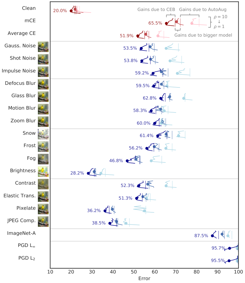
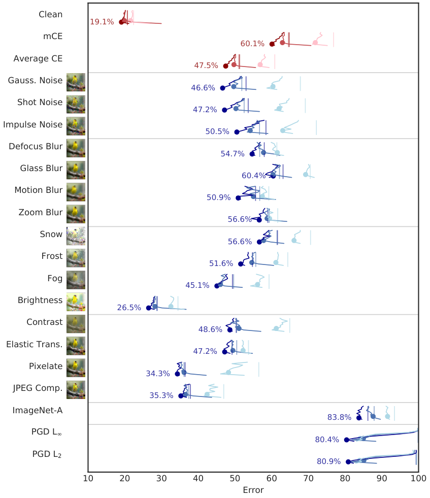
As a simple baseline we trained ResNet50 with no data augmentation using the standard cross-entropy loss (XEnt). We then trained the same network with CEB at ten different values of . AutoAug (Cubuk et al. 2018) has previously been demonstrated to improve robustness markedly on ImageNet-C, so next we trained ResNet50 with AutoAug using XEnt. We similarly trained these AutoAug ResNet50 networks using CEB at the same ten values of . ImageNet-C numbers are also sensitive to the model capacity. To assess whether CEB can benefit larger models, we repeated the experiments with a modified ResNet50 network where every layer was made twice as wide, training an XEnt model and ten CEB models, all with AutoAug. To see if there is any additional benefit or cost to using the consistent classifier (Section 2.3), we took the same wide architecture using AutoAug and trained ten consistent classifier CEB (cCEB) models. Finally, we repeated all of the previous experiments using ResNet152: XEnt and CEB models without AutoAug; with AutoAug; with AutoAug and twice as wide; and cCEB with AutoAug and twice as wide. All other hyperparameters (learning rate schedule, L2 weight decay scale, etc.) remained the same across all models. All of those hyperparameters where taken from the ResNet hyperparameters given in the AutoAug paper. In total we trained 86 ImageNet models: 6 deterministic XEnt models varying augmentation, width, and depth; 60 CEB models additionally varying ; and 20 cCEB models also varying . The results for the ResNet50 models are summarized in Figure 3. For ResNet152, see Figure 4. See Table 1 for detailed results across the matrix of experiments.
The CEB models highlighted in Figures 3 and 4 and Table 1 were selected by cross validation. These were values of that gave the best clean test set accuracy. Despite being selected for classical generalization, these models also demonstrate a high degree of robustness on both average- and worst-case perturbations. In the case that more than one model gets the same test set accuracy, we choose the model with the lower , since we know that lower correlates with higher robustness. The only model where we had to make this decision was for ResNet152 with AutoAug, where five models all were within 0.1% of each other, so we chose the model, rather than .
Accuracy, ImageNet-C, and ImageNet-A.
Increasing model capacity and using AutoAug have positive effects on classification accuracy, as well as on robustness to ImageNet-C and ImageNet-A, but for all three classes of models CEB gives substantial additional improvements. cCEB gives a small but noticeable additional gain for all three cases (except indistinguishable performance compared to CEB on ImageNet-A with the wide ResNet152 architecture), indicating that enforcing variational consistency is a reasonable modification to the CEB objective. In Table 1 we can see that CEB’s relative accuracy gains increase as the architecture gets larger, from gains of 1.2% for ResNet50 and ResNet152 without AutoAug, to 1.6% and 1.8% for the wide models with AutoAug. This indicates that even larger relative gains may be possible when using CEB to train larger architectures than those considered here.
Targeted PGD Attacks.
We tested on the random-target version of the PGD L2 and L∞ attacks (Kurakin et al. 2016a). Both attacks used , , and , which is considered to be a strong attack still (Xie et al. 2019). Model capacity makes a substantial difference to whitebox adversarial attacks. In particular, none of the ResNet-50 models perform well, with all but cCEB getting less than 1% top-1 accuracy. However, the Resnet-152 CEB models show a dramatic improvement over the XEnt model, with top-1 accuracy increasing from 0.09% to 17.09% between the XEnt baseline without AutoAug and the corresponding CEB model, a relative increase of 187 times. CEB and cCEB give increases nearly as large for the AutoAug and wide AutoAug models. Interestingly, for the PGD attacks, AutoAug was detrimental – the ResNet152 models without AutoAug were more robust than those with AutoAug. As with the accuracy results above, the relative robustness gains due to CEB increase as model capacity increases, indicating that further relative gains are possible.
4 Conclusion
The Conditional Entropy Bottleneck (CEB) provides a simple mechanism to improve robustness of image classifiers. We have shown a strong trend toward increased robustness as decreases in the standard Wide ResNet model on CIFAR10, and that this increased robustness does not come at the expense of accuracy relative to the deterministic baseline. We have shown that CEB models at a range of outperform an adversarially-trained baseline model, even on the attack the adversarial model was trained on, and have incidentally shown that the adversarially-trained model generalizes to at least one other attack less well than a deterministic baseline. Finally, we have shown that on ImageNet, CEB provides substantial gains over deterministic baselines in validation set accuracy, robustness to Common Corruptions, Natural Adversarial Examples, and targeted Projected Gradient Descent attacks. We hope these empirical demonstrations inspire further theoretical and practical study of the use of bottlenecking techniques to encourage improvements to both classical generalization and robustness.
Appendix A Experiment Details
Here we give additional technical details for the CIFAR10 and ImageNet experiments.
A.1 CIFAR10 Experiment Details
We trained all of the models using Adam (Kingma & Ba 2015) at a base learning rate of . We lowered the learning rate three times by a factor of 0.3 each time. The only additional trick to train the CIFAR10 models was to start with , anneal down to over 2 epochs, and then anneal to the target over one epoch once training exceeded a threshold of 20%. This jump-start method is inspired by experiments on VIB in Wu et al. 2019. It makes it much easier to train models at low , and appears to not negatively impact final performance.
A.2 ImageNet Experiment Details
We follow the learning rate schedule for the ResNet 50 from Cubuk et al. 2018, which has a top learning rate of 1.6, trains for 270 epochs, and drops the learning rate by a factor of 10 at 90, 180, and 240 epochs. The only difference for all of our models is that we train at a batch size of 8192 rather than 4096. Similar to the CIFAR10 models, in order to ensure that the ImageNet models train at low , we employ a simple jump-start. We start at and anneal down to the target over 12,000 steps. The first learning rate drop occurs a bit after 14,000 steps. Also similar to the CIFAR10 WRN experiments, none of the models we trained at succeeded, indicating that ResNet50 and wide ResNet50 both have insufficient capacity to fully learn ImageNet. We were able to train ResNet152 at , but only by disabling L2 weight decay and using a slightly lower learning rate. Since that involved additional hyperparameter tuning, we don’t report those results here, beyond noting that it is possible, and that those models reached top-1 accuracy around 72%.
Appendix B CEB Example Code
In Appendices B, B and B we give annotated code changes needed to make ResNet CEB models, based on the TPU-compatible ResNet implementation from the Google TensorFlow Team 2019.
[htbp]
Modifications to the model.py file.
[htbp]
Modification to the head of resnet_main.py.
[htbp]
Modifications to resnet_model_fn in resnet_main.py.
References
- Achille & Soatto (2017) Achille, A. and Soatto, S. Emergence of Invariance and Disentangling in Deep Representations. arXiv: 1706.01350, 2017. URL https://arxiv.org/abs/1706.01350.
- Achille & Soatto (2018) Achille, A. and Soatto, S. Information dropout: Learning optimal representations through noisy computation. IEEE Transactions on Pattern Analysis and Machine Intelligence, 2018.
- Alemi et al. (2017) Alemi, A. A., Fischer, I., Dillon, J. V., and Murphy, K. Deep Variational Information Bottleneck. In International Conference on Learning Representations, 2017. URL http://arxiv.org/abs/1612.00410.
- Athalye et al. (2018) Athalye, A., Carlini, N., and Wagner, D. Obfuscated gradients give a false sense of security: Circumventing defenses to adversarial examples. arXiv preprint arXiv:1802.00420, 2018.
- Baluja & Fischer (2017) Baluja, S. and Fischer, I. Adversarial transformation networks: Learning to generate adversarial examples. arXiv preprint arXiv:1703.09387, 2017.
- Carlini & Wagner (2017a) Carlini, N. and Wagner, D. Adversarial examples are not easily detected: Bypassing ten detection methods. In Proceedings of the 10th ACM Workshop on Artificial Intelligence and Security, pp. 3–14. ACM, 2017a.
- Carlini & Wagner (2017b) Carlini, N. and Wagner, D. Towards evaluating the robustness of neural networks. In 2017 IEEE Symposium on Security and Privacy (SP), pp. 39–57. IEEE, 2017b.
- Cubuk et al. (2018) Cubuk, E. D., Zoph, B., Mane, D., Vasudevan, V., and Le, Q. V. Autoaugment: Learning augmentation policies from data. arXiv preprint arXiv:1805.09501, 2018.
- Engstrom et al. (2019) Engstrom, L., Gilmer, J., Goh, G., Hendrycks, D., Ilyas, A., Madry, A., Nakano, R., Nakkiran, P., Santurkar, S., Tran, B., Tsipras, D., and Wallace, E. A discussion of ’adversarial examples are not bugs, they are features’. Distill, 2019. doi: 10.23915/distill.00019. https://distill.pub/2019/advex-bugs-discussion.
- Eykholt et al. (2017) Eykholt, K., Evtimov, I., Fernandes, E., Li, B., Rahmati, A., Xiao, C., Prakash, A., Kohno, T., and Song, D. Robust physical-world attacks on deep learning models. arXiv preprint arXiv:1707.08945, 2017.
- Fischer (2018) Fischer, I. The Conditional Entropy Bottleneck. Open Review, 2018.
- Goodfellow et al. (2015) Goodfellow, I. J., Shlens, J., and Szegedy, C. Explaining and harnessing adversarial examples. In CoRR, 2015.
- Google TensorFlow Team (2019) Google TensorFlow Team. Cloud TPU ResNet Implementation. https://github.com/tensorflow/tpu/tree/master/models/official/resnet, 2019. Accessed: 2019-09-30.
- Hendrycks & Dietterich (2019) Hendrycks, D. and Dietterich, T. Benchmarking neural network robustness to common corruptions and perturbations. arXiv preprint arXiv:1903.12261, 2019.
- Hendrycks et al. (2019) Hendrycks, D., Zhao, K., Basart, S., Steinhardt, J., and Song, D. Natural adversarial examples. arXiv preprint arXiv:1907.07174, 2019.
- Ilyas et al. (2019) Ilyas, A., Santurkar, S., Tsipras, D., Engstrom, L., Tran, B., and Madry, A. Adversarial examples are not bugs, they are features. arXiv preprint arXiv:1905.02175, 2019.
- Ioffe & Szegedy (2015) Ioffe, S. and Szegedy, C. Batch normalization: Accelerating deep network training by reducing internal covariate shift. arXiv preprint arXiv:1502.03167, 2015.
- Kingma & Ba (2015) Kingma, D. and Ba, J. Adam: A method for stochastic optimization. In International Conference on Learning Representations, 2015. URL https://arxiv.org/abs/1412.6980.
- Kurakin et al. (2016a) Kurakin, A., Goodfellow, I., and Bengio, S. Adversarial examples in the physical world. arXiv preprint arXiv:1607.02533, 2016a.
- Kurakin et al. (2016b) Kurakin, A., Goodfellow, I., and Bengio, S. Adversarial machine learning at scale. arXiv preprint arXiv:1611.01236, 2016b.
- Lopes et al. (2019) Lopes, R. G., Yin, D., Poole, B., Gilmer, J., and Cubuk, E. D. Improving robustness without sacrificing accuracy with patch gaussian augmentation. arXiv preprint arXiv:1906.02611, 2019.
- Madry et al. (2017) Madry, A., Makelov, A., Schmidt, L., Tsipras, D., and Vladu, A. Towards deep learning models resistant to adversarial attacks. arXiv preprint arXiv:1706.06083, 2017.
- Moosavi-Dezfooli et al. (2016) Moosavi-Dezfooli, S.-M., Fawzi, A., and Frossard, P. Deepfool: a simple and accurate method to fool deep neural networks. In Proceedings of the IEEE Conference on Computer Vision and Pattern Recognition, pp. 2574–2582, 2016.
- Szegedy et al. (2013) Szegedy, C., Zaremba, W., Sutskever, I., Bruna, J., Erhan, D., Goodfellow, I., and Fergus, R. Intriguing properties of neural networks. arXiv: 1312.6199, 2013. URL https://arxiv.org/abs/1312.6199.
- Szegedy et al. (2013) Szegedy, C., Zaremba, W., Sutskever, I., Bruna, J., Erhan, D., Goodfellow, I., and Fergus, R. Intriguing properties of neural networks. arXiv preprint arXiv:1312.6199, 2013.
- Tishby et al. (2000) Tishby, N., Pereira, F. C., and Bialek, W. The information bottleneck method. arXiv preprint physics/0004057, 2000.
- Tsipras et al. (2018) Tsipras, D., Santurkar, S., Engstrom, L., Turner, A., and Madry, A. Robustness may be at odds with accuracy. arXiv preprint arXiv:1805.12152, 2018.
- Wu et al. (2019) Wu, T., Fischer, I., Chuang, I., and Tegmark, M. Learnability for the information bottleneck. Uncertainty in AI, 2019.
- Xie et al. (2019) Xie, C., Wu, Y., Maaten, L. v. d., Yuille, A. L., and He, K. Feature denoising for improving adversarial robustness. In Proceedings of the IEEE Conference on Computer Vision and Pattern Recognition, pp. 501–509, 2019.
- Yin et al. (2019) Yin, D., Lopes, R. G., Shlens, J., Cubuk, E. D., and Gilmer, J. A fourier perspective on model robustness in computer vision. arXiv preprint arXiv:1906.08988, 2019.