Regularizing activations in neural networks via distribution matching with the Wasserstein metric
Abstract
Regularization and normalization have become indispensable components in training deep neural networks, resulting in faster training and improved generalization performance. We propose the projected error function regularization loss (PER) that encourages activations to follow the standard normal distribution. PER randomly projects activations onto one-dimensional space and computes the regularization loss in the projected space. PER is similar to the Pseudo-Huber loss in the projected space, thus taking advantage of both and regularization losses. Besides, PER can capture the interaction between hidden units by projection vector drawn from a unit sphere. By doing so, PER minimizes the upper bound of the Wasserstein distance of order one between an empirical distribution of activations and the standard normal distribution. To the best of the authors’ knowledge, this is the first work to regularize activations via distribution matching in the probability distribution space. We evaluate the proposed method on the image classification task and the word-level language modeling task.
1 Introduction
Training of deep neural networks is very challenging due to the vanishing and exploding gradient problem (Hochreiter 1998; Glorot & Bengio 2010), the presence of many flat regions and saddle points (Shalev-Shwartz et al. 2017), and the shattered gradient problem (Balduzzi et al. 2017). To remedy these issues, various methods for controlling hidden activations have been proposed such as normalization (Ioffe & Szegedy 2015; Huang et al. 2018), regularization (Littwin & Wolf 2018), initialization (Mishkin & Matas 2016; Zhang et al. 2019), and architecture design (He et al. 2016).
Among various techniques of controlling activations, one well-known and successful path is controlling their first and second moments. Back in the 1990s, it has been known that the neural network training can be benefited from normalizing input statistics so that samples have zero mean and identity covariance matrix (LeCun et al. 1998; Schraudolph 1998). This idea motivated batch normalization (BN) that considers hidden activations as the input to the next layer and normalizes scale and shift of the activations (Ioffe & Szegedy 2015).
Recent works show the effectiveness of different sample statistics of activations for normalization and regularization. Deecke et al. 2019 and Kalayeh & Shah 2019 normalize activations to several modes with different scales and translations. Variance constancy loss (VCL) implicitly normalizes the fourth moment by minimizing the variance of sample variances, which enables adaptive mode separation or collapse based on their prior probabilities (Littwin & Wolf 2018). BN is also extended to whiten activations (Huang et al. 2018; Huang et al. 2019), and to normalize general order of central moment in the sense of norm including and (Liao et al. 2016; Hoffer et al. 2018).
In this paper, we propose a projected error function regularization (PER) that regularizes activations in the Wasserstein probability distribution space. Specifically, PER pushes the distribution of activations to be close to the standard normal distribution. PER shares a similar strategy with previous approaches that dictates the ideal distribution of activations. Previous approaches, however, deal with single or few sample statistics of activations. On the contrary, PER regularizes the activations by matching the probability distributions, which considers different statistics simultaneously, e.g., all orders of moments and correlation between hidden units. The extensive experiments on multiple challenging tasks show the effectiveness of PER.
2 Related works
Many modern deep learning architectures employ BN as an essential building block for better performance and stable training even though its theoretical aspects of regularization and optimization are still actively investigated (Santurkar et al. 2018; Kohler et al. 2018; Bjorck et al. 2018; Yang et al. 2019). Several studies have applied the idea of BN that normalizes activations via the sample mean and the sample variance to a wide range of domains such as recurrent neural network (Lei Ba et al. 2016) and small batch size training (Wu & He 2018).
Huang et al. 2018; Huang et al. 2019 propose normalization techniques whitening the activation of each layer. This additional constraint on the statistical relationship between activations improves the generalization performance of residual networks compared to BN. Although the correlation between activations are not explicitly considered, dropout prevents activations from being activated at the same time, called co-adaptation, by randomly dropping the activations (Srivastava et al. 2014), the weights (Wan et al. 2013), and the spatially connected activations (Ghiasi et al. 2018).
Considering BN as the normalization in the space, several works extend BN to other spaces, i.e., other norms. Streaming normalization (Liao et al. 2016) explores the normalization of a different order of central moment with norm for general . Similarly, Hoffer et al. 2018 explores and normalization, which enable low precision computation. Littwin & Wolf 2018 proposes a regularization loss that reduces the variance of sample variances of activation that is closely related to the fourth moment.
The idea of controlling activations via statistical characteristics of activations also has motivated initialization methods. An example includes balancing variances of each layer (Glorot & Bengio 2010; He et al. 2015), bounding scale of activation and gradient (Mishkin & Matas 2016; Balduzzi et al. 2017; Gehring et al. 2017; Zhang et al. 2019), and norm preserving (Saxe et al. 2013). Although the desired initial state may not be maintained during training, experimental results show that they can stabilize the learning process as well.
Recently, the Wasserstein metric has gained much popularity in a wide range of applications in deep learning with some nice properties such as being a metric in a probability distribution space without requiring common supports of two distributions. For instance, it is successfully applied to a multi-labeled classification (Frogner et al. 2015), gradient flow of policy update in reinforcement learning (Zhang et al. 2018), training of generative models (Arjovsky et al. 2017; Gulrajani et al. 2017; Kolouri et al. 2019), and capturing long term semantic structure in sequence-to-sequence language model (Chen et al. 2019).


While the statistics such as mean and (co)variance are useful summaries of a probability distribution, they cannot fully represent the underlying structure of the distribution (Fig. 1). Therefore, regularizing or normalizing activation to follow the target distribution via statistics can be ineffective in some cases. For instance, normalizing activations via single mean and variance such as BN and decorrelated BN (Huang et al. 2018) can be inadequate in learning multimodal distribution (Bilen & Vedaldi 2017; Deecke et al. 2019). This limitation motivates us to investigate a more general way of regularizing the distribution of activations. Instead of controlling activations via statistics, we define the target distribution and then minimize the Wasserstein distance between the activation distribution and the target distribution.
3 Projected error function regularization
We consider a neural network with layers each of which has hidden units in layer . Let be training samples which are assumed to be i.i.d. samples drawn from a probability distribution . In this paper, we consider the optimization by stochastic gradient descent with mini-batch of samples randomly drawn from at each training iteration. For -th element of the samples, the neural network recursively computes:
| (1) |
where , is an activation in layer , and is an activation function. In the case of recurrent neural networks (RNNs), the recursive relationship takes the form of:
| (2) |
where is an activation in layer at time and is an initial state. Without loss of generality, we focus on activations in layer of feed-forward networks and the mini-batch of samples . Throughout this paper, we let be a function made by compositions of recurrent relation in equation 1 up to layer , i.e., , and be a -th output of .
This paper proposes a new regularization loss, called projected error function regularization (PER), that encourages activations to follow the standard normal distribution. Specifically, PER directly matches the distribution of activations to the target distribution via the Wasserstein metric. Let be the Gaussian measure defined as and be the empirical measure of hidden activations where is the Dirac unit mass on . Then, the Wasserstein metric of order between and is defined by:
| (3) |
where is the set of all joint probability measures on having the first and the second marginals and , respectively.
Because direct computation of equation 3 is intractable, we consider the sliced Wasserstein distance (Rabin et al. 2011) approximating the Wasserstein distance by projecting the high dimensional distributions onto (Fig. 2). It is proved by that the sliced Wasserstein and the Wasserstein are equivalent metrics (Santambrogio 2015; Bonnotte 2013). The sliced Wasserstein of order one between and can be formulated as:
| (4) |
where is a unit sphere in , and represent the measures projected to the angle , is a uniform measure on , and is a cumulative distribution function of . Herein, equation 4 can be evaluated through sorting for each angle .
While we can directly use the sliced Wasserstein in equation 4 as a regularization loss, it has a computational dependency on the batch dimension due to the sorting. The computational dependency between samples may not be desirable in distributed and large-batch training that is becoming more and more prevalent in recent years. For this reason, we remove the dependency by applying the Minkowski inequality to equation 4, and obtain the regularization loss :
| (5) |
whose gradient with respect to is:
| (6) |
where is the uniform distribution on . In this paper, expectation over is approximated by the Monte Carlo method with number of samples. Therefore, PER results in simple modification of the backward pass as in Alg. 1.
Input The number of Monte Carlo evaluations , an activation for -th sample , the gradient of the loss , a regularization coefficient
Encouraging activations to follow the standard normal distribution can be motivated by the natural gradient (Amari 1998). The natural gradient is the steepest descent direction in a Riemannian manifold, and it is also the direction that maximizes the probability of not increasing generalization error (Roux et al. 2008). The natural gradient is obtained by multiplying the inverse Fisher information matrix to the gradient. In Raiko et al. 2012 and Desjardins et al. 2015, under the independence assumption between forward and backward passes and activations between different layers, the Fisher information matrix is a block diagonal matrix each of which block is given by:
| (7) |
where is vectorized , , and for .
Since computing the inverse Fisher information matrix is too expensive to perform every iterations, previous studies put efforts into developing reparametrization techniques, activation functions, and regularization losses to make close to , thereby making the gradient close to the natural gradient. For instance, making zero mean and unit variance activations (LeCun et al. 1998; Schraudolph 1998; Glorot & Bengio 2010; Raiko et al. 2012; Wiesler et al. 2014) and decorrelated activations (Cogswell et al. 2016; Xiong et al. 2016; Huang et al. 2018) make , and these techniques result in faster training and improved generalization performance. In this perspective, it is expected that PER will enjoy the same advantages by matching to .
3.1 Comparison to controlling activations in space
In this subsection, we theoretically compare PER with existing methods that control activations in space. is the space of measurable functions whose -th power of absolute value is Lebesgue integrable, and norm of is given by:
| (8) |
where is the unknown probability distribution generating training samples . Since we have no access to , it is approximated by the empirical measure of mini-batch samples.
The norm is widely used in the literature for regularization and normalization of neural networks. For instance, activation norm regularization (Merity et al. 2017a) penalizes norm of activations. As another example, BN and its -th order generalization use norm such that the norm of the centralized activation, or pre-activation, is bounded:
| (9) |
where is -th unit of , is the sample mean, is a learnable shift parameter, and is a learnable scale parameters. Herein, we have for any unit and any empirical measure, thus .

PER differs from norm-based approaches in two aspects. First, PER can be considered as norm with adaptive order in the projected space because it is very similar to the Pseudo-Huber loss in one-dimensional space (Fig. 3). Herein, the Pseudo-Huber loss is a smooth approximation of the Huber loss (Huber 1964). Therefore, PER smoothly changes its behavior between and norms, making the regularization loss sensitive to small values and insensitive to outliers with large values. However, the previous approaches use predetermined order , which makes the norm to change insensitively in the near-zero region when or to explode in large value region when .
Second, PER captures the interaction between hidden units by projection vectors, unlike norm. To see this, let where is the natural basis of . That is, the norm computes the regularization loss, or the normalizer, of activations with the natural basis as a projection vector. However, PER uses general projection vectors , capturing the interaction between hidden units when computing the regularization loss. These two differences make PER more delicate criterion for regularizing activations in deep neural networks than norm, as we will show in the next section.
4 Experiments
This section illustrates the effectiveness of PER through experiments on different benchmark tasks with various datasets and architectures. We compare PER with BN normalizing the first and second moments and VCL regularizing the fourth moments. PER is also compared with and activation norm regularizations that behave similarly in some regions of the projected space. We then analyze the computational complexity PER and the impact of PER on the distribution of activations. Throughout all experiments, we use 256 number of slices and the same regularization coefficient for the regularization losses computed in each layer.
4.1 Image classification in CIFAR-10, CIFAR-100, and tiny ImageNet
We evaluate PER in image classification task in CIFAR (Krizhevsky et al. 2009) and a subset of ImageNet (Russakovsky et al. 2015), called tiny ImageNet. We first evaluate PER with ResNet (He et al. 2016) in CIFAR-10 and compare it with BN and a vanilla network initialized by fixup initialization (Zhang et al. 2019). We match the experimental details in training under BN with He et al. 2016 and under PER and vanilla with Zhang et al. 2019, and we obtain similar performances presented in the papers. Herein, we search the regularization coefficient over { 3e-4, 1e-4, 3e-5, 1e-5 }. Table 2 presents results of CIFAR-10 experiments with ResNet-56 and ResNet-110. PER outperforms BN as well as vanilla networks in both architectures. Especially, PER improves the test errors by 0.49 and 0.71 in ResNet-56 and ResNet-110 without BN, respectively.
| Model | Method | Test error |
|---|---|---|
| ResNet-56 | Vanilla | 7.21 |
| BN | 6.95 | |
| PER | 6.72 | |
| ResNet-110 | Vanilla | 6.90 (7.24*) |
| BN | 6.62 (6.61**) | |
| PER | 6.19 |
| Method | Test error |
|---|---|
| Vanilla | 37.45 (39.22) |
| BN | 39.22 (40.02) |
| VCL | (37.30) |
| PER | 36.74 |
We also performed experiments on an 11-layer convolutional neural network (11-layer CNN) examined in VCL (Littwin & Wolf 2018). This architecture is originally proposed in Clevert et al. 2016. Following Littwin & Wolf 2018, we perform experiments on 11-layer CNNs with ELU, ReLU, and Leaky ReLU activations, and match experimental details in Littwin & Wolf 2018 except that we used 10x less learning rate for bias parameters and additional scalar bias after ReLU and Leaky ReLU based on Zhang et al. 2019. By doing so, we obtain similar results presented in Littwin & Wolf 2018. Again, a search space of the regularization coefficient is { 3e-4, 1e-4, 3e-5, 1e-5 }. For ReLU and Leaky ReLU in CIFAR-100, however, we additionally search { 3e-6, 1e-6, 3e-7, 1e-7 } because of divergence of training with PER in these setting. As shown in Table 3, PER shows the best performances on four out of six experiments. In other cases, PER gives compatible performances to BN or VCL, giving 0.16 % less than the best performances.
| Activation | Method | CIFAR-10 | CIFAR-100 |
|---|---|---|---|
| ReLU | Vanilla | (8.36) | (32.80) |
| BN | (7.78) | 29.13 (29.10) | |
| VCL | (7.80) | (30.30) | |
| PER | 7.21 | 29.29 | |
| LeakyReLU | Vanilla | (6.70) | (26.80) |
| BN | (7.08) | (27.20) | |
| VCL | (6.45) | (26.30) | |
| PER | 6.29 | 25.50 | |
| ELU | Vanilla | (6.98) | (28.70) |
| BN | (6.63) | (26.90) | |
| VCL | 6.26 (6.15) | (25.60) | |
| PER | 6.42 | 25.73 |
Following Littwin & Wolf 2018, PER is also evaluated on tiny ImageNet. In this experiment, the number of convolutional filters in each layer is doubled. Due to the limited time and resources, we conduct experiments only with ELU that gives good performances for PER, BN, and VCL in CIFAR. As shown in Table 2, PER is also effective in the larger model in the larger image classification dataset.
4.2 Language modeling in PTB and WikiText2
We evaluate PER in word-level language modeling task in PTB (Mikolov et al. 2010) and WikiText2 (Merity et al. 2017b). We apply PER to LSTM with two layers having 650 hidden units with and without reuse embedding (RE) proposed in Inan et al. 2017 and Press & Wolf 2016, and variational dropout (VD) proposed in Gal & Ghahramani 2016. We used the same configurations with Merity et al. 2017a and failed to reproduce the results in Merity et al. 2017a. Especially, when we rescale gradient when its norm exceeds 10, we observed divergence or bad performance (almost 2x perplexity compared to the published result). Therefore, we rescale gradient with norm over 0.25 instead of 10 based on the default hyperparameter of the PyTorch word-level language model11 1 Available in https://github.com/pytorch/examples/tree/master/word_language_model that is also mentioned in Merity et al. 2017a. We also train the networks for 60 epochs instead of 80 epochs since validation perplexity is not improved after 60 epochs in most cases. In this task, PER is compared with recurrent BN (RBN; Cooijmans et al. 2017, Cooijmans et al. 2017) because BN is not directly applicable to LSTM. We also compare PER with and activation norm regularizations. Herein, the search space of regularization coefficients of PER, regularization, and regularization is {3e-4, 1e-4, 3e-5 }. For and penalties in PTB, we search additional coefficients over { 1e-5, 3e-6, 1e-6, 3e-6, 1e-6, 3e-7, 1e-7 } because the searched coefficients seem to constrain the capacity.
We list in Table 4 the perplexities of methods on PTB and WikiText2. While all regularization techniques show regularization effects by giving improved test perplexity, PER gives the best test perplexity except LSTM and RE-VD-LSTM in the PTB dataset wherein PER is the second-best method. We also note that naively applying RBN often reduces performance. For instance, RBN increases test perplexity of VD-LSTM by about 5 in PTB and WikiText2.
| PTB | WikiText2 | ||||
|---|---|---|---|---|---|
| Model | Method | Valid | Test | Valid | Test |
| LSTM | Vanilla | 123.2 | 122.0 | 138.9 | 132.7 |
| penalty | 119.6 | 114.1 | 137.7 | 130.0 | |
| penalty | 120.5 | 115.2 | 136.0 | 131.1 | |
| RBN | 118.2 | 115.1 | 156.2 | 148.3 | |
| PER | 118.5 | 114.5 | 134.2 | 129.6 | |
| RE-LSTM | Vanilla | 114.1 | 112.2 | 129.2 | 123.2 |
| penalty | 112.2 | 108.5 | 128.6 | 122.7 | |
| penalty | 116.6 | 108.2 | 126.5 | 123.3 | |
| RBN | 113.6 | 110.4 | 138.1 | 131.6 | |
| PER | 110.0 | 108.5 | 123.2 | 117.4 | |
| VD-LSTM | Vanilla | 84.9 | 81.1 | 99.6 | 94.5 |
| penalty | 84.9 | 81.5 | 98.2 | 92.9 | |
| penalty | 84.5 | 81.2 | 98.8 | 94.2 | |
| RBN | 89.7 | 86.4 | 104.3 | 99.4 | |
| PER | 84.1 | 80.7 | 98.1 | 92.6 | |
| RE-VD-LSTM | Vanilla | 78.9 | 75.7 | 91.4 | 86.4 |
| penalty | 78.3 | 75.1 | 90.5 | 86.1 | |
| penalty | 79.2 | 75.8 | 90.3 | 86.1 | |
| RBN | 83.7 | 80.5 | 95.5 | 90.5 | |
| PER | 78.1 | 74.9 | 90.6 | 85.9 | |
4.3 Analysis
In this subsection, we analyze the computational complexity of PER and its impact on closeness to the standard normal distribution in the 11-layer CNN.
4.3.1 Computational complexity
PER has no additional parameters. However, BN and VCL require additional parameters for each channel and each location and channel in every layer, respectively; that is, 2.5K and 350K number of parameters are introduced in BN and VCL in the 11-layer CNN, respectively. In terms of time complexity, PER has the complexity of for projection operation in each layer . On the other hand, BN and VCL have complexities. In our benchmarking, each training iteration takes 0.071 seconds for a vanilla network, 0.083 seconds for BN, 0.087 for VCL, and 0.093 seconds for PER on a single NVIDIA TITAN X. Even though PER requires slightly more training time than BN and VCL, this disadvantage can be mitigated by computation of PER is only required in training and PER does not have additional parameters.
4.3.2 Closeness to the standard normal distribution
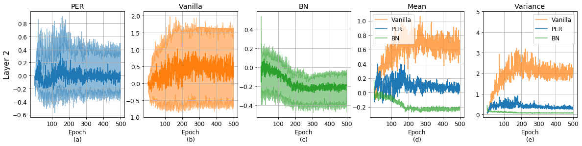
To examine the effect of PER on the closeness to , we analyze the distribution of activations in 11-layer CNN in different perspectives. We first analyze the distribution of a single activation for some unit and layer (Fig. 4). We observe that changes in probability distributions between two consecutive epochs are small under BN because BN bound the norm of activations into learned parameters. On the contrary, activation distributions under vanilla and PER are jiggled between two consecutive epochs. However, PER prevents the variance explosion and pushes the mean to zero. As shown in Fig. 4, while variances of under both PER and Vanilla are very high at the beginning of training, the variance keeps moving towards one under PER during training. Similarly, PER recovers biased means of and at the early stage of learning.
To precisely evaluate closeness to the standard normal distribution, we also analyze at each epoch (Fig. 5). Herein, the sliced Wasserstein distance is computed by approximating the Gaussian measure using the empirical measure of samples drawn from as in Rabin et al. 2011. As similar to the previous result, while BN and at initial state gives small in early stage of training, PER also can effectively control the distribution without such normalization. This confirms that PER prevents the distribution of activation to be drifted away from the target distribution.


5 Conclusion
We proposed the regularization loss that minimizes the upper bound of the 1-Wasserstein distance between the standard normal distribution and the distribution of activations. In image classification and language modeling experiments, PER gives marginal but consistent improvements over methods based on sample statistics (BN and VCL) as well as and activation regularization methods. The analysis of changes in activations’ distribution during training verifies that PER can stabilize the probability distribution of activations without normalization. Considering that the regularization loss can be easily applied to a wide range of tasks without changing architectures or training strategies unlike BN, we believe that the results indicate the valuable potential of regularizing networks in the probability distribution space as a future direction of research.
The idea of regularizing activations with the metric in probability distribution space can be extended to many useful applications. For instance, one can utilize task-specific prior when determining a target distribution, e.g., the Laplace distribution for making sparse activation. The empirical distribution of activations computed by a pretrained network can also be used as a target distribution to prevent catastrophic forgetting. In this case, the activation distribution can be regularized so that it does not drift away from the activation distribution learned in the previous task as different from previous approaches constrains the changes in the the function space of logits (Benjamin et al. 2019).
Acknowledgments
We would like to thank Min-Gwan Seo, Dong-Hyun Lee, Dongmin Shin, and anonymous reviewers for the discussions and suggestions.
References
- Amari (1998) Shun-Ichi Amari. Natural gradient works efficiently in learning. Neural Computation, 10(2):251–276, 1998.
- Arjovsky et al. (2017) Martin Arjovsky, Soumith Chintala, and Léon Bottou. Wasserstein generative adversarial networks. In International Conference on Machine Learning, 2017.
- Balduzzi et al. (2017) David Balduzzi, Marcus Frean, Lennox Leary, JP Lewis, Kurt Wan-Duo Ma, and Brian McWilliams. The shattered gradients problem: If resnets are the answer, then what is the question? In International Conference on Machine Learning, 2017.
- Benjamin et al. (2019) Ari S Benjamin, David Rolnick, and Konrad Kording. Measuring and regularizing networks in function space. In International Conference on Learning Representations, 2019.
- Bilen & Vedaldi (2017) Hakan Bilen and Andrea Vedaldi. Universal representations: The missing link between faces, text, planktons, and cat breeds. arXiv preprint arXiv:1701.07275, 2017.
- Bjorck et al. (2018) Nils Bjorck, Carla P Gomes, Bart Selman, and Kilian Q Weinberger. Understanding batch normalization. In Advances in Neural Information Processing Systems, 2018.
- Bonnotte (2013) Nicolas Bonnotte. Unidimensional and Evolution Methods for Optimal Transportation. PhD thesis, Paris 11, 2013.
- Chen et al. (2019) Liqun Chen, Yizhe Zhang, Ruiyi Zhang, Chenyang Tao, Zhe Gan, Haichao Zhang, Bai Li, Dinghan Shen, Changyou Chen, and Lawrence Carin. Improving sequence-to-sequence learning via optimal transport. In International Conference on Learning Representations, 2019.
- Clevert et al. (2016) Djork-Arné Clevert, Thomas Unterthiner, and Sepp Hochreiter. Fast and accurate deep network learning by exponential linear units (ELUs). In International Conference of Learning Representations, 2016.
- Cogswell et al. (2016) Michael Cogswell, Faruk Ahmed, Ross Girshick, Larry Zitnick, and Dhruv Batra. Reducing overfitting in deep networks by decorrelating representations. In International Conference on Learning Representations, 2016.
- Cooijmans et al. (2017) Tim Cooijmans, Nicolas Ballas, César Laurent, Çağlar Gülçehre, and Aaron Courville. Recurrent batch normalization. In International Conference on Learning Representations, 2017.
- Deecke et al. (2019) Lucas Deecke, Iain Murray, and Hakan Bilen. Mode normalization. In International Conference on Learning Representations, 2019.
- Desjardins et al. (2015) Guillaume Desjardins, Karen Simonyan, Razvan Pascanu, et al. Natural neural networks. In Advances in Neural Information Processing Systems, 2015.
- Frogner et al. (2015) Charlie Frogner, Chiyuan Zhang, Hossein Mobahi, Mauricio Araya, and Tomaso A Poggio. Learning with a Wasserstein loss. In Advances in Neural Information Processing Systems, 2015.
- Gal & Ghahramani (2016) Yarin Gal and Zoubin Ghahramani. A theoretically grounded application of dropout in recurrent neural networks. In Advances in Neural Information Processing Systems, 2016.
- Gehring et al. (2017) Jonas Gehring, Michael Auli, David Grangier, Denis Yarats, and Yann N Dauphin. Convolutional sequence to sequence learning. In International Conference on Machine Learning, 2017.
- Ghiasi et al. (2018) Golnaz Ghiasi, Tsung-Yi Lin, and Quoc V Le. Dropblock: A regularization method for convolutional networks. In Advances in Neural Information Processing Systems, 2018.
- Glorot & Bengio (2010) Xavier Glorot and Yoshua Bengio. Understanding the difficulty of training deep feedforward neural networks. In Artificial Intelligence and Statistics, 2010.
- Gulrajani et al. (2017) Ishaan Gulrajani, Faruk Ahmed, Martin Arjovsky, Vincent Dumoulin, and Aaron C Courville. Improved training of Wasserstein gans. In Advances in Neural Information Processing Systems, 2017.
- He et al. (2015) Kaiming He, Xiangyu Zhang, Shaoqing Ren, and Jian Sun. Delving deep into rectifiers: Surpassing human-level performance on imagenet classification. In IEEE International Conference on Computer Vision, 2015.
- He et al. (2016) Kaiming He, Xiangyu Zhang, Shaoqing Ren, and Jian Sun. Deep residual learning for image recognition. In IEEE Conference on Computer Vision and Pattern Recognition, 2016.
- Hochreiter (1998) Sepp Hochreiter. The vanishing gradient problem during learning recurrent neural nets and problem solutions. International Journal of Uncertainty, Fuzziness and Knowledge-Based Systems, 6(02):107–116, 1998.
- Hoffer et al. (2018) Elad Hoffer, Ron Banner, Itay Golan, and Daniel Soudry. Norm matters: Efficient and accurate normalization schemes in deep networks. In Advances in Neural Information Processing Systems, 2018.
- Huang et al. (2018) Lei Huang, Dawei Yang, Bo Lang, and Jia Deng. Decorrelated batch normalization. In IEEE Conference on Computer Vision and Pattern Recognition, 2018.
- Huang et al. (2019) Lei Huang, Yi Zhou, Fan Zhu, Li Liu, and Ling Shao. Iterative normalization: Beyond standardization towards efficient whitening. In IEEE Conference on Computer Vision and Pattern Recognition, 2019.
- Huber (1964) Peter J Huber. Robust estimation of a location parameter. The Annals of Mathematical Statistics, pp. 73–101, 1964.
- Inan et al. (2017) Hakan Inan, Khashayar Khosravi, and Richard Socher. Tying word vectors and word classifiers: A loss framework for language modeling. In International Conference on Learning Representations, 2017.
- Ioffe & Szegedy (2015) Sergey Ioffe and Christian Szegedy. Batch normalization: Accelerating deep network training by reducing internal covariate shift. In International Conference on Machine Learning, 2015.
- Kalayeh & Shah (2019) Mahdi M Kalayeh and Mubarak Shah. Training faster by separating modes of variation in batch-normalized models. IEEE Transactions on Pattern Analysis and Machine Intelligence, 2019.
- Kohler et al. (2018) Jonas Kohler, Hadi Daneshmand, Aurelien Lucchi, Ming Zhou, Klaus Neymeyr, and Thomas Hofmann. Towards a theoretical understanding of batch normalization. arXiv preprint arXiv:1805.10694, 2018.
- Kolouri et al. (2019) Soheil Kolouri, Phillip E. Pope, Charles E. Martin, and Gustavo K. Rohde. Sliced Wasserstein auto-encoders. In International Conference on Learning Representations, 2019.
- Krizhevsky et al. (2009) Alex Krizhevsky, Geoffrey Hinton, et al. Learning multiple layers of features from tiny images. Technical report, 2009.
- LeCun et al. (1998) Yann LeCun, Leon Bottou, Genevieve B Orr, and Klaus-Robert Müller. Efficient backprop. In Neural Networks: Tricks of the Trade, pp. 9–50. 1998.
- Lei Ba et al. (2016) Jimmy Lei Ba, Jamie Ryan Kiros, and Geoffrey E Hinton. Layer normalization. arXiv preprint arXiv:1607.06450, 2016.
- Liao et al. (2016) Qianli Liao, Kenji Kawaguchi, and Tomaso Poggio. Streaming normalization: Towards simpler and more biologically-plausible normalizations for online and recurrent learning. arXiv preprint arXiv:1610.06160, 2016.
- Littwin & Wolf (2018) Etai Littwin and Lior Wolf. Regularizing by the variance of the activations’ sample-variances. In Advances in Neural Information Processing Systems, 2018.
- Merity et al. (2017a) Stephen Merity, Bryan McCann, and Richard Socher. Revisiting activation regularization for language rnns. In International Conference on Machine Learning, 2017a.
- Merity et al. (2017b) Stephen Merity, Caiming Xiong, James Bradbury, and Richard Socher. Pointer sentinel mixture models. In International Conference on Learning Representations, 2017b.
- Mikolov et al. (2010) Tomáš Mikolov, Martin Karafiát, Lukáš Burget, Jan Černockỳ, and Sanjeev Khudanpur. Recurrent neural network based language model. In Annual Conference of the International Speech Communication Association, 2010.
- Mishkin & Matas (2016) Dmytro Mishkin and Jiri Matas. All you need is a good init. In International Conference on Learning Representations, 2016.
- Press & Wolf (2016) Ofir Press and Lior Wolf. Using the output embedding to improve language models. arXiv preprint arXiv:1608.05859, 2016.
- Rabin et al. (2011) Julien Rabin, Gabriel Peyré, Julie Delon, and Marc Bernot. Wasserstein barycenter and its application to texture mixing. In International Conference on Scale Space and Variational Methods in Computer Vision, 2011.
- Raiko et al. (2012) Tapani Raiko, Harri Valpola, and Yann LeCun. Deep learning made easier by linear transformations in perceptrons. In Artificial Intelligence and Statistics, 2012.
- Roux et al. (2008) Nicolas L Roux, Pierre-Antoine Manzagol, and Yoshua Bengio. Topmoumoute online natural gradient algorithm. In Advances in Neural Information Processing Systems, 2008.
- Russakovsky et al. (2015) Olga Russakovsky, Jia Deng, Hao Su, Jonathan Krause, Sanjeev Satheesh, Sean Ma, Zhiheng Huang, Andrej Karpathy, Aditya Khosla, Michael Bernstein, Alexander C. Berg, and Li Fei-Fei. ImageNet large scale visual recognition challenge. International Journal of Computer Vision, 115(3):211–252, 2015.
- Santambrogio (2015) Filippo Santambrogio. Optimal transport for applied mathematicians. Birkäuser, NY, 55:58–63, 2015.
- Santurkar et al. (2018) Shibani Santurkar, Dimitris Tsipras, Andrew Ilyas, and Aleksander Madry. How does batch normalization help optimization? In Advances in Neural Information Processing Systems, 2018.
- Saxe et al. (2013) Andrew M Saxe, James L McClelland, and Surya Ganguli. Exact solutions to the nonlinear dynamics of learning in deep linear neural networks. arXiv preprint arXiv:1312.6120, 2013.
- Schraudolph (1998) Nicol Schraudolph. Accelerated gradient descent by factor-centering decomposition. Technical report, 1998.
- Shalev-Shwartz et al. (2017) Shai Shalev-Shwartz, Ohad Shamir, and Shaked Shammah. Failures of gradient-based deep learning. In International Conference on Machine Learning, 2017.
- Srivastava et al. (2014) Nitish Srivastava, Geoffrey Hinton, Alex Krizhevsky, Ilya Sutskever, and Ruslan Salakhutdinov. Dropout: A simple way to prevent neural networks from overfitting. Journal of Machine Learning Research, 15(1):1929–1958, 2014.
- Wan et al. (2013) Li Wan, Matthew Zeiler, Sixin Zhang, Yann Le Cun, and Rob Fergus. Regularization of neural networks using dropconnect. In International Conference on Machine Learning, 2013.
- Wiesler et al. (2014) Simon Wiesler, Alexander Richard, Ralf Schlüter, and Hermann Ney. Mean-normalized stochastic gradient for large-scale deep learning. In IEEE International Conference on Acoustics, Speech and Signal Processing, 2014.
- Wu & He (2018) Yuxin Wu and Kaiming He. Group normalization. In European Conference on Computer Vision, 2018.
- Xiong et al. (2016) Wei Xiong, Bo Du, Lefei Zhang, Ruimin Hu, and Dacheng Tao. Regularizing deep convolutional neural networks with a structured decorrelation constraint. In IEEE International Conference on Data Mining, 2016.
- Yang et al. (2019) Greg Yang, Jeffrey Pennington, Vinay Rao, Jascha Sohl-Dickstein, and Samuel S Schoenholz. A mean field theory of batch normalization. In International Conference on Learning Representations, 2019.
- Zhang et al. (2019) Hongyi Zhang, Yann N Dauphin, and Tengyu Ma. Fixup initialization: Residual learning without normalization. In International Conference on Learning Representations, 2019.
- Zhang et al. (2018) Ruiyi Zhang, Changyou Chen, Chunyuan Li, and Lawrence Carin. Policy optimization as Wasserstein gradient flows. In International Conference on Machine Learning, 2018.