Generalised Hermite Spectral Methods for PDEs involving integral fractional Laplacian and Schrödinger operatorsThanks: ¹Division of Mathematical Sciences, School of Physical and Mathematical Sciences, Nanyang Technological University, 637371, Singapore. The research of the authors is partially supported by Singapore MOE AcRF Tier 2 Grants: MOE2018-T2-1-059 and MOE2017-T2-2-144. Emails: ctsheng@ntu.edu.sg (C. Sheng) and lilian@ntu.edu.sg (L. Wang).
²School of Mathematical Sciences, Peking University, Beijing 100871, China. Email: masuna@csrc.ac.cn (S. Ma).
³State Key Laboratory of Computer Science/Laboratory of Parallel Computing, Institute of Software, Chinese Academy of Sciences, Beijing 100190, China. The work of this author is partially supported by the National Natural Science Foundation of China (No. 11871455 and 11971016). Email: huiyuan@iscas.ac.cn (H. Li).
⁴Beijing Computational Science Research Center, Beijing, 100193, P.R. China. The research of this author is supported in part by the National Natural Science Foundation of China (NSFC 11871092 and NSAF U1930402). Email: lljia@csrc.ac.cn (L. Jia).

Changtao Sheng¹, Suna Ma

{}^{2},

Huiyuan Li³, Li-Lian Wang¹ and Lueling Jia⁴

Abstract.

In this paper, we introduce two new families of generalised Hermite polynomials/functions (GHPs/GHFs) in arbitrary dimensions, and develop efficient and accurate generalised Hermite spectral algorithms for PDEs with integral fractional Laplacian (IFL) and/or Schrödinger operators in $\mathbb{R}^{d}.$ As a generalisation of the G. Szegö’s family in 1D (1939), the first family of GHPs (resp. GHFs) are orthogonal with respect to $|\bm{x}|^{2\mu}\mathrm{e}^{-|\bm{x}|^{2}}$ (resp. $|\bm{x}|^{2\mu}$ ) in $\mathbb{R}^{d}$ . We further define adjoint generalised Hermite functions (A-GHFs) which have an interwoven connection with the corresponding GHFs through the Fourier transform, and which are orthogonal with respect to the inner product $[u,v]_{H^{s}(\mathbb{R}^{d})}=((-\Delta)^{s/2}u,(-\Delta)^{s/2}v)_{\mathbb{R}^{d}}$ associated with the IFL of order $s>0$ . Thus, the spectral-Galerkin method using A-GHFs as basis functions leads to a diagonal stiffness matrix for the IFL (which is known to be notoriously difficult and expensive to discretise). The new basis also finds efficient and accurate in solving PDEs with the fractional Schrödinger operator: $(-\Delta)^{s}+|\bm{x}|^{2\mu}$ with $s\in(0,1]$ and $\mu>-1/2.$ Following the same spirit, we construct the second family of GHFs, dubbed as Müntz-type generalised Hermite functions (M-GHFs), which are orthogonal with respect to an inner product associated with the underlying Schrödinger operator, and are tailored to the singularity of the solution at the origin. We demonstrate that the Müntz-type GHF spectral method leads to sparse matrices and spectrally accurate to some Schrödinger eigenvalue problems.

Key words and phrases:

Generalised Hermite polynomials/functions, integral fractional Laplacian, Schrödinger operators with fractional power potential, Müntz-type generalised Hermite functions.

2000 Mathematics Subject Classification

65N35, 65N25, 35Q40, 33C45, 65M70.

1. Introduction

In the seminal monograph [37, P. 371] (1939), Szegö first introduced a generalisation of the Hermite polynomials (denoted by $H^{(\mu)}_{n}(x),\,\mu>-1/2,\,x\in\mathbb{R}:=(-\infty,\infty)$ and dubbed as generalised Hermite polynomials (GHPs)), through an explicit second-order differential equation in an exercise problem. The GHPs defined therein are orthogonal with respect to the weight function $|x|^{2\mu}\mathrm{e}^{-x^{2}}$ . Chihara perhaps was among the first who systematically studied the properties of the GHPs, and the associated generalised Hermite functions (GHFs): $\widehat{H}^{(\mu)}_{n}(x):=\mathrm{e}^{-x^{2}/2}H^{(\mu)}_{n}(x)$ (orthogonal with respect to the weight function $|x|^{2\mu}$ ), in his PhD thesis [9, entitled as “Generalised Hermite Polynomials”] (1955). Later, some standard properties were collected in his book [10] (1978). Whereas the usual Hermite polynomials/functions are well-studied especially in spectral approximations, there have been very limited works on this generalised family (see, e.g., [30, 28, 29, 23] for the properties or further generalisations). Indeed, to the best of our knowledge, the generalised Hermite spectral methods in both theory and applications are still under-explored, and worthy of deep investigation.

The main purpose of this paper is to introduce two new families of GHPs/GHFs in arbitrary spatial dimensions, and explore their applications in solutions of PDEs involving the integral fractional Laplacian and/or Schrödinger operators.

Firstly, we construct the $d$ -dimensional GHPs $\{H_{k,\ell}^{\mu,n}(\bm{x})\}$ (cf. (2.12)) and GHFs $\{\widehat{H}_{k,\ell}^{\mu,n}(\bm{x})\}$ (cf. (2.13)), which are orthogonal with respect to the weight functions $|\bm{x}|^{2\mu}\mathrm{e}^{-|\bm{x}|^{2}}$ and $|\bm{x}|^{2\mu}$ in $\mathbb{R}^{d}$ with $\mu>-\frac{1}{2},$ respectively. In one dimension, they reduce to Szegö’s GHPs/GHFs (up to a constant multiple). More importantly, we introduce for the first time a family of adjoint generalised Hermite functions (A-GHFs) $\{\widecheck{H}^{\mu,n}_{k,\ell}(\bm{x})\}$ (cf. (2.27)) with some appealing properties. For example, this adjoint pair is closely interwoven through the Fourier transform

\mathscr{F}[\widehat{H}_{k,\ell}^{\mu,n}](\bm{\xi})=\mathrm{i}^{n+2k}\widecheck{H}_{k,\ell}^{\mu,n}(\bm{\xi}),\quad\mathscr{F}[\widecheck{H}_{k,\ell}^{\mu,n}](\bm{\xi})=(-\mathrm{i})^{n+2k}\widehat{H}_{k,\ell}^{\mu,n}(\bm{\xi}).

(1.1)

More notably, the A-GHFs are orthogonal with respect to the inner product that induces the so-called Gagliardo semi-norm of the fractional Sobolev space $H^{s}(\mathbb{R}^{d})$ for $s\in(0,1],$ that is,

[\widecheck{H}_{k,\ell}^{s,n},\widecheck{H}_{j,\iota}^{s,m}]_{H^{s}(\mathbb{R}^{d})}=\big((-\Delta)^{\frac{s}{2}}\widecheck{H}_{k,\ell}^{s,n},(-\Delta)^{\frac{s}{2}}\widecheck{H}_{j,\iota}^{s,m}\big)_{\mathbb{R}^{d}}=\delta_{jk}\delta_{mn}\delta_{\ell\iota},

(1.2)

where $(-\Delta)^{s}$ is the integral fractional Laplacian operator (cf. (2.30)-(2.31)). As an immediate consequence, the use of A-GHFs as basis functions in the spectral-Galerkin approximation of the integral fractional Laplacian leads to a diagonal stiffness matrix. Indeed, it has been a nightmare for computing this matrix in a usual tensorial Hermite spectral method when $d=3$ (cf. [22]). On the other hand, this new basis offers an efficient algorithm for solving PDEs with the fractional Schrödinger operator: $(-\Delta)^{s}+V(\bm{x})$ with $V(\bm{x})=|\bm{x}|^{2\mu}$ or more general $V(\bm{x})=|\bm{x}|^{2\mu}W(\bm{x})$ with $s\in(0,1]$ and $\mu>-1/2$ (where $W$ is smooth). In light of the orthogonality (1.2), the stiffness matrix under the Galerkin framework using the basis $\{\widecheck{H}_{k,\ell}^{s,n}\}$ becomes diagonal, while the singular potential $|\bm{x}|^{2\mu}$ can be treated as the (orthogonal) weight function by using the connection relation between $\{\widecheck{H}_{k,\ell}^{s,n}\}$ and $\{\widehat{H}_{j,l}^{\mu,n}\}$ (cf. (2.21) and (2.27)). We remark that there is a growing interest in the numerics of the fractional Schrödinger problems (see, e.g., [5, 6] and the references therein).

It is noteworthy that the 3D GHPs with $\mu=0$ and an appropriate scaling reduce to the Burnett polynomials [7] (1936), which are mutually orthogonal with respect to the Maxwellian $\mathcal{M}(\bm{x})={(2\pi)^{-3/2}}\mathrm{e}^{-{|\bm{x}|^{2}}/{2}},$ and a useful basis in solving kinetic equations (cf. [8, 17] and the references therein). Remarkably, we can show that the GHFs with $\mu=0$ are eigenfunctions of the Schrödinger operator with the square potential (cf. (2.24)):

\big(\!-\Delta+|\bm{x}|^{2}\big)\widehat{H}_{k,\ell}^{0,n}(\bm{x})=(4k+2n+d)\widehat{H}_{k,\ell}^{0,n}(\bm{x}).

(1.3)

In fact, such a notion in 2D has been explored in [4] for computing the ground states and dynamics of the Bose-Einstein condensation.

It is of fundamental and practical interest to search for the explicit eigen-functions for the Schrödinger operator with a more general potential or some variance, which serves as the second purpose of this paper. The main finding in Theorem 4.1 is that for $\theta>\max(1-d/2,0),$ there exists a family of Müntz-type GHFs $\{\widehat{\mathcal{H}}^{\theta,n}_{k,\ell}\}$ (cf. (4.3)) satisfying

\big(\!-\Delta+\theta^{2}|\bm{x}|^{4\theta-2}\big)\widehat{\mathcal{H}}^{\theta,n}_{k,\ell}(\bm{x})=2\theta^{2}\big((n+d/2-1)/\theta+2k+1\big)\,|\bm{x}|^{2\theta-2}\widehat{\mathcal{H}}^{\theta,n}_{k,\ell}(\bm{x}).

(1.4)

In particular, for $\theta=1/2,$ we find

\Big(\!\!-\Delta-\frac{n+k+(d-1)/2}{|\bm{x}|}\Big)\widehat{\mathcal{H}}^{\frac{1}{2},n}_{k,\ell}(\bm{x})=-\frac{1}{4}\widehat{\mathcal{H}}^{\frac{1}{2},n}_{k,\ell}(\bm{x}).

(1.5)

With a proper scaling, this gives the eigen-pairs of the Schrödinger operator with Coulomb potential: $-\frac{1}{2}\Delta-\frac{|Z|}{|\bm{x}|}$ , where $Z$ is a nonzero constant (cf. Corollary 4.1). By construction, this new family of functions in the radial direction turns out to be some special Müntz functions, so it is dubbed as Müntz-type for distinction. We remark that a Müntz polynomial $\sum_{k=0}^{n}a_{k}r^{\lambda_{k}}$ is generated by a Müntz sequence: $\lambda_{0}<\lambda_{1}<\lambda_{2}<\cdots<\lambda_{n}$ (cf. [24] (1914)), and the set of Müntz polynomials with $\lambda_{0}=0,$ and real coefficients $\{a_{k}\}$ are dense in the space of continuous functions if and only if $\sum_{k=0}^{\infty}\lambda_{k}^{-1}=\infty$ (cf. [36]). Such a tool finds very effective in approximating singular solutions (see, e.g., [32, 16]). Indeed, we shall demonstrate in Section 4 that the Müntz-type GHF spectral-Galerkin approach is the method of choice of the Schrödinger eigenvalue problems with the fractional power potential in terms of both the efficiency and accuracy. We shall see that spectral accuracy can be achieved in fitting the singular eigenfunctions.

In Table 1.1, we provide a roadmap of two types of generalisations and some of their properties that are essential for developing efficient spectral algorithms for PDEs with integral fractional Laplacian in Section 2 and the Schrödinger eigenvalue problems in Section 4.

Table 1.1. Two families of GHPs/GHFs and their essential properties

	Type	Property
Generalised Hermite polynomials & functions	$d$ -D GHP: $H_{k,\ell}^{\mu,n}(\bm{x})$ in (2.12)	Orthogonal w.r.t. $\|\bm{x}\|^{2\mu}\mathrm{e}^{-\|\bm{x}\|^{2}};$
	1D GHP: $H_{n}^{(\mu)}(x)$ in [37]	Burnett polynomials [7], if $\mu=0$
	$d$ -D GHF: $\widehat{H}^{\mu,n}_{k,\ell}(\bm{x})$ in (2.13)	Orthogonal w.r.t. $\|\bm{x}\|^{2\mu};$
	1D GHF: $\widehat{H}^{(\mu)}_{n}(x)$ in (2.44)	Eigenfunctions of $-\Delta+\|\bm{x}\|^{2}$ , if $\mu=0$
	$d$ -D A-GHF: $\widecheck{H}^{\mu,n}_{k,\ell}(\bm{x})$ in (2.27)	Orthogonal w.r.t. $((-\Delta)^{\frac{\mu}{2}}\cdot,(-\Delta)^{\frac{\mu}{2}}\cdot)_{\mathbb{R}^{d}};$
	1D A-GHF: $\widecheck{H}^{(\mu)}_{n}(x)$ in (2.46)	Diagonal stiffness matrix for $(-\Delta)^{\mu},$ if $\mu>0$
Müntz-type generalised Hermite functions	$d$ -D M-GHF: $\widehat{{\mathcal{H}}}^{\theta,n}_{k,\ell}(\bm{x})$ in (4.3)	Orthogonal w.r.t. $(\nabla\,\cdot\,,\nabla\,\cdot)_{\mathbb{R}^{d}}+\theta^{2}(\|\bm{x}\|^{4\theta-2}\cdot,\cdot)_{\mathbb{R}^{d}}$
	$\widehat{{\mathcal{H}}}_{k,\ell}^{\frac{1}{2},n}(\bm{x})$ in Subsection 4.2	Eigenfunctions (with a scaling) of $-\frac{1}{2}\Delta+\frac{\|Z\|}{\|\bm{x}\|}$
	$\widehat{{\mathcal{H}}}_{k,\ell}^{\frac{1}{\mu+1},n}(\bm{x})$ in Subsection 4.3	Optimal basis for the Schrödinger operator:
		$-\frac{1}{2}\Delta+\|Z\|\|\bm{x}\|^{\frac{2\nu-2\mu}{\mu+1}}$ for $\mu,\nu$ in (4.16)

2. Generalized Hermite polynomials/functions in multiple dimensions

In this section, we first make necessary preparations by introducing some notation and properties of the spherical harmonic functions. We then define the multi-dimensional GHPs and GHFs, and construct the adjoint GHFs. We present various appealing properties of these new families of basis functions, and elaborate on their differences and connections with the most relevant Hermite-related polynomials/functions in literature.

2.1. Preliminaries

Let $\mathbb{R}=(-\infty,\infty),$ $\mathbb{N}=\{1,2,\cdots\},$ and ${\mathbb{N}}_{0}:=\{0\}\cup{\mathbb{N}}.$ For $d\in\mathbb{N},$ we denote by $\mathbb{R}^{d}$ the $d$ -dimensional Euclidean space equipped with the inner product and norm $\langle\bm{x},\bm{y}\rangle:=\sum^{d}_{i=1}x_{i}y_{i}$ , and $r=|\bm{x}|:=\sqrt{\langle\bm{x},\bm{x}\rangle}$ , respectively, for any $\bm{x},\bm{y}\in\mathbb{R}^{d}.$ Denote the unit vector along any nonzero vector $\bm{x}$ by $\hat{\bm{x}}=\bm{x}/|\bm{x}|.$

We next introduce the $d$ -dimensional spherical harmonics, upon which we define the $d$ -dimensional generalised Hermite polynomials/functions. Here, we follow the setting in the book [11]. Let ${\mathcal{P}}_{n}^{d}$ be the space of all real $d$ -dimensional homogeneous polynomials of degree $n$ as follows

\mathcal{P}_{n}^{d}={\rm span}\big\{\bm{x}^{\bm{k}}=x_{1}^{k_{1}}x_{2}^{k_{2}}\ldots x_{d}^{k_{d}}:k_{1}+k_{2}+\cdots+k_{d}=n\big\}.

(2.1)

As an important subspace of $\mathcal{P}_{n}^{d},$ the space of all real harmonic polynomials of degree $n$ is defined as

\mathcal{H}_{n}^{d}:=\big\{P\in{\mathcal{P}}_{n}^{d}:\Delta P(\bm{x})=0\big\}.

(2.2)

It is known that the dimensionality

\dim({\mathcal{P}}_{n}^{d})=\binom{n+d-1}{n},\quad\dim(\mathcal{H}_{n}^{d})=\binom{n+d-1}{n}-\binom{n+d-3}{n-2}:=a_{n}^{d},

(2.3)

where it is understood that for $n=0,1,$ the value of the second binomial coefficient is zero (cf. [11, (1.1.5)]). In fact, for $d=1,$ all harmonic polynomials are spanned by $\{1,x\}.$

Recall that the $d$ -dimensional spherical coordinates read

\begin{split}&x_{1}=r\cos\theta_{1};\;x_{2}=r\sin\theta_{1}\cos\theta_{2};\;\cdots\cdots;\;x_{d-1}=r\sin\theta_{1}\cdots\sin\theta_{d-2}\cos\theta_{d-1};\\ &x_{d}=r\sin\theta_{1}\cdots\sin\theta_{d-2}\sin\theta_{d-1},\;\;\;\theta_{1},\cdots,\theta_{d-2}\in[0,\pi],\;\;\theta_{d-1}\in[0,2\pi],\end{split}

(2.4)

with the spherical volume element

\begin{split}\mathrm{d}\bm{x}=r^{d-1}\sin^{d-2}\left(\theta_{1}\right)\sin^{d-3}\left(\theta_{2}\right)\cdots\sin\left(\theta_{d-2}\right)\mathrm{d}r\,\mathrm{d}\theta_{1}\,\mathrm{d}\theta_{2}\cdots\mathrm{d}\theta_{d-1}:=r^{d-1}\mathrm{d}r\,\mathrm{d}\sigma(\hat{\bm{x}}).\end{split}

(2.5)

In spherical coordinates, the $d$ -dimensional Laplacian takes the form

\Delta=\partial^{2}_{r}+\frac{d-1}{r}\partial_{r}+\frac{1}{r^{2}}\Delta_{\mathbb{S}^{d-1}},

(2.6)

where $\Delta_{\mathbb{S}^{d-1}}$ is the Laplace-Beltrami operator on the unit sphere $\mathbb{S}^{d-1}:=\{\bm{x}\in\mathbb{R}^{d}:|\bm{x}|=1\}.$ Define the inner product of $L^{2}(\mathbb{S}^{d-1})$ as

\langle f,g\rangle_{\,\mathbb{S}^{d-1}}:=\int_{\mathbb{S}^{d-1}}f(\hat{\bm{x}})g(\hat{\bm{x}})\,\mathrm{d}\sigma(\hat{\bm{x}}).

The $d$ -dimensional spherical harmonics are the restrictions of harmonic polynomials in $\mathcal{H}_{n}^{d}$ to $\mathbb{S}^{d-1}$ , denoted by $\mathcal{H}_{n}^{d}\big|_{\mathbb{S}^{d-1}}$ . It is important to remark the correspondence between a harmonic polynomial and the related spherical harmonic function (cf. [11, Ch. 1]): for any $Y(\bm{x})\in\mathcal{H}_{n}^{d},$

Y(\bm{x})=|\bm{x}|^{n}Y(\bm{x}/|\bm{x}|)=r^{n}Y({\hat{\bm{x}}}),

(2.7)

with $Y(\hat{\bm{x}})\in\mathcal{H}_{n}^{d}\big|_{\mathbb{S}^{d-1}}$ . It is noteworthy that $Y(\bm{x})$ is a homogeneous polynomial in $\mathbb{R}^{d}$ , while $Y(\hat{\bm{x}})$ is a non-polynomial function on the unit sphere. For $n\in\mathbb{N}_{0}$ , let $\{Y_{\ell}^{n}:1\leq\ell\leq a_{n}^{d}\}$ be the real (orthogonal) spherical harmonic basis of ${\mathcal{H}}_{n}^{d}|_{\mathbb{S}^{d-1}}$ , and note that the spherical harmonics of different degree are mutually orthogonal (cf. [11, Thm. 1.1.2]), i.e., $\mathcal{H}_{n}^{d}|_{\mathbb{S}^{d-1}}\perp\mathcal{H}_{m}^{d}|_{\mathbb{S}^{d-1}}$ for $m\not=n.$ Thus, we have

\displaystyle\langle Y_{\ell}^{n},Y_{\iota}^{m}\rangle_{\,\mathbb{S}^{d-1}}=\int_{\mathbb{S}^{d-1}}Y_{\ell}^{n}(\hat{\bm{x}})Y_{\iota}^{m}(\hat{\bm{x}})\,\mathrm{d}\sigma(\hat{\bm{x}})=\delta_{nm}\delta_{\ell\iota},\quad(\ell,n),(\iota,m)\in\Upsilon_{\infty}^{d},

(2.8)

where we introduce two-related the index sets

\begin{split}&\Upsilon_{\infty}^{d}=\big\{(\ell,n):1\leq\ell\leq a_{n}^{d},\;\;0\leq n<\infty,\;\;\ell,n\in\mathbb{N}_{0}\big\},\\ &\Upsilon_{N}^{d}=\big\{(\ell,n):1\leq\ell\leq a_{n}^{d},\;\;0\leq n\leq N,\;\;\ell,n\in\mathbb{N}_{0}\big\}.\end{split}

(2.9)

Remarkably, the spherical harmonic basis functions are eigenfunctions of the Laplace-Beltrami problem:

\Delta_{\mathbb{S}^{d-1}}Y_{\ell}^{n}(\hat{\bm{x}})=-n(n+d-2)Y_{\ell}^{n}(\hat{\bm{x}}).

(2.10)

The second building block of the GHPs/GHFs is the generalized Laguerre polynomials, denoted by $L_{k}^{(\alpha)}(z)$ for $z\in(0,\infty)$ and $\alpha>-1$ . They are orthogonal with respect to the weight function $z^{\alpha}\mathrm{e}^{-z}$ (cf. Szegö [37]):

\displaystyle\int_{0}^{\infty}L_{k}^{(\alpha)}(z)L_{j}^{(\alpha)}(z)\,z^{\alpha}\,\mathrm{e}^{-z}\,\mathrm{d}z=\frac{\Gamma(k+\alpha+1)}{k!}\delta_{kj},\quad k,j\in\mathbb{N}_{0}.

(2.11)

We refer to [37] and [31, Ch. 7] for the properties of the generalised Laguerre polynomials.

2.2. Generalized Hermite polynomials/functions in $\mathbb{R}^{d}$

We define the $d$ -dimensional GHPs and GHFs as follows.

Definition 2.1.

For $\mu>-\frac{1}{2},$ $k\in\mathbb{N}_{0}$ and $(\ell,n)\in\Upsilon_{\infty}^{d},$ we define the $d$ -dimensional generalised Hermite polynomials as

\begin{split}H_{k,\ell}^{\mu,n}(\bm{x})&:=H_{k,\ell}^{\mu,n}(\bm{x};d)=L_{k}^{(n+\frac{d-2}{2}+\mu)}(|\bm{x}|^{2})Y_{\ell}^{n}(\bm{x})\\ &=r^{n}L_{k}^{(n+\frac{d-2}{2}+\mu)}(r^{2})Y_{\ell}^{n}(\hat{\bm{x}}),\quad\bm{x}=r\,\hat{\bm{x}},\end{split}

(2.12)

and the $d$ -dimensional generalised Hermite functions as

\widehat{H}_{k,\ell}^{\mu,n}(\bm{x})=\sqrt{1/\gamma^{\mu,d}_{k,n}}\,\mathrm{e}^{-\frac{|\bm{x}|^{2}}{2}}H_{k,\ell}^{\mu,n}(\bm{x}),\quad{\rm where}\quad\gamma^{\mu,d}_{k,n}:=\frac{\Gamma(k+n+\frac{d}{2}+\mu)}{2\,k!}.

(2.13)

Remark 2.1.

As we shall see later, the one-dimensional GHPs (up to a constant multiple) coincide with the one-dimensional generalisation first introduced in Szegö [37, P. 371] (1939), from which we name the above new families. Indeed, they include several special types of multivariate Hermite polynomials with many applications in both theory and numerics. For example, the three-dimensional GHPs with $\mu=0$ and a proper scaling lead to the Burnett polynomials [7] (1936) which have rich applications in kinetic theory (see [8] and the references therein). The notion of constructing special Laguerre-Fourier basis functions (relevant to the two-dimensional GHPs with $\mu=0$ ) for computing the ground states and dynamics of Bose-Einstein condensation [27] was found effective in e.g., [4]. Very recently, the PhD dissertation [40] discussed the extension of the tensorial (usual) Hermite polynomials to the generalised anisotropic Hermite functions of the form

H_{\ell}^{G,E,t}(\bm{x})=\frac{t^{|\ell|/2}}{\sqrt{2|\ell|\ell!}}H_{\ell}\left(G^{T}{\bm{x}}\right)\exp\left(-{\bm{x}}^{T}E^{T}E{\bm{x}}\right),

(2.14)

where $E,G\in\mathbb{R}^{d\times d}$ are arbitrary invertible matrices, $t>0$ is a parameter and $H_{\ell}(\bm{x})=H_{\ell_{1}}(x_{1})\cdots H_{\ell_{d}}(x_{d})$ are tensor product of 1D Hermite polynomials. Interesting applications in quantum dynamics [20] were discussed therein. ∎

Before we consider the applications of the GHPs and GHFs, we first present some of their appealing properties. By construction, they enjoy the following important orthogonality.

Theorem 2.1.

For $\mu>-\frac{1}{2},$ $k,j\in\mathbb{N}_{0}$ and $(\ell,n),(\iota,m)\in\Upsilon_{\infty}^{d},$ the GHPs are mutually orthogonal with respect to the weight function $|\bm{x}|^{2\mu}\mathrm{e}^{-|\bm{x}|^{2}}$ , namely,

\begin{split}\int_{\mathbb{R}^{d}}H_{k,\ell}^{\mu,n}(\bm{x})H_{j,\iota}^{\mu,m}(\bm{x})\,|\bm{x}|^{2\mu}\,\mathrm{e}^{-|\bm{x}|^{2}}\,\mathrm{d}\bm{x}=\gamma^{\mu,d}_{k,n}\,\delta_{mn}\delta_{kj}\delta_{\ell\iota},\end{split}

(2.15)

and the GHFs are orthonormal, viz.,

\int_{\mathbb{R}^{d}}\widehat{H}_{k,\ell}^{\mu,n}(\bm{x})\widehat{H}_{j,\iota}^{\mu,m}(\bm{x})\,|\bm{x}|^{2\mu}\,\mathrm{d}\bm{x}=\delta_{mn}\delta_{kj}\delta_{\ell\iota}.

(2.16)

Proof.

The orthogonality (2.16) is a direct consequence of (2.13) and (2.15), so we only need to show (2.15). In view of the definition (2.12), we use the spherical coordinates transformation (2.4)-(2.5), and find from the orthogonality (2.8) and (2.11) that

	$\displaystyle\int_{\mathbb{R}^{d}}H_{k,\ell}^{\mu,n}(\bm{x})H_{j,\iota}^{\mu,m}(\bm{x})\,\|\bm{x}\|^{2\mu}\,\mathrm{e}^{-\|\bm{x}\|^{2}}\,\mathrm{d}\bm{x}$
	$\displaystyle=\int_{0}^{\infty}L_{k}^{(n+\frac{d-2}{2}+\mu)}(r^{2})\,L_{j}^{(m+\frac{d-2}{2}+\mu)}(r^{2})\,r^{2\mu+2n+d-1}\mathrm{e}^{-r^{2}}\mathrm{d}r\int_{\mathbb{S}^{d-1}}Y^{n}_{\ell}(\hat{\bm{x}})Y^{m}_{\iota}(\hat{\bm{x}})\,\mathrm{d}\sigma(\hat{\bm{x}})$
	$\displaystyle=\delta_{mn}\delta_{\ell\iota}\int_{0}^{\infty}L_{k}^{(n+\frac{d-2}{2}+\mu)}(r^{2})\,L_{j}^{(m+\frac{d-2}{2}+\mu)}(r^{2})\,r^{2\mu+2n+d-1}\mathrm{e}^{-r^{2}}\,\mathrm{d}r$
	$\displaystyle=\frac{1}{2}\delta_{mn}\delta_{\ell\iota}\int_{0}^{\infty}L_{k}^{(n+\frac{d-2}{2}+\mu)}(\rho)\,L_{j}^{(n+\frac{d-2}{2}+\mu)}(\rho)\,\rho^{n+\frac{d-2}{2}+\mu}\mathrm{e}^{-\rho}\,\mathrm{d}\rho$
	$\displaystyle=\frac{\Gamma(k+n+\frac{d}{2}+\mu)}{2k!}\delta_{mn}\delta_{kj}\delta_{\ell\iota}=\gamma^{\mu,d}_{k,n}\,\delta_{mn}\delta_{kj}\delta_{\ell\iota},$

which yields (2.15) and ends the proof. ∎

The $d$ -dimensional GHPs/GHFs satisfy the recurrence relations.

Proposition 2.1.

For $\mu>-\frac{1}{2}$ and fixed $(\ell,n)\in\Upsilon_{\infty}^{d},$ we have the following recurrence relations in $k:$

(k+1)H_{k+1,\ell}^{\mu,n}(\bm{x})=\big(2k+n+\frac{d}{2}+\mu-|\bm{x}|^{2}\big)H_{k,\ell}^{\mu,n}(\bm{x})-\big(k+n+\frac{d}{2}-1+\mu\big)H_{k-1,\ell}^{\mu,n}(\bm{x}),

(2.17)

and for the GHFs,

\begin{split}a_{k}\,\widehat{H}_{k+1,\ell}^{\mu,n}(\bm{x})=(b_{k}-|\bm{x}|^{2})\widehat{H}_{k,\ell}^{\mu,n}(\bm{x})-c_{k}\widehat{H}_{k-1,\ell}^{\mu,n}(\bm{x}),\end{split}

(2.18)

where

\begin{split}&a_{k}=\sqrt{(k+1)(k+n+d/2+\mu)},\;\;b_{k}=2k+n+d/2+\mu,\;\;c_{k}=\sqrt{k(k-1+n+d/2+\mu)}.\end{split}

Proof.

Recall the three-term recurrence relation of the Laguerre polynomials (cf. [37]):

\begin{split}&(k+1)L_{k+1}^{(\alpha)}(z)=(2k+\alpha+1-z)L_{k}^{(\alpha)}(z)-(k+\alpha)L_{k-1}^{(\alpha)}(z).\end{split}

(2.19)

Then the relation (2.17) is a direct consequence of (2.12) and (2.19).

From (2.13), we have

H_{k,\ell}^{\mu,n}(\bm{x})=\sqrt{\gamma^{\mu,d}_{k,n}}\,\mathrm{e}^{\frac{|\bm{x}|^{2}}{2}}\widehat{H}_{k,\ell}^{\mu,n}(\bm{x}),

(2.20)

so substituting it into (2.17) and working out the constants, we obtain (2.18). ∎

The GHFs with different parameters are connected through the following identity, which finds very useful in the algorithm development.

Proposition 2.2.

For $\mu,\nu>-\frac{1}{2}$ and $(\ell,n)\in\Upsilon_{\infty}^{d},$ there holds

\widehat{H}_{k,\ell}^{\mu,n}(\bm{x})=\sum_{j=0}^{k}{}^{\mu}_{\nu}{\mathbb{C}}^{k}_{j}\,\widehat{H}_{j,\ell}^{\nu,n}(\bm{x}),\quad\bm{x}\in\mathbb{R}^{d},\;\;k\in\mathbb{N}_{0},

(2.21)

where the connection coefficients are given by

{}^{\mu}_{\nu}{\mathbb{C}}^{k}_{j}=\frac{\Gamma(k-j+\mu-\nu)}{\Gamma(\mu-\nu)\,(k-j)!}\,\sqrt{\frac{k!\,\Gamma(j+n+\frac{d}{2}+\nu)}{j!\,\Gamma(k+n+\frac{d}{2}+\mu)}}\,.

(2.22)

Proof.

Recall the property of the generalized Laguerre polynomials (cf. [3, (7.4)]):

\displaystyle L_{k}^{(\mu+\beta+1)}(z)=\sum_{j=0}^{k}\frac{\Gamma(k-j+\beta+1)}{\Gamma(\beta+1)(k-j)!}L_{j}^{(\mu)}(z),

(2.23)

so we can derive the identity from Definition 2.1 and direct calculation. ∎

Remark 2.2.

As $\Gamma(0)=\infty,$ we can find that in the limiting sense: ${}^{\mu}_{\mu}{\mathbb{C}}^{k}_{j}=\delta_{kj}.$ ∎

Remarkably, for $\mu=0,$ the GHFs are the eigenfunctions of the Schrödinger operator: $-\Delta+|\bm{x}|^{2}$ with a square potential. This property plays an important part in the error analysis to be conducted in the forthcoming section.

Theorem 2.2.

For $k\in\mathbb{N}_{0},(\ell,n)\in\Upsilon_{\infty}^{d}$ , the GHFs with $\mu=0$ satisfy

\big(\!-\Delta+|\bm{x}|^{2}\big)\widehat{H}_{k,\ell}^{0,n}(\bm{x})=(4k+2n+d)\,\widehat{H}_{k,\ell}^{0,n}(\bm{x}).

(2.24)

Proof.

According to [21, Lemma 2.1] with $\alpha=n+d/2-1$ and $\beta=\alpha+1-d/2$ , we have

\begin{split}\Big[\partial_{r}^{2}+\frac{d-1}{r}\partial_{r}-\frac{n(n+d-2)}{r^{2}}-r^{2}+4k+2n+d\Big]\big[r^{n}L_{k}^{(n+d/2-1)}(r^{2})\,\mathrm{e}^{-\frac{r^{2}}{2}}\big]=0.\end{split}

(2.25)

In view of $Y(\bm{x})=r^{n}Y(\hat{\bm{x}})$ , (2.6), (2.10), (2.12), (2.13) and (2.25), we obtain

\begin{split}-\Delta\widehat{H}^{0,n}_{k,\ell}(\bm{x})&=-\sqrt{1/\gamma^{0,d}_{k,n}}\Big[\partial_{r}^{2}+\frac{d-1}{r}\partial_{r}-\frac{n(n+d-2)}{r^{2}}\Big]\,\big[r^{n}\,L_{k}^{(n+d/2-1)}(r^{2})\,\mathrm{e}^{-\frac{r^{2}}{2}}\big]\,Y(\hat{\bm{x}})\\ &=\sqrt{1/\gamma^{0,d}_{k,n}}\big[-r^{2}+4k+2n+d\big]\,\big[r^{n}L_{k}^{(n+d/2-1)}(r^{2})\,\mathrm{e}^{-\frac{r^{2}}{2}}\big]\,Y(\hat{\bm{x}})\\ &=(-r^{2}+4k+2n+d)\widehat{H}^{0,n}_{k,\ell}(\bm{x}),\end{split}

(2.26)

which leads to (2.24). ∎

2.3. Adjoint generalized Hermite functions in $\mathbb{R}^{d}$

Our efficient spectral algorithms are essentially built upon the A-GHFs.

Definition 2.2.

For $\mu>-\frac{1}{2}$ and $(\ell,n)\in\Upsilon_{\infty}^{d},$ the $d$ -dimensional adjoint GHFs are defined by

\widecheck{H}_{k,\ell}^{\mu,n}(\bm{x})=\sum_{j=0}^{k}(-1)^{k-j}\;{}^{\mu}_{0}{\mathbb{C}}^{k}_{j}\,\widehat{H}_{j,\ell}^{0,n}(\bm{x}),\quad\bm{x}\in\mathbb{R}^{d},\;\;k\in\mathbb{N}_{0},

(2.27)

where the coefficients $\{{}^{\mu}_{0}{\mathbb{C}}^{k}_{j}\}$ are given by (2.22).

Remark 2.3.

In light of the connection relation in Proposition 2.2, it is evident that $\widecheck{H}_{k,\ell}^{\mu,n}(\bm{x})$ can be expressed as a linear combination of the counterparts $\big\{\widehat{H}_{j,\ell}^{\mu,n}(\bm{x})\big\}_{j=0}^{k}.$ ∎

It is seen from (2.21) (with $\nu=0$ ) that the GHF can be represented as

\widehat{H}_{k,\ell}^{\mu,n}(\bm{x})=\sum_{j=0}^{k}{}^{\mu}_{0}{\mathbb{C}}^{k}_{j}\,\widehat{H}_{j,\ell}^{0,n}(\bm{x}),

(2.28)

which only differs from its adjoint by the signs of the coefficients. Notably, such a subtlety results in an intimate relation between this adjoint pair through the Fourier transform:

\displaystyle\hat{u}(\bm{\xi}):=\mathscr{F}[u](\bm{\xi})=\frac{1}{(2\pi)^{\frac{d}{2}}}\int_{\mathbb{R}^{d}}u(\bm{x})\,\mathrm{e}^{-\mathrm{i}\langle\bm{\xi},\bm{x}\rangle}\,\mathrm{d}{\bm{x}},\;\;\mathscr{F}^{-1}[\widehat{u}](\bm{x})=\frac{1}{(2\pi)^{\frac{d}{2}}}\int_{\mathbb{R}^{d}}\widehat{u}(\bm{\xi})\,\mathrm{e}^{\mathrm{i}\langle\bm{\xi},\bm{x}\rangle}\,\mathrm{d}{\bm{\xi}}.

(2.29)

Moreover, the use of A-GHFs as basis functions in a spectral-Galerkin framework can diagonalise the nonlocal integral fractional Laplacian $(-\Delta)^{s}$ for $s>0$ . Recall that for $s>0,$ the fractional Laplacian of $u\in\mathscr{S}(\mathbb{R}^{d})$ (functions of Schwarz class) can be naturally defined via the Fourier transform:

\begin{split}(-\Delta)^{s}u(\bm{x})={\mathscr{F}}^{-1}\big[|\bm{\xi}|^{2s}{\mathscr{F}}[u](\bm{\xi})\big](\bm{x}),\quad\bm{x}\in{\mathbb{R}}^{d}.\end{split}

(2.30)

For $0<s<1,$ the fractional Laplacian can be equivalently defined by the point-wise formula (cf. [12]):

(-\Delta)^{s}u(\bm{x})=C_{d,s}\,{\rm p.v.}\!\int_{\mathbb{R}^{d}}\frac{u(\bm{x})-u(\bm{y})}{|\bm{x}-\bm{y}|^{d+2s}}\,{\rm d}\bm{y},\quad C_{d,s}:=\frac{2^{2s}s\Gamma(s+d/2)}{\pi^{d/2}\Gamma(1-s)},

(2.31)

where “p.v.” stands for the principle value.

Theorem 2.3.

For $\mu>-\frac{1}{2},(\ell,n)\in\Upsilon_{\infty}^{d}$ and $k\in\mathbb{N}_{0},$ we have

\mathscr{F}[\widecheck{H}_{k,\ell}^{\mu,n}](\bm{\xi})=(-\mathrm{i})^{n+2k}\widehat{H}_{k,\ell}^{\mu,n}(\bm{\xi}),\quad\mathscr{F}^{-1}[\widehat{H}_{k,\ell}^{\mu,n}](\bm{x})=\mathrm{i}^{n+2k}\widecheck{H}_{k,\ell}^{\mu,n}(\bm{x}),

(2.32)

and for $s>0,$

\mathscr{F}[(-\Delta)^{s}\widecheck{H}_{k,\ell}^{\mu,n}](\bm{\xi})=(-\mathrm{i})^{n+2k}|\bm{\xi}|^{2s}\widehat{H}_{k,\ell}^{\mu,n}(\bm{\xi}).

(2.33)

Moreover, the adjoint GHFs are orthonormal in the sense that for $s>0,$

\big((-\Delta)^{\frac{s}{2}}\widecheck{H}_{k,\ell}^{s,n},(-\Delta)^{\frac{s}{2}}\widecheck{H}_{j,\iota}^{s,m}\big)_{\mathbb{R}^{d}}=\delta_{jk}\delta_{mn}\delta_{\ell\iota}.

(2.34)

Proof.

We first show that the GHFs with $\mu=0$ are eigenfunctions of the Fourier transform, namely,

\mathscr{F}[\widehat{H}_{k,\ell}^{0,n}](\bm{\xi})=(-\mathrm{i})^{n+2k}\widehat{H}_{k,\ell}^{0,n}(\bm{\xi}).

(2.35)

According to [2, Lemma 9.10.2], we have that for $\omega>0$ ,

\int_{\mathbb{S}^{d-1}}Y_{\ell}^{n}(\hat{\bm{x}})\,\mathrm{e}^{-\mathrm{i}\omega\,\langle\hat{\bm{\xi}},\hat{\bm{x}}\rangle}\mathrm{d}\sigma(\hat{\bm{x}})=\frac{(-\mathrm{i})^{n}(2\pi)^{\frac{d}{2}}}{\omega^{\frac{d-2}{2}}}J_{n+\frac{d-2}{2}}(\omega)\,Y_{\ell}^{n}(\hat{\bm{\xi}}),\;\;\;\hat{\bm{\xi}}\in\mathbb{S}^{d-1},

(2.36)

where $J_{\nu}(z)$ is the Bessel functions of the first kind of order $\nu.$ Then using Definition 2.1 with $\mu=0,$ and (2.36) with $\omega=\rho r$ and $\rho=|\bm{\xi}|$ , leads to

\begin{split}&\mathscr{F}[\widehat{H}_{k,\ell}^{0,n}](\bm{\xi})=\frac{1}{(2\pi)^{\frac{d}{2}}}\int_{\mathbb{R}^{d}}\widehat{H}_{k,\ell}^{0,n}(\bm{x})\mathrm{e}^{-\mathrm{i}\langle\bm{\xi},\bm{x}\rangle}\mathrm{d}\bm{x}\\ &\quad=\frac{1}{\sqrt{\gamma^{0,d}_{k,n}}}\frac{1}{(2\pi)^{\frac{d}{2}}}\int_{0}^{\infty}r^{n}L_{k}^{(n+\frac{d-2}{2})}(r^{2})\mathrm{e}^{-\frac{r^{2}}{2}}\bigg\{\int_{\mathrm{S}^{d-1}}Y_{\ell}^{n}(\hat{\bm{x}})\mathrm{e}^{-\mathrm{i}\rho r\langle\hat{\bm{\xi}},\hat{\bm{x}}\rangle}\mathrm{d}\sigma(\hat{\bm{x}})\bigg\}r^{d-1}\,\mathrm{d}r\\ &\quad=\frac{1}{\sqrt{\gamma^{0,d}_{k,n}}}\frac{(-\mathrm{i})^{n}}{\rho^{\frac{d-2}{2}}}\bigg\{\int_{0}^{\infty}r^{n+\frac{d}{2}}L_{k}^{(n+\frac{d-2}{2})}(r^{2})\,\mathrm{e}^{-\frac{r^{2}}{2}}J_{n+\frac{d-2}{2}}(\rho r)\,\mathrm{d}r\bigg\}Y_{\ell}^{n}(\hat{\bm{\xi}}),\;\;\rho>0.\end{split}

(2.37)

Recall the integral identity of the generalised Laguerre polynomials (cf. [15, P. 820]): for $\alpha>-1,$

\int_{0}^{\infty}r^{\alpha+1}L_{k}^{(\alpha)}(r^{2})\,\mathrm{e}^{-\frac{r^{2}}{2}}\,J_{\alpha}(\rho r)\,\mathrm{d}r=(-1)^{k}\rho^{\alpha}L_{k}^{(\alpha)}(\rho^{2})\,\mathrm{e}^{-\frac{\rho^{2}}{2}},\;\;\;\rho>0.

(2.38)

Thus, taking $\alpha=n+\frac{d-2}{2}$ in (2.38), we can work out the integral in (2.37) and then obtain from (2.13) with $\mu=0$ that

\displaystyle\mathscr{F}[\widehat{H}_{k,\ell}^{0,n}](\bm{\xi})=\frac{(-1)^{k}}{\sqrt{\gamma^{0,d}_{k,n}}}\frac{(-\mathrm{i})^{n}}{\rho^{\frac{d-2}{2}}}\rho^{n+\frac{d-2}{2}}L_{k}^{(n+\frac{d-2}{2})}(\rho^{2})\mathrm{e}^{-\frac{\rho^{2}}{2}}\,Y_{\ell}^{n}(\hat{\bm{\xi}})=(-\mathrm{i})^{n+2k}\widehat{H}_{k,\ell}^{0,n}(\bm{\xi}).

(2.39)

This yields (2.35).

From Definition 2.2 and the property (2.39), we obtain

\begin{split}\mathscr{F}[\widecheck{H}_{k,\ell}^{\mu,n}](\bm{\xi})&=\sum_{j=0}^{k}(-1)^{k-j}\,{}^{\mu}_{0}{\mathbb{C}}^{k}_{j}\,\mathscr{F}[\widehat{H}_{j,\ell}^{0,n}](\bm{\xi})=\sum_{j=0}^{k}(-1)^{k-j}\,(-\mathrm{i})^{n+2j}\,{}^{\mu}_{0}{\mathbb{C}}^{k}_{j}\,\widehat{H}_{j,\ell}^{0,n}(\bm{\xi})\\ &=(-\mathrm{i})^{n+2k}\sum_{j=0}^{k}{}^{\mu}_{0}{\mathbb{C}}^{k}_{j}\,\widehat{H}_{j,\ell}^{0,n}(\bm{\xi})=(-\mathrm{i})^{n+2k}\widehat{H}_{k,\ell}^{\mu,n}(\bm{\xi}),\end{split}

(2.40)

where in the last step, we used (2.28). This gives the first identity in (2.32), and the second is its immediate consequence. The property (2.33) follows directly from (2.32) and the definition of fractional Laplacian (2.30).

Finally, using the Parseval’s identity and (2.33), we derive from the orthogonality (2.16) that

		$\displaystyle\big((-\Delta)^{\frac{s}{2}}\widecheck{H}_{k,\ell}^{s,n},(-\Delta)^{\frac{s}{2}}\widecheck{H}_{j,\iota}^{s,m}\big)_{\mathbb{R}^{d}}=\big(\mathscr{F}[(-\Delta)^{\frac{s}{2}}\widecheck{H}_{k,\ell}^{s,n}],\mathscr{F}[(-\Delta)^{\frac{s}{2}}\widecheck{H}_{j,\iota}^{s,m}]\big)_{\mathbb{R}^{d}}$
		$\displaystyle\quad=(-\mathrm{i})^{n-m+2k-2j}(\|\bm{\xi}\|^{2s}\widehat{H}_{k,\ell}^{s,n},\widehat{H}_{j,\iota}^{s,m})_{\mathbb{R}^{d}}=\delta_{mn}\delta_{kj}\delta_{\ell\iota}.$

This yields (2.34) and ends the proof. ∎

Note the GHFs are real-valued, so we infer from (2.29) readily that

\mathscr{F}[\widehat{H}_{k,\ell}^{\mu,n}(\bm{x})](\bm{\xi})=\big\{\mathscr{F}^{-1}[\widehat{H}_{k,\ell}^{\mu,n}(\bm{x})](\bm{\xi})\big\}^{*}.

Thus, we find from (2.32) immediately the following “reversed” form of (2.32).

Corollary 2.1.

For $\mu>-\frac{1}{2},(\ell,n)\in\Upsilon_{\infty}^{d}$ and $k\in\mathbb{N}_{0},$ we have

\mathscr{F}[\widehat{H}_{k,\ell}^{\mu,n}](\bm{\xi})=\mathrm{i}^{n+2k}\widecheck{H}_{k,\ell}^{\mu,n}(\bm{\xi}),\quad\mathscr{F}^{-1}[\widecheck{H}_{k,\ell}^{\mu,n}](\bm{x})=(-\mathrm{i})^{n+2k}\widehat{H}_{k,\ell}^{\mu,n}(\bm{x}).

(2.41)

Remark 2.4.

The fractional Sobolev orthogonality (2.34) has profound implications even for the integral-order Laplacian $(-\Delta)^{m}$ with $m\in{\mathbb{N}}.$ For example, we find from (2.27) with $s=1$ that the A-GHFs read

\widecheck{H}_{k,\ell}^{1,n}(\bm{x})=\sqrt{\frac{k!}{\Gamma(k+n+\frac{d}{2}+1)}}\sum_{j=0}^{k}\sqrt{\frac{\Gamma(j+n+\frac{d}{2})}{j!}}\widehat{H}_{j,\ell}^{0,n}(\bm{x}),

which are orthogonal with respect to $(\nabla\cdot,\nabla\cdot)_{\mathbb{R}^{d}}.$ However, this attractive property is not valid for the usual Hermite-based methods based on tensorial Hermite functions $\prod^{d}_{j=1}\widehat{H}_{n_{j}}(x_{j})$ . Thus, it is advantageous to use the A-GHFs for usual Laplacian and bi-harmonic Laplacian (using the A-GHFs with $s=2$ ) in $\mathbb{R}^{d}$ . ∎

Remark 2.5.

In contrast to (2.35), the eigen-functions of the finite Fourier transform are the ball prolate spheroidal wave functions introduced in [41], which find useful in approximating bandlimited functions. ∎

2.4. Differences and connections with some existing generalisations

There have been some existing generalisations of the usual Hermite polynomials/functions in different senses, so we feel compelled to outline the differences and connections between the GHPs/GHFs herein with the most relevant ones in literature.

2.4.1. GHPs/GHFs in Szegö [37]

Note from (2.3) that for $d=1$ , $a^{1}_{0}=a_{1}^{1}=1$ and $a_{n}^{1}=0$ for $n\geq 2,$ so there exist only two orthonormal harmonic polynomials: $Y_{1}^{0}(x)=\frac{1}{\sqrt{2}}\text{ and }Y_{1}^{1}(x)=\frac{x}{\sqrt{2}}$ . Thus, the GHPs in Definition 2.1 reduce to

\begin{split}&H_{2k}^{(\mu)}(x):=(-1)^{k}\,2^{2k+\frac{1}{2}}\,k!\,H_{k,1}^{\mu,0}(x)=(-1)^{k}\,2^{2k}\,k!\,L_{k}^{(\mu-\frac{1}{2})}(x^{2}),\\ &H_{2k+1}^{(\mu)}(x):=(-1)^{k}\,2^{2k+\frac{3}{2}}\,k!\,H_{k,1}^{\mu,1}(x)=(-1)^{k}\,2^{2k+1}\,k!\,x\,L_{k}^{(\mu+\frac{1}{2})}(x^{2}),\end{split}

(2.42)

which are mutually orthogonal with respect to the weight function $|x|^{2\mu}\,\mathrm{e}^{-x^{2}}$ on $\mathbb{R}.$ In fact, this family of GHPs was first introduced by Szegö in [37, P. 371] as an exercised problem and promoted by Chihara in the PhD dissertation [9, entitled as “Generalised Hermite Polynomials”](1955), and his book [10](1978). According to Szegö [37, Prob. 25], the GHPs with $\mu>-\frac{1}{2}$ satisfy the differential equation:

\begin{split}&xy^{\prime\prime}+2(\mu-x^{2})y^{\prime}+(2nx-\theta_{n}x^{-1})y=0,\quad\theta_{n}=\begin{cases}0,&{n\text{ even}}\,,\\ {2\mu,}&n\text{ odd}\,;\end{cases}\;\;\;\;y=H_{n}^{(\mu)}(x),\end{split}

(2.43)

Some other properties of $\{H_{n}^{(\mu)}\}$ can be founded in Chihara [9, 10]. We also refer to some limited works on the analytic studies or further generalisations [29, 23]. With the normalisation in (2.42), the orthonormal GHFs take the form

\widehat{H}_{n}^{(\mu)}(x):=\sqrt{1/\gamma^{(\mu)}_{n}}\;\mathrm{e}^{-\frac{x^{2}}{2}}H_{n}^{(\mu)}(x),\quad\gamma_{n}^{(\mu)}:=2^{2n}\,\Big[\frac{n}{2}\Big]!\,\Gamma\Big(\Big[\frac{n+1}{2}\Big]+\mu+\frac{1}{2}\Big),

(2.44)

In particular, for $\mu=0,$ they reduce to the usual Hermite polynomials/functions. For distinction, we denote them by $H_{n}(x)$ and $\widehat{H}_{n}(x),$ respectively.

It is known that $\{\widehat{H}_{n}\}$ are the eigenfunctions of the Fourier transform. However, this property cannot carry over to the GHFs with $\mu\not=0.$ In [23, (2.34)], the Fourier transform of $\widehat{H}_{n}^{(\mu)}(x)$ was expressed in terms of the Kummer hypergeometric function ${}_{1}F_{1}(\cdot).$ In contrast, the general result in Corollary 2.1 implies a more informative representation as follows

\frac{1}{\sqrt{2\pi}}\int_{\mathbb{R}}\widehat{H}_{n}^{(\mu)}(x){\rm e}^{-{\rm i}\xi x}\mathrm{d}x=\mathrm{i}^{n}\widecheck{H}_{n}^{(\mu)}(\xi),\quad\xi\in\mathbb{R},

(2.45)

where the adjoint GHFs are given by

\begin{split}\widecheck{H}^{(\mu)}_{n}(x)=\!\!\sum_{j=0\atop j+n\,{\rm even}}^{n}\!(-1)^{\frac{n-j}{2}}\,{}^{\mu}_{0}{\widehat{C}}^{n}_{j}\,\widehat{H}_{j}(x),\quad\;x\in\mathbb{R},\end{split}

(2.46)

and for even $j+n,$ the coefficients are

\begin{split}{}^{\mu}_{0}{\widehat{C}}^{n}_{j}=\frac{(-1)^{\frac{n-j}{2}}\sqrt{\Gamma([\frac{n}{2}]+1)\Gamma([\frac{j+1}{2}]+\frac{1}{2})}\,\,\Gamma\big(\frac{n-j}{2}+\mu\big)}{\Gamma(\mu)\sqrt{\Gamma([\frac{n+1}{2}]+\mu+\frac{1}{2})\Gamma([\frac{j}{2}]+1)}\,\,\Gamma\big(\frac{n-j}{2}+1\big)}.\end{split}

(2.47)

Note that the formulation of the adjoint GHFs in (2.46)-(2.47) needs some simple calculation from (2.27) and (2.42).

Indeed, the study of one-dimensional GHPs/GHFs is of much independent interest in developing methods using multi-dimensional tensorial basis functions, or possible sophisticated generalisation (2.14) discussed in Yurova [40] with applications in quantum dynamics and plasma physics. In what follows, we present some approximation results which can be extended to the tensorial case straightforwardly and which are new to the best of our knowledge.

Define the weight functions $\chi^{(\mu)}=|x|^{2\mu}\mathrm{e}^{-x^{2}}$ and $\omega^{(\mu)}=|x|^{2\mu}.$ Consider the $L^{2}_{\chi^{(\mu)}}$ -orthogonal projection $\Pi^{(\mu)}_{N}:L^{2}_{\chi^{(\mu)}}(\mathbb{R})\rightarrow\mathbb{P}_{N}={\rm span}\{1,x,\cdots,x^{N}\}$ defined by

\big(u-\Pi^{(\mu)}_{N}u,v\big)_{\chi^{(\mu)}}=0,\quad\forall v\in\mathbb{P}_{N}.

(2.48)

For any $u\in L^{2}_{\omega^{(\mu)}}(\mathbb{R})$ , we have $u\mathrm{e}^{\frac{x^{2}}{2}}\in L^{2}_{\chi^{(\mu)}}(\mathbb{R})$ , and define

\widehat{\Pi}^{(\mu)}_{N}u:=\mathrm{e}^{-\frac{x^{2}}{2}}\Pi^{(\mu)}_{N}(u\,\mathrm{e}^{\frac{x^{2}}{2}})\in{\mathcal{V}}_{N}:=\big\{\phi=\mathrm{e}^{-\frac{x^{2}}{2}}\psi:\psi\in{\mathbb{P}}_{N}\big\},

(2.49)

which turns out to be the $L^{2}_{\omega^{(\mu)}}$ -orthogonal projection, as

(u-\widehat{\Pi}^{(\mu)}_{N}u,v)_{\omega^{(\mu)}}=\big(u\mathrm{e}^{\frac{x^{2}}{2}}-\Pi^{(\mu)}_{N}(u\mathrm{e}^{\frac{x^{2}}{2}}),v\mathrm{e}^{\frac{x^{2}}{2}}\big)_{\chi^{(\mu)}}=0,\quad\forall v\in{\mathcal{V}}_{N}.

(2.50)

Similar to the introduction of the Dirac’s ladder operators in usual Hermite approximation (i.e., $\mu=0$ , see [20, 31, 40]), we define the new derivative operator

D_{x}u=\partial_{x}u_{\rm e}+\partial_{x}\Big(\frac{u_{\rm o}}{2x}\Big),\;\;\;u_{\rm e}(x)=\frac{u(x)+u(-x)}{2},\;\;u_{\rm o}(x)=\frac{u(x)-u(-x)}{2}.

(2.51)

Note that if $u$ is an odd (resp. even) function, then $D_{x}u=\partial_{x}(u/(2x))$ (resp. $D_{x}u=\partial_{x}u).$ Clearly, $D_{x}u$ is an odd function. Then the modified higher order derivative of general $u$ takes the form

D_{x}^{2}u=D_{x}\{D_{x}u\}=\partial_{x}\Big\{\frac{D_{x}u}{2x}\Big\},\quad D_{x}^{3}u=\partial_{x}\Big\{\frac{1}{2x}\partial_{x}\Big\{\frac{D_{x}u}{2x}\Big\}\Big\},

(2.52)

and likewise, we can define $D_{x}^{l}u$ for $l\geq 4.$ Accordingly, to characterise the space of functions to be approximated, we introduce the vector space ${\mathcal{B}}_{\mu}^{m}(\mathbb{R}),$ $m\in{\mathbb{N}}$ , equipped with the norm and semi-norm

\begin{split}&\|u\|_{{\mathcal{B}}_{\mu}^{m}(\mathbb{R})}=\Big(\|u\|_{\chi^{(\mu)}}^{2}+\sum_{l=1}^{m}(\|D_{x}^{l}u_{\rm e}\|_{\chi^{(\mu+l-1)}}^{2}+\|D_{x}^{l}u_{\rm o}\|_{\chi^{(\mu+l)}}^{2})\Big)^{\frac{1}{2}},\\ &|u|_{{\mathcal{B}}_{\mu}^{m}(\mathbb{R})}=\Big(\|D_{x}^{m}u_{\rm e}\|^{2}_{\chi^{(\mu+m-1)}}+\|D_{x}^{m}u_{\rm o}\|^{2}_{\chi^{(\mu+m)}}\Big)^{\frac{1}{2}},\quad m\geq 1.\end{split}

For $m=0$ , we define ${\mathcal{B}}_{\mu}^{0}(\mathbb{R})=L^{2}_{\chi^{(\mu)}}(\mathbb{R}).$ The main approximation results are stated below, whose proof will be given in Appendix A.

Theorem 2.4.

For any $u\in{\mathcal{B}}^{m}_{\mu}(\mathbb{R})$ with $\mu>-\frac{1}{2},\mu\not=0$ and integer $0\leq m\leq[\frac{N+1}{2}],$ we have

\big\|\Pi^{(\mu)}_{N}u-u\big\|_{\chi^{(\mu)}}\leq\Big(\Big[\frac{N+1}{2}\Big]-m+1\Big)_{m}^{-\frac{1}{2}}\,|u|_{{\mathcal{B}}_{\mu}^{m}(\mathbb{R})},

(2.53)

On the other hand, if $ue^{\frac{x^{2}}{2}}\in{{\mathcal{B}}}_{\mu}^{m}(\mathbb{R}),$ with $\mu>-\frac{1}{2},\mu\not=0$ and with integer $0\leq m\leq[\frac{N+1}{2}],$ then

\big\|\widehat{\Pi}^{(\mu)}_{N}u-u\big\|_{\omega^{(\mu)}}\leq\Big(\Big[\frac{N+1}{2}\Big]-m+1\Big)_{m}^{-\frac{1}{2}}\,\big|ue^{\frac{x^{2}}{2}}\big|_{{\mathcal{B}}_{\mu}^{m}(\mathbb{R})}.

(2.54)

Here, $(\alpha)_{m}=\alpha(\alpha+1)\cdots(\alpha+m-1)$ the rising factorial in the Pochhammer symbol.

Remark 2.6.

The above approximation result is extendable to the $d$ -dimensional tensorial Hermite polynomials: $H_{\ell}^{(\mu)}(\bm{x})=H_{\ell_{1}}^{(\mu_{1})}(x_{1})\cdots H_{\ell_{d}}^{\mu_{d}}(x_{d}),$ so is the tensorial Hermite functions. It is likely to explore the generalisation recently considered in [40]. ∎

2.4.2. 2D GHFs versus generalised Hermite bases for Bose-Einstein condensates in [4]

For $d=2$ , the dimensionality of the space $\mathcal{H}_{n}^{2}$ in (2.3) is $a^{2}_{n}=2-\delta_{n0},$ with the orthogonal basis given by the real and imaginary parts of $(x_{1}+\mathrm{i}x_{2})^{n}$ . In polar coordinates, we have

Y_{1}^{0}(\bm{x})=\frac{1}{\sqrt{2\pi}},\quad Y_{1}^{n}(\bm{x})=\frac{r^{n}}{\sqrt{\pi}}\cos(n\theta),\quad Y_{2}^{n}(\bm{x})=\frac{r^{n}}{\sqrt{\pi}}\sin(n\theta),\quad n\geq 1.

(2.55)

Then by (2.13), the GHFs can be expressed as

\begin{split}&\widehat{H}_{k,1}^{\mu,0}(\bm{x})=\frac{1}{\sqrt{2\pi\gamma^{\mu,2}_{k,0}}}\,\mathrm{e}^{-\frac{r^{2}}{2}}L_{k}^{(\mu)}(r^{2}),\quad\widehat{H}_{k,1}^{\mu,n}(\bm{x})=\frac{1}{\sqrt{\pi\gamma^{\mu,2}_{k,n}}}\,r^{n}\,\mathrm{e}^{-\frac{r^{2}}{2}}\,L_{k}^{(n+\mu)}(r^{2})\cos(n\theta),\;\\ &\widehat{H}_{k,2}^{\mu,n}(\bm{x})=\frac{1}{\sqrt{\pi\gamma^{\mu,2}_{k,n}}}\,r^{n}\,\mathrm{e}^{-\frac{r^{2}}{2}}\,L_{k}^{(n+\mu)}(r^{2})\sin(n\theta),\quad n\geq 1,\;\;k\geq 0.\end{split}

(2.56)

Note that similar constructions for the 2D GHFs with $\mu=0$ have been explored in the computation of the ground states and dynamics of Bose-Einstein condensation (cf. [4]), governed by the Gross-Pitaevskii equation with an angular momentum rotation term:

		$\displaystyle\rm{\displaystyle i}\partial_{t}\psi(\bm{x},t)=\Big(\!-\frac{1}{2}\Delta+\frac{\gamma^{2}}{2}\|\bm{x}\|^{2}+\Omega L_{z}+\beta\|\psi(\bm{x},t)\|^{2}\Big)\psi(\bm{x},t),\;\;\bm{x}\in\mathbb{R}^{2},\;t>0,$		(2.57)
		$\displaystyle\psi(\bm{x},0)=\psi_{0}(\bm{x}),\;\;\bm{x}\in\mathbb{R}^{2};\quad\psi(\bm{x},t)\to 0\;\;{\rm as}\;\;\|\bm{x}\|\to\infty,\;\;\;t\geq 0,$		(2.57)

where the constants $\gamma,\beta>0$ , $\Omega$ is the dimensionless angular momentum rotation speed and $L_{z}=-{\rm i}(x\partial_{y}-y\partial_{x})=-{\rm i}\partial_{\theta}$ in polar coordinates. The efficient spectral algorithm therein was built upon the constructive basis $\{r^{n}\,\mathrm{e}^{-\frac{\gamma r^{2}}{2}}\,L_{k}^{(n)}(\gamma r^{2}){\rm e}^{{\rm i}m\theta}\}$ that could diagonalise the Schrödinger operator: $-\Delta+\gamma|\bm{x}|^{2}.$ Similar idea was extended to (2.57) in $\mathbb{R}^{3}$ in cylindrical coordinates by using the tensor product of the 2D basis and the usual Hermite function in the $z$ -direction in [4].

As shown in Theorem 2.2, the GHFs with $\mu=0$ are eigenfunctions of the operator: $-\Delta+|\bm{x}|^{2},$ so with a proper scaling, the spectral algorithm leads to a diagonal matrix for the operator: $-\Delta+\gamma^{2}|\bm{x}|^{2}.$ As we shall show in the late part, our GHFs with $\mu\not=0$ offer a new and efficient tool for the solutions of PDEs involving a more general Schrödinger operator: $(-\Delta)^{s}+|\bm{x}|^{2\mu}$ with $s\in(0,1]$ and $\mu>-1/2.$

2.4.3. 3D GHPs versus Burnett polynomials [7]

For $d=3$ , the dimensionality of $\mathcal{H}_{n}^{3}$ in (2.3) is $a^{3}_{n}=2n+1$ . The orthonormal basis in the spherical coordinates $\bm{x}=(r\sin\theta\cos\phi,r\sin\theta\sin\phi,$ $r\cos\theta)^{t}$ takes the form

\begin{split}&Y_{1}^{n}(\bm{x})=\dfrac{1}{\sqrt{8\pi}}P_{n}^{(0,0)}(\cos\theta);\;\;Y_{2l}^{n}(\bm{x})=\dfrac{r^{n}}{2^{l+1}\sqrt{\pi}}(\sin\theta)^{l}P_{n-l}^{(l,l)}(\cos\theta)\cos(l\phi),\\ &Y_{2l+1}^{n}(\bm{x})=\dfrac{r^{n}}{2^{l+1}\sqrt{\pi}}(\sin\theta)^{l}P_{n-l}^{(l,l)}(\cos\theta)\sin(l\phi),\;\;\;1\leq l\leq n,\end{split}

(2.58)

where $\{P_{k}^{(l,l)}\}$ are the Gegenbauer polynomials. Then the 3D GHPs/GHFs in Definition 2.1 read more explicit. In fact, for $\mu=0,$ the GHPs with a scaling turn out to be the Burnett polynomials, which were first proposed by Burnett [7] as follows

B_{k,\ell}^{n}(\bm{x})=c_{k}^{n}\;r^{n}L_{k}^{(n+\frac{1}{2})}\Big(\frac{r^{2}}{2}\Big)Y_{\ell}^{n}(\hat{\bm{x}}),\quad k\in\mathbb{N}_{0},\;(\ell,n)\in\Upsilon_{\infty}^{3},

(2.59)

where $c_{k}^{n}$ is the normalisation constant so that they are orthogonal in the sense

\int_{\mathbb{R}^{3}}B_{k,\ell}^{n}(\bm{x})\,B_{j,\iota}^{m}(\bm{x})\,\mathrm{e}^{-\frac{|\bm{x}|^{2}}{2}}\,\mathrm{d}\bm{x}=\delta_{kj}\delta_{mn}\delta_{\ell\iota}.

(2.60)

As a result, the Burnett polynomials are mutually orthogonal with respect to the Maxwellian $\mathcal{M}(\bm{x})=\frac{1}{(2\pi)^{3/2}}\mathrm{e}^{-\frac{|\bm{x}|^{2}}{2}}.$ It is evident that by (2.12) and (2.15) (with $d=3$ and $\mu=0$ ),

H_{k,\ell}^{0,n}(\bm{x})=\tilde{c}_{k}^{n}\,B_{k,\ell}^{n}(\sqrt{2}\bm{x}),\quad\bm{x}\in\mathbb{R}^{3}.

(2.61)

We remark that the Burnett polynomials are frequently used as basis functions in solving kinetic equations (cf. [8, 17] and the references therein).

3. GHF approximation of the IFL and the Schrödinger equation

In this section, we implement and analyse the GHF-spectral-Galerkin method for PDEs involving integral fractional Laplacian.

3.1. GHF-spectral-Galerkin method for a fractional model problem

As an illustrative example, we consider

(-\Delta)^{s}u(\bm{x})+\gamma u(\bm{x})=f(\bm{x})\;\;\;{\rm in}\;\;\mathbb{R}^{d};\quad u(\bm{x})\to 0\;\;\;{\rm as}\;\;|\bm{x}|\to\infty,

(3.1)

where $s\in(0,1),\gamma>0$ , $f\in H^{-s}(\mathbb{R}^{d}),$ and the fractional Laplacian operator is defined in (2.30)-(2.31). Here, the fractional Sobolev space $H^{s}(\mathbb{R}^{d})$ with real $s$ is defined as in [12].

A weak formulation of (3.1) is to find $u\in H^{s}(\mathbb{R}^{d})$ such that

\begin{split}{\mathcal{A}}_{s}(u,v)=\big((-\Delta)^{\frac{s}{2}}u,(-\Delta)^{\frac{s}{2}}v\big)_{\mathbb{R}^{d}}+\gamma(u,v)_{\mathbb{R}^{d}}=(f,v)_{\mathbb{R}^{d}},\quad\forall v\in H^{s}(\mathbb{R}^{d}).\end{split}

(3.2)

From (2.30), we find readily the continuity and coercivity of the bilinear form ${\mathcal{A}}_{s}(\cdot,\cdot)$ . Then we conclude from the standard Lax-Milgram lemma that the problem (3.2) admits a unique solution satisfying $\|u\|_{H^{s}(\mathbb{R}^{d})}\leq c\|f\|_{H^{-s}(\mathbb{R}^{d})}.$

We choose the finite dimensional approximation space spanned by the $d$ -dimensional GHFs in Definition 2.1 or equivalently by the A-GHFs in Definition 2.2. However, in view of (2.34), it is advantageous to use the latter as the basis functions, so we define

{\mathcal{V}}_{\!N}^{d}:=\text{span}\big\{\widecheck{H}_{k,\ell}^{s,n}(\bm{x}):\;0\leq n\leq N,\;1\leq\ell\leq a_{n}^{d},~0\leq 2k\leq N-n,\;k,\ell,n\in{\mathbb{N}}_{0}\big\}.

(3.3)

Then, the spectral-Galerkin approximation to (3.2) is to find $u_{N}\in{\mathcal{V}}_{\!N}^{d}$ such that

\displaystyle\mathcal{A}_{s}(u_{N},v_{N})=(f,v_{N})_{\mathbb{R}^{d}},\quad\forall v_{N}\in{\mathcal{V}}_{\!N}^{d}.

(3.4)

As with the continuous problem (3.2), it has a unique solution $u_{N}\in{\mathcal{V}}_{\!N}^{d}.$

In the real implementation, we write

\displaystyle u_{N}(\bm{x})=\sum_{n=0}^{N}\sum_{\ell=1}^{a_{n}^{d}}\sum_{k=0}^{[\frac{N-n}{2}]}\tilde{u}_{k,\ell}^{n}\widecheck{H}_{k,\ell}^{s,n}(\bm{x}),

(3.5)

and arrange the unknown coefficients in the order

\begin{split}&\bm{u}=\big(\tilde{\bm{u}}_{1}^{0},\tilde{\bm{u}}_{2}^{0},\cdots,\tilde{\bm{u}}_{a_{0}^{d}}^{0},\tilde{\bm{u}}_{1}^{1},\tilde{\bm{u}}_{2}^{1},\cdots,\tilde{\bm{u}}_{a_{1}^{d}}^{1},\cdots,\tilde{\bm{u}}_{1}^{N},\tilde{\bm{u}}_{2}^{N},\cdots,\tilde{\bm{u}}_{a_{N}^{d}}^{N}\big)^{t},\\ &\tilde{\bm{u}}^{n}_{\ell}=\big(\tilde{u}^{n}_{0,\ell},\tilde{u}^{n}_{1,\ell},\cdots,\tilde{u}^{n}_{[\frac{N-n}{2}],\ell}\big)^{t},\end{split}

(3.6)

and likewise for $\bm{f},$ but with the components $\tilde{f}^{n}_{k,\ell}=(f,\widecheck{H}^{s,n}_{k,\ell})_{\mathbb{R}^{d}}.$ The orthogonality (2.34) implies that the stiffness matrix is an identity matrix. Moreover, in view of the orthogonality of the spherical harmonic basis (cf. (2.8)), the corresponding mass matrix is block diagonal as follows

\begin{split}&\bm{M}=\mathrm{diag}\big\{\bm{M}^{0}_{1},\bm{M}^{0}_{2},\cdots,{\bm{M}}_{a_{0}^{d}}^{0},{\bm{M}}_{1}^{1},{\bm{M}}_{2}^{1},\cdots,{\bm{M}}_{a_{1}^{d}}^{1},\cdots,{\bm{M}}_{1}^{N},{\bm{M}}_{2}^{N},\cdots,{\bm{M}}_{a_{N}^{d}}^{N}\big\},\end{split}

(3.7)

where the entries of each diagonal block can be computed by

\begin{split}(\bm{M}^{n}_{\ell})_{kj}&=\big(\widecheck{H}_{k,\ell}^{s,n},\widecheck{H}_{j,\ell}^{s,n}\big)_{\mathbb{R}^{d}}=\sum_{p=0}^{k}(-1)^{k-p}\;{}^{s}_{0}{\mathbb{C}}^{k}_{p}\sum_{q=0}^{j}(-1)^{j-q}\;{}^{s}_{0}{\mathbb{C}}^{j}_{q}\,\big(\widehat{H}_{p,\ell}^{0,n},\widehat{H}_{q,\ell}^{0,n}\big)_{\mathbb{R}^{d}}\\ &=(-1)^{k+j}\!\!\sum_{p=0}^{\min\{j,k\}}\!\!{}^{s}_{0}{\mathbb{C}}^{k}_{p}\;{}^{s}_{0}{\mathbb{C}}^{j}_{p}\,.\end{split}

(3.8)

Thus the linear system of (3.4) can be written as

\displaystyle(\bm{I}+\gamma\bm{M})\bm{u}=\bm{f}.

(3.9)

Remark 3.1.

With the new basis at our disposal, the above method has remarkable advantages over the existing Hermite approaches (cf. [22, 39]). Although the usual one-dimensional Hermite functions are eigenfunctions of the Fourier transform, we observe from (2.30) that the factor $|\bm{\xi}|^{2s}$ is non-separable and singular, so the use of tensorial Hermite functions leads to a dense stiffness matrix whose entries are difficult to evaluate due to the involved singularity for $d\geq 2$ . ∎

3.1.1. Error analysis

Applying the first Strang lemma [35] for the standard Galerkin framework (i.e., (3.2) and (3.4)), we obtain immediately that

\left\|u-u_{N}\right\|_{H^{s}(\mathbb{R}^{d})}\leq c\inf_{v_{N}\in{\mathcal{V}}_{\!N}^{d}}\left\|u-v_{N}\right\|_{H^{s}(\mathbb{R}^{d})}.

(3.10)

To obtain optimal error estimates, we have to resort to some intermediate approximation results related to certain orthogonal projection. To this end, we consider the $L^{2}$ -orthogonal projection $\pi_{\!N}^{d}:L^{2}(\mathbb{R}^{d})\to{\mathcal{V}}_{\!N}^{d}$ such that

(\pi_{\!N}^{d}u-u,v)_{\mathbb{R}^{d}}=0,\quad\forall v\in{\mathcal{V}}_{\!N}^{d}.

(3.11)

From Definition 2.2 and with a change of basis functions, we find readily that

{\mathcal{V}}_{\!N}^{d}:=\text{span}\big\{\widehat{H}_{k,\ell}^{0,n}(\bm{x}):\;0\leq n\leq N,\;1\leq\ell\leq a_{n}^{d},~0\leq 2k\leq N-n,\;k,\ell,n\in{\mathbb{N}}_{0}\big\}.

(3.12)

Thus, we can equivalently write

\pi_{\!N}^{d}u(\bm{x})=\sum_{n=0}^{N}\sum_{\ell=1}^{a_{n}^{d}}\sum_{k=0}^{[\frac{N-n}{2}]}\widehat{u}_{k,\ell}^{n}\widehat{H}_{k,\ell}^{0,n}(\bm{x}).

(3.13)

Based on (2.24), we introduce the function space $\mathcal{B}^{r}(\mathbb{R}^{d})$ equipped with the norm

\|u\|^{2}_{\mathcal{B}^{r}(\mathbb{R}^{d})}=\begin{cases}\|(-\Delta+|\bm{x}|^{2})^{m}u\|^{2}_{L^{2}(\mathbb{R}^{d})},&r=2m,\\[10.0pt] \displaystyle\frac{1}{2}\Big(\|(\bm{x}+\nabla)(-\Delta+|\bm{x}|^{2})^{m}u\|^{2}_{L^{2}(\mathbb{R}^{d})}+\|(\bm{x}-\nabla)(-\Delta+|\bm{x}|^{2})^{m}u\|^{2}_{L^{2}(\mathbb{R}^{d})}\Big),&r=2m+1,\end{cases}

(3.14)

where integer $r\geq 0$ , and $\bm{x}+\nabla$ and $\bm{x}-\nabla$ are the lowering and raising operators, respectively.

The main approximation result is stated below.

Theorem 3.1.

Let $s\in(0,1)$ . For any $u\in\mathcal{B}^{r}(\mathbb{R}^{d})$ with integer $r\geq 1$ , we have

\begin{split}&\|\pi_{\!N}^{d}u-u\|_{H^{s}(\mathbb{R}^{d})}\leq(2N+d+2)^{(s-r)/2}\|u\|_{\mathcal{B}^{r}(\mathbb{R}^{d})}.\end{split}

(3.15)

Proof.

(i). We first estimate the $L^{2}$ -error. For $r=2m+1$ , a direct calculation gives

\begin{split}\|u\|_{\mathcal{B}^{r}(\mathbb{R}^{d})}^{2}&=\frac{1}{2}\Big(\|(\bm{x}+\nabla)(-\Delta+|\bm{x}|^{2})^{m}u\|^{2}_{L^{2}(\mathbb{R}^{d})}+\|(\bm{x}-\nabla)(-\Delta+|\bm{x}|^{2})^{m}u\|^{2}_{L^{2}(\mathbb{R}^{d})}\Big)\\ &=\big((-\Delta+|\bm{x}|^{2})^{m+1}u,(-\Delta+|\bm{x}|^{2})^{m}u\big)_{\mathbb{R}^{d}}.\end{split}

(3.16)

Thanks to the orthogonality (2.16), (2.24)-(3.14) and (3.16), we have that for any $r\geq 0,$

\|u\|^{2}_{\mathcal{B}^{r}(\mathbb{R}^{d})}=\sum_{n=0}^{\infty}\sum_{\ell=1}^{a_{n}^{d}}\sum_{k=0}^{\infty}h^{n,r}_{k,d}|\hat{u}^{n}_{k,\ell}|^{2},\quad h^{n,r}_{k,d}=(4k+2n+d)^{r}.

(3.17)

Then, we derive from (3.13) and (3.17) that

\begin{split}\|\pi_{\!N}^{d}u-u\|^{2}_{L^{2}(\mathbb{R}^{d})}&=\sum_{n=0}^{\infty}\sum_{\ell=1}^{a_{n}^{d}}\sum_{k=\lceil\frac{N+1-n}{2}\rceil}^{\infty}h^{n,0}_{k,d}|\hat{u}^{n}_{k,\ell}|^{2}\\ &\leq\max_{2k+n\geq N+1}\left\{\frac{h^{n,0}_{k,d}}{h^{n,r}_{k,d}}\right\}\sum_{n=0}^{\infty}\sum_{\ell=1}^{a_{n}^{d}}\sum_{k=\lceil\frac{N+1-n}{2}\rceil}^{\infty}h^{n,r}_{k,d}|\hat{u}^{n}_{k,\ell}|^{2}\\ &\leq(2N+2+d)^{-r}\|u\|^{2}_{\mathcal{B}^{r}(\mathbb{R}^{d})}.\end{split}

(3.18)

If $r=2m,$ we find from (3.14) that (3.16) simply becomes

\begin{split}\|u\|_{\mathcal{B}^{r}(\mathbb{R}^{d})}^{2}&=\big((-\Delta+|\bm{x}|^{2})^{m}u,(-\Delta+|\bm{x}|^{2})^{m}u\big)_{\mathbb{R}^{d}},\end{split}

(3.19)

so we can follow the same lines as above to derive the $L^{2}$ -estimate.

(ii). We next estimate the $H^{1}$ -error. Using the triangle inequality and (3.16), we obtain that

\begin{split}\|\nabla(\pi_{\!N}^{d}u&-u)\|^{2}_{L^{2}(\mathbb{R}^{d})}\leq\frac{1}{2}\Big(\|(\bm{x}+\nabla)(\pi_{\!N}^{d}u-u)\|^{2}_{L^{2}(\mathbb{R}^{d})}+\|(\bm{x}-\nabla)(\pi_{\!N}^{d}u-u)\|^{2}_{L^{2}(\mathbb{R}^{d})}\Big)\\ &=\left((-\Delta+|\bm{x}|^{2})(\pi_{\!N}^{d}u-u),(\pi_{\!N}^{d}u-u)\right)_{\mathbb{R}^{d}}\leq\sum_{n=0}^{\infty}\sum_{\ell=1}^{a_{n}^{d}}\sum_{k=\lceil\frac{N+1-n}{2}\rceil}^{\infty}h^{n,1}_{k,d}|\hat{u}^{n}_{k,\ell}|^{2}\\ &\leq\max_{2k+n\geq N+1}\left\{\frac{h^{n,1}_{k,d}}{h^{n,r}_{k,d}}\right\}\sum_{n=0}^{\infty}\sum_{\ell=1}^{a_{n}^{d}}\sum_{k=\lceil\frac{N+1-n}{2}\rceil}^{\infty}h^{n,r}_{k,d}|\hat{u}^{n}_{k,\ell}|^{2}\\ &\leq(2N+2+d)^{1-r}\|u\|^{2}_{\mathcal{B}^{r}(\mathbb{R}^{d})}.\end{split}

(3.20)

Finally, the desired results can be obtained by the $L^{2}$ - and $H^{1}$ -bounds derived above and the following space interpolation inequality (cf. [1, Ch. 1])

\|u\|_{H^{s}(\mathbb{R}^{d})}\leq\|u\|_{L^{2}(\mathbb{R}^{d})}^{1-s}\,\|u\|_{H^{1}(\mathbb{R}^{d})}^{s},\quad s\in(0,1).

(3.21)

This ends the proof. ∎

Taking $v_{N}=\pi_{N}^{d}u$ in (3.10) and using Theorem 3.1, we immediately obtain the following error estimate.

Theorem 3.2.

Let $u$ and $u_{N}$ be the solutions to (3.2) and (3.4), respectively. If $u\in\mathcal{B}^{r}(\mathbb{R}^{d})$ with integer $r\geq 1$ , then we have

\begin{split}&\|u-u_{N}\|_{H^{s}(\mathbb{R}^{d})}\leq c(2N+d+2)^{(s-r)/2}\|u\|_{\mathcal{B}^{r}(\mathbb{R}^{d})},\quad s\in(0,1),\end{split}

(3.22)

where $c$ is a positive constant independent of $N$ and $u.$

3.1.2. Numerical results

We conclude this section with some numerical results. For the convenience of implementation, we fix the degree of the numerical solution in both radial and angular direction in (3.5), so the numerical solution takes the form

u_{\!N,K}(\bm{x})=\sum_{n=0}^{N}\sum_{\ell=1}^{a_{n}^{d}}\sum_{k=0}^{K}\hat{u}_{k,\ell}^{n}\,\widecheck{H}_{k,\ell}^{s,n}(\bm{x}).

(3.23)

Here, we focus on $d=2,3.$

(a)

d=2

and

u_{e}(\bm{x})=e^{-|\bm{x}|^{2}}

(b)

d=2

and

u_{a}(\bm{x})=(1+|\bm{x}|^{2})^{-2}

(c)

d=3

and

u_{e}(\bm{x})=e^{-|\bm{x}|^{2}}

(d)

d=3

and

u_{a}(\bm{x})=(1+|\bm{x}|^{2})^{-2}

Figure 3.1. The maximum errors of the GHF-spectral-Galerkin scheme with

\gamma=1

for Example 1 with exact solutions in (3.24). Here

s=0.3,~0.5,~0.7

Refer to caption — (a) $d=2$ with given source term $f_{e}(\bm{x})$

Example 1.

(Problem (3.1) with exact solution). We first consider (3.1) with the following exact solutions:

\begin{split}&u_{e}(\bm{x})=\mathrm{e}^{-|\bm{x}|^{2}},\quad u_{a}(\bm{x})=(1+|\bm{x}|^{2})^{-r},\quad r>0,\;\;\bm{x}\in{\mathbb{R}^{d}}.\end{split}

(3.24)

According to [33, Prop. 4.2 & 4.3], the source terms $f_{e}(\bm{x})$ and $f_{a}(\bm{x})$ are respectively given by

	$\displaystyle f_{e}(\bm{x})=\gamma\mathrm{e}^{-\|\bm{x}\|^{2}}+\frac{2^{2s}\Gamma(s+d/2)}{\Gamma(d/2)}\,{}_{1}F_{1}\Big(s+\frac{d}{2};\frac{d}{2};-\|\bm{x}\|^{2}\Big),$
	$\displaystyle f_{a}(\bm{x})=\gamma(1+\|\bm{x}\|^{2})^{-r}+\frac{2^{2s}\Gamma(s+r)\Gamma(s+d/2)}{\Gamma(r)\Gamma(d/2)}{}_{2}F_{1}\Big(s+r,s+\frac{d}{2};\frac{d}{2};-\|\bm{x}\|^{2}\Big).$

For $d=2,3$ , we take $s=0.3,~0.5,~0.7$ and the degree in angular direction is fixed $N\equiv 10$ (see (3.23)). In Figure 3.1 (c)-(f), we plot the maximum errors, in semi-log scale and log-log scale, for $u_{e}$ and $u_{a}$ with $d=2,3$ against various $K$ , respectively. As expected, we observe the exponential and algebraic convergence for $u_{e}$ and $u_{a},$ respectively.

Example 2.

(Problem (3.1) with a source term). We next consider (3.1) with the following source functions:

\begin{split}&f_{e}(\bm{x})=\sin(|\bm{x}|)\mathrm{e}^{-|\bm{x}|^{2}},\quad f_{a}(\bm{x})=\cos(|\bm{x}|)(1+|\bm{x}|^{2})^{-r},\quad r>0,\;\;\bm{x}\in{\mathbb{R}^{d}}.\end{split}

(3.25)

The exact solutions are unknown, and we use the numerical solution with $K=80$ , $N=20$ as the reference solution. For $d=2,3$ , we plot the maximum errors, in log-log scale, for (3.1) against various $K$ in Figure 3.2 (c)-(f), which we take $s=0.3,~0.5,~0.7$ and fix $N\equiv 10$ . As shown in [33], the solution of (3.1) decays algebraically, even for exponentially decaying source terms. Indeed, we observe an algebraic order of convergence.

3.2. GHF-spectral-Galerkin method for fractional Schrödinger equations

As a second example, we consider the fractional Schrödinger equation:

		$\displaystyle\rm{\displaystyle i}\partial_{t}\psi(\bm{x},t)=\Big[\frac{1}{2}(-\Delta)^{s}+\frac{\gamma^{2}}{2}\|\bm{x}\|^{2\mu}\Big]\psi(\bm{x},t),\;\;\;\bm{x}\in\mathbb{R}^{2},\;\;t>0,$		(3.26)
		$\displaystyle\psi(\bm{x},0)=\psi_{0}(\bm{x}),\;\;\bm{x}\in\mathbb{R}^{2};\quad\psi(\bm{x},t)\to 0\;\;{\rm as}\;\;\|\bm{x}\|\to\infty,\;\;\;t\geq 0,$		(3.26)

where $s\in(0,1]$ , $\mu>-1/2$ , the constant $\gamma>0$ , and the function $\psi_{0}$ is given. Here, we focus on the linear equation. Indeed, using a suitable time-splitting scheme, one only needs to solve a linear Schrödinger equation at each time step for some typical nonlinear cases (see, e.g., [4]). We remark that the fractional Schrödinger equation (3.26) is the model of interest in the study of fractional quantum mechanics, see [18, 42], where in [18], this fractional Hamiltonian appeared more reasonable to study the problem of quarkonium.

To solve (3.26) efficiently, we adopt the A-GHFs spectral method in space and the Crank-Nicolson scheme in time discretization. Let $\Delta t$ be the time-stepping size, and $\psi^{k}(\bm{x})\approx\psi(\bm{x},k\Delta t).$ Then we look for $\psi^{n+1}\in H^{s}(\mathbb{R}^{2})$ such that

\begin{split}{\rm i}\Big(\frac{\psi^{n+1}-\psi^{n}}{\Delta t},v\Big)_{\mathbb{R}^{2}}=\frac{1}{2}\big((-\Delta)^{\frac{s}{2}}\psi^{n+\frac{1}{2}},(-\Delta)^{\frac{s}{2}}v\big)_{\mathbb{R}^{2}}+\frac{\gamma^{2}}{2}(|\bm{x}|^{2\mu}\psi^{n+\frac{1}{2}},v)_{\mathbb{R}^{2}},\quad\forall v\in H^{s}(\mathbb{R}^{2}),\end{split}

(3.27)

where $\psi^{n+\frac{1}{2}}=(\psi^{n+1}+\psi^{n})/2$ . We can implement the GHF-spectral scheme as with the problem (3.4), but only need to evaluate the matrix $\bm{V}$ associated with the potential $|\bm{x}|^{2\mu}$ . It is a block diagonal matrix

\begin{split}&\bm{V}=\mathrm{diag}\big\{\bm{V}^{0}_{1},\bm{V}^{0}_{2},\cdots,{\bm{V}}_{a_{0}^{d}}^{0},{\bm{V}}_{1}^{1},{\bm{V}}_{2}^{1},\cdots,{\bm{V}}_{a_{1}^{d}}^{1},\cdots,{\bm{V}}_{1}^{N},{\bm{V}}_{2}^{N},\cdots,{\bm{V}}_{a_{N}^{d}}^{N}\big\},\end{split}

(3.28)

and the entries of each diagonal block can be evaluated explicitly by using (2.16), (2.21) and (2.27):

\begin{split}(\bm{V}^{n}_{\ell})_{kj}&=\big(|\bm{x}|^{2\mu}\widecheck{H}_{k,\ell}^{s,n},\widecheck{H}_{j,\ell}^{s,n}\big)_{\mathbb{R}^{d}}=\sum_{p=0}^{k}(-1)^{k-p}\;{}^{s}_{0}{\mathbb{C}}^{k}_{p}\sum_{q=0}^{j}(-1)^{j-q}\;{}^{s}_{0}{\mathbb{C}}^{j}_{q}\,\big(|\bm{x}|^{2\mu}\widehat{H}_{p,\ell}^{0,n},\widehat{H}_{q,\ell}^{0,n}\big)_{\mathbb{R}^{d}}\\ &=\sum_{p=0}^{k}(-1)^{k-p}\;{}^{s}_{0}{\mathbb{C}}^{k}_{p}\sum_{q=0}^{j}(-1)^{j-q}\;{}^{s}_{0}{\mathbb{C}}^{j}_{q}\,\sum_{p^{\prime}=0}^{p}\;{}^{0}_{\mu}{\mathbb{C}}^{p}_{p^{\prime}}\sum_{q^{\prime}=0}^{q}\;{}^{0}_{\mu}{\mathbb{C}}^{q}_{q^{\prime}}\,\big(|\bm{x}|^{2\mu}\widehat{H}_{p^{\prime},\ell}^{\mu,n},\widehat{H}_{q^{\prime},\ell}^{\mu,n}\big)_{\mathbb{R}^{d}}\\ &=\sum_{p=0}^{k}(-1)^{k-p}\;{}^{s}_{0}{\mathbb{C}}^{k}_{p}\sum_{q=0}^{j}(-1)^{j-q}\;{}^{s}_{0}{\mathbb{C}}^{j}_{q}\,\sum_{p^{\prime}=0}^{p}\;{}^{0}_{\mu}{\mathbb{C}}^{p}_{p^{\prime}}\sum_{q^{\prime}=0}^{q}\;{}^{0}_{\mu}{\mathbb{C}}^{q}_{q^{\prime}}.\end{split}

(3.29)

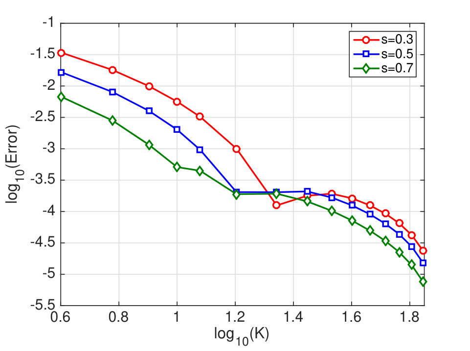
To test the accuracy of the proposed method, we add an external source term $f(\bm{x},t)$ so that the exact solution is $\psi(\bm{x},t)={\rm e}^{-|\bm{x}|^{2}-t}$ . In Figure 3.3 (a), we plot the maximum errors versus $\Delta t$ at $t=1$ , and the second-order convergence is observed. Here we take $\gamma=1$ , $N=10,$ $K=50$ and different $s,\mu$ . We choose the time stepping size to be small so that the error is dominated by the spatial error. In Figure 3.3 (b), we plot maximum errors in the semi-log scale versus various $K$ , for which we take $N=10$ , $\gamma=1$ and different $s,\mu$ . We observe that the spatial errors decay exponentially as $K$ increases.

(a) Temporal errors

(b) Spatial errors

Figure 3.3. (a): The temporal errors for Crank-Nicolson scheme at

t=1

with different

s,\mu

; (b): The spatial errors of GHF-spectral-Galerkin method at

t=1

with different

s,\mu

Next, we investigate the dynamics of beam propagations as in [42] (where the case $\mu=1$ was considered). We take the following incident Gaussian beam as the initial condition:

\psi(\bm{x},0)=\psi_{0}(\bm{x})={\rm e}^{-\sigma|\bm{x}|^{2}-{\rm i}C|\bm{x}|},

(3.30)

where the constants $\sigma$ and $C$ are the beam width and the linear chirp coefficient, respectively. In the test, we take $\sigma=C=1$ . In Figure 3.4, we depict the profiles of the real part of the numerical solutions for various $s,\mu$ at $t=2$ . Figure 3.4 (a) shows the solution profile of the usual case with a harmonic potential: $-\Delta+|\bm{x}|^{2}$ for comparison. We observe from the other profiles that the solutions have different peak intensities and singular behaviours, from which we find the smaller the value of $\mu,$ and the stronger the singularity. In fact, some similar observations was made in [42] for the case with $\mu=1.$

4. Müntz-type GHFs with applications to Schrödinger eigenvalue problems

In this section, we introduce the second family of generalised Hermite functions for efficient and spectrally accurate solutions of the Schrödinger eigenvalue problem:

\begin{cases}\big[\!-\frac{1}{2}\Delta+V(\bm{x})\big]u(\bm{x})=\lambda u(\bm{x})\quad&\text{in}\;\;\mathbb{R}^{d},\\[6.0pt] u(\bm{x})\to 0\quad&\text{as}\;\;|\bm{x}|\rightarrow\infty,\end{cases}

(4.1)

where the potential function $V(\bm{x})=Z|\bm{x}|^{2\alpha}$ with $\alpha,Z$ being given constants. It is known that (i) if $\alpha>-1$ , all eigenvalues of (4.1) are distinct; (ii) if $\alpha=-1$ or $Z=0$ , the spectrum of the Schrödinger operator $-\frac{1}{2}\Delta+\frac{Z}{|\bm{x}|^{2}}$ is a continuous one (cf. [13]).

The variational form of (4.1) is to find $\lambda\in\mathbb{R}$ and $u\in H^{1}(\mathbb{R}^{d})\setminus\{0\}$ such that

\mathcal{B}(u,v):=\frac{1}{2}(\nabla u,\nabla v)_{\mathbb{R}^{d}}+Z(|\bm{x}|^{2\alpha}u,v)_{\mathbb{R}^{d}}=\lambda(u,v)_{\mathbb{R}^{d}},\quad\forall\,v\in H^{1}(\mathbb{R}^{d}).

(4.2)

As shown in Theorem 2.2, the Hermite functions $\{\widehat{H}_{k,\ell}^{0,n}(\bm{x})\}$ are the eigenfunctions of the Schrödinger operator: $-\Delta+|\bm{x}|^{2}.$ Here, we intend to explore similar properties for the more general operator by introducing the Müntz-type Hermite functions, and construct efficient and spectrally accurate spectral approximation to (4.2).

4.1. Müntz-type generalised Hermite functions

To solve (4.2) accurately and efficiently, we introduce the following M-GHFs that are orthogonal in the sense of (4.5) below.

Definition 4.1.

For $\theta>0,(\ell,n)\in\Upsilon_{\infty}^{d}$ and $k\in\mathbb{N}_{0},$ the Müntz-type GHFs are defined by

\widehat{\mathcal{H}}^{\theta,n}_{k,\ell}(\bm{x})=c^{\theta,d}_{k,n}\,L^{(\beta_{n})}_{k}(|\bm{x}|^{2\theta})\mathrm{e}^{-\frac{|\bm{x}|^{2\theta}}{2}}Y^{n}_{\ell}(\bm{x}),\quad\bm{x}\in\mathbb{R}^{d},

(4.3)

where

c^{\theta,d}_{k,n}=\sqrt{\frac{2\,k!}{\Gamma(k+\beta_{n}+1)}},\quad\beta_{n}=\beta^{\theta,d}_{n}=\frac{n+d/2-1}{\theta}.

It is seen from (2.13) and (4.3) that if $\theta=1,$ it reduces the GHFs $\widehat{H}^{0,n}_{k,\ell}(\bm{x})$ , i.e., $\widehat{\mathcal{H}}^{1,n}_{k,\ell}(\bm{x})=\widehat{H}^{0,n}_{k,\ell}(\bm{x})$ . The so-defined Müntz-type GHFs enjoy the following remarkable properties, which are key to the success of the spectral algorithm for (4.2).

Theorem 4.1.

For $\theta>\max(1-d/2,0)$ , $(\ell,n),(\iota,m)\in\Upsilon^{d}_{\infty}$ and $k,j\in\mathbb{N}_{0}$ , we have

\big[\!-\Delta+\theta^{2}|\bm{x}|^{4\theta-2}\big]\widehat{\mathcal{H}}^{\theta,n}_{k,\ell}(\bm{x})=2\theta^{2}(\beta_{n}+2k+1)\,|\bm{x}|^{2\theta-2}\widehat{\mathcal{H}}^{\theta,n}_{k,\ell}(\bm{x}),

(4.4)

and the orthogonality

\displaystyle\begin{split}\big(\nabla\,\widehat{\mathcal{H}}^{\theta,n}_{k,\ell},\nabla\,\widehat{\mathcal{H}}^{\theta,m}_{j,\iota}\big)_{\mathbb{R}^{d}}+\theta^{2}\big(|\bm{x}|^{4\theta-2}\widehat{\mathcal{H}}^{\theta,n}_{k,\ell},\widehat{\mathcal{H}}^{\theta,m}_{j,\iota}\big)_{\mathbb{R}^{d}}=2\,\theta\,\big(\beta_{n}+2k+1\big)\delta_{jk}\delta_{mn}\delta_{\ell\iota}.\end{split}

(4.5)

Proof.

We can derive from (2.6), (2.10), (2.24), (4.3) and the change of variable $\rho=r^{\theta}$ that

		$\displaystyle\big[-\Delta+\theta^{2}r^{4\theta-2}\big]\widehat{\mathcal{H}}^{\theta,n}_{k,\ell}(\bm{x})$
		$\displaystyle=c^{\theta,d}_{k,n}\Big(-\frac{1}{r^{d-1}}\partial_{r}r^{d-1}\partial_{r}-\frac{1}{r^{2}}\Delta_{\mathbb{S}^{d-1}}+\theta^{2}r^{4\theta-2}\Big)\,[r^{n}\,L^{(\beta_{n})}_{k}(r^{2\theta})\mathrm{e}^{-\frac{r^{2\theta}}{2}}Y^{n}_{\ell}(\hat{\bm{x}})]$
		$\displaystyle=c^{\theta,d}_{k,n}\Big(-\frac{1}{r^{d-1}}\partial_{r}r^{d-1}\partial_{r}+\frac{n(n+d-2)}{r^{2}}+\theta^{2}r^{4\theta-2}\Big)\,[r^{n}\,L^{(\beta_{n})}_{k}(r^{2\theta})\mathrm{e}^{-\frac{r^{2\theta}}{2}}Y^{n}_{\ell}(\hat{\bm{x}})]$
		$\displaystyle=\theta^{2}\rho^{2-\frac{2}{\theta}}\Big(-\frac{1}{\rho^{\frac{d+2\theta-2}{\theta}-1}}\partial_{\rho}\rho^{\frac{d+2\theta-2}{\theta}-1}\partial_{\rho}+\frac{\frac{n}{\theta}(\frac{n}{\theta}+\frac{d+2\theta-2}{\theta}-2)}{\rho^{2}}+\rho^{2}\Big)\,[\rho^{\frac{n}{\theta}}\,L^{(\beta_{n})}_{k}(\rho^{2})\mathrm{e}^{-\frac{\rho^{2}}{2}}Y^{n}_{\ell}(\hat{\bm{x}})]$
		$\displaystyle=\theta^{2}\rho^{2-\frac{2}{\theta}}\Big(4k+\frac{2n}{\theta}+\frac{d+2\theta-2}{\theta}\Big)\,[\rho^{\frac{n}{\theta}}\,L^{(\beta_{n})}_{k}(\rho^{2})\mathrm{e}^{-\frac{\rho^{2}}{2}}Y^{n}_{\ell}(\hat{\bm{x}})]$
		$\displaystyle=2\theta^{2}\big(\beta_{n}+2k+1\big)r^{2\theta-2}[r^{n}\,L^{(\beta_{n})}_{k}(r^{2\theta})\mathrm{e}^{-\frac{r^{2\theta}}{2}}Y^{n}_{\ell}(\hat{\bm{x}})]$
		$\displaystyle=2\theta^{2}\big(\beta_{n}+2k+1\big)\|\bm{x}\|^{2\theta-2}\widehat{\mathcal{H}}^{\theta,n}_{k,\ell}(\bm{x}),$

where we used the identity derived from [21, Lemma 2.1] with $\alpha=\frac{n+d/2-1}{\theta}$ and $\beta=\alpha+\frac{1-d/2}{\theta}$ :

\begin{split}\Big[\partial_{\rho}^{2}+\frac{\frac{d+2\theta-2}{\theta}-1}{\rho}\partial_{\rho}-\frac{\frac{n}{\theta}(\frac{n}{\theta}+\frac{d+2\theta-2}{\theta}-2)}{\rho^{2}}-\rho^{2}+4k+\frac{2n}{\theta}+\frac{d+2\theta-2}{\theta}\Big]\big[\rho^{\frac{n}{\theta}}L_{k}^{(\beta_{n})}(\rho^{2})\,\mathrm{e}^{-\frac{\rho^{2}}{2}}\big]=0.\end{split}

Next, we prove the orthogonality (4.5). By virtue of (4.4), we have from (4.3) and the change of variable $\rho=r^{2\theta}$ that

	$\displaystyle\big(\nabla\,\widehat{\mathcal{H}}^{\theta,n}_{k,\ell},$	$\displaystyle\nabla\,\widehat{\mathcal{H}}^{\theta,m}_{j,\iota}\big)_{\mathbb{R}^{d}}+\theta^{2}\big(\|\bm{x}\|^{4\theta-2}\,\widehat{\mathcal{H}}^{\theta,n}_{k,\ell},\widehat{\mathcal{H}}^{\theta,m}_{j,\iota}\big)_{\mathbb{R}^{d}}$
		$\displaystyle=2\theta^{2}(\beta_{n}+2k+1)(c^{\theta,d}_{k,n})^{2}\delta_{mn}\delta_{\ell\iota}\!\int_{0}^{\infty}\!\!r^{2\theta+2n+d-3}L^{(\beta_{n})}_{k}(r^{2\theta})L^{(\beta_{n})}_{j}(r^{2\theta})\mathrm{e}^{-r^{2\theta}}\mathrm{d}r$
		$\displaystyle=\theta(\beta_{n}+2k+1)(c^{\theta,d}_{k,n})^{2}\delta_{mn}\delta_{\ell\iota}\int_{0}^{\infty}\rho^{\beta_{n}}L^{(\beta_{n})}_{k}(\rho)L^{(\beta_{n})}_{j}(\rho)\mathrm{e}^{-\rho}\mathrm{d}\rho$
		$\displaystyle=2\,\theta(\beta_{n}+2k+1)\,\delta_{mn}\delta_{jk}\delta_{\ell\iota}.$

This completes the proof. ∎

As a special case of (4.4) (i.e., $\theta=\frac{1}{2}$ ), we can find the explicit representation of the eigen-pairs of the Schrödinger operator with Coulomb potential: $-\frac{1}{2}\Delta-\frac{|Z|}{|\bm{x}|}$ in $d$ dimension, where $Z$ is a nonzero constant.

Corollary 4.1.

For any $k\in\mathbb{N}_{0},\,(\ell,n)\in\Upsilon_{\infty}^{d}$ and $Z\neq 0$ , we have

\Big[-\frac{1}{2}\Delta-\frac{|Z|}{|\bm{x}|}\Big]\widehat{\mathcal{H}}^{\frac{1}{2},n}_{k,\ell}\Big(\frac{4|Z|\,\bm{x}}{2n+2k+d-1}\Big)=-\frac{2Z^{2}}{(2n+2k+d-1)^{2}}\widehat{\mathcal{H}}^{\frac{1}{2},n}_{k,\ell}\Big(\frac{4|Z|\,\bm{x}}{2n+2k+d-1}\Big).

(4.6)

Proof.

Taking $\theta=\frac{1}{2}$ in (4.4) and rearranging the terms, leads to

\Big[\!-\Delta-\frac{\beta_{n}+2k+1}{2|\bm{x}|}\Big]\widehat{\mathcal{H}}^{\frac{1}{2},n}_{k,\ell}(\bm{x})=-\frac{1}{4}\widehat{\mathcal{H}}^{\frac{1}{2},n}_{k,\ell}(\bm{x}).

With a rescaling in $r$ direction

\bm{x}\to\frac{4|Z|\,\bm{x}}{\beta_{n}+2k+1}=\frac{4|Z|\,\bm{x}}{2n+2k+d-1},

we can obtain (4.6) immediately. ∎

The identity in Corollary 4.1 implies that the spectra of the Schrödinger operator with Coulomb potential are given by

\big\{\lambda_{i},u^{n}_{i,\ell}\big\}:=\bigg\{-\frac{2Z^{2}}{(2i+d-3)^{2}},\ \widehat{\mathcal{H}}^{\frac{1}{2},n}_{i-n-1,\ell}\Big(\frac{4|Z|\,\bm{x}}{2i+d-3}\Big)\bigg\},\quad(\ell,n)\in\Upsilon_{i-1}^{d},\ i\in\mathbb{N},

(4.7)

and the multiplicity of each $\lambda_{i}$ is

\displaystyle m_{i}^{d}:=a_{0}^{d}+a_{1}^{d}+\dots+a_{i-1}^{d}=\frac{(i-1)_{d-1}+(i)_{d-1}}{(d-1)!},\quad d\geq 2,

where we recall that $a_{i}^{d}$ (defined in (2.3)) is the cardinality of $\Upsilon_{i}^{d}\setminus\Upsilon_{i-1}^{d}$ (defined in (2.9)).

Remark 4.1.

The spectrum of the Schrödinger operator with Coulomb potential is of much interest in quantum mechanics and mathematical physics. For example, one can find the spectrum expressions in e.g., [26, P. 132] and [14, Thm. 10.10] for $d=3$ with a different derivation, and the recent work [25] for the asymptotic study of the eigenfunctions. ∎

Although the orthogonality (4.5) does not imply the orthogonality of each individual term, the stiffness and mass matrices are sparse with finite bandwidth.

Theorem 4.2.

For $\theta>\max(1-d/2,0)$ , $(\ell,n),(\iota,m)\in\Upsilon^{d}_{\infty}$ and $k,j\in\mathbb{N}_{0}$ , we have

\displaystyle\big(\nabla\widehat{\mathcal{H}}^{\theta,n}_{k,\ell},\nabla\widehat{\mathcal{H}}^{\theta,m}_{j,\iota}\big)_{\mathbb{R}^{d}}=\theta\,\delta_{mn}\delta_{\ell\iota}\times\begin{cases}\beta_{n}+2k+1,&j=k,\\ \sqrt{(k+1)\big(\beta_{n}+k+1\big)},&j=k+1,\\ \sqrt{(j+1)\big(\beta_{n}+j+1\big)},&k=j+1,\\ 0,&\text{otherwise},\end{cases}

(4.8)

and for $n+d/2+\alpha>0$ ,

\displaystyle\begin{split}&\big(|\bm{x}|^{2\alpha}\widehat{\mathcal{H}}^{\theta,n}_{k,\ell},\widehat{\mathcal{H}}^{\theta,m}_{j,\iota}\big)_{\mathbb{R}^{d}}=\frac{1}{2\theta}\,c^{\theta,d}_{k,n}\,c^{\theta,d}_{j,n}\,\delta_{mn}\,\delta_{\ell\iota}\\ &\qquad\qquad\times\sum_{p=0}^{\min(k,j)}\frac{\Gamma(k-p+1-\frac{1+\alpha}{\theta})\Gamma(j-p+1-\frac{1+\alpha}{\theta})\Gamma(p+\beta_{n}+\frac{1+\alpha}{\theta})}{\Gamma^{2}(1-\frac{1+\alpha}{\theta})\,(k-p)!\,(j-p)!\,p!}.\end{split}

(4.9)

Proof.

In view of the definition (4.3), we derive from (2.8), (2.11), (2.23) and the change of variable $\rho=r^{2\theta}$ , we derive

\begin{split}\big(|\bm{x}|^{2\alpha}&\widehat{\mathcal{H}}^{\theta,n}_{k,\ell},\widehat{\mathcal{H}}^{\theta,m}_{j,\iota}\big)_{\mathbb{R}^{d}}=c^{\theta,d}_{k,n}c^{\theta,d}_{j,n}\delta_{mn}\delta_{\ell\iota}\int_{0}^{\infty}r^{2n+d-1+2\alpha}L^{(\beta_{n})}_{k}(r^{2\theta})L^{(\beta_{n})}_{j}(r^{2\theta})\,\mathrm{e}^{-r^{2\theta}}\mathrm{d}r\\ &=\frac{1}{2\theta}c^{\theta,d}_{k,n}c^{\theta,d}_{j,n}\delta_{mn}\delta_{\ell\iota}\int_{0}^{\infty}\rho^{\frac{n+d/2-1}{\theta}+\frac{\alpha+1-\theta}{\theta}}L^{(\beta_{n})}_{k}(\rho)L^{(\beta_{n})}_{j}(\rho)\,\mathrm{e}^{-\rho}\mathrm{d}\rho\\ &=\frac{1}{2\theta}c^{\theta,d}_{k,n}c^{\theta,d}_{j,n}\delta_{mn}\delta_{\ell\iota}\sum_{p=0}^{k}\sum_{q=0}^{j}\frac{\Gamma(k-p+\frac{\theta-1-\alpha}{\theta})}{\Gamma(\frac{\theta-1-\alpha}{\theta})(k-p)!}\frac{\Gamma(j-q+\frac{\theta-1-\alpha}{\theta})}{\Gamma(\frac{\theta-1-\alpha}{\theta})(j-q)!}\\ &\quad\quad\times\int_{0}^{\infty}\rho^{\frac{n+d/2+\alpha-\theta}{\theta}}L^{(\frac{n+d/2+\alpha-\theta}{\theta})}_{p}(\rho)L^{(\frac{n+d/2+\alpha-\theta}{\theta})}_{q}(\rho)\,\mathrm{e}^{-\rho}\mathrm{d}\rho\\ &=\frac{c^{\theta,d}_{k,n}\,c^{\theta,d}_{j,n}}{2\theta}\,\delta_{mn}\,\delta_{\ell\iota}\sum_{p=0}^{\min(k,j)}\frac{\Gamma(k-p+\frac{\theta-1-\alpha}{\theta})\Gamma(j-p+\frac{\theta-1-\alpha}{\theta})\Gamma(p+\frac{n+d/2+\alpha}{\theta})}{\Gamma^{2}(\frac{\theta-1-\alpha}{\theta})\,(k-p)!\,(j-p)!\,p!},\end{split}

(4.10)

which gives (4.9). In particular, if $\alpha=2\theta-1$ , we derive from (4.10) that

\begin{split}\big(|\bm{x}|^{4\theta-2}\widehat{\mathcal{H}}^{\theta,n}_{k,\ell},\widehat{\mathcal{H}}^{\theta,m}_{j,\iota}\big)_{\mathbb{R}^{d}}&=\frac{1}{2\theta}c^{\theta,d}_{k,n}c^{\theta,d}_{j,n}\delta_{mn}\delta_{\ell\iota}\int_{0}^{\infty}\rho^{\beta_{n}+1}L^{(\beta_{n})}_{k}(\rho)L^{(\beta_{n})}_{j}(\rho)\,\mathrm{e}^{-\rho}\mathrm{d}\rho\\[4.0pt] &\,=\frac{1}{\theta}\,\delta_{mn}\delta_{\ell\iota}\times\begin{cases}\beta_{n}+2k+1,&j=k,\\ -\sqrt{(k+1)\big(\beta_{n}+k+1\big)},&j=k+1,\\ -\sqrt{(j+1)\big(\beta_{n}+j+1\big)},&k=j+1,\\ 0,&\text{otherwise}.\end{cases}\end{split}

(4.11)

Then (4.8) is a direct consequence of (4.5) and (4.11). Note that (4.11) can be also obtained from (4.10) with the understanding $\Gamma(z)=0$ if $z$ is negative integer. ∎

4.2. Schrödinger eigenvalue problem with a Coulomb potential

In what follows, we implement the Hermite spectral method for the three-dimensional Schrödinger eigenvalue problem (4.1) with a Coulomb potential $V(\bm{x})=\frac{Z}{|\bm{x}|}$ with $Z<0$ for the hydrogen atom [34], that is,

\displaystyle\Big(-\frac{1}{2}\Delta+\frac{Z}{|\bm{x}|}\Big)u(\bm{x})=\lambda u(\bm{x}),\quad\bm{x}\in\mathbb{R}^{3}.

(4.12)

Numerical solution of (4.12) poses at least two challenges (i) nonpositive definiteness of the variational form and (ii) the singularity of the Coulomb potential. To overcome these, we shall propose an efficient and accurate spectral method by using the Müntz-type GHFs with a suitable parameter $\theta=\frac{1}{2}$ , in light of the Coulomb potential.

Define the approximation space

\displaystyle\mathcal{W}_{\!N,K}=\text{span}\big\{\widehat{{\mathcal{H}}}_{k,\ell}^{\frac{1}{2},n}(\kappa\bm{x}):\;0\leq n\leq N,\;1\leq\ell\leq 2n+1,~0\leq k\leq K,\;k,\ell,n\in{\mathbb{N}}_{0}\big\},

where a scaling factor $\kappa>0$ is used to enhance the performance of the spectral approximation as in usual Hermite spectral methods in one dimension (see, e.g., [38, 31]). The spectral approximation scheme for (4.2) is to find $\lambda_{\!N,K}\in\mathbb{R}$ and $u_{\!N,K}\in\mathcal{W}_{\!N,K}\setminus\{0\}$ such that

\mathcal{B}(u_{\!N,K},v_{\!N,K})=\lambda_{\!N,K}(u_{\!N,K},v_{\!N,K})_{\mathbb{R}^{3}},\quad\forall\,v_{\!N,K}\in\mathcal{W}_{\!N,K}.

(4.13)

In real implementation, we write

\displaystyle u_{\!N,K}(\bm{x})=\sum_{n=0}^{N}\sum_{\ell=1}^{2n+1}\sum_{k=0}^{K}\hat{u}_{k,\ell}^{n}\,\widehat{{\mathcal{H}}}_{k,\ell}^{\frac{1}{2},n}(\kappa\bm{x}),

and denote

\begin{split}\hat{\bm{u}}^{n}_{\ell}=\big(\hat{u}^{n}_{0,\ell},\hat{u}^{n}_{1,\ell},\dots,\hat{u}^{n}_{K,\ell}\big)^{t},\quad\bm{u}=\big(\hat{\bm{u}}_{1}^{0},\hat{\bm{u}}_{1}^{1},\hat{\bm{u}}_{2}^{1},\hat{\bm{u}}_{3}^{1},\cdots,\hat{\bm{u}}_{1}^{N},\hat{\bm{u}}_{2}^{N},\cdots,\hat{\bm{u}}_{2N+1}^{N}\big)^{t}.\end{split}

(4.14)

With this ordering, we denote the stiffness and the mass matrices by $\bm{S}$ and $\bm{M},$ respectively, with the entries given by

	$\displaystyle\mathcal{B}(\widehat{\mathcal{H}}^{\frac{1}{2},n}_{k,\ell}(\kappa\cdot),\widehat{\mathcal{H}}^{\frac{1}{2},m}_{j,\iota}(\kappa\cdot))=$	$\displaystyle\,\frac{1}{2\kappa}\Big[(\nabla\,\widehat{\mathcal{H}}^{\frac{1}{2},n}_{k,\ell},\nabla\widehat{\mathcal{H}}^{\frac{1}{2},m}_{j,\iota})_{\mathbb{R}^{3}}+\frac{1}{4}(\widehat{\mathcal{H}}^{\frac{1}{2},n}_{k,\ell},\widehat{\mathcal{H}}^{\frac{1}{2},m}_{j,\iota})_{\mathbb{R}^{3}}\Big]$
		$\displaystyle\,+\frac{Z}{\kappa^{2}}\big(\|\bm{x}\|^{-1}\widehat{\mathcal{H}}^{\frac{1}{2},n}_{k,\ell},\widehat{\mathcal{H}}^{\frac{1}{2},m}_{j,\iota}\big)_{\mathbb{R}^{3}}-\frac{1}{8\kappa}\big(\widehat{\mathcal{H}}^{\frac{1}{2},n}_{k,\ell},\widehat{\mathcal{H}}^{\frac{1}{2},m}_{j,\iota}\big)_{\mathbb{R}^{3}},$
	$\displaystyle\big(\widehat{\mathcal{H}}^{\frac{1}{2},n}_{k,\ell}(\kappa\cdot),\widehat{\mathcal{H}}^{\frac{1}{2},m}_{j,\iota}(\kappa\cdot)\big)_{\mathbb{R}^{3}}=$	$\displaystyle\,\frac{1}{\kappa^{3}}\big(\widehat{\mathcal{H}}^{\frac{1}{2},n}_{k,\ell},\widehat{\mathcal{H}}^{\frac{1}{2},m}_{j,\iota}\big)_{\mathbb{R}^{3}}.$

Owing to (4.5) and (4.11) with $\theta=\frac{1}{2}$ , both the stiffness matrix $\bm{S}$ and the mass matrix $\bm{M}$ are tridiagonal.

Consequently, the scheme (4.13) has an equivalent form in the following algebraic eigen-system:

\bm{S}\bm{u}=\lambda_{\!N}\bm{M}\bm{u}.

(4.15)

Interestingly, the matrix $\bm{S}+\frac{\kappa^{2}}{8}\bm{M}$ is diagonal, so we can rewrite (4.15) as

\displaystyle\Big(\bm{S}+\frac{\kappa^{2}}{8}\bm{M}\Big)\bm{u}=\Big(\lambda_{N}+\frac{\kappa^{2}}{8}\Big)\bm{M}\bm{u},

which leads a more efficient implementation.

(a)

N=16

and

\kappa=4

(b)

N=16

and

\kappa=7/4

Figure 4.1. The errors of the smallest

4

eigenvalues without counting multiplicities versus

K

for solving (4.12) with

Z=-1

In Figure 4.1, we plot the errors between the first $30$ (counted by multiplicity) smallest numerical eigenvalues and exact eigenvalues in (4.7) versus $K$ for fixed $N=16$ and two different scaling factors (so that the error of the truncation in angular directions is negligible). Observe that the errors decay exponentially in terms of the cut-off number in the radial direction, along which the eigenfunctions are singular. We also see that the scaling parameter affects the convergence rate as the usual Hermite method (cf. [38]).

4.3. Schrödinger eigenvalue problem with a fractional power potential

Note that for any given rational number $\frac{q}{p}>-2$ with $p\in\mathbb{N}$ and $q\in\mathbb{Z}$ , we can always rewrite it as

\frac{q}{p}=\frac{2\nu-2\mu}{\mu+1}\quad{\rm with}\;\;\;\mu=2p-1\in\mathbb{N},\;\;\nu=2p+q-1\in\mathbb{N}_{0}.

(4.16)

In the sequel, we consider the following Schrödinger equation with a fractional power potential as follows

\displaystyle-\frac{1}{2}\Delta u(\bm{x})+Z|\bm{x}|^{\frac{2\nu-2\mu}{\mu+1}}\,u(\bm{x})=\lambda u(\bm{x}),\qquad\bm{x}\in\mathbb{R}^{d},

(4.17)

where $\mu,\nu\in\mathbb{N}_{0}.$ Hereafter, we choose the Müntz-type GHF approximation with $\theta=\frac{1}{\mu+1},$ to account for both the accuracy and efficiency. Accordingly, we define the approximation space

\displaystyle\mathcal{W}_{\!N,K}^{d,\frac{1}{\mu+1}}=\text{span}\big\{\widehat{{\mathcal{H}}}_{k,\ell}^{\frac{1}{\mu+1},n}(\kappa\bm{x}):\;0\leq n\leq N,\;1\leq\ell\leq a_{n}^{d},~0\leq k\leq K,\;k,\ell,n\in{\mathbb{N}}_{0}\big\},\quad d\geq 2,

and for $d=1$ , we can always assume $\mu$ is odd and then define the approximation space as

\displaystyle\mathcal{W}_{\!N,K}^{1,\frac{1}{\mu+1}}=\text{span}\big\{\widehat{{\mathcal{H}}}_{k,1}^{\frac{1}{\mu+1},n}(\kappa\bm{x}):\;\frac{\mu+1}{2}\delta_{n,0}\leq k\leq K,\ n=0,1\big\},

where $\{\widehat{{\mathcal{H}}}_{k,1}^{\frac{1}{\mu+1},n}\}$ are understood as the Müntz-type GHFs defined through generalized Laguerre polynomials $L^{(\beta_{0})}_{k}$ with the negative integer $\beta_{0}=-\frac{\mu+1}{2}$ (cf. [19]). This turns out important to deal with the strong singularities at the origin to ensure $u(0)=0$ in one dimension.

The generalized Hermite spectral method for (4.2) is to find $\lambda_{\!N,K}\in\mathbb{R}$ and $u_{\!N,K}\in\mathcal{W}^{d,\frac{1}{\mu+1}}_{\!N,K}\setminus\{0\}$ such that

\mathcal{B}(u_{\!N,K},v_{\!N,K})=\lambda_{\!N,K}(u_{\!N,K},v_{\!N,K})_{\mathbb{R}^{d}},\quad\forall\,v_{\!N,K}\in\mathcal{W}^{d,\frac{1}{\mu+1}}_{\!N,K}.

(4.18)

In the implementation, we write

\displaystyle u_{\!N,K}(\bm{x})=\sum_{n=0}^{N}\sum_{\ell=1}^{a_{n}^{d}}\sum_{k=0}^{K}\hat{u}_{k,\ell}^{n}\,\widehat{{\mathcal{H}}}_{k,\ell}^{\frac{1}{\mu+1},n}(\kappa\bm{x}),

and denote

\begin{split}\hat{\bm{u}}^{n}_{\ell}=\big(\hat{u}^{n}_{0,\ell},\hat{u}^{n}_{1,\ell},\dots,\hat{u}^{n}_{K,\ell}\big)^{t},\quad\bm{u}=\big(\hat{\bm{u}}_{1}^{0},\hat{\bm{u}}_{2}^{0},\cdots,\hat{\bm{u}}_{a_{0}^{d}}^{0},\hat{\bm{u}}_{1}^{1},\hat{\bm{u}}_{2}^{1},\cdots,\hat{\bm{u}}_{a_{1}^{d}}^{1},\cdots,\hat{\bm{u}}_{1}^{N},\hat{\bm{u}}_{2}^{N},\cdots,\hat{\bm{u}}_{a_{N}^{d}}^{N}\big)^{t}.\end{split}

(4.19)

The corresponding algebraic eigen-system of (4.18) is

\bm{S}\bm{u}=\lambda_{\!N}\bm{M}\bm{u}.

(4.20)

In view of orthogonality (4.8) and (4.9), we find that for any $q\in\mathbb{N}_{0}$ ,

		$\displaystyle\big(\|\bm{x}\|^{\frac{2q-2\mu}{\mu+1}}\widehat{\mathcal{H}}^{\frac{1}{\mu+1},n}_{k,\ell}(\kappa\cdot),\widehat{\mathcal{H}}^{\frac{1}{\mu+1},m}_{j,\iota}(\kappa\cdot)\big)_{\mathbb{R}^{d}}=\kappa^{-d}\big(\widehat{\mathcal{H}}^{\frac{1}{\mu+1},n}_{k,\ell},\widehat{\mathcal{H}}^{\frac{1}{\mu+1},m}_{j,\iota}\big)_{\mathbb{R}^{d}}$
		$\displaystyle=\frac{\mu+1}{2}\kappa^{-d}\,c^{\frac{1}{\mu+1},d}_{k,n}\,c^{\frac{1}{\mu+1},d}_{j,n}\,\delta_{mn}\,\delta_{\ell\iota}\sum_{p=\max(j-q,k-q,0)}^{\min(k,j)}\frac{\Gamma(k-p-q)\Gamma(j-p-q)\Gamma(p+\beta_{n}+q+1)}{\Gamma^{2}(-q)\,(k-p)!\,(j-p)!\,p!}$
		$\displaystyle=\frac{\mu+1}{2}\kappa^{-d}\,c^{\frac{1}{\mu+1},d}_{k,n}\,c^{\frac{1}{\mu+1},d}_{j,n}\,\delta_{mn}\,\delta_{\ell\iota}\sum_{p=\max(j-q,k-q,0)}^{\min(k,j)}\frac{(-q)_{k-p}(-q)_{j-p}\Gamma(p+\beta_{n}+q+1)}{(k-p)!\,(j-p)!\,p!}.$

Furthermore, one has

	$\displaystyle\mathcal{B}(\widehat{\mathcal{H}}^{\frac{1}{\mu+1},n}_{k,\ell}(\kappa\cdot),\widehat{\mathcal{H}}^{\frac{1}{\mu+1},m}_{j,\iota}(\kappa\cdot))$	$\displaystyle=\frac{1}{2}\,\kappa^{2-d}(\nabla\,\widehat{\mathcal{H}}^{\frac{1}{\mu+1},n}_{k,\ell},\nabla\widehat{\mathcal{H}}^{\frac{1}{\mu+1},m}_{j,\iota})_{\mathbb{R}^{d}}$
		$\displaystyle\quad+Z\,\kappa^{-\frac{2\nu-2\mu}{\mu+1}-d}(\|\bm{x}\|^{\frac{2\nu-2\mu}{\mu+1}}\widehat{\mathcal{H}}^{\frac{1}{\mu+1},n}_{k,\ell},\widehat{\mathcal{H}}^{\frac{1}{\mu+1},m}_{j,\iota})_{\mathbb{R}^{d}}.$

These indicate that the stiffness matrix $\bm{S}$ is a sparse banded matrix with a bandwidth $\max(\nu,1)$ , and the mass matrix $\bm{M}$ is also a sparse banded matrix with a bandwidth $\mu$ .

(a)

d=4

Z=1

\mu=3

\nu=5

and

\kappa=500

(b)

d=3

Z=1

\mu=1

\nu=2

and

\kappa=2

(c)

d=2

Z=3

\mu=1

\nu=4

and

\kappa=10

(d)

d=1

Z=-3

\mu=3

\nu=2

and

\kappa=70

Figure 4.2. The errors of the smallest

5

eigenvalues without counting multiplicities versus

K

for solving (4.17) with

N=10

In the numerical tests, we fix $N=10$ , choose different scaling factor $\kappa$ and test for different $Z$ , $\mu,\nu$ and dimensions. Numerical errors between the smallest eigenvalues without counting multiplicities and the reference eigenvalues (obtained by the scheme with large $N$ and $K$ ) are depicted in Figure 4.2. Exponential orders of convergence are clearly observed in all cases, which demonstrate the effectiveness of the new Hermite spectral method.

Acknowledgement: The first author would like to thank Beijing Computational Science Research Center for hosting his visit devoted to this collaborative work. The fourth author is grateful to Professor Jie Shen at Purdue University for valuable suggestion.

Appendix A The proof of Theorem 2.4

We first recall the orthogonality (cf. [9, (11.6)])

\displaystyle\int_{\mathbb{R}}H_{m}^{(\mu)}(x)H_{n}^{(\mu)}(x)|x|^{2\mu}\,\mathrm{e}^{-x^{2}}\,\mathrm{d}x=\gamma_{n}^{(\mu)}\delta_{mn},\quad\gamma_{n}^{(\mu)}=2^{2n}\,\Big[\frac{n}{2}\Big]!\,\Gamma\Big(\Big[\frac{n+1}{2}\Big]+\mu+\frac{1}{2}\Big).

(A.1)

According to [9, P. 42], we have

\partial_{x}H_{n}^{(\mu)}(x)=2nH_{n-1}^{(\mu)}(x)+2(n-1)\theta_{n}\,x^{-1}H_{n-2}^{(\mu)}(x),\quad n\geq 1,

(A.2)

where $\theta_{2k}=0$ and $\theta_{2k+1}=2\mu$ as in (2.43). In particular, for $\mu>-\frac{1}{2},$

\partial_{x}H^{(\mu)}_{2k}(x)=4kH^{(\mu)}_{2k-1}(x),\quad k\geq 1.

(A.3)

We first show the modified derivative (cf. (2.52)) formula: for $k\geq m,$

D_{x}^{m}H^{(\mu)}_{2k}(x)=d_{k}^{(m)}H^{(\mu+m-1)}_{2k-2m+1}(x),\quad D_{x}^{m}H^{(\mu)}_{2k+1}(x)=d_{k}^{(m)}H^{(\mu+m)}_{2k-2m+1}(x),\;\;\;d_{k}^{(m)}=\frac{4^{m}k!}{(k-m)!}.

(A.4)

For this purpose, we recall the recurrence relation (cf. [30, P. 609]):

2xH^{(\mu+1)}_{2k}(x)=H^{(\mu)}_{2k+1}(x),\quad k\geq 0,

(A.5)

which, together with (A.3), implies

D_{x}H^{(\mu)}_{2k+1}(x)=\partial_{x}\Big\{\frac{1}{2x}H^{(\mu)}_{2k+1}(x)\Big\}=\partial_{x}H^{(\mu+1)}_{2k}(x)=4kH^{(\mu+1)}_{2k-1}(x).

(A.6)

Thus, we obtain from (2.52) that

D_{x}^{2}H^{(\mu)}_{2k+1}(x)=4kD_{x}H^{(\mu+1)}_{2k-1}(x)=4^{2}k(k-1)H^{(\mu+2)}_{2k-3}(x).

(A.7)

Using this relation repeatedly yields the second identity in (A.4). We now consider the first identity. For $m=1,$ it coincides with (A.3), so by (A.6),

D_{x}^{2}H^{(\mu)}_{2k}(x)=4kD_{x}H^{(\mu)}_{2k-1}(x)=4k\partial_{x}\Big\{\frac{1}{2x}H^{(\mu)}_{2k-1}(x)\Big\}=4^{2}k(k-1)H^{(\mu+1)}_{2k-3}(x),

(A.8)

which leads to the first identity by taking higher modified derivatives and the second identity in (A.4).

For the orthogonal projection defined in (2.48), we can write

\Pi^{(\mu)}_{N}u(x)=\sum_{n=0}^{N}\tilde{u}_{n}H^{(\mu)}_{n}(x)=\sum_{k=0}^{[\frac{N}{2}]}\tilde{u}_{2k}H^{(\mu)}_{2k}(x)+\sum_{k=0}^{[\frac{N}{2}]}\tilde{u}_{2k+1}H^{(\mu)}_{2k+1}(x),

(A.9)

with

\tilde{u}_{n}=\frac{1}{\gamma^{(\mu)}_{n}}\int_{\mathbb{R}}u(x)H^{(\mu)}_{n}(x)\chi^{(\mu)}(x)\,\mathrm{d}x.

We only need to prove show the result with $m\geq 1$ , as $m=0$ is obvious. For simplicity, we first assume that $N$ is odd. It is clear that by (A.9),

\|\Pi^{(\mu)}_{N}u-u\|^{2}_{\chi^{(\mu)}}=\|\Pi^{(\mu)}_{N}u_{\rm e}-u_{\rm e}\|^{2}_{\chi^{(\mu)}}+\|\Pi^{(\mu)}_{N}u_{\rm o}-u_{\rm o}\|^{2}_{\chi^{(\mu)}},

(A.10)

where we decompose $u(x)$ into even and odd parts as $u_{\rm e}(x)$ and $u_{\rm o}(x)$ . We now deal with the first term. By (A.1) and (A.4), we have the orthogonality

\displaystyle\int_{\mathbb{R}}D_{x}^{m}H_{2k}^{(\mu)}(x)\,D_{x}^{m}H_{2l}^{(\mu)}(x)\chi^{(\mu+m-1)}(x)\,\mathrm{d}x=h_{2k,m}^{(\mu)}\,\delta_{k,l},

(A.11)

where for $k\geq m$ ,

\begin{split}h_{2k,m}^{(\mu)}=(d_{k}^{(m)})^{2}\gamma_{2k-2m+1}^{(\mu+m-1)}=\frac{2^{4k+2}\,\Gamma(k+\mu+\frac{1}{2})(k!)^{2}}{(k-m)!}.\end{split}

(A.12)

Thus, by the Parseval’s identity, we have

\|D_{x}^{m}u_{\rm e}\|_{\chi^{(\mu+m-1)}}^{2}=\sum_{k=m}^{\infty}h_{2k,m}^{(\mu)}|\tilde{u}_{2k}|^{2}.

In view of (A.11), we obtain from (A.12) that for $m\geq 1,$

\begin{split}\big\|\Pi_{N}^{(\mu)}u_{\rm e}-u_{\rm e}\big\|_{\chi^{(\mu)}}^{2}&=\sum_{k=\frac{N+1}{2}}^{\infty}\gamma_{2k}^{(\mu)}|\tilde{u}_{2k}|^{2}\leq\max_{k\geq\frac{N+1}{2}}\Big\{\frac{\gamma_{2k}^{(\mu)}}{h_{2k,m}^{(\mu)}}\Big\}\sum_{k=\frac{N+1}{2}}^{\infty}h_{2k,m}^{(\mu)}|\tilde{u}_{2k}|^{2}\\ &\leq\frac{\gamma_{N+1}^{(\mu)}}{h_{N+1,m}^{(\mu)}}\big\|D_{x}^{m}u_{\rm e}\big\|_{\chi^{(\mu+m-1)}}^{2}\leq\frac{(\frac{N+1}{2}-m)!}{2^{2}(\frac{N+1}{2})!}\big\|D_{x}^{m}u_{\rm e}\big\|_{\chi^{(\mu+m-1)}}^{2}.\end{split}

(A.13)

Similarly, by (A.4) and (A.1), we have the orthogonality

\displaystyle\int_{\mathbb{R}}D_{x}^{m}H_{2k+1}^{(\mu)}(x)\,D_{x}^{m}H_{2l+1}^{(\mu)}(x)\chi^{(\mu+m)}(x)\,\mathrm{d}x=h_{2k+1,m}^{(\mu)}\,\delta_{k,l},

(A.14)

where for $k\geq m$ ,

\begin{split}h_{2k+1,m}^{(\mu)}=(d_{k}^{(m)})^{2}\gamma_{2k-2m+1}^{(\mu+m)}=\frac{2^{4k+2}\,\Gamma(k+\mu+\frac{3}{2})(k!)^{2}}{(k-m)!}.\end{split}

Then, following the same lines as above, we can show

\begin{split}\big\|\Pi_{N}^{(\mu)}u_{\rm o}-u_{\rm o}\big\|_{\chi^{(\mu)}}^{2}&\leq\frac{\gamma_{N+2}^{(\mu)}}{h_{N+2,m}^{(\mu)}}\|D_{x}^{m}u_{\rm o}\|_{\chi^{(\mu+m)}}^{2}\leq\frac{(\frac{N+1}{2}-m)!}{(\frac{N+1}{2})!}\|D_{x}^{m}u_{\rm o}\|_{\chi^{(\mu+m)}}^{2}.\end{split}

(A.15)

Thus, a combination of (A.10), (A.13) and (A.15) leads to the estimate (2.53) with odd $N.$ For even $N,$ we can obtain the same estimate but with $N/2$ in place of $(N+1)/2$ in the upper bound.

Now, we turn to the proof of (2.54). If $ue^{\frac{x^{2}}{2}}\in{{\mathcal{B}}}_{\mu}^{m}(\mathbb{R}),$ we find from (2.49) that

\big\|u-\widehat{\Pi}^{(\mu)}_{N}u\big\|_{\omega^{(\mu)}}=\big\|u\mathrm{e}^{\frac{x^{2}}{2}}-{\Pi}^{(\mu)}_{N}(u\mathrm{e}^{\frac{x^{2}}{2}})\big\|_{\chi^{(\mu)}}.

(A.16)

Then the estimate (2.54) is a direct consequence of (2.53).

References

[1] M. S. Agranovich. Sobolev spaces, their generalizations and elliptic problems in smooth and Lipschitz domains. Springer Monographs in Mathematics. Springer, Cham, 2015.
[2] G. E. Andrews, R. Askey and R. Roy. Special functions. Cambridge, 1999.
[3] R. Askey. Orthogonal polynomials and special functions. Society for Industrial and Applied Mathematics, 1975.
[4] W. Bao, H. Li and J. Shen. A generalized Laguerre-Fourier-Hermite pseudospectral method for computing the dynamics of rotating Bose-Einstein condensates. SIAM J. Sci. Comput., 31(5): 3685-3711, 2009.
[5] W. Bao, X. Ruan, J. Shen and C. Sheng. Fundamental gaps of the fractional Schrödinger operator. Commun. Math. Sci., 17(2): 447-471, 2019.
[6] W. Bao, L. Chen, X. Jiang and Y. Ma. A Jacobi spectral method for computing eigenvalue gaps and their distribution statistics of the fractional Schrödinger operator. J. Comput. Phys., 421: 109733, 2020.
[7] D. Burnett. The distribution of molecular velocities and the mean motion in a non-uniform gas. Proc. London Math. Soc., 40(1): 382-435, 1936.
[8] Z. Cai, Y. Fan and Y. Wang. Burnett spectral method for the spatially homogeneous Boltzmann equation. Comput. & Fluids, 200: 104456, 2020.
[9] T. Chihara. Generalized Hermite polynomials. PhD Thesis, Purdue University, 1955.
[10] T. Chihara. An introduction to orthogonal polynomials. New York-London-Paris, 1978.
[11] F. Dai and Y. Xu. Approximation theory and harmonic analysis on spheres and balls. Springer-Verlag, 2013.
[12] E. Di Nezza, G. Palatucci and E. Valdinoci. Hitchhiker’s guide to the fractional Sobolev spaces. Bull. Sci. Math., 136(5): 521-573, 2012.
[13] Z. J. Duoandikoetxea. Fourier analysis, vol. 29, American Mathematical Society. 2001.
[14] T. Gerald, Mathematical methods in quantum mechanics with applications to Schrödinger operators. Second edition. Graduate Studies in Mathematics, 157. American Mathematical Society, Providence, RI, 2014.
[15] I. S. Gradshteyn and I. M. Ryzhik, Table of Integrals, Series, and Products, Elsevier/Academic Press, Amsterdam, eighth ed., 2015. Translated from the Russian, Translation edited and with a preface by Daniel Zwillinger and Victor Moll.
[16] D. Hou and C. Xu. A fractional spectral method with applications to some singular problems. Adv. Comput. Math., 43(5): 911-944, 2017.
[17] Z. Hu and Z. Cai. Burnett spectral method for high-speed rarefied gas flows. SIAM J. Sci. Comput., 42(5): 1193-1226, 2020.
[18] N. Laskin. Fractional quantum mechanics and Lévy path integrals. Physics Letters A, 268(4-6): 298-305, 2000.
[19] F. Liu, Z. Wang and H. Li. A fully diagonalized spectral method using generalized Laguerre functions on the half line. Adv. Comput. Math., 43(6): 1227-1259, 2017.
[20] C. Lubich. From quantum to classical molecular dynamics: reduced models and numerical analysis. European Mathematical Society, Zürich, 2008.
[21] S. Ma, H. Li and Z. Zhang. Novel spectral methods for Schrödinger equations with an inverse square potential on the whole space. Discrete Contin. Dyn. Syst. Ser. B , 24(4): 1589-1615, 2019.
[22] Z. Mao and J. Shen. Hermite spectral methods for fractional PDEs in unbounded domains. SIAM J. Sci. Comput., 39(5): A1928-A1950, 2017.
[23] M. Masjed-Jamei and W. Koepf. Two classes of special functions using Fourier transforms of generalized ultraspherical and generalized Hermite polynomials. Proc. Amer. Math. Soc., 140 (6): 2053-2063, 2012.
[24] Ch. H. Müntz. Über den Approximationssatz von Weierstrass, in H. A. Schwarz’s Festschrift, Berlin, pp. 303–312, 1914.
[25] V. I. Osherov and V. G. Ushakov. Analytical solutions of the Schrödinger equation for a hydrogen atom in a uniform electric field. Phys. Rev. A., 95: 023419, 2017.
[26] L. Pauling and E. B. Wilson. Introduction to quantum mechanics with applications to Chemistry. McGraw-Hill, 1935.
[27] L. P. Pitaevskii and S. Stringari. Bose-Einstein condensation. The Clarendon Press, Oxford University Press, Oxford, 2003.
[28] M. Rosenblum. Generalized Hermite polynomials and the Bose-like oscillator calculus. Nonselfadjoint operators and related topics. Oper. Theory Adv. Appl., 73: 369-396, 1994.
[29] M. Rösler. Generalized Hermite polynomials and the heat equation for Dunkl operators. Comm. Math. Phys., 192(3): 519-542, 1998.
[30] T. S. Shao, T. C. Chen, and R. M. Frank. Tables of zeros and Gaussian weights of certain associated Laguerre polynomials and the related generalized Hermite polynomials. Math. Comput., 18: 598-616, 1964.
[31] J. Shen, T. Tang and L.-L. Wang, Spectral methods: algorithms, analysis and applications. Springer, 2011.
[32] J. Shen and Y. Wang. Müntz-Galerkin methods and applications to mixed Dirichlet-Neumann boundary value problems. SIAM J. Sci. Comput., 38: A2357-A2381, 2016.
[33] C. Sheng, J. Shen, T. Tang, L.-L. Wang and H. Yuan. Fast Fourier-like mapped Chebyshev spectral-Galerkin methods for PDEs with integral fractional Laplacian in unbounded domains. SIAM J. Numer. Anal., 58(5): 2435-2464, 2020.
[34] E. Schrödinger. Quantisierung als Eigenwertproblem. Annalen der Physik. 384(4): 361–377, 1926.
[35] G. Strang and G. Fix. An analysis of the finite element method. Prentice-Hall Inc., Englewood Cliffs, N. J., prentice-Hall Series in Automatic Computation, 1973.
[36] O. Szász. Über die Approximation stetiger funktionen durch lineare aggregate von potenzen. Math. Ann., 77: 482-496, 1916.
[37] G. Szegö. Orthogonal polynomials. American Mathematical Society, Providence, 1939.
[38] T. Tang. The Hermite spectral method for Gaussian-type functions. SIAM J. Sci. Comput., 14(3): 594-606, 1993.
[39] T. Tang, H. Yuan and T. Zhou. Hermite spectral collocation methods for fractional PDEs in unbounded domains. Commun. Comput. Phys., 24(4): 1143-1168, 2018.
[40] A. Yurova. Generalized anisotropic Hermite functions and their applications. PhD Thesis, Technische Universität München, 2020.
[41] J. Zhang, H. Li, L.-L. Wang and Z. Zhang. Ball prolate spheroidal wave functions in arbitrary dimensions. Appl. Comput. Harmon. Anal., 48(2): 539-569, 2020.
[42] Y. Zhang, X. Liu, M. Belić, et. al.. Propagation dynamics of a light beam in a fractional Schrödinger equation. Phys. Rev. Lett., 115(18): 180403, 2015.

Abstract.

Key words and phrases:

2000 Mathematics Subject Classification

1. Introduction

2. Generalized Hermite polynomials/functions in multiple dimensions

2.1. Preliminaries

2.2. Generalized Hermite polynomials/functions in ℝd\mathbb{R}^{d}

Definition 2.1.

Remark 2.1.

Theorem 2.1.

Proof.

Proposition 2.1.

Proof.

Proposition 2.2.

Proof.

Remark 2.2.

Theorem 2.2.

Proof.

2.3. Adjoint generalized Hermite functions in ℝd\mathbb{R}^{d}

Definition 2.2.

Remark 2.3.

Theorem 2.3.

Proof.

Corollary 2.1.

Remark 2.4.

Remark 2.5.

2.4. Differences and connections with some existing generalisations

2.4.1. GHPs/GHFs in Szegö [37]

Theorem 2.4.

Remark 2.6.

2.4.2. 2D GHFs versus generalised Hermite bases for Bose-Einstein condensates in [4]

2.4.3. 3D GHPs versus Burnett polynomials [7]

3. GHF approximation of the IFL and the Schrödinger equation

3.1. GHF-spectral-Galerkin method for a fractional model problem

Remark 3.1.

3.1.1. Error analysis

Theorem 3.1.

Proof.

Theorem 3.2.

3.1.2. Numerical results

Example 1.

Example 2.

3.2. GHF-spectral-Galerkin method for fractional Schrödinger equations

4. Müntz-type GHFs with applications to Schrödinger eigenvalue problems

4.1. Müntz-type generalised Hermite functions

Definition 4.1.

Theorem 4.1.

Proof.

Corollary 4.1.

Proof.

Remark 4.1.

Theorem 4.2.

Proof.

4.2. Schrödinger eigenvalue problem with a Coulomb potential

4.3. Schrödinger eigenvalue problem with a fractional power potential

Appendix A The proof of Theorem 2.4

References

2.2. Generalized Hermite polynomials/functions in $\mathbb{R}^{d}$

2.3. Adjoint generalized Hermite functions in $\mathbb{R}^{d}$