Factorization of the Partial Covariance in Singly-Connected Path Diagrams
Abstract.
We extend path analysis by showing that, for a singly-connected path diagram, the partial covariance of two random variables factorizes over the nodes and edges in the path between the variables. This result allows us to determine the contribution of each node and edge to the partial covariance. It also allows us to show that Simpson’s paradox cannot occur in singly-connected path diagrams.
1. Introduction
To ease interpretation, linear structural equation models are typically represented as path diagrams: Nodes represent random variables, directed edges represent direct causal relationships, and bidirected edges represent confounding, i.e. correlation between error terms. Moreover, each directed edge is annotated with the corresponding coefficient in the linear structural equation model, a.k.a. path coefficient. Likewise, each bidirected edge is annotated with the corresponding error correlation. A path diagram also brings in computational benefits. For instance, the covariance of two random variables and can be determined from the path diagram. Specifically, can be expressed as the sum over the paths from to of the product of path coefficients and error covariances of the edges in the path (Wright 1921; Pearl 2009). Hence, the covariance factorizes over the edges and nodes in the paths. In this work, we develop a similar factorization for the partial covariance in singly-connected path diagrams, i.e. the underlying undirected graph is a tree and, thus, no undirected cycle exists. While path analysis in a singly-connected path diagram determines the contribution of each node and edge to the covariance, our results determine the contribution of each node and edge to the partial covariance. Moreover, we use our results to show that Simpson’s paradox cannot occur in singly-connected path diagrams. For path diagrams, Simpson’s paradox can be described as the reversal of the sign of the regression coefficient of a random variable on a second variable upon conditioning on a set of variables (Pearl 2009; Pearl 2014).
Some previous works have certainly studied measures of association for singly-connected path diagrams, or for Gaussian random vectors in general. However, none of these works develop a factorization of the measure of association, as we do in this work. For singly-connected path diagrams, Chaudhuri and Richardson 2003 and Chaudhuri 2005 identify sufficient conditional independencies for ordering some squared partial correlation coefficients. Chaudhuri 2014 extends these results to general Gaussian random vectors. Chaudhuri and Tan 2010 report similar general results for absolute values of partial regression coefficients. Finally, Ong 2014 proves similar results for (signed) partial covariances, correlation coefficients and regression coefficients for singly-connected path diagrams and general Gaussian random vectors. In Section 5, we discuss further the work by Ong. Finally, it should be mentioned that Pearl 2014 identifies three singly-connected path diagrams that cannot lead to Simpson’s paradox. Our results are stronger, as we show that Simpson’s paradox cannot occur in any singly-connected path diagram.
The rest of this work is structured as follows. Section 2 presents our factorization of partial covariances for singly-connected path diagrams with no colliders. Section 3 demonstrates our factorization on some examples. Section 4 extends the factorization to diagrams with colliders. Section 5 shows that our factorization implies that Simpson’s paradox cannot occur in singly-connected path diagrams. Section 6 closes with some discussion.
2. Paths without Colliders
In this work, we make extensive use of the following recursive definition of the partial covariance of two random variables and given a set of variables and a variable such that (Anderson 2003, Section 2.5.3):
| (1) |
where, for simplicity, we use juxtaposition to denote union. Note that and may be the same random variable, in which case the expression above corresponds to the partial variance . Recall that the partial (co)variances coincide with the conditional (co)variances for Gaussian random vectors.
We continue by recalling the separation criterion for path diagrams (Pearl 2009, Section 1.2.3). For simplicity, we do not make any distinction between the nodes in the path diagrams and the random variables that they represent. Given a path from a node to a node in a path diagram, a node is a collider in if is a subpath of , where means or . Given a set of nodes , is said to be -open if
- •
every collider in is in or has some descendant in , and
- •
every non-collider in is outside .
If there is no -open path from to (which we denote as ), then we can readily conclude that and are conditionally independent given in the joint normal distribution represented by the path diagram and, thus, (Pearl 2009). If on the other hand there is a -open path from to (which we denote as ), we assume in this section that it has no colliders, and defer the case with colliders to the next section.
When , it is known from path analysis that the covariance of two standardized random variables and can be expressed as the sum for every -open path from to of the product of the path coefficients and error covariances of the edges in the path (Wright 1921; Pearl 2009). For non-standardized variables, one has to multiply the product associated to each path with the variance of the root variable in the path, i.e. the variable with no incoming edges. A path can have no root variables ( or ) or one root variable ( or ).
When with , one may think that can be obtained by first applying path analysis to obtain an expression for and, then, modifying this expression by replacing (co)variances with conditional (co)variances given . However, this is incorrect as the following example shows.
| (i) | (ii) |
Example 1.
Consider the path diagram (i) in Figure 1, which corresponds to the following linear structural equation model:
Consider representing the error terms explicitly in the diagram, which results in the path diagram (ii) in Figure 1. Then,
where the last equality follows from the fact that since . However,
where the last inequality follows from the fact that in general, since because is a descendant of , which is a collider in the path from to .
For singly-connected path diagrams, the following two theorems show how to obtain from . Interestingly, can still be written as a product over the nodes and edges in the path. See Appendix A for the proofs. Hereinafter, we use the following notation. The parents of a node are . The children of are . The spouses of are .
Theorem 2.
Let be of the form or . Let be a set of nodes such that each is connected to by a path that does not contain any node in .11 1 It suffices that each node in is connected to one node in . The connecting path may be of length zero. The path does not need to be open with respect to any set of nodes. Let be a set of nodes such that each is connected to by a path that does not contain any node in . Let and . Then,
where is obtained by path analysis.
Theorem 3.
Let be of the form or . Let be a set of nodes such that each is connected to by a path that does not contain any node in . Let be a set of nodes such that each is connected to by a path that does not contain any node in . Let and . Then,
where is obtained by path analysis, and .
We demonstrate the theorems above on some examples in the next section. Before that, note that the numerator and denominator of the partial variance ratio in the theorems above only differ in that the conditioning set of the former is a superset of the conditioning set of the latter. Thus, the ratio is never greater than 1, since conditioning never increases the variance of a random variable. Therefore, the theorems above show that the partial covariance between two nodes can be computed by multiplying the expression for the covariance given by path analysis with a product of partial variance ratios that account for the reduction of the partial variances of the variables in the path between the two nodes. Thus, like the covariance, the partial covariance factorizes over the nodes and edges in the path. Moreover, the partial covariance is never greater than the covariance. However, both share the same sign, i.e. conditioning does not change the sign of the covariance. This implies that if two nodes and are connected by a path of the form , then conditioning does not change the sign of the regression coefficient of on and, thus, of the causal effect of on . This observation will be instrumental in proving in Section 5 that Simpson’s paradox does not occur in singly-connected path diagrams. The following corollary is immediate.
Corollary 4.
The expressions in the theorems above can be simplified by removing irrelevant variables from the conditioning set prior to applying the theorems. Specifically, let , and let denote all the nodes in such that . Then, by repeated application of the intersection property (Studený 2005, Proposition 2.1) and, thus, . In other words, contains irrelevant nodes. As a matter of fact, contains all the irrelevant nodes. To see it, assume to the contrary that there exists a second set of nodes such that . Then, for all by the weak union property (Studený 2005, Lemma 2.1), which contradicts the definition of .
To sum up, the relevance of the theorems above lies in that they somehow complement path analysis: While path analysis in a singly-connected path diagram determines the contribution of each node and edge to the covariance , the theorems above determine the contribution of each node and edge to the partial covariance . Specifically, the theorems indicate whether the contribution of each node and edge to the covariance changes by conditioning and, if so, by how much. For example, consider Theorem 2 and let be of the form . It follows from the theorem that the contribution of each edge in to the covariance and partial covariance is the same, namely the corresponding path coefficient. It follows from path analysis that the contribution of to the covariance is . The theorem shows that this contribution gets reduced by a factor of when conditioning on . Likewise, the contribution of to the covariance is . This contribution gets reduced by a factor of when conditioning on . This indicates that conditioning on may change the variance of but it does not constrain so as to alter the contribution of . Conditioning on , on the other hand, has the opposite effect. Likewise for the rest of the nodes in . This fine-grained analysis is not possible with the recursion in Equation 1.
3. Causal Phenomena Explained
In this section, we demonstrate Theorems 2 and 3 on some examples that shed light on some causal phenomena. The examples are borrowed from Pearl 2013, who studied them using Equation 1. The objective of this section is purely illustrative. That is, we do not compare our explanations and those by Pearl 2013, as our theorems and Equation 1 address different problems.
Example 5.
Consider the path diagram (i) in Figure 2. The causal effect of on is given by the regression coefficient . Since does not lie on the causal path from to , one may think that the causal effect of on is also given by the partial regression coefficient , which can be computed from the subpopulation satisfying for any . However, this is incorrect as shown by Pearl 2013. We arrive at the same conclusion as Pearl 2013 by applying Theorem 2 with , and , which gives that
Moreover, by path analysis. Then,
and, thus, unless or . To see it, note that
and, similarly,
Then,
if and only if or .22 2 The effect of setting on is as follows. Setting is equivalent to removing the edge from the path diagram (i) in Figure 2, which implies that . The effect of setting on is as follows. The path diagram (i) in Figure 2 corresponds to a model that contains the linear structural equation with . Then, and, thus, when , i.e. is completely determined by . In other words, the diagram (i) in Figure 2 reduces to the diagram (iv), which is studied in Example 6.
As also shown by Pearl 2013, no bias is introduced when conditioning on in the path diagram (ii) in Figure 2. We arrive at the same conclusion as Pearl 2013 by applying Theorem 2 with , and , which gives that
Moreover, by path analysis. Then,
where the last equality follows from the fact that and, thus, .
Example 6.
Consider the path diagram (iii) in Figure 2. The causal effect of on is given by . As shown by Pearl 2013, conditioning on introduces a bias. We arrive at the same conclusion as Pearl 2013 by applying Theorem 2 with , and , which gives that
Moreover, by path analysis. Then,
| (2) |
and, thus, unless or as shown in Example 5. In summary, the causal effect of on cannot be computed from the subpopulation satisfying because . However, if and are known, then the causal effect can be computed from that subpopulation by correcting as shown in Equation 2.
As also shown by Pearl 2013, no bias is introduced when conditioning on in the path diagram (iv) in Figure 2. We arrive at the same conclusion as Pearl 2013 by applying Theorem 2 with , and , which gives that
Moreover, by path analysis. Then,
The examples above show that conditioning on a child of a mediator or on a child of the effect introduces a bias in the estimation of the causal effect of interest. Appendix B illustrates with experiments how this bias may lead to suboptimal decision making. On the other hand, the examples above show that conditioning on a parent of a mediator or on a child of the cause does not introduce any bias, which implies that the causal effect of interest can be estimated from a sample of the corresponding subpopulation.
For completeness, we show below that conditioning on a parent of the cause or on a parent of the effect does not introduce any bias.
Example 7.
Consider the path diagram (ii) in Figure 2. The causal effect of on is given by . We conclude that by applying Theorem 2 with , and . Specifically,
Moreover, by path analysis. Then,
This result also follows from the first rule of do-calculus (Pearl 2009, Section 3.4).
Consider again the path diagram (ii) in Figure 2. The causal effect of on is given by . We conclude that by applying Theorem 2 with , and . Specifically,
Moreover, by path analysis. Then,
where the last equality follows from the fact that and, thus, . We can arrive at the same conclusion by applying the definition of partial covariance. Specifically,
because implies that .
| (i) | (ii) |
Finally, the example below shows that Theorems 2 and 3 may be of help even when the path diagram at hand is not singly-connected. The example is borrowed from Pearl 2013.
Example 8.
Consider the path diagram (i) in Figure 3. Let us denote it by . Moreover, let denote the diagram that results when the edge is deleted from . Since holds in , we have that (Pearl 2009, Theorem 5.3.1). However, if is unobserved then cannot be computed. Assume that the proxy of is observed and, thus, can be computed. Of course, because does not hold in . However, Pearl 2013 shows that the bias introduced by adjusting for instead of vanishes as the correlation between and grows, i.e. when is a good proxy of . The same occurs in the path diagram (ii) in Figure 3.
Although the path diagrams in Figure 3 are not singly-connected, we can still use our results to reach the same conclusions as Pearl. Since the covariance of and may differ in and , we use for the former and for the latter. For the same reason, we distinguish between and . Since the variance of is the same in and , we simply denote it as . For the same reason, we use to denote the partial variance of given in both and . Note that checking whether holds in is equivalent to checking whether holds. Since is a singly-connected path diagram, we can apply Theorem 2 and conclude that . This implies that, although conditioning on does not nullify the covariance of and in , it does reduce it. Moreover, the greater the correlation between and , the greater the reduction and, thus, the closer comes to . We illustrate this with some experiments in Appendix C.
4. Paths with Colliders
In this section, we address the case where has colliders. Specifically, let be -open. Given a collider in , an opener is any node such that and . Note that is an opener if .
Theorem 9.
Let be a collider in . Moreover, let be closed with respect to but open with respect to where (i) are openers for , (ii) is a the set of nodes such that each is connected to by a path that does not contain any node in or , (iii) is a set of nodes such that each is connected to by a path, and (iv) . Then,
| (3) |
where and .
In the theorem above, if has some collider then is obtained by recursively applying the theorem to . When has no colliders, is obtained as shown in Theorems 2 and 3. Likewise for and . Example 10 demonstrates this recursive procedure. Specifically, let have colliders , where has openers . Then, the recursive procedure just described allows us to write as
| (4) |
for some sets of nodes . In other words, the partial covariance decomposes as a sum over the different ways of opening , and each term in the sum is a product of calls to Theorems 2 and 3. Then, each term in the sum factorizes over the nodes and edges of . This resembles how path analysis on unconstrained path diagrams decomposes the covariance of two random variables over the different -open paths between them. We demonstrate the theorem above with an example.
Example 10.
Consider the path diagram in Figure 4. Then, the partial covariance can be computed with the help of Theorem 9 with . Specifically,
Moreover, and can be computed as shown in Theorem 2. On the other hand, and can be computed by applying Theorem 9 again with and , respectively. Specifically,
and
where the partial covariances in the numerators can be computed as shown in Theorems 2 and 3. Putting all together, we have that
which confirms Equation 4 and the discussion thereof.
5. Simpson’s Paradox
In this section, we use the theorems developed in the previous sections to show that Simpson’s paradox does not occur in singly-connected path diagrams. For path diagrams, Simpson’s paradox can be described as the reversal of the sign of the regression coefficient of a random variable on a second variable upon conditioning on a set of variables . Note that this is a generalization of the definition by Pearl 2013; Pearl 2014, who restricts to a singleton. Pearl 2013 shows that the paradox can well occur for the path diagram . Note that the diagram is not singly-connected. Pearl 2014 argues that the paradox does not occur for the singly-connected path diagrams , , and , because the association between and is collapsible over . However, the correctness of this statement depends on the definition of association. To see it, recall from Pearl 2009 that given a functional that measures the association between two random variables and in , we say that is collapsible over a variable if
If we now consider the diagram and let be the covariance between and , then collapsibility does not hold since
where the second equality follows from the fact that the conditional covariance does not depend on the value on which we condition, and the inequality is proven in Example 6. Similarly for the diagram as shown in Example 7. For the diagram , on the other hand, collapsibility does hold as shown in Example 7. If we instead let be the regression coefficient of on , then collapsibility holds for the three diagrams under consideration, as shown in Examples 6 and 7. Moreover, Pearl 2014 does not discuss if Simpson’s paradox can occur for the diagram . Recall that Example 6 shows that collapsibility does not hold for this diagram, regardless of whether association means covariance or regression coefficient. Pearl does not discuss either the case of singly-connected path diagrams where and are connected by a path of length greater than one with and without colliders, or the case where the conditioning set contains more than one variable. We fill these gaps below.
Note that Simpson’s paradox concerns the sign of the regression coefficient of a random variable on a random variable upon conditioning on a set of variables or, equivalently, it concerns the sign of the covariance between and upon conditioning on . Therefore, we are interested in the collapsibility of the sign rather than in the collapsibility of the regression coefficient or covariance. Corollary 4 implies that conditioning does not change the sign of the covariance for paths without colliders. The following theorem shows that this also holds for paths with colliders. Consequently, Simpson’s paradox cannot occur in any singly-connected path diagram.
Theorem 11.
Let be open with respect to the sets of nodes and . Then, .
Note that the result above is actually stronger than required to disprove Simpson’s paradox, because may neither include nor be included in .
It is worth mentioning that Ong 2014 proves the theorem above by other means when and only contain descendants of the colliders in . Ong states that the proof can be extended to include other conditionates, as in our theorem. However, since he does not provide the details, we believe that our proof fills some gap. Moreover, Ong does not discuss the relevance of this result for disproving Simpson’s paradox. Therefore, our discussion above fills some gap, too.
6. Discussion
In this work, we have extended path analysis by showing that, for a singly-connected path diagram, the partial covariance of two random variables factorizes over the nodes and edges in the path between the variables. This result applies even when the path contains colliders. We find the case where the path has no colliders particularly interesting, since then the partial covariance can be computed by multiplying the expression for the covariance given by path analysis with a product of partial variance ratios that account for the reduction of the partial variances of the variables in the path. Moreover, these results have allowed us to show that Simpson’s paradox cannot occur in singly-connected path diagrams. Naturally, we would like in the future to extend our results beyond singly-connected path diagrams. Appendix E presents a first attempt in this direction.
Acknowledgments
We thank the Reviewers for their comments, which helped us to improve our work.
Appendix A: Proofs of Sections 2-5
Recall that in all the results in this appendix the path diagram is assumed to be singly-connected.
Lemma 12.
Let be the root node in a path without colliders, i.e. or is a subpath of . Note that or in the latter case. Let be a set of nodes such that each is connected to by a path that does not contain any node in . Then,
Proof.
Assume that is a singleton. Consider first the case where is a subpath of . Note that . Then,
which implies that where . Likewise, implies that where . Likewise, implies that
which implies that . Therefore,
Now, consider the case where is a subpath of . Assume without loss of generality that . Note that . Then,
which implies that
Therefore,
Repeated application of the paragraphs above proves the result for when is a set. Specifically, let . Then,
by replacing with in the paragraphs above. Likewise,
by replacing and with and , respectively, in the paragraphs above. These last two results imply that
Continuing with this process for yields the desired result. ∎
Lemma 13.
Let be a non-root node in a path without colliders, i.e. or is a subpath of . Note that or in the latter case. Let be a set of nodes such that each is connected to by a path that does not contain any node in . Then,
if contains no descendants of .
Proof.
Assume that is a singleton. Then,
which implies that because or since or .
Repeated application of the paragraph above proves the result for when is a set. Specifically, let . Then,
by replacing with in the paragraph above. Likewise,
by replacing and with and , respectively, in the paragraph above. These last two results imply that
Continuing with this process for yields the desired result. ∎
Lemma 14.
Let be a non-root node in a path without colliders, i.e. or is a subpath of . Note that or in the latter case. Let be a set of nodes such that each is connected to by a path that does not contain any node in . Then,
Proof.
Assume that is a singleton. Consider first the case where is a subpath of . Note that . Then,
which implies that where . Note also that . Then,
which implies that where . Likewise, implies that
which implies that . Therefore,
Now, consider the case where is a subpath of . Assume without loss of generality that . Note that . Then,
which implies that
Therefore,
Repeated application of the paragraphs above proves the result for when is a set. Specifically, let . Then,
by replacing with in the paragraphs above. Likewise,
by replacing and with and , respectively, in the paragraphs above. These last two results imply that
Continuing with this process for yields the desired result. ∎
Proof of Theorem 2.
Proof of Theorem 3.
Proof of Theorem 9.
First, note that
because and . Then, the theorem follows by recursively applying the paragraph above to until , in which case because . ∎
Lemma 15.
Let be a path that is open with respect to a set of nodes . Then, the sign of does not depend on , i.e. .
Proof.
If has no colliders, then the result follows from Corollary 4. Otherwise, consider any collider in , and split into as indicated in Theorem 9. We prove the result by induction over the number of colliders in . First, assume that is the only collider in . Consider the following two cases.
- Case 1.
Suppose that is an opener for the collider . Then, is the only opener by definition and, thus, the summation in Equation 3 reduces to
with .
- Case 2.
Suppose that is not an opener for the collider . Then, note that for all . Then,
and thus
Likewise for . Then, each term in the summation in Equation 3 can be rewritten as
In both cases above, and have no colliders and, thus, the signs of and do not depend on and by Corollary 4 for any sets of nodes and . Therefore, the sign of is the same in both cases above and, moreover, it does not depend on .
After proving above that the result holds for any path with zero or one collider, we now assume as induction hypothesis that the result holds for any path with fewer than colliders. To prove it for colliders, we simply let be any collider in and consider the same two cases as above. Note that and may now have colliders. So, Corollary 4 does not apply. However, since and have fewer than colliders, the induction hypothesis does apply, which leads to the same conclusions as before. ∎
Appendix B: Suboptimal Decision Making I
In this appendix, we show that the bias introduced by conditioning on a child of the effect (recall Example 6) may lead to suboptimal decision making. We do so with the help of the following fictitious but, in our opinion, realistic scenario. Doctor 1 and Doctor 2 both treat a certain disease by administering approximately 5 units of drug , i.e. . The doctors use different methods to administer the drug, which we suspect affects the effectiveness of the drug. The effectiveness of the drug is assessed by measuring the abundance of Y in blood, which is determined by , i.e. for Doctor and . The higher the value of the higher the effectiveness of the treatment. Moreover, the doctors also monitor the abundances of and in blood, which are determined by respectively and , specifically and for both doctors and and . The doctors divide the treatments into ordinary and extraordinary. Specifically, Doctor 1 declares the treatment ordinary when , and Doctor 2 when . The doctors share with us data only about ordinary treatments. They believe that extraordinary treatments may lead to new findings about the disease at hand and, thus, they are not willing to share them as of today.
The problem above can be rephrased as follows. We want to estimate in the following path diagram (Doctor 1) from a sample of the subpopulation satisfying :
We also want to estimate in the following path diagram (Doctor 2) from a sample of the subpopulation satisfying :
As discussed in Example 6, the estimate of will be unbiased, whereas the estimate of will be biased. This may make us recommend the suboptimal doctor to future patients. We illustrate this below with some experiments.
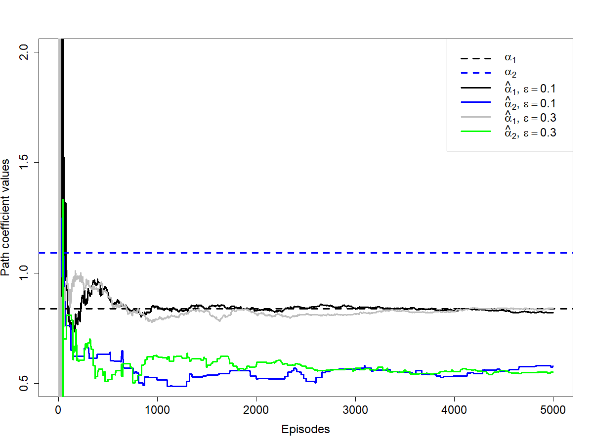
Estimating and above can be seen as an instance of the exploration/exploitation dilemma: In order to learn the effectiveness of the treatment administered by a particular doctor, the doctor has to administer the treatment to some patients, which leads to some patients receiving suboptimal treatment. A straightforward solution to this dilemma consists in combining exploration and exploitation as follows: Select the doctor with the highest effectiveness so far (i.e. exploitation) with probability , otherwise select the doctor at random (i.e. exploration). This strategy is called -greedy in the reinforcement learning community (Sutton and Barto 2018).
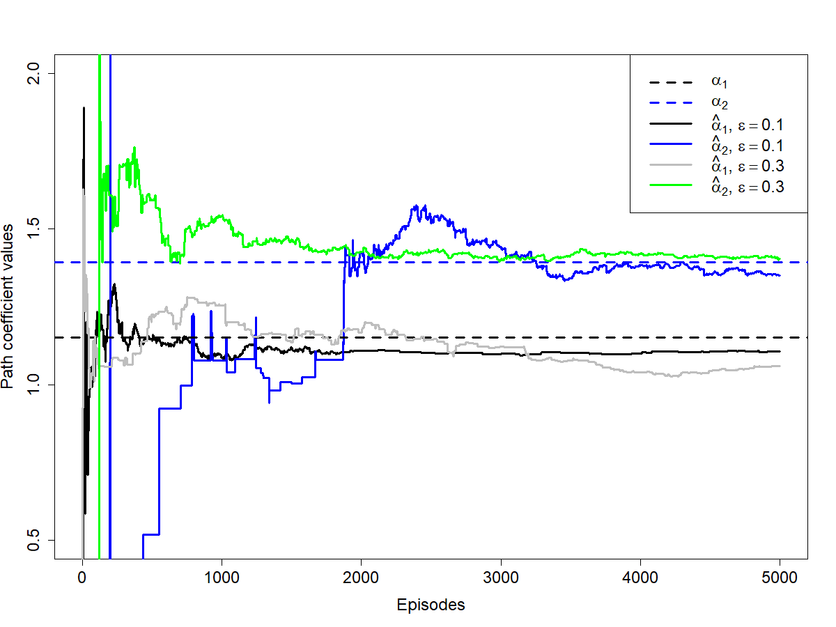
Figure 5 (top) shows the estimates of and (denoted as and ) obtained by running -greedy for 5000 iterations (a.k.a. episodes). Each episode consists in selecting a doctor for treating a patient. The doctor shares the data with us only if the treatment is regarded as ordinary. In our experiments, this means that each episode starts by choosing a doctor, say Doctor 1, according to the -greedy strategy. Then, a triplet of values is sampled from the corresponding linear structural equation model.33 3 Since negative abundance values do not make sense, if , or are negative then a new triplet is sampled. This seldom happens, anyway. Finally, the triplet is kept if and discarded otherwise. In the figure, we can clearly see that converges to , whereas does not converge to . Moreover, converges to a larger value than , which means that Doctor 1 is considered more effective than Doctor 2 and, thus, we should recommend the former. This is suboptimal because, as shown in the figure, is greater than and, thus, Doctor 2 should be preferred. This conclusion was consistent across many runs of the experiment. In each run, and were sampled uniformly from the intervals and respectively, i.e. Doctor 2 was more effective than Doctor 1. In each run, .
As discussed in Example 6, if we can estimate and , then we can correct the bias in . To illustrate this, assume that the doctors do not share with us data about individual extraordinary treatments but they do share aggregated data, in particular some estimates of and (which they can compute from all the ordinary and extraordinary treatments performed). Figure 5 (bottom) shows and when the correction is applied to the latter. We can appreciate that both path coefficient estimates converge to the true values, and that Doctor 2 is now preferred. Again, this conclusion was consistent across many runs of the experiment.
Of course, -greedy is not the only way of solving the problem above. Alternative solutions include Thompson sampling, upper confidence bound (UCB) or directly performing a randomized controlled trial. However, the conclusions should not differ essentially from the ones presented above. The code for our experiments is publicly available at https://www.dropbox.com/s/hawshrihhgr5uvi/MAB.zip?dl=0.
Appendix C: Suboptimal Decision Making II
In this appendix, we show that the bias introduced by adjusting for a faithful proxy of a confounder is negligible for decision making (recall Example 8). However, the bias may be substantial when adjusting for a proxy of a non-confounder in a confounding path, which may lead to suboptimal decision making. We do so with the help of the following fictitious but, in our opinion, realistic scenario. Doctor 1 and Doctor 2 both treat a certain disease by administering a dose of drug . The dose is determined by the abundance of in blood. The doctors use different methods to administer the drug, which we suspect affects the effectiveness of the drug. The effectiveness of the drug is assessed by measuring the abundance of Y in blood, which is determined by and . The lower the value of the higher the effectiveness of the treatment. Unwilling to disclose further details about the treatment, the doctors do not share with us any measurements of . However, they do provide us with measurements of two proxies of . Specifically, Doctor 1 provides us with the abundance of in blood, whereas Doctor 2 provides us with the abundance of in blood. The former is known to be caused by , whereas the latter is known to cause .44 4 Some authors would call a proxy and a driver.
In the language of path diagrams, the problem above can be stated as follows. We want to estimate in the following path diagram (Doctor 1) from a sample for , and :
We also want to estimate in the following diagram (Doctor 2) from a sample for , and :
Recall that is unobserved. As discussed in Example 8, if and are faithful proxies of , then the estimates of and should be close to and , respectively, which implies that we should be able to identify the optimal doctor. We illustrate this below with some experiments.
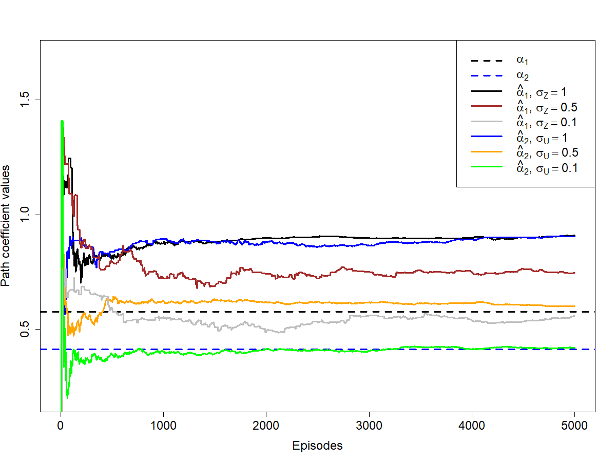
As in Appendix B, we use -greedy to solve the problem above. We consider and 5000 episodes. In each run of -greedy, and are sampled uniformly from the intervals and respectively, i.e. Doctor 2 is more effective than Doctor 1. The standard deviations of the error terms are all equal to 1, with the exception of the term corresponding to for Doctor 1 and the term corresponding to for Doctor 2. Specifically, . The smaller the values of and the better and are as proxies of . Figure 6 (top) shows a representative run of the many that we performed. We can see that Doctor 2 is preferred if and are equally good proxies of , i.e. . Moreover, both and converge to the true values when and are faithful proxies of , i.e. .
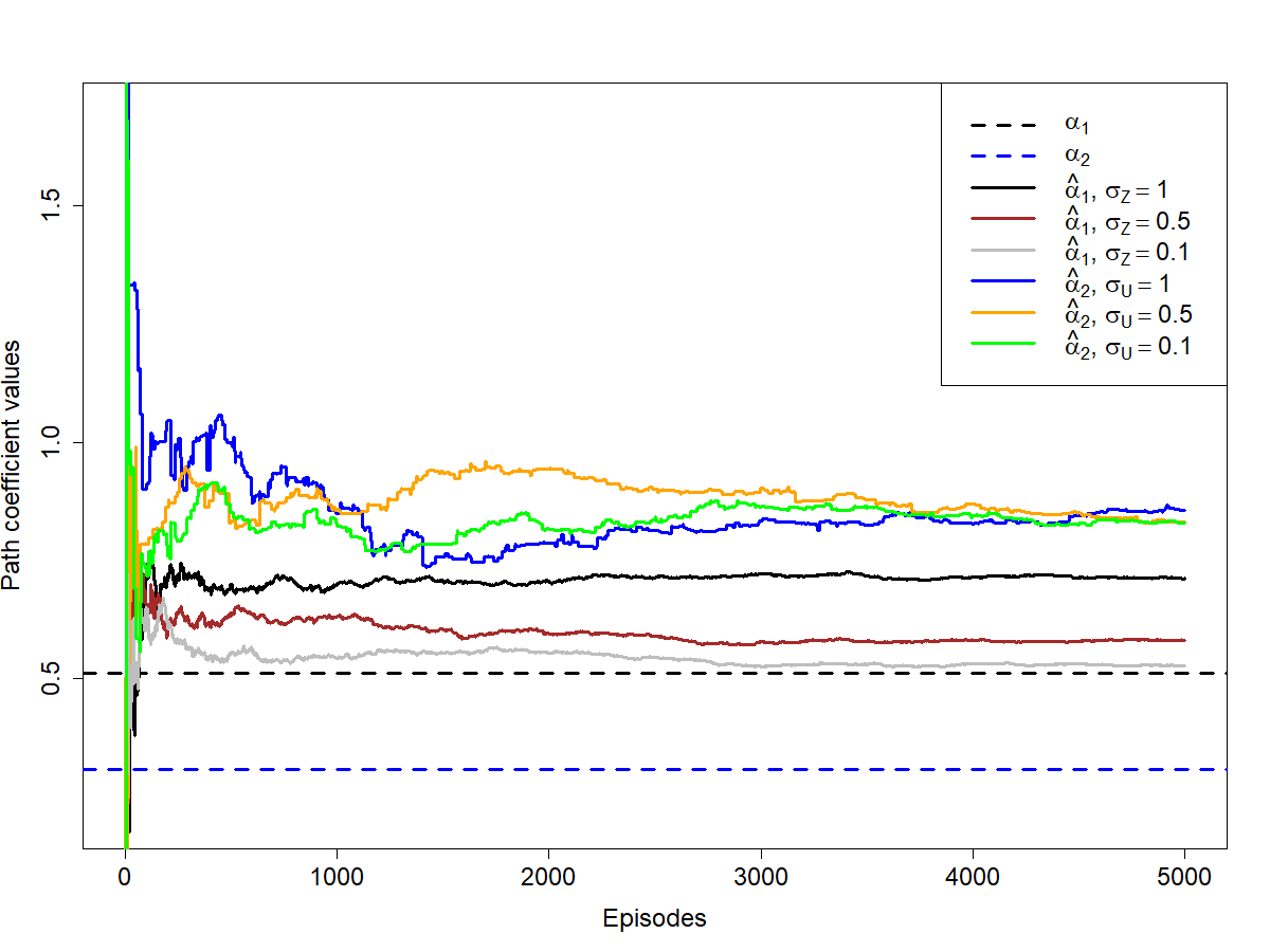
The experiments above may lead one to conclude that blocking a confounding path by adjusting for a proxy does not bias much the estimate of a causal effect as long as the proxy is a good one. However, this is not true. To illustrate it, we repeat the experiments above after replacing the confounding path from to in the path diagrams with the confounding path . Additional parameters are all set to 1. Figure 6 (bottom) shows a representative run of the new experiments. We can clearly see that converges to a smaller value than for every combination of and , i.e. no matter how good and are as proxies of . This means that Doctor 1 is considered more effective than Doctor 2 and, thus, that we should recommend the former. This is suboptimal because, as shown in the figure, is smaller than and, thus, Doctor 2 should be preferred. Note also that converges to when is almost a perfect proxy of . On the other hand, behaves bad no matter how good is as a proxy of . In summary, on the negative side, we wrongly recommend Doctor 1 but, on the positive side, we can estimate her effectiveness accurately if is a faithful proxy of . To get further insight into these results, we can repeat the reasoning in Example 8 now for the path diagrams of Doctor 1 and Doctor 2 after replacing the confounding path from to with the confounding path . Let denote the path diagram of Doctor 1. Since is singly-connected, we can apply Theorem 2 and conclude that . This implies that conditioning on reduces the covariance between and . Moreover, the greater the correlation between and , the greater the reduction and, thus, the closer comes to . Let now denote the path diagram of Doctor 2. Applying Theorem 2 to gives that . In other words, conditioning on leaves the covariance of and unchanged. Moreover, in and, thus, and, thus, . In other words, adjusting for does not solve our problem, even if is almost a perfect proxy of . In summary, the effectiveness of adjusting for a proxy depends on the type of confounding path, the type of causal relation between the proxy and the unobserved variable, and the correlation between them.
Appendix D: Beyond Singly-Connected Path Diagrams
In this appendix, we extend Theorems 2 and 3 from singly-connected diagrams to a superclass thereof. Note that we then only consider paths without colliders. The extension to path with colliders seems complicated.
In Section 2, we defined the separation criterion for path diagrams in terms of paths. For some of the results in this appendix, it is more convenient to define it in terms of routes. Recall that whereas all the nodes in a path must be different, the nodes in a route do not need to be so. Given a route from a node to a node in a path diagram, a node is a collider in if is a subroute of . Note that and may be the same node. Given a set of nodes , is said to be -open if
- •
every collider in is in , and
- •
ever non-collider in is outside .
Note that there is a -open route from to if and only if there is a -open path from to (see Lemma 21 in Appendix E). When such a path or route exists, we say that and are -connected.
Before presenting the results in this appendix, we define the operation of conditioning a path diagram on a node as replacing every edge with an edge , where is a new node. Note that is not removed. In terms of the associated system of linear equations, this implies (i) adding a new equation where is normally distributed with arbitrary mean and variance, and (ii) replacing every equation with an equation . Note that, after conditioning, we have that whereas and . See Figure 7 for an illustration. Let denote all the nodes in the path diagram at hand, and consider the distribution defined by the system of equations before conditioning on . This is the unnormalized conditional distribution of given . Let denote the new nodes created by conditioning on , and consider the distribution defined by the system of equations after conditioning on . This is the unnormalized conditional distribution of given . Note that both unnormalized conditional distributions coincide for all , i.e. for all and . Thus, their normalized versions coincide as well. So, computing partial covariances in either of them gives the same result, since partial covariances coincide with conditional covariances for Gaussian random vectors. In other words, the partial covariance in the original path diagram is equal to in the conditional diagram. Finally, we define conditioning on a set of nodes as conditioning on each node in . By the previous reasoning, the partial covariance in the original path diagram is equal to in the conditional diagram, where denotes the new nodes created by conditioning on . The following theorems show how to compute the latter. See the Appendix E for the proofs. We illustrate the theorems through some examples afterwards.
|
|
|
Theorem 16.
Consider a path diagram conditioned on a set of nodes . Let . Let denote all the -open paths from to . Suppose that no path in has colliders. Suppose that all the paths in have a subpath or . Suppose that there is no -open route with . Moreover, let and where
- •
is a subset of such that each is -connected to through by a path that does not contain any node that is in some path in except , and
- •
is a subset of such that each is -connected to through by a path that does not contain any node that is in some path in except .
Finally, let and suppose that or . Then,
Theorem 17.
Consider the same assumptions as in Theorem 16 with the only difference that all the paths in have now a subpath or or .55 5 In the third subpath type, the predecessor of does not have to be the same in every path in . It just has to reach through an edge or in every path in . Then,
Like Theorems 2 and 3, the two theorems above show that the partial covariance of two random variables can be computed by correcting their covariance with the product of some partial variance ratios. This implies that the partial covariance inherits the salient feature of factorizing over the nodes and edges in the paths between the two variables of interest. The two theorems above also imply that conditioning does not change the sign of the covariance, as stated in the following immediate corollary.
Corollary 18.
For the path diagrams that satisfy the conditions in Theorem 16 or 17, the corollary above implies that conditioning does not change the sign of the causal effect of on , and that Simpson’s paradox cannot occur.
|
|
|
We illustrate Theorem 16 with the following example.
Example 19.
Consider the path diagram to the left in Figure 8. Say that we want to compute with . The path diagram conditioned on can be seen to the right in Figure 8. Then, and . As discussed before, in the original diagram coincides with in the conditional diagram. Now, note that , , , , , and . Then, Theorem 16 gives
|
|
|
We illustrate Theorem 17 with the following example.
Example 20.
Consider the path diagram to the left in Figure 9. Say that we want to compute with . The path diagram conditioned on can be seen to the right in Figure 9. Then, and . As discussed before, in the original diagram coincides with in the conditional diagram. Now, note that , , and . Then, Theorem 17 gives
|
|
|
Theorems 16 and 17 can be extended to when all the paths from to in the conditional path diagram share more than one subpath. For instance, consider the path diagram to the left in Figure 10. Say that we want to compute with . The path diagram conditioned on can be seen to the right in Figure 10. Then, and . As discussed before, in the original diagram coincides with in the conditional diagram. Now, note that , , , , , and . Note also that the conditional diagram has two -open paths from to , which share two subpaths: and . Therefore, neither Theorem 16 nor 17 applies. However, applying Theorem 16 followed by Theorem 17 gives
| (5) |
The proof of correctness of the previous expression is simply a concatenation of the proofs of Theorems 16 and 17. We omit the details. An alternative way of answering the previous query is by first absorbing the subpath into the subpath . Now, there is only one shared subpath in the path diagram conditioned on , namely . Then, Theorem 16 gives Equation 5. This absorption trick is always possible when there are several shared subpaths. We omit the details.
Appendix E: Proofs of Appendix D
We start with some lemmas stating some auxiliary results. Recall from Footnote 5 that when we say that every path has a subpath , we do not mean that the successor of is the same in every path. We mean that the successor is reached through an edge or in every path. Given a route from to , we let denote the subroute of from to . Given two routes and , we let denote the route from to resulting from concatenating and . Finally, the path corresponding to a -open route from to is a -open path from to whose edges are a subset of the edges in the route. Such a path always exists by Lemma 21.
Lemma 21.
There is a -open route from to if and only if there is a -open path from to . Moreover, the path and the route can be chosen such that the edges in the former are a subset of the edges in the latter.
Proof.
Let be a -open path from to . For every subpath of such that , do the following. First, find a path with and . Such a path must exist for to be -open. Second, replace with . The result is the desired route.
Let be a -open route from to . Repeat the following two steps while possible. The result is the desired path. First, choose a node that occurs several times in . Let and denote the first and the last occurrences of in . Assume without loss of generality that no node in occurs in except . Second, consider the following cases.
- •
If is , then replace it with .
- •
If is , then replace it with .
- •
If is , then replace it with . Note that or some descendant of must be in for the original to be -open.
∎
Lemma 22.
Consider a path diagram. Let , , and be nodes and a set of nodes. If and and , then
Proof.
Note that implies that
which implies that where . Likewise, implies that where . Likewise, implies that . Therefore,
∎
Lemma 23.
Consider a path diagram. Let , and be nodes and a set of nodes. If , then
Proof.
Note that implies that
which implies that
Therefore,
∎
Lemma 24.
Consider a path diagram. Let , and be nodes and a set of nodes. If or , then .
Proof.
Note that and imply and , respectively. Thus, if or then
∎
Lemma 25.
Consider a path diagram. Let denote all the -open paths from to . Suppose that no path in has colliders. Suppose that all the paths in have a subpath or . Let be a node that is -connected to by a path that does not contain any node that is in some path in except . If , then
Proof.
Consider first the case where is a subpath of every path in . Assume to the contrary that and let be a -open route. Follow until reaching or , and let .
- •
If is reached first, then consider the first occurrence of in and note that is a -open route. Moreover, it does not contain any edge that is in some path in because, otherwise, contains the edge ( cannot by definition) and, thus, it is not -open. Then, the path corresponding to contradicts the assumptions in the lemma.
- •
If is reached first, then let denote a -open path that does not contain any node that is in some path in except . Such a path exists by the assumptions in the lemma. Thus, is a -open route, because neither nor is a collider in it. The latter follows from the assumption that . Moreover, the route does not contain any edge that is in some path in because, otherwise, contains the edge ( and cannot by definition) and thus it reaches first. Then, the path corresponding to contradicts the assumptions in the lemma.
Consequently, . We can analogously prove that . Now, assume to the contrary that and let be a -open route. Note that must be in because, otherwise, is -open and, thus, its corresponding path contradicts the assumptions in the lemma. Consider the first occurrence of in , and let . Then, is a -open route. Moreover, the route does not contain any edge that is in some path in because, otherwise, contains the edge ( cannot by definition) and thus it is not -open. Then, the path corresponding to contradicts the assumptions in the lemma. Consequently, . Therefore, the desired result follows from Lemma 22.
Finally, consider the case where is a subpath of every path in . Assume to the contrary that and let be a -open route. Follow until reaching or .
- •
If is reached first, then note that does not contain any edge that is in some path in because, otherwise, is not -open. Then, the path corresponding to contradicts the assumptions in the lemma.
- •
If is reached first, let denote a -open path that does not contain any node that is in some path in except . Such a path exists by the assumptions in the lemma. Then, is a -open route, because is not a collider in it due to the assumption that . Moreover, the route does not contain any edge that is in some path in because, otherwise, contains the edge ( cannot by definition) and thus reaches first. Then, the path corresponding to contradicts the assumptions in the lemma.
Consequently, and, thus, the desired result follows from Lemma 23. ∎
Lemma 26.
Consider a path diagram. Let denote all the -open paths from to . Suppose that no path in has colliders. Suppose that all the paths in have a subpath or . Let be a node that is -connected to by a path that does not contain any node that is in some path in except . If and are all the -open paths from to , then
Proof.
Consider first the case where is a subpath of every path in . Assume to the contrary that and let be a -open route. Follow until reaching or , and let .
- •
If is reached first, then consider the first occurrence of in and note that is a -open route. Moreover, it does not contain any edge that is in some path in because, otherwise, contains the edge ( cannot by definition) and, thus, it is not -open. Then, the path corresponding to contradicts the assumptions in the lemma.
- •
If is reached first, then let denote a -open path that does not contain any node that is in some path in except . Such a path exists by the assumptions in the lemma. Thus, is a -open route from to , because is a collider in it whereas is not. The former follows from the assumption that . Moreover, the route does not contain any edge that is in some path in because, otherwise, contains the edge ( and cannot by definition) and thus it reaches first. Then, the path corresponding to contradicts the assumptions in the lemma.
Consequently, . We can analogously prove that . Now, assume to the contrary that and let be a -open route. Note that must be in because, otherwise, is -open and, thus, its corresponding path contradicts the assumptions in the lemma. Consider the first occurrence of in , and let . Then, is a -open route. Moreover, the route does not contain any edge that is in some path in because, otherwise, contains the edge ( cannot by definition) and thus it is not -open. Then, the path corresponding to contradicts the assumptions in the lemma. Consequently, . Therefore, the desired result follows from Lemma 22.
Finally, consider the case where is a subpath of every path in . Assume to the contrary that and let be a -open route. Follow until reaching or .
- •
If is reached first, then note that does not contain any edge that is in some path in because, otherwise, is not -open. Then, the path corresponding to contradicts the assumptions in the lemma.
- •
If is reached first, let denote a -open path that does not contain any node that is in some path in except . Such a path exists by the assumptions in the lemma. Then, is a -open route, because is a collider in it due to the assumption that . Moreover, the route does not contain any edge that is in some path in because, otherwise, contains the edge ( cannot by definition) and thus reaches first. Then, the path corresponding to contradicts the assumptions in the lemma.
Consequently, and, thus, the desired result follows from Lemma 23. ∎
Lemma 27.
Consider a path diagram. Let denote all the -open paths from to . Suppose that no path in has colliders. Suppose that all the paths in have a subpath or . Let be a node that is -connected to through by a path that does not contain any node that is in some path in except . If and is not -connected to through , then
Proof.
Consider first the case where is a subpath of every path in . Assume to the contrary that and let be a -open route. Follow until reaching or , and let .
- •
If is reached first, then consider the first occurrence of in and note that ends with an edge because, otherwise, is a -open route that has a subroute and, thus, its corresponding path contradicts the assumptions in the lemma. Then, must start with an edge for to be -open. However, this contradicts the assumption that is not -connected to through .
- •
If is reached first, then let denote a -open path that does not contain any node that is in some path in except . Such a path exists by the assumptions in the lemma. Thus, is a -open route, because neither nor is a collider in it. The latter follows from the assumption that . Moreover, the route does not contain any edge that is in some path in because, otherwise, contains the edge ( and cannot by definition) and thus it reaches first. Then, the path corresponding to contradicts the assumptions in the lemma.
Consequently, . When is a subpath of every path in , we can prove that much in the same way. Consequently, in either case and, thus, the desired result follows from Lemma 24. ∎
Lemma 28.
Consider a path diagram. Let denote all the -open paths from to . Suppose that no path in has colliders. Suppose that all the paths in have a subpath or . Let be a node that is -connected to through by a path that does not contain any node that is in some path in except . If , and is not -connected to through , and are all the -open paths from to , then
Proof.
Consider first the case where is a subpath of every path in . Assume to the contrary that and let be a -open route. Follow until reaching or , and let .
- •
If is reached first, then consider the first occurrence of in and note that ends with an edge because, otherwise, is a -open route that has a subroute and, thus, its corresponding path contradicts the assumptions in the lemma. Then, must start with an edge for to be -open. However, this contradicts the assumption that is not -connected to through .
- •
If is reached first, then let denote a -open path that does not contain any node that is in some path in except . Such a path exists by the assumptions in the lemma. Thus, is a -open route, because is a collider in it whereas is not. The former follows from the assumption that . Moreover, the route does not contain any edge that is in some path in because, otherwise, contains the edge ( and cannot by definition) and thus it reaches first. Then, the path corresponding to contradicts the assumptions in the lemma.
Consequently, . When is a subpath of every path in , we can prove that much in the same way. Consequently, in either case and, thus, the desired result follows from Lemma 24. ∎
Lemma 29.
Consider a path diagram. Let denote all the -open paths from to . Suppose that no path in has colliders. Suppose that all the paths in have a subpath or . Let be a node that is -connected to through by a path that does not contain any node that is in some path in except . If and is not -connected to through , then
Proof.
Consider first the case where is a subpath of every path in . Assume to the contrary that and let be a -open route. Follow until reaching or , and let .
- •
If is reached first, then note must be a collider in for this to be -open. However, the last occurrence of in contradicts the assumption that is not -connected to through .
- •
If is reached first, then let denote a -open path that does not contain any node that is in some path in except . Such a path exists by the assumptions in the lemma. Thus, is a -open route, because neither nor is a collider in it. The latter follows from the assumption that . Moreover, the route does not contain any edge that is in some path in because, otherwise, contains the edge ( and cannot by definition) and thus it reaches first. Then, the path corresponding to contradicts the assumptions in the lemma.
Consequently, . Now, assume to the contrary that and let be a -open route. Follow until reaching or , and let .
- •
If is reached first, then note must be a collider in for this be -open. However, the last occurrence of in contradicts the assumption that is not -connected to through .
- •
If is reached first, then let denote a -open path that leaves through and that does not contain any node that is in some path in except . Such a path exists by the assumptions in the lemma. Thus, is a -open route, because neither nor is a collider in it. The latter follows from the assumption that . Moreover, the route does not contain any edge that is in some path in because, otherwise, contains the edge ( and cannot by definition) and thus reaches first. Then, the path corresponding to contradicts the assumptions in the lemma.
Consequently, . Now, assume to the contrary that and let be a -open path. Note that must be a collider or a descendant of a collider in because, otherwise, is not in and, thus, is -open, which contradicts the assumptions in the lemma. Note also that the assumption that is -connected to through implies that some descendant of is in . Actually, some descendant of must be in due to the assumption that . Then, is -open, which contradicts the assumptions in the lemma. Consequently, . Therefore, the desired result follows from Lemma 22.
Finally, consider the case where is a subpath of every path in . Assume to the contrary that and let be a -open route. Follow until reaching or .
- •
If is reached first, then note must be a collider in for this to be -open. However, the last occurrence of in contradicts the assumption that is not -connected to through .
- •
If is reached first, let denote a -open path that does not contain any node that is in some path in except . Such a path exists by the assumptions in the lemma. Then, is a -open route, because is not a collider in it due to the assumption that . Moreover, the route does not contain any edge that is in some path in because, otherwise, contains the edge ( cannot by definition) and thus it reaches first. Then, the path corresponding to contradicts the assumptions in the lemma.
Consequently, and, thus, the desired result follows from Lemma 23. ∎
Lemma 30.
Consider a path diagram. Let denote all the -open paths from to . Suppose that no path in has colliders. Suppose that all the paths in have a subpath or . Let be a node that is -connected to through by a path that does not contain any node that is in some path in except . If , and is not -connected to by any path that reaches through , and are all the -open paths from to , then
Proof.
Consider first the case where is a subpath of every path in . Assume to the contrary that and let be a -open route. Follow until reaching or , and let .
- •
If is reached first, then note that must be a collider in for this to be -open. However, the last occurrence of in contradicts the assumption that is not -connected to through .
- •
If is reached first, then let denote a -open path that does not contain any node that is in some path in except . Such a path exists by the assumptions in the lemma. Thus, is a -open route, because is a collider in it whereas is not. The former follows from the assumption that . Moreover, the route does not contain any edge that is in some path in because, otherwise, contains the edge ( and cannot by definition) and thus it reaches first. Then, the path corresponding to contradicts the assumptions in the lemma.
Consequently, . Now, assume to the contrary that and let be a -open route. Follow until reaching or , and let .
- •
If is reached first, then note that must be a collider in for this to be -open. However, the last occurrence of in contradicts the assumption that is not -connected to through .
- •
If is reached first, then let denote a -open path that leaves through and that does not contain any node that is in some path in except . Such a path exists by the assumptions in the lemma. Thus, is a -open route, because is a collider in it whereas is not. The former follows from the assumption that . Moreover, the route does not contain any edge that is in some path in because, otherwise, contains the edge ( and cannot by definition) and thus reaches first. Then, the path corresponding to contradicts the assumptions in the lemma.
Consequently, . Now, assume to the contrary that and let be a -open path. Note that must be a collider or a descendant of a collider in because, otherwise, is not in and, thus, is -open, which contradicts the assumptions in the lemma. Note also that the assumption that is -connected to through implies that some descendant of is in . Then, is -open, which contradicts the assumptions in the lemma. Consequently, . Therefore, the desired result follows from Lemma 22.
Finally, consider the case where is a subpath of every path in . Assume to the contrary that and let be a -open route. Follow until reaching or .
- •
If is reached first, then note must be a collider in for this to be -open. However, the last occurrence of in contradicts the assumption that is not -connected to through .
- •
If is reached first, let denote a -open path that does not contain any node that is in some path in except . Such a path exists by the assumptions in the lemma. Then, is a -open route, because is a collider in it due to the assumption that . Moreover, the route does not contain any edge that is in some path in because, otherwise, contains the edge ( cannot by definition) and thus it reaches first. Then, the path corresponding to contradicts the assumptions in the lemma.
Consequently, and, thus, the desired result follows from Lemma 23. ∎
Proof of Theorem 16.
Consider hereinafter the path diagram conditioned on . We first compute from by adding the nodes in to the conditioning set in the order . The assumption that are all the -open paths from to implies that are all the -open paths from to because, otherwise, any other path cannot be closed afterwards which contradicts the assumption. To see it, note that a node does not close any open path, since there is no subpath or due to the conditioning operation. Then,
by Lemma 25 if , or Lemma 26 if . Likewise,
by Lemma 25 or 26. Combining the last two equations gives
Continuing with this process for the rest of the nodes in gives
| (6) |
Now, we compute from by adding the nodes in to the conditioning set in the order . Recall from above that are all the -open paths from to . Then,
by repeating the reasoning that led to Equation 6. Moreover, combining the last two equations yields
| (7) |
Now, we compute from by adding the nodes in to the conditioning set in the order . The assumption that there is no -open route implies that there is no -open path from to through . To see it, assume the opposite. Then, there are -open paths from to through both and . This implies that there is a route that contains , and the route is -open or -open. Then, there is a path that is -open or -open by Lemma 21. However, this path cannot be closed afterwards which contradicts the assumption. To see it, note that a node does not close any open path, since there is no subpath or due to the conditioning operation. Consequently, there is no -open path from to through . Recall also from above that are all the -open paths from to . Then,
by Lemma 27 if , or Lemma 28 if . Likewise,
by Lemma 27 or 28. Combining the last two equations gives
Continuing with this process for the rest of the nodes in gives
| (8) |
Now, we compute from by adding the nodes in to the conditioning set in the order . Recall from above that are all the -open paths from to . Recall also from above that the assumption that there is no -open route implies that there is no -open path from to through . Then,
by repeating the reasoning that led to Equation 6 but using Lemmas 29 and 30 instead. Moreover, combining the last equation with Equations 7 and 8 gives
Finally, continuing with the process above for yields
which implies the desired result by repeated application of Lemma 24. ∎
References
- Anderson (2003) T. W. Anderson. An Introduction to Multivariate Statistical Analysis. Wiley, 2003.
- Chaudhuri (2005) S. Chaudhuri. Using the Structure of d-Connecting Paths as a Qualitative Measure of the Strength of Dependence. PhD thesis, University of Washington, 2005.
- Chaudhuri (2014) S. Chaudhuri. Qualitative Inequalities for Squared Partial Correlations of a Gaussian Random Vector. Annals of the Institute of Statistical Mathematics, 66:345–367, 2014.
- Chaudhuri and Richardson (2003) S. Chaudhuri and T. Richardson. Using the Structure of d-Connecting Paths as a Qualitative Measure of the Strength of Dependence. In Proceedings of the 19th Conference on Uncertainty in Artificial Intelligence, pages 116–123, 2003.
- Chaudhuri and Tan (2010) S. Chaudhuri and G. L. Tan. On Qualitative Comparison of Partial Regression Coefficients for Gaussian Graphical Markov Models. In Algebraic Methods in Statistics and Probability II. Contemporary Mathematics, Vol. 516, pages 125–133. American Mathematical Society, 2010.
- Ong (2014) V. M. H. Ong. Model Selection for Graphical Markov Models. PhD thesis, National University of Singapore, 2014.
- Pearl (2009) J. Pearl. Causality: Models, Reasoning, and Inference. Cambridge University Press, 2009.
- Pearl (2013) J. Pearl. Linear Models: A Useful “Microscope” for Causal Analysis. Journal of Causal Inference, 1:155–170, 2013.
- Pearl (2014) J. Pearl. Comment: Understanding Simpson’s Paradox. The American Statistician, 68:8–13, 2014.
- Studený (2005) M. Studený. Probabilistic Conditional Independence Structures. Springer, 2005.
- Sutton and Barto (2018) R. S. Sutton and A. G. Barto. Reinforcement Learning: An Introduction. The MIT Press, 2018.
- Wright (1921) S. Wright. Correlation and Causation. Journal of Agricultural Research, 20:557–585, 1921.