On the Secrecy Performance Over $\mathrm{N}$-Wave with Diffuse Power Fading Channel

The fifth-generation (5G) of mobile networks aims to raise the capacity and performance of communication systems to unprecedented levels, including ultra-high data rates, ultra-wide radio coverage, massive simultaneously connected devices and ultra-low latencies. The new scenarios of wireless systems under the umbrella of 5G include mm-Wave, device-to-device, machine-type, and vehicular communications, among many others [1]. In particular, recent investigations have shown that none of the well-established fading models (e.g., Rayleigh, Rician and Nakagami-$m$) present accurate fit with field measurements in mm-Wave communications [2]. One of the reasons for such mismatch relies in the fact that classical fading models heavily rely on the central limit theorem (CLT), which assumes a sufficiently large number of multipath waves arriving at the receiver ends – and such conditions are not always met [3].

In the last years, some efforts have been oriented to formulate more accurate channel models that overcome such limitation. Among them, stochastic fading models that explicitly discern between the individual multipath waves classically regarded as line-of-sight (LOS) components have been proposed as a way for bridging the gap between CLT-based approaches and purely ray-based models. Durgin’s two-wave with diffuse power (TWDP) [4] and its generalization in [5] are known to improve the fit to field measurements in different scenarios including mm-Wave set-ups [2, 6], compared to conventional small-scale fading models.

On the other hand, a myriad of challenges must still be overcome so that 5G converges into a reliable, safe and efficient system. One of the most critical aspects is related to the security of information transmission, given that 5G is designed to support rather diverse applications. As a consequence, highly confidential and vulnerable data is expected to be transmitted in future 5G and beyond networks, which because of their wireless nature are sensitive to eavesdropping. Regarding this, physical layer security (PLS) [7] emerges as a promising solution to complement traditional security systems by taking advantage of the random nature of wireless channels to provide lightweight and efficient solutions for increasing the security level in some applications [8, 9].

The physical layer security performance in wireless channels is a rather well-investigated topic in the literature. Nevertheless, because of the intricate nature of physically-motivated wireless fading models, available results are restricted to some special cases [11, 10] on which only two specular components are considered. Very recently, it was suggested in [12] that the inability to achieve perfect secrecy in wireless channels was an artifact due to the consideration of the CLT assumption. Hence, the impact of the number of multipath waves arriving at the receiver ends, as well as their relative amplitudes, has a dramatical effect on the secrecy performance. However, the results in [12] considered only the limit case of a total absence of diffuse fading, and the derivation of analytical expressions for the secrecy performance metrics was not possible for a an arbitrary number of waves.

In this paper, we investigate the PLS performance in a wireless set-up, by assuming that the received signal is built from the superposition of an arbitrary number $\mathrm{N}$ of dominant multipath waves, plus some additional diffuse components – this will be referred to as $\mathrm{N}$-wave with diffuse power (NWDP) fading, for which some formulations have been recently proposed in order to deal with its rather unwieldy nature [13, 14]. Our goal is to perform a fine-grain characterization of the role of individual multipath waves on the secrecy performance, and to support our findings with analytical results. We derive exact expressions for the secrecy outage probability (SOP) for an arbitrary number of dominant waves at the desired and eavesdropping ends, as well as simplified approximations that become asymptotically tight in the high signal-to-noise ratio (SNR) regime. Some useful insights for improving the secrecy performance in this scenario will be derived, which are inherently linked to the underlying propagation mechanisms and characteristics captured by the NWDP fading model. The main contributions of this paper are as follows:

• •

  An exact closed-form expression for the SOP in terms of well-know functions for the classical Wyner’s channel model under NWDP fading.

• •

  A high SNR approximation of the SOP is also derived, which can be used straightforwardly in the context of PLS. The merits of such expression are: $(i)$ when $\overline{\gamma}_{\mathrm{E}}$ is at high SNR regime, it is highly tight to the exact SOP; $(ii)$ it notably reduces the computational effort concerning the exact SOP. This fact helps to the wireless system designers when requiring quick evaluation of security risks.

• •

  Some useful insights into the system are also provided through the asymptotic analysis based on the exact analytical expression of the SOP.

The remainder of this paper is organized as follows. System and channel models are described in Section II. Section III derives closed-form expressions for $(i)$ the SOP; $(ii)$ a high SNR regime of the SOP; $(iii)$ the asymptotic behaviour of the SOP over NWDP fading channel. Section IV shows illustrative numerical results and discussions. Finally, concluding remarks are provided in Section V.

Notation: Throughout this paper, $f_{(Z)}(z)$ and $F_{(Z)}(z)$ denote the probability density function (PDF) and the cumulative distribution function (CDF) of a random variable $Z$. $\mathbb{E}\left[\cdot\right]$ denotes expectation, $\Pr\left\{\cdot\right\}$ denotes probability, and $\lvert\cdot\rvert$ denotes the absolute value. In addition, $L_{n}(\cdot)$ denotes the Laguerre polynomial [15, Eq. (22.2.13)], $\Gamma(\cdot)$ denotes the gamma function [15, Eq. (6.1.1)]; $\gamma(\cdot,\cdot)$, the lower incomplete gamma function [15, Eq. (6.5.2)]; ${}_{2}F_{1}\left(\cdot,\cdot;\cdot;\cdot\right)$, denotes the hypergeometric function [15, Eq. (15.1.1)], and $\left(\cdot\right)_{\left(\cdot\right)}$ is the Pochhammer symbol [15, Eq. (6.1.222)].

We consider the classic Wyner’s wiretap channel as depicted in Fig. 1, where a legitimate transmitter Alice ($\mathrm{A}$) sends confidential messages to the legitimate receiver Bob ($\mathrm{B}$) through the main channel, while the eavesdropper Eve ($\mathrm{E}$) tries to intercept these messages from its received signal over the eavesdropper channel. It is assumed that the main and eavesdropper channels experience independent quasi-static fading. Without loss of generality, we assume that all nodes are equipped with a single antenna.

We express the signal at each of the receiving ends as a superposition of $\mathrm{N}$ multipath waves arising from dominant specular reflections, and $M$ additional waves associated to diffuse scattering:

Because each diffuse scatterer is able to generate several multipath waves [16], we can safely assume that $M\rightarrow\infty$ and hence the diffuse component¹¹ 1 We note that the consideration of arbitrary $N$ in (1) allows for individually accounting for the effect of having multiple specular waves and largely differs from the conventional assumptions in fading modeling, reducing only for $N=0,1,2$ to the Rayleigh, Rician and TWDP cases, respectively [4]. tends to be Gaussian distributed, i.e., $\sum_{k=1}^{M}V_{k}\exp\left({\mathrm{j}\theta_{k}}\right)\approx V_{d}\exp\left({\mathrm{j}\theta_{d}}\right)$, so that $V_{d}$ is Rayleigh distributed with $\mathbb{E}\{|V_{d}|^{2}\}=2\sigma^{2}=\Omega$.

In (1), $V_{i}\exp(\mathrm{j}\theta_{i})$ denotes the $i$-$th$ specular component having a constant amplitude $V_{i}$ and a uniformly distributed random phase $\theta_{i}\sim\mathcal{U}[0,2\pi)$. The random phases for each dominant wave are assumed to be statistically independent.

Let $\gamma\stackrel{{\scriptstyle\Delta}}{{=}}\gamma_{0}\mathrm{R}^{2}$ be the instantaneous received SNR through, where $\gamma_{0}\stackrel{{\scriptstyle\Delta}}{{=}}P_{\mathrm{T}}/N_{0}$ is defined as the transmit SNR, with $P_{\mathrm{T}}$ being the transmit power and $N_{0}$ being the mean power of the additive white Gaussian noise. Note that $\gamma$ can also be redefined for the sake of convenience as $\gamma=\overline{\gamma}|h|^{2}$, where $h$ denotes any normalized fading channel, i.e., $\mathbb{E}\{|h|^{2}\}=1$ and $\overline{\gamma}$ representing the average receive SNR. According to the formulation in [13], the corresponding PDF and CDF of $\gamma$ over NWDP fading channel are:

where $i\in\left\{\mathrm{B},\mathrm{E}\right\}$ represents either the main channel or the eavesdropper channel, $\overline{\gamma}_{i}$ is the average receive SNR at $\mathrm{B}$ or $\mathrm{E}$ as previously stated, i.e.,

where $\eta_{i}$ is the path-loss exponent, and $r_{i}$ is the propagation distance²² 2 Here, as in the LOS ball blockage model, we assume that $r_{i}$ lies within a sphere of fixed radius $R_{\mathrm{B}}$. Interested readers can revise [18] for further guidance about simplification of the LOS region as a fixed equivalent LOS ball in mm-Wave cellular networks.. The $C_{n_{i}}$ coefficient can be calculated recursively by [13]

where $\epsilon_{i}=\left(\mathbb{E}\left[R_{i}^{2}\right]\right)^{-1}$, and

where the initial value is $u_{1}^{2k_{i}}=v_{1}^{2k_{i}}$, and

In this section, we validate the accuracy of the proposed expressions⁵⁵ 5 Here, it is worth mentioning that depending on the value of the involved channel parameters, these series require different number of terms to attain an accurate approximation. In this context, the overall convergence speed of these series is achieved faster for small values of both dominant rays (e.g, $\mathrm{N}_{\mathrm{B}}$, and $\mathrm{N}_{\mathrm{E}}$) and power of Bob’s dominant specular components (i.e., $K_{\mathrm{dB}}^{\mathrm{B}}$). For instance, exhaustive tests have shown that the number of terms to arrive at the desired accuracy (e.g., $10^{-6}$) varied from 20 to 30 at Bob and from 4 to 10 at Eve, and the average elapsed times to obtain the aforementioned accuracy were $\sim 14.1,27.5,81.7,103.5,114.6$ seconds for $\mathrm{N}=1,\dots,5$, respectively. Moreover, the mathematical representation of the derived series consists of well-known elementary and special functions, which can be easily implemented in software for numerical evaluation.. for some representative cases via Monte Carlo simulations. We define a power ratio parameter similar to the well-known Rician $K$ parameter, e.g., $K_{\mathrm{N}_{i}}\mathrel{\mathop{\kern 0.0pt=}\limits^{\Delta}}\frac{\Omega_{\mathrm{N}_{i}}}{\Omega_{i}}$, with $\Omega_{\mathrm{N}_{i}}=\sum_{n=0}^{\mathrm{N}_{i}}V_{n,i}^{2}$ being the total average power of the specular components. For the sake of comparison, the Rayleigh case (i.e., $\mathrm{N}_{\mathrm{B}}=\mathrm{N}_{\mathrm{E}}=0$) is included as a reference.

Before getting into the numerical examples, an important remark is in order. Herein, we emphasize on providing clear evidence to identify the impact of increasing/decreasing both the number and the power of the dominant specular waves over the secrecy performance. In other words, we aim to determine to what extent it is worth that each of the individual specular waves is treated separately, or it can be safely incorporated into the diffuse component.

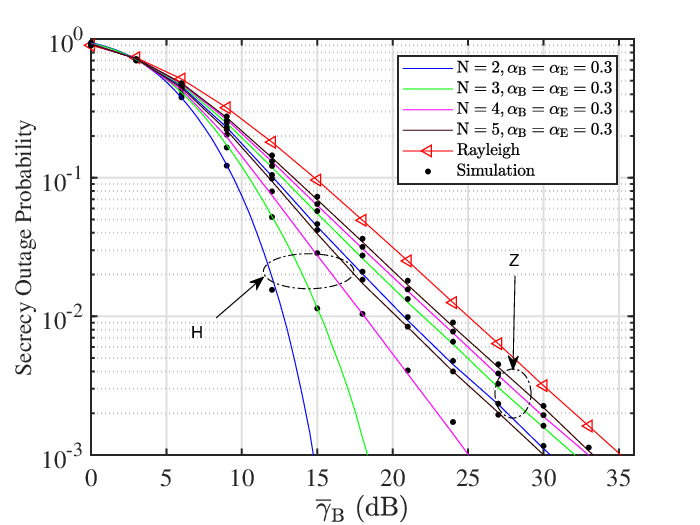
In Fig. 2, we compare the SOP as a function of $\overline{\gamma}_{\mathrm{B}}$ for different values of dominant specular components $\mathrm{N}_{\mathrm{B}}=\mathrm{N}_{\mathrm{E}}=\mathrm{N}$, by considering the case of balanced amplitudes, i.e., $V_{n,\mathrm{B}}=V_{n,\mathrm{E}}$ $\forall\mathrm{B}$, $n=1\dots\mathrm{N}$. For this scenario, the corresponding fading parameters are given by: $K_{\mathrm{dB}}^{\mathrm{B}}=10\log_{10}\left(K_{\mathrm{B}}=K_{\mathrm{N}_{\mathrm{B}}}\right)\in\left\{8,25\right\}$ dBs with $K_{\mathrm{dB}}^{\mathrm{E}}=0$ dB, $R_{\mathrm{S}}$ = 1 bps/Hz, and $\overline{\gamma}_{\mathrm{E}}=1$ dB. Note that in all instances, Monte Carlo simulations perfectly match with our derived results.

We see that the secrecy performance does not monotonically increase with the number of specular components; instead, we see that the cases with $\mathrm{N}_{\mathrm{B}}=1$ and $\mathrm{N}_{\mathrm{B}}=2$ bound the secrecy performance when the rest of parameters are fixed. This is in coherence with the fact that for an even number of dominant specular components of equal amplitudes, the probability of total cancellation between them is larger than when an odd number is considered [17]. This increases fading severity for the desired link more relevantly for large $K$, which ultimately degrades the SOP. We also see that for $\mathrm{N}=4$, the performance is very similar than in the Rayleigh case (i.e., $\mathrm{N}\rightarrow\infty$).

In Fig. 3, we now evaluate the SOP vs. $\overline{\gamma}_{\mathrm{B}}$ for different numbers of dominant specular components $\mathrm{N}_{\mathrm{B}}=\mathrm{N}_{\mathrm{E}}=\mathrm{N}$ by considering an unbalanced amplitudes scenario. For simplicity, yet without loss of generality, the amplitudes of successive rays are expressed in terms of the amplitude of the first dominant component, as proposed in [12], that is, $V_{n,i}=\alpha_{n,i}V_{1,i}$ for $n=2,\dots,\mathrm{N}_{i}$, with $0<\alpha_{n,i}<1$ and $i$ $\in\left\{\mathrm{B},\mathrm{E}\right\}$. Considering this, we set: $\alpha_{n,i}=\alpha_{\mathrm{B}}=\alpha_{\mathrm{E}}=0.3$ with $K_{\mathrm{dB}}^{\mathrm{B}}\in\left\{8,25\right\}$ dBs, $K_{\mathrm{dB}}^{\mathrm{E}}=0$ dB, $R_{\mathrm{S}}$ = 1 bps/Hz, and $\overline{\gamma}_{\mathrm{E}}=1$ dB. Here, we investigate the impact of increasing both the number and the power of Bob’s dominant rays for the case of unbalanced amplitudes. We observe in all traces that, unlike on the balanced counterpart, the SOP performance now monotonically improves when rising $K_{\mathrm{dB}}^{\mathrm{B}}$ or lowering $\mathrm{N}$, regardless of whether it is even or odd. It can be observed that a reduced number of dominant specular components at Bob is now beneficial from a secrecy perspective. We also see that in all cases, the SOP performance is always better than its Rayleigh counterpart. Regarding the asymptotic behaviour, it can be noticed that the asymptotic plots accurately approximate the SOP curves at high SNR regime. Additionally, all curves have different slopes. The reason for this will be discussed later.

In Fig. 4, we evaluate both the SOP and the $\text{SOP}_{\text{A}}$ as a function of $\overline{\gamma}_{\mathrm{B}}$, in order to understand the interplay between the number of dominant specular components $\mathrm{N}_{\mathrm{B}}=\mathrm{N}_{\mathrm{E}}=\mathrm{N}$, the amplitude imbalance and the power of the dominant components. We use a similar set of parameters as those in Fig. 3, except for $\left\{\alpha_{\mathrm{B}},\alpha_{\mathrm{E}}\right\}=\left\{0.2,0.9\right\}$, $\left\{\alpha_{\mathrm{B}},\alpha_{\mathrm{E}}\right\}=\left\{0.9,0.2\right\}$, and $\overline{\gamma}_{\mathrm{E}}=8$ dB. We now observe that the worst secrecy performance is attained for cases where the imbalance for the legitimate user $\alpha_{\mathrm{B}}$ is smaller than that of $\alpha_{\mathrm{E}}$, i.e. when $\alpha_{\mathrm{B}}>\alpha_{\mathrm{E}}$. Therefore, for the cases where $\alpha_{\mathrm{B}}$ is lower than $\alpha_{\mathrm{E}}$, we can obtain the desired secrecy performance (i.e., a target SOP) for a lower average SNR at Bob. In such case, some other interesting observations can be made: $(i)$ the SOP performance under NWDP fading is much better than in the Rayleigh case, and $(ii)$ the increase on the number of dominant specular rays arriving at Bob is detrimental from a secrecy perspective.

On the other hand, the worst SOP performances are achieved for the case with ($\alpha_{\mathrm{B}}=0.9,\alpha_{\mathrm{E}}=0.2$), which is explained as follows: because the amplitudes for the legitimate link are balanced, this is translated into a more severe fading; conversely, the unbalanced amplitudes for the eavesdropper’s link indicate a lower fading severity compared to the Rayleigh case. Combining the two effects, the overall SOP performance is hence worse than when assuming Rayleigh fading for both links.

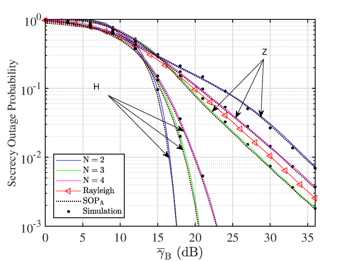
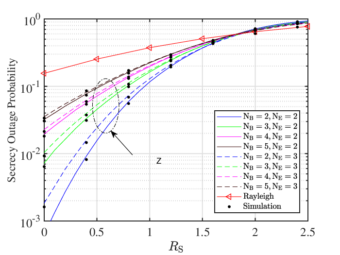
Fig. 5 presents the evolution of the SOP as a function of $R_{S}$, considering the following channel settings: $\overline{\gamma}_{\mathrm{E}}=1$ dB, $\overline{\gamma}_{\mathrm{B}}=8$ dB, $K_{\mathrm{dB}}^{\mathrm{B}}=K_{\mathrm{dB}}^{\mathrm{E}}=20$ dB, and $\left\{\alpha_{\mathrm{B}},\alpha_{\mathrm{E}}\right\}$$=$$\left\{0.2,0.3\right\}$. Herein, we analyze the effect of having a different number of dominant specular rays at both Bob and Eve over the secrecy performance. We consider the cases $\mathrm{N}_{\mathrm{E}}=\left\{2,3\right\}$ and $\mathrm{N}_{\mathrm{B}}=\left\{2,3,4,5\right\}$, and for the sake of comparison, we also include the case $\mathrm{N}_{\mathrm{B}}=\mathrm{N}_{\mathrm{E}}$. Once again we see that having a larger number of multipath waves at the legitimate receiver in this unbalanced scenario effectively increases channel variability, which causes the SOP obtained when transmitting at a rate $R_{\mathrm{S}}$ to be increased with $\mathrm{N}_{\mathrm{B}}$. We also see that for a fixed $\mathrm{N}_{\mathrm{B}}$, increasing the number of rays on the eavesdropper’s channel is also detrimental for the SOP. This can be understood by recalling that in the presence of a single dominant specular component for each link and a strong LOS condition, the set-up almost reduces to the AWGN case, for which the SOP is zero as $\overline{\gamma}_{\mathrm{B}}>\overline{\gamma}_{\mathrm{E}}$. Hence, having a reduced number of rays and a dominant component much larger than the remaining specular waves turn out being beneficial for physical layer security.

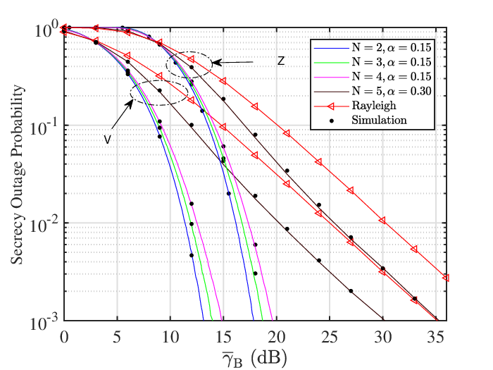
Next, Fig. 6 illustrates the SOP vs. $\overline{\gamma}_{\mathrm{B}}$ for different numbers of rays $\mathrm{N}_{\mathrm{B}}=\mathrm{N}_{\mathrm{E}}=\mathrm{N}$ with $\overline{\gamma}_{\mathrm{E}}=1$ dB, $K_{\mathrm{dB}}^{\mathrm{B}}=25$ dB, and $K_{\mathrm{dB}}^{\mathrm{E}}=0$ dB. Moreover, we set: $R_{\mathrm{S}}=\left\{1,2.5\right\}$ with $\alpha=\alpha_{\mathrm{B}},=\alpha_{\mathrm{E}}=0.15$ and $\alpha=\alpha_{\mathrm{B}},=\alpha_{\mathrm{E}}=0.30$ for $\mathrm{N}=2,\dots 4$, and $\mathrm{N}=5$, respectively. From the figure can be observed that both the relative amplitudes and the number of the dominant waves play a pivotal role on the secrecy performance. For instance, we see that the decay of the SOP is rather abrupt for $\alpha=0.15$ and $\mathrm{N}=1,\dots,4$ regardless of the choice of $R_{\mathrm{S}}=\left\{1,2.5\right\}$. However, when both the number of rays and the relative amplitudes of the rays are slightly increased (say $\alpha=0.3$ and $\mathrm{N}=5$), then the SOP is dramatically impaired and the decay is now similar to the Rayleigh case. This is in coherence with the observations made in [12] in the limit case of the absence of diffuse scattering, as $\alpha\left(\mathrm{N}_{\mathrm{B}}-1\right)<1$.

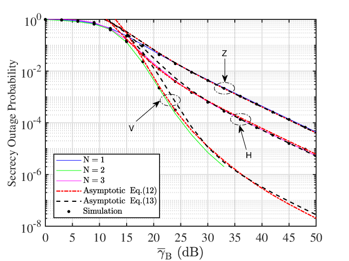
Finally, in Fig. 7, we plot the SOP vs. $\overline{\gamma}_{\mathrm{B}}$ and the two asymptotic results (12), (13), respectively. In all the cases, we employ equal numbers of rays at both $\mathrm{B}$ and $\mathrm{E}$, i.e., $\mathrm{N}=\mathrm{N}_{\mathrm{B}}=\mathrm{N}_{\mathrm{E}}$, $R_{\mathrm{S}}=1$ bps/Hz, $\Omega_{\mathrm{B}}=\Omega_{\mathrm{E}}=1$, and $\overline{\gamma}_{\mathrm{E}}=8$ dB. Also, yet without loss of generality, we assume the following cases: Case $\mathrm{I}$ $(\mathrm{N}=1)$: Balanced amplitudes, $V_{1,\mathrm{B}}=V_{1,\mathrm{E}}=1$, and $K_{\mathrm{dB}}^{\mathrm{B}}=K_{\mathrm{dB}}^{\mathrm{E}}=10$ dB; Case $\mathrm{II}$ $(\mathrm{N}=2)$: Unbalanced amplitudes, $V_{2,i}=\alpha_{2,i}V_{1,i}$ with $V_{1,i}=1$ for $i$ $\in\left\{\mathrm{B},\mathrm{E}\right\}$, $\alpha_{2,\mathrm{B}}=0.2$, $\alpha_{2,\mathrm{E}}=0.9$, and $K_{\mathrm{dB}}^{\mathrm{B}}=K_{\mathrm{dB}}^{\mathrm{E}}=15$ dB; Case $\mathrm{III}$ $(\mathrm{N}=3)$: Unbalanced amplitudes, $V_{n,i}=\alpha_{n,i}V_{1,i}$ with $V_{1,i}=1$ for $i$ $\in\left\{\mathrm{B},\mathrm{E}\right\}$, $\alpha_{n,i}=\alpha_{\mathrm{B}}=\alpha_{\mathrm{E}}=0.3$ for $n=2,3.$, and $K_{\mathrm{dB}}^{\mathrm{B}}=K_{\mathrm{dB}}^{\mathrm{E}}=10$ dB. Here, our primary aim is to analyze the secrecy diversity order of the main links in the proposed scenarios. Firstly, based on the asymptotic expressions (i.e., (12), and  (13)), we see that the exponents for the $\overline{\gamma}_{\mathrm{B}}$ terms depend on one of the summation indexes (i.e., $(k_{\mathrm{B}}+1)$). This suggests that each of these terms contributes in different ways to the decay of the SOP, which explains that the slope of the SOP is different depending on the range of values of $\overline{\gamma}_{\mathrm{B}}$. As the SNR is increased, it is only the first term of the series which contributes to the SOP, revealing a diversity order of one (vide all cases in Fig. 7). However, we can see that such diversity order is not useful for Case $\mathrm{II}$, which justifies the need of the more accurate asymptotic expressions here provided, compared to those only relying on $\mathrm{G}_{d}$ expression. Also, we can observe that the asymptotic analytical in (12) is tighter than the asymptotic one given in (13).

We investigated how the explicit consideration of the incident waves arriving at the receiver ends may impact physical layer security performance in the context of wireless fading channels. The analytical results here presented complement and generalize those previously reported in the literature, and support the need of using ray-based fading models in those situations on which a reduced number of multipath waves are considered. The main takeaways of our work can be summarized as: $(i)$ abundant dominant specular rays impair the SOP, so scenarios with a reduced number of rays arriving at both Bob and Eve are beneficial whenever $\overline{\gamma}_{B}>\overline{\gamma}_{E}$; $(ii)$ balanced amplitudes for the eavesdropper’s link and unbalanced amplitudes for the desired link are the most favorable case from a PLS perspective; $(iii)$ a significant increase on the power of Bob’s dominant specular components with respect to the power of Eve’s dominant specular components (i.e., $K_{\mathrm{B}}>>K_{\mathrm{E}}$), in the case of balanced amplitudes, is a worst case scenario for secrecy performance.

References

- [1] D. Liu, W. Hong, T. S. Rappaport, C. Luxey and W. Hong, “What will 5G Antennas and Propagation Be?,” IEEE Trans. Antennas Propag., vol. 65, no. 12, pp. 6205–6212, Dec. 2017.
- [2] M. K. Samimi, G. R. MacCartney, S. Sun, and T. S. Rappaport, “28 GHz Millimeter-Wave Ultrawideband Small-Scale Fading Models in Wireless Channels,” in 2016 IEEE 83rd Veh. Technol. Conf. (VTC-Spring), May 2016.
- [3] G. Taricco, “On the Convergence of Multipath Fading Channel Gains to the Rayleigh Distribution,” IEEE Wireless Commun. Lett. vol. 4, no. 5, pp. 549–552, Oct. 2015.
- [4] G. D. Durgin, T. S. Rappaport, and D. A. de Wolf, “New Analytical Models and Probability Density Functions for Fading in Wireless Communications,” IEEE Trans. Commun., vol. 50, no. 6, pp. 1005–1015, Jun. 2002.
- [5] J. M. Romero-Jerez, F. J. López-Martínez, J. F. Paris, and A. J. Goldsmith, “The Fluctuating Two-Ray Fading Model: Statistical Characterization and Performance Analysis,” IEEE Trans. Wireless Commun., vol. 16, no. 7, pp. 4420–4432, Jul. 2017.
- [6] J. M. Romero-Jerez, F. J. Loṕez-Martínez, J. F. Paris, and A. Goldsmith, “The Fluctuating Two-Ray Fading Model for mmWave Communications,” in Proc. IEEE Globecom Workshops (GC Wkshps), Washington, DC, USA, Dec. 2016, pp. 1–6.
- [7] M. Bloch, J. Barros, M. R. D. Rodrigues, and S. W. Mclaughlin, “Wireless Information-Theoretic Security,” IEEE Tran. Inf. Theory, vol. 54, no. 6, pp. 2515–2534, Jun. 2008.
- [8] J. D. Vega Sánchez, L. Urquiza-Aguiar, and M. C. P. Paredes, “Physical Layer Security for 5G Wireless Networks: A Comprehensive Survey,” in 2019 IEEE 3rd Cyber Security in Networking Conference (CSNet), to be published, 2019.
- [9] D. P. Moya Osorio, J. D. Vega Sánchez, and H. Alves, “Physical Layer Security for 5G and beyond,” in 5G REF: The Essential 5G Reference Online, John Wiley & Sons, 2019, ch. 1, pp. 1–19.
- [10] W. Zeng, J. Zhang, S. Chen, K. P. Peppas, and B. Ai, “Physical Layer Security Over Fluctuating Two-Ray Fading Channels,” IEEE Trans. Veh. Technol., vol. 67, no. 9, pp. 8949–8953, Sep. 2018.
- [11] L. Wang, N. Yang, M. Elkashlan, P. L. Yeoh, and J. Yuan, “Physical Layer Security of Maximal Ratio Combining in Two-Wave With Diffuse Power Fading Channels,” IEEE Trans. Inf. Forensics Security, vol. 9, no. 2, pp. 247–258, Feb. 2014.
- [12] P. Ramírez-Espinosa, R. J. Sánchez-Alarcón ,and F. J. López-Martínez “On the Beneficial Role of a Finite Number of Scatterers for Wireless Physical Layer Security,” Oct. 2019, arXiv:1910.09856. [Online].
- [13] Y. J. Chun, “A Generalized Fading Model with Multiple Specular Components,” Oct. 2018, arXiv:1810.05258. [Online].
- [14] J.M. Romero-Jerez, F.J. Lopez-Martinez, J.P. Pena-Martin, and A. Abdi, “Stochastic Fading Channel Models with Multiple Dominant Specular Components for 5G and Beyond,” May 2019, arXiv:1905.03567 [Online].
- [15] Abramowitz, M. and Stegun, I. A., “Handbook of Mathematical Functions, US Dept. Of Commerce, National Bureau Of Standards, Washington DC, 1972.
- [16] G. D. Durgin, “Theory of Stochastic Local Area Channel Modeling for Wireless Communications,” PhD diss., Virginia Tech, 2000.
- [17] C. Chen and A. Abdi, “Bit error rate in multipath wireless channels with several specular paths,” Electronics Letters vol. 47, no. 18, pp. 1046 -1048, 1 September 2011.
- [18] T. Bai and R. W. Heath Jr., “Coverage and Rate Analysis for Millimeter-wave Cellular Networks,” IEEE Trans. Wireless Commun., vol. 14, no. 2, pp. 1100–1114, Feb. 2015.
- [19] A. D. Wyner, “The wiretap channel,” Bell Syst. Tech. J., vol. 54, no. 8, pp. 1355–1387, Oct. 1975.
- [20] I. S. Gradshteyn and I. M. Ryzhik, Table of Integrals, Series and Products, 7th ed., San Diego, CA, USA: Academic Press, 2007.