Precision and consistency of astrocombs2020Precision and consistency of astrocombs–17
Abstract
Astrocombs are ideal spectrograph calibrators whose limiting precision can be derived using a second, independent, astrocomb system. We therefore analyse data from two astrocombs (one and one ) used simultaneously on the HARPS spectrograph at the European Southern Observatory. The first aim of this paper is to quantify the wavelength repeatability achieved by a particular astrocomb. The second aim is to measure wavelength calibration consistency between independent astrocombs, that is to place limits or measure any possible zero-point offsets. We present three main findings, each with important implications for exoplanet detection, varying fundamental constant and redshift drift measurements. Firstly, wavelength calibration procedures are important: using multiple segmented polynomials within one echelle order results in significantly better wavelength calibration compared to using a single higher-order polynomial. Segmented polynomials should be used in all applications aimed at precise spectral line position measurements. Secondly, we found that changing astrocombs causes significant zero-point offsets ( in our raw data) which were removed. Thirdly, astrocombs achieve a precision of in a single exposure ( above the measured photon-limited precision) and when time-averaged over a few hours, confirming previous results. Astrocombs therefore provide the technological requirements necessary for detecting Earth-Sun analogues, measuring variations of fundamental constants and the redshift drift.
Keywords:
instrumentation: spectrographs – instrumentation: detectors – techniques: spectroscopic – techniques: radial velocities – cosmology: cosmological parameters – cosmology: dark energy1 Introduction
Measuring spectroscopic velocity shifts () in high resolution astronomical spectra is a powerful and widely used tool in a range of astronomical disciplines. It is used to detect planets outside of the Solar System (Mayor & Queloz 1995; Anglada-Escudé et al. 2016), look for variation in the values of fundamental constants (e.g. the fine strucure constant, , Dzuba et al. 1999; Webb et al. 1999; Webb et al. 2011; King et al. 2012, and others). It is also the method proposed to measure the expansion of the Universe in “real time” and in a model-independent way (also known as the Sandage test or the “redshift drift” measurement, Sandage 1962; Loeb 1998; Liske et al. 2008) and to map the gravitational potential of the Galaxy (Ravi et al. 2019; Leão et al. 2019). These science goals are important drivers for all 30-meter class telescopes planned for the 2020s, i.e. the Extremely Large Telescope (Tamai et al. 2018, ELT,), the Thirty Meter Telescope (Simard et al. 2016, TMT,), and the Giant Magellan Telescope (Fanson et al. 2018, GMT,). This is why all will be equipped with a high resolution optical spectrograph.
The success of these projects relies not only on increasing the light gathering capability of telescopes, but also on the instrument stability, and the precision and accuracy with which velocity shifts in astronomical spectra can be measured. In this context, precision is the repeatability of subsequent wavelength measurements to each other and accuracy is the closeness of a measured wavelength to its true value. The most demanding of the four aforementioned projects – the redshift drift measurement – requires velocity shifts be measured with a precision better than 3 part in 100 billion over spectral ranges of several hundred nanometers and a period longer than ten years. This corresponds to , or equivalently, 1 centimeter per second (). The best way to ensure long term precision is to ensure that the measured wavelengths are also accurate. Instruments intended to perform these experiments are therefore designed to have wavelength calibration precision around and accuracy of order 1 metre per second () over a period of a decade (Liske 2014; Marconi et al. 2016, e.g.). The success of these projects thus critically relies on the precision and accuracy of the wavelength calibration reaching these levels.
The currently most commonly used method of wavelength calibration in high resolution spectrographs uses hollow cathode lamp, most commonly Thorium (Th) and Uranium (U) lamps. The hollow cathode lamp calibration suffers from several major drawbacks limiting its precision to a few tens of over a period of one year and average accuracy of approximately in the same period (Lovis et al. 2006), thus falling short of the previously stated goals. It is now generally accepted that laser frequency comb system (Udem et al. 2002; Hänsch 2006, LFC,) can achieve substantially better results to push the precision and accuracy of wavelength calibration to the level and ensure the feasibility of the scientific projects mentioned above. For a recent review about laser frequency comb spectroscopy, see Picqué & Hänsch 2019.
Laser frequency combs offer significant advantages over arc lamps: (i) they produce thousands of unblended emission lines of uniform intensity and equidistant in frequency; and (ii) the frequencies of LFC lines are a priori known with accuracy of the atomic clock to which the system is coupled (typically or ). Murphy et al. 2007 discusses the advantages of LFCs in more detail. LFCs do not suffer from lamp aging in the same way as hollow cathode lamps, but their components (e.g. the photonic crystal fibre, PCF) degrade.
The European Southern Observatory (ESO) formed a consortium to develop and install an astronomical LFC (also known as an “astrocomb”) on the HARPS instrument in 2008. The development saw several test campaigns after which the astrocomb was permanently installed on HARPS in May 2015. This astrocomb has already demonstrated short-term precision at the photon noise level, or (Wilken et al. 2012). Similar short-term precision using astrocombs has also been demonstrated on several other high-resolution spectrographs (Ycas et al. 2012; Phillips et al. 2012; Doerr et al. 2012; Glenday et al. 2015; Brucalassi et al. 2016; McCracken et al. 2017, e.g.). All these previous studies referenced the astrocomb to itself, so any possible systematic effects arising in the astrocomb system itself may go undetected.
Definitive proof of astrocomb performance can only come from its comparison to another calibration source of the same (or higher) precision. This is why, in a campaign that took place in April 2015, two independent astrocomb systems were installed on HARPS: one constructed for the HARPS instrument itself and the other constructed for the FOCES instrument (Pfeiffer et al. 1992). The experiment had two goals. The first one was to understand whether the precision of a single astrocomb is confirmed by an independent system, and the second one was to assess zero-point offsets in the wavelength calibration introduced by switching between the two astrocombs.
Probst et al. 2020 analyses the same dataset, but with a focus on describing the experimental setup, astrocomb hardware and its optimisation during the campaign before the astrocomb’s deployment in May 2015. This paper, on the other hand, focuses on data analysis techniques and advanced algorithms that will provide wavelength calibration precision required by the ELT projects discussed above.
The paper is divided as follows: in section 2 we briefly describe the experimental setup – the spectrograph and the two astrocombs. section 3 describes the dataset and general properties of the spectra. section 4 gives details on our automatic algorithm to detect astrocomb lines and obtaining their centres and wavelengths. Wavelength calibration is discussed in section 5, where we describe how we deal with instrumental effects that impact significantly on wavelength calibration precision and accuracy, e.g. defects associated with the CCD manufacturing process. In the same section, we describe our findings on the optimal wavelength calibration model for HARPS spectra. We present our findings on precision and consistency in section 6, where we also consider and model the contribution of flux dependent velocity shifts. Finally, our results are presented in section 7 and discussed in section 8.
2 Experimental setup
2.1 The HARPS instrument
The High Accuracy Radial velocity Planet Searcher (Mayor et al. 2003, HARPS,) was built for extreme stability and precision and is one of the most stable astronomical spectrographs in existence. HARPS is a fibre fed, high-resolution (), R4 grism cross-dispersed echelle spectrograph installed on the 3.6m telescope at ESO’s La Silla Observatory and the first instrument to be equipped with an astrocomb for regular operations (Probst et al. 2016). The light of the two input fibres is dispersed into 72 echelle orders on the detector, simultaneously covering the wavelength range between 378 and 691 nm. The spectrograph is enclosed in a thermal and pressure controlled vacuum vessel, with long-term temperature variations at the 0.01K level and operating pressure below .
Several thermal and mechanical effects can slightly shift the positions of the spectrum on the detector with time, an unavoidable effect that is eliminated through simultaneous referencing: drifts in the science fibre are tracked by simultaneously observing a spectrum rich in velocity information content (e.g. ThAr, an astrocomb, or a Fabry-Pérot etalon) in the secondary fibre (Baranne et al. 1996). Each fibre has a static double scrambler. A servo controller (“secondary guiding”) ensures that the object image is always centered in the object fibre. In order to ensure light entrance stability and proper mode mixing in the fibres, a dynamical fibre scrambler that shakes the fibres was added to the setup, adding a temporal scrambling of light (Probst et al. 2020).
2.1.1 The detector
The HARPS detector is a mosaic of two EEV2k4 CCDs (red and blue). Each CCD is constructed by stitching together pix2 segments: eight in the dispersion () direction and two in the cross-dispersion () direction. CCD pixels have a nominal size of but errors in the segment stitching process results in deviations from the nominal pixel size at segment boundaries, i.e. every 512 pixels in the direction and every 1024 in the direction.
The HARPS detector was the first one shown to suffer from the effect of imperfect CCD stitching (Wilken et al. 2010). Dumusque et al. 2015 showed that lines which cross segment boundaries produce spurious velocity shifts as high as a few with a period of one year in HARPS observations. Proper mitigation of this effect is therefore important for exoplanet detection and also for fundamental constant and redshift drift measurements. The way this has been done previously is to shift the measured positions of calibration lines (in pixel space) by the measured size of pixel size anomalies during wavelength calibration. Pixel size anomalies were measured by Bauer et al. 2015 using Fabry-Pérot etalon exposures and by Coffinet et al. 2019 using flat-field exposures. We perform a similar measurement using astrocombs exposures in section 5.1. Therefore, in section 5.2, we examine the effectiveness of different calibration methods in removing the effect of pixel size anomalies.
2.2 The astrocombs
Astrocombs are laser frequency comb systems built specifically to wavelength calibrate astronomical spectrographs (Steinmetz et al. 2008). They produce thousands of emission lines (or modes) of uniform intensity with precisely known frequencies. The nominal frequency of each mode is given by the “LFC equation”:
| (1) |
where and are the “offset” and the “repetition” frequencies, and is the mode number (a large positive integer). Both and are radio-frequencies referenced to an atomic clock and known with precision of over the timescale of several hours (Probst et al. 2020). The frequency, and the wavelength, of each line can therefore be determined with the same precision.
The HARPS astrocomb development saw several test campaigns between January 2009 and April 2015. One of the goals of the April 2015 campaign was to characterise the performance of the HARPS astrocomb against a completely independent second one. The second astrocomb, built for the FOCES instrument (Pfeiffer et al. 1992), was loaned from the Wendelstein Observatory (operated by Ludwig-Maximillians-Universität, LMU) for this purpose. The HARPS astrocomb has an line separation. Since the HARPS spectral resolution is around in the middle of its spectral range, astrocomb lines are kept well apart with virtually no residual overlap. We will refer to this astrocomb as “LFC1” in further text. To accommodate the lower resolution of the FOCES instrument (), the FOCES astrocomb was designed with a wider line separation of . We will refer to this astrocomb as “LFC2” in further text. Wavelength coverage of the two astrocombs differs slightly due to different requirements for the HARPS and FOCES instruments. Relevant information about the two astrocombs are tabulated in Table 1. See Probst et al. 2020 for a more comprehensive description of the astrocomb design and the setup during the April 2015 campaign.
3 Data
3.1 The dataset
We use a time series of spectra of the two astrocombs described above for our analysis. The series consists of a total of 194 exposures. Each exposure was 30 seconds long with a read-out time of 22 seconds. The entire duration of the series is approximately six hours, with a two hour gap between the end of exposure 94 and the beginning of exposure 95. In the first 94 exposures, fibre B (the object fibre) was illuminated with LFC2, after which the astrocomb was changed and 100 exposures of LFC1 were taken in the same fibre. We therefore divide the dataset into two samples, depending on which astrocomb illuminated fibre B. We will refer to the “LFC2 sample” for exposures 1–94 and to the “LFC1 sample” for exposures 95–194. Meanwhile, LFC2 was used as a simultaneous reference in fibre A (simultaneous fibre), keeping track of spectrograph drifts throughout the whole series, for a total of 194 exposures in fibre A. Figure 1 gives a schematic of the series of exposures we use in our analysis.
| LFC1 | LFC2 | |
|---|---|---|
| Native | ||
| Mode filtering | 72 | 100 |
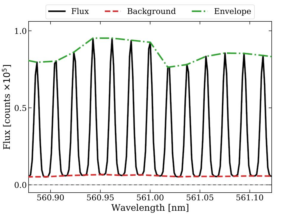
We choose to work on ‘e2ds’ files – unmerged 1D spectra extracted from raw images by the HARPS pipeline (version v3.8) using optimal extraction after Horne (1986). Each e2ds file consists of 72 (71) echelle orders covering 4096 pixels of an exposure in fibre A (B). The detector covers echelle orders 89 to 161, with the exception of order 115 for fibre A and orders 115 and 116 for fibre B, which fall in between the two detector CCDs. A fraction of the LFC1 spectrum showing individual lines around in echelle order 109 is plotted in Figure 2.
We limit our analysis to echelle orders 89–130, where the fluxes of the two astrocombs are sufficiently high and comparable – as evidenced by the total number of counts detected in each echelle order (see Figure 3). This covers wavelengths between and , or 70% of the total HARPS wavelength range.
A quantity that is directly relevant for exoplanet detection studies, but not for varying constant or redshift drift measurements, is the uncertainty on the mean velocity shift that can be determined in a spectrum. This measure of uncertainty is determined by the photon noise and other detailed spectral attributes – see Bouchy et al. 2001 and Murphy et al. 2007 for details. We will refer to this quantity as “photon-limited velocity precision”. We calculate the photon-limited velocity precision of individual exposures in our dataset across orders 89 – 130. We find that the average photon-limited velocity precision of a single exposure in the LFC1 sample is () in fibre A (B); and in the LFC2 sample is () in fibre A (B). The reduced photon-limited velocity precision in fibre B is attributable to lower flux compared to fibre A for both samples.
3.2 Spectral background
The spectra obtained using both astrocombs exhibit a strong background component (the red line in Figure 2 illustrates the background light in the LFC1 spectrum). This background originates mostly from amplified spontaneous emission (ASE) in the high-power Yb-fibre amplifier (Probst et al. 2013; Probst et al. 2020) and, to a lesser extent, from scattered light (Rodler & Lo Curto 2019, measured to be at in the HARPS spectrograph). The ASE from the high-power amplifier is further amplified by non-linear processes in the photonic crystal fibre, located just after it in the optical path. We refer the reader to Probst et al. 2020 for more technical details on the origin of the background.
The background is highly modulated, approximately tracing the variations in intensity of astrocomb lines. We characterize the contribution of the background to the total detected flux in terms of the background-to-envelope ratio (B2E). The background here refers to a function connecting the local minima in the spectrum. This is a piece-wise linear function of pixel number, :
| (2) |
where is flux (in units counts) and and are locations of adjecent minima in the spectrum. The envelope is the analogous quantity except maxima instead of minima are fitted. Both are illustrated in Figure 2.
Our analysis shows that B2E increases linearly with decreasing wavelength, with values between 2% and 16% in a typical exposure in both astrocombs. The background is therefore non-negligible. To minimise any impact on estimating astrocomb line centres, we subtract the background from the total flux, propagating the errors to correctly modify the spectral variance array:
| (3) |
where we have assumed that the flux and the background are Poissonian and the detector noise (i.e. dark-current, read-out-noise) is negligible.
4 Astrocomb lines
4.1 Line detection
Our line detection algorithm automatically detects all astrocomb lines in the exposure. The algorithm relies on locating minima between individual lines as their natural limits. We found this practice to be preferred over using maxima, as the latter caused issues with falsely detected and skipped lines when using an automated detection routine. Line detection is done in three steps. In the first step, we smooth the recorded spectrum of an echelle order with a Wiener filter with a 3 (5) pixel wide window for LFC1 (LFC2). The smoothed spectrum makes identifying minima easier in the following step. In the second step, we identify local minima as points where the first derivative (with respect to the pixel number) switches sign, and the second derivative is larger than zero. This step sometimes falsely detects minima in the data, especially when the signal-to-noise ratio (S/N) is low. We therefore reject falsely detected minima in the third and final step, using the following two assumptions: (i) the distance between minima must not significantly deviate from typical distance between astrocomb lines; and (ii) the distance between minima within the echelle order increases approximately linearly with increasing wavelength.
We use the first assumption to remove minima closer together than 90% of the typical distance between lines in the same echelle order, where the latter is equal to period of the strongest peak in the periodogram of the order. Depending on the astrocomb and the echelle order, this number is between 11 and 20 pixels, with LFC2 always having larger values due to larger mode separation. The second assumption follows directly from Equation (1): the separation of consecutive lines in wavelength space approximately follows , where is the wavelength of the astrocomb mode. This means that the distance between lines increases approximately linearly in pixel space within a single echelle order. We therefore remove outliers to the linear function best describing , where is the distance between adjacent lines.
Our automatic line detection algorithm detects and in each LFC1 and LFC2 exposure (where the background was subtracted), respectively. Across the entire dataset, we detect lines in fibre A and lines in fibre B, with a total lines. The average signal-to-noise ratio (S/N) of lines is approximately 165, with differences between LFC1 versus LFC2 and fibre A versus fibre B.
4.2 Profile fitting
In this analysis we assume that each astrocomb line can be well-represented by a single Gaussian profile. Visual examination of the data suggests that the approximation is generally reasonable although asymmetries are seen depending on position on the CCD. We will explore different ways of modelling astrocomb profiles in a forthcoming paper.
We use a Levenberg-Marquardt algorithm11 1 leastsq routine from scipy.optimize to derive best-fit Gaussian parameters for each line. Since the data are high signal-to-noise, and since slight non-linearities in the model function exist across individual spectral pixels, the model-fitting procedure avoids simply computing the Gaussian value at the centre of each pixel but instead performs an integration of the flux falling within each pixel. The expected number of counts in each pixel (with and its left and right boundaries) is given by:
| (4) |
Here is the error function, and , , and are the amplitude, the mean and the standard deviation of the Gaussian, respectively. The algorithm provides a line-centre uncertainty estimate for each line. The mean line-centre uncertainty across all detected lines is 3 milli-pixel (mpix). An example fit for a single LFC1 line is shown in Figure 4.
Ultimately, the Gaussian approximation above is incorrect. This can be seen by eye from the asymmetric shape of astrocomb lines and is evident from the high values of reduced values (, with the number of degrees of freedom) we get for the Gaussian line fits. The distribution derived from Gaussian fitting, shown in Figure 5, peaks at and has a mean across the detector, indicating an overall poor fit to the data. Large values for Gaussian fits are concentrated in two regions: in the red half () of echelle orders 89–98 and the middle part of orders 125–130 (). The values do not correlate with any of the fit parameters or their errors. The same pattern is seen independently for both astrocombs and in both fibres. This suggests that the pattern must be due to variation in the line-spread function profile across the detector.
Whilst a Gaussian is clearly not the correct line shape, we show later that the Gaussian approximation nevertheless performs well in term of repeatability such that radial velocity studies are relatively unaffected by the correlated patterns seen in Figure 5. We note however that this issue will be important for other types of studies such as varying constants and redshift drift. We will later derive a model of the line-spread function – assuming it will also give us a more accurate estimation of the line centre (Milaković et al. prep).

4.3 Mode identification
Astrocomb wavelength calibration requires another wavelength calibration source to establish the absolute scale by identifying a single line in each echelle order, after which the frequencies of all lines are known by counting. This is not a critical aspect as long as the error in the absolute calibration source is much smaller than half of the separation between astrocomb lines. The local accuracy of ThAr wavelength calibration, the HARPS standard, is between and or to at , (respectively). This is well below the line separation of either astrocomb (Table 1). We therefore use the ThAr wavelength calibration to identify a single astrocomb mode per echelle order in the following way. The mode number, , is the nearest integer to the number:
| (5) |
where is frequency of the astrocomb line determined from the ThAr wavelength calibration, and are the astrocomb offset and repetition frequencies, respectively. These frequencies are recorded by the astrocomb system22 2 The experimental nature of the April 2015 campaign meant of both astrocombs was changed multiple times. We discover an un-noted shift in LFC1 of whilst analysing the daset. More details can be found in Appendix A.. We always use the same ThAr coefficients to determine the mode number of the line closest to pixel 2048, where the ThAr calibration is expected to be the most accurate.
The wavelength and the corresponding uncertainty of each line are calculated from equations:
| (6) |
and
| (7) |
with the speed of light and is the frequency uncertainty for each line. Empirically, . Uncertainties at this level are generally orders of magnitude below spectral line uncertainties in astronomical targets such as quasars.
5 Wavelength calibration
Spectrograph wavelength calibration relates the measured positions of a set of calibration lines on the detector with their known laboratory wavelengths in a way that assigns a wavelength to each position on the detector. The most common approach in optical echelle spectroscopy is to fit a polynomial to a set of calibration lines in each extracted echelle order. The large number of astrocomb lines and the exquisite accuracy with which their wavelengths are known allow us to look for a more realistic model, e.g. by increasing the polynomial order (Wilken et al. 2010, see e.g.). In this Section we examine a range of polynomial orders in an attempt to identify an optimal number of degrees of freedom.
Furthermore, it is generally assumed that all pixels have the same physical size, so that the physical distance between calibration lines on the detector can be expressed in pixel distance. This assumption has been proven invalid by the discovery of the HARPS detector pixel size anomalies (see section 2.1.1). Distortions of the HARPS wavelength scale caused by the pixel size anomalies can be removed using one of the following two approaches: (i) global polynomial: producing a wavelength calibration spanning the entire echelle order in which the anomalies have been accounted for (see section 5.1), and (ii) segmented polynomials: producing a separate wavelength calibration for each 512-pixel CCD segment that an echelle order crosses. Coffinet et al. 2019 take the former approach, whereas Wilken et al. 2010 and Molaro et al. 2013 take the latter. In this analysis we use the Akaike information criterion (Akaike 1974, AIC,), corrected for the finite sample size (Sugiura 1978, AICc,), in order to asses which of these two approaches provides the best results (section 5.2).
In what follows, we make extensive use of Weighted Orthogonal Distance Regression33 3 Python package scipy.odr, based on ODRPACK (Boggs et al. 1992), an algorithm which allows us to account for both the positional and wavelength uncertainty of astrocomb lines in polynomial fitting.
5.1 Measuring HARPS detector pixel size anomalies
We derive our pixel size anomaly measurements from distortions of the HARPS wavelength scale revealed by the astrocomb lines. Astrocomb wavelength coverage limits us to only three out of four -blocks: two blocks of the red CCD (blocks 1 and 2 in further text) and a single block of the blue CCD (block 3 in further text).
Pixel size anomalies are measured for each block individually using the wavelength calibration residuals in the following way:
- 1.
For a given detector -block, we consider only those echelle orders which fall onto the block. It seems likely that distortions in the direction are common to all orders that fall within the same 1024-pixel high CCD block in the direction. If this is not the case, the effect would be to increase the scatter in the -direction within each block (the shaded region) in Figure 6;
- 2.
We fit a global eighth order polynomial to pixel-wavelength pairs of astrocomb lines separately in each echelle order and each exposure. We calculate the residuals to the true line wavelengths (i.e. Equation (1)) and express them in ;
- 3.
We bin the residuals in 64 bins along the axis (i.e. giving 8 points per 512 pixel-wide segment), excluding lines closer to segment borders than 10 pixels and those with residuals larger than ;
- 4.
We fit a third order polynomial to the binned residuals. A typical error on each binned residual is of order due to the large number of points in each bin ().
- 5.
The discontinuity is given by the difference between the polynomials in two adjacent segments at their boundary (in units ):
(8) Here, and are the polynomials in two adjacent segments and is the position of the discontinuity (in pixels, multiple of 512);
- 6.
We convert the discontinuity into the pixel size anomaly by dividing it by the size of the HARPS pixel in velocity units in the middle of the HARPS wavelength range: .
This is illustrated in Figure 6 using data from fibre A. Measurements from fibre B (not illustrated) were found to be consistent with those from fibre A; there are a total of 21 pixel size anomaly measurements from each fibre. Differences between corresponding pixel size anomaly pairs were measured for all 21 pairs. The unweighted mean of those numbers is mpix, corresponding to .
Although the two fibres produced completely consistent results, the results from fibre A seemed better than from fibre B, in that the scatter in the fibre B residuals (Figure 6) were more pronounced. We did not attempt to explore the reason for this and simply used fibre A to make the corrections. These are tabulated in Table 2 and used to adjust the positions of individual astrocomb lines. The corrected position of one line within one echelle order, in pixels, is given by:
| (9) |
where and are the corrected and the fitted line positions of the same line and is the size of a pixel size anomaly located at the pixel.

Our measurements are in very good agreement with previous, independent, results. The average agreement with the results of Bauer et al. 2015 is mpix (). Similarly, agreement with the results of Coffinet et al. 2019 is mpix (). This corresponds an agreement between the two measurements at the level on the detector. Unlike the flat-field method of Coffinet et al. 2019, we are not sensitive to the sizes of individual pixels at segment borders but only to the sum of their sizes. Our astrocomb method is, however, complementary to theirs and serves as a consistency check. Furthermore, it demonstrates the usefulness of astrocombs for detector characterization necessary to obtain robust scientific results.
| CCD | Red | Blue | ||
|---|---|---|---|---|
| Orders | 89–99 | 100–114 | 116–134 | 135–161 |
| Block | 1 | 2 | 3 | 4 |
| 423k | 698k | 754k | 0 | |
| Pixel | Pixel size anomaly [mpix] | |||
| 512 | 34.97 | 53.62 | 32.27 | – |
| 1024 | 7.67 | -23.79 | 13.79 | – |
| 1536 | 39.12 | 30.88 | 19.72 | – |
| 2048 | 0.14 | 30.56 | 13.06 | – |
| 2560 | 11.77 | 9.82 | 18.40 | – |
| 3072 | 48.28 | 41.86 | 61.89 | – |
| 3584 | 21.78 | 3.18 | 7.07 | – |
5.2 Choosing a wavelength calibration model
We return to our aim of determining the model the optimal residuals number of degrees of freedom. We do this using the AIC corrected for small sample sizes (Sugiura 1978, AICc,) and choose the model providing the smallest residuals using the smallest number of free parameters possible. The AICc is calculated as:
| (10) |
where is the number of free parameters and is the number of data points used in the fit. Theoretically, the model with the lowest AICc value is preferred.
We consider a total of 29 wavelength calibration models, grouped into two groups mentioned beforehand: the segmented and the global polynomial models. The segmented polynomial models range between and order, whereas the global polynomials range between and order. The former have free parameters and the latter have free parameters, with the highest order polynomial in the model.
For segmented polynomial models, we divide the echelle order into eight 512-pixel wide segments and fit a polynomial in each segment individually. We do not impose conditions on the continuity or smoothness of the polynomials at segment boundaries and leave the parameters in each segment independent, resulting in a discontinuous wavelength calibration model. In the case of global polynomial models, we first adjust the positions of individual lines to account for the CCD stitching pattern using Equation (9), after which we fit a single polynomial to all astrocomb lines in the echelle order.
We calculate AICc values for all 29 models, for each of the 43 echelle orders, for each of the 194 exposures, and for each fibre. There are therefore 66736 AICc values for each segmented polynomial model (i.e. for each parabolic, cubic, quadratic, quintic, etc.), and 8342 values for each global polynomial model, for each fibre. Considering the large number of individual fits, we look at AICc in a statistical sense when comparing models: the best model is the one with the lowest mean AICc, where that mean is averaged over all echelle orders and all exposures. The mean AICc for all 29 models is plotted in Figure 7, separately for the segmented (top panel) and global polynomials (bottom panel).
The segmented polynomial model with the lowest mean AICc is a seventh order polynomial (), whereas the best global polynomial model is an order polynomial (). All global polynomials have AICc values 80-100 times higher than segmented polynomials, indicating that segmented polynomials are preferred in all cases. The AICc retains no spatial information. We therefore look at the histogram of the residuals and explore any possible correlations in the residuals with pixel number for the two wavelength calibration models preferred by AICc: the order segmented polynomial and the order global polynomial.
The histograms of the residuals for the two models are shown in Figure 8. Residuals to the segmented order polynomial model are more centrally concentrated than those of the global order polynomial model. The central 68% (95%) of residuals for the segmented order polynomial model are smaller than (). The central 68% (95%) of residuals for the global order polynomial model are smaller than (). Therefore, the lowest AICc segmented polynomial model provides, on average, smaller residuals compared to the lowest AICc global polynomial model.
We discover that the residuals obtained from the global polynomial model exhibit a structure that correlates with pixel number. In order to more clearly illustrate the effect, we bin the residuals into 64 bins along the pixel axis (8 bins per 512-pixel wide segment) and calculate the mean and its uncertainty in each bin. The correlation pattern is similar in all 3 blocks in the y-direction on the CCD for fibre A (red circles in Figure 9). The same patterns are seen in the fibre B data (not shown). The pattern has amplitudes as high as with a root-mean square (rms) of . To test the sensitivity of the pattern to the lines falling close to segment edges, we remove lines falling within 32 and 64 pixels around the segment boundaries and recalculate the means. We find that the pattern persists and neither its amplitude or rms changes significantly. The same result is obtained using bins of different sizes. No such correlation is seen for the segmented polynomial (black squares in Figure 9).
The pronounced residuals seen in the red circles in Figure 9 are not associated with the pixel anomaly discontinuities illustrated in Figure 6, since these have been removed prior to polynomial fitting. However, looking at the characteristics of the continuous black line (and red squares), applying 7 offsets to move the curves together will not yield an overall trend entirely free of discontinuities. Thus we may not expect one global polynomial to provide a complete description of the data, even after correcting for the pixel anomalies. Examining figure 5 of Coffinet et al. 2019 indicates the same general phenomenon is found when using flat-fielding methods to quantify and remove the pixel anomalies.
Whether these small remaining discontinuities are sufficient to generate the residual correlations we have found is unclear. What is clear however, is that global polynomials (i.e. a single polynomial per echelle order) should not be used to calibrate astronomical spectra used for spectroscopic velocity shift measurements. We therefore use the segmented order polynomial for wavelength calibration in the rest of our analysis.
6 Precision and consistency
Two types of velocity shifts are present in astrocomb time-series measurements. The first impacts on each fibre identically (e.g. velocity drifts caused by pressure and temperature variations in the spectrograph). Velocity shifts like these, common to the two fibres, can be removed using the simultaneous referencing technique (Baranne et al. 1996). The second type of velocity shift operates independently on each fibre. Quantifying the precision and consistency of the two astrocombs used in this work relies on measuring the second type of shifts in our dataset. We therefore calculate velocity shifts of all exposures in the two fibres and take their differences, effectively removing the first type of shifts.
We measure the mean velocity of each exposure relative to the zero-point set by the first exposure in the time-series. The velocity shift is calculated using all wavelength calibrated pixels, where the shift of the pixel in the exposure is given by:
| (11) |
Here, is the pixel’s wavelength in the reference (first) exposure. The velocity shift of an exposure is the unweighted average of velocity shifts of all pixels. The uncertainty on the velocity shift derived above is the photon-limited velocity precision of all wavelength calibrated echelle orders, calculated using the Bouchy et al. 2001 formalism. The velocity shift of the first exposure is by definition equal to zero. We refer to this method as the “pixel shift” method.
We cross-check velocity measurements of the pixel shift method using a second, independent, one. The second method, which we refer to as the “line shift” method, uses shifts in the astrocomb line positions on the detector to calculate the average velocity shift of an exposure. This requires a set of reference wavelength calibration coefficients: we use those of the first exposure of the series. The coefficients are used to infer wavelengths of lines in the exposure by evaluating the polynomial at the measured line positions. The velocity shift of the astrocomb line in the exposure is:
| (12) |
where is the inferred, and is the true line wavelength per Equation (1). The velocity shift of the exposure is the mean velocity shift of all astrocomb lines44 4 A cut-off velocity was imposed to eliminate a very small number of spurious measurements (44 lines or 0.0001% of the sample), probably associated with large line-centre uncertainties for lines with very low flux, weighted by the errors on the inferred wavelength. The uncertainty on the velocity shift of an exposure is the standard error of the weighted mean. Because of the definition of Equation (12), the velocity shift of the first exposure is not necessarily exactly equal to zero.
The results for the entire dataset, using both methods, are plotted in Figure 10. The top two panels, corresponding to measurements in fibres A and B, show that spectrograph shifts are not negligible: up to about in the six hours of duration of the test, as measured by the shift of each fibre. However, shifts in the two fibres trace each other remarkably well, as can be seen in the bottom panel of Figure 10, showing their differential shift (B-A). A velocity offset in the differential shift occurs after exposure 94, corresponding to the change from LFC2 to LFC1 in fibre B. The differential shift, B-A, should contain only those shifts that are either inherent to the two astrocomb systems or which influence the two fibres independently – and is therefore relevant for quantifying the precision and consistency of astrocombs.
We estimate the precision of LFC1 and LFC2 as the rms of the differential shift in the LFC1 and LFC2 samples, respectively. The precision of LFC1 sample is () and of LFC2 sample is () using the pixel (line) shift method. This precision is above the average photon-limited velocity precision, which is for LFC1 and for LFC2 (see section 3).
The consistency between the two astrocombs – i.e. the jump recorded at exposure 95 in the differential shift – is for the pixel shift method, and for the line shift method. In order to understand the shift, one must consider that LFC1 and LFC2 have significant differences, namely different mode separations and offset frequencies. Changing from LFC2 to LFC1 is thus a major change in the calibration system akin to switching from a ThAr to a U hollow cathode lamp. Major changes in the calibration system are almost always associated with a jump in the instrumental zero-point. This implies that, in addition to the photon noise, all systematic effects associated with the wavelength calibration process will determine the consistency between LFC1 and LFC2. These include changes in the light injection into the fibres, insufficient temporal or spatial scrambling of the fibres, differences in the light path, line-spread function (LSF) variation across the detector, charge transfer inefficiency (CTI), fringing, data reduction techniques, and fitting of the data.
Zhao et al. prep analysed data in which tests of this nature were performed in 2012 on the HARPS astrocomb prototype. Their analysis of a series of 1713 exposures shows that extreme changes to the calibration system (e.g. exchanging the photonic crystal fibre, changing the light injection, disabling the mechanical scrambler, light scrambling using the integrating sphere, mechanical realignments, etc.) produce velocity shifts with a standard deviation of . Differences in illumination therefore cannot fully explain the observed jump between the two astrocombs. With the exception of CTI and LSF, none of the aforementioned effects can be modelled and corrected retroactively as no suitable data were collected during the campaign.
The impact of CTI on spectroscopic velocity measurement was first measured by Bouchy et al. 2009 on the SOPHIE spectrograph. The authors of this study used a series of ThAr lamp exposures finding a clear correlation between the measured velocity shift of an exposure and its flux. Whereas shifts are as high as several tens of at low flux () observations on SOPHIE, they estimate that the effect is 2-3 times less severe on HARPS because of improved CCD performances and smaller pixels. Optimal mitigation of CTI, however, requires the acquisition of proper calibration spectra and correction of the raw frames before software post-processing, and is hence beyond the scope of this paper. In what follows, we use archival astrocomb observations to produce a simple model to correct flux dependent velocity shifts in HARPS spectra and apply it to our data. As far as LSF reconstruction is concerned, we will report on our work on reconstructing the LSF of HARPS in a separate paper, with a focus on wavelength calibration accuracy (Milaković et al. prep).
6.1 Contribution of flux dependent shifts
Following the methodology of Bouchy et al. 2009, we look for correlations between flux in an exposure and its velocity shift using data collected during the LFC campaign of February 2012, when the LFC1 prototype was installed on HARPS. The prototype had minor differences with respect to the final astrocomb (installed during the April 2015 campaign), the most notable being the shorter wavelength range coverage. The prototype illuminated only of the total wavelength range of HARPS, between and (echelle orders 106-128). However, we use only orders 110 to 122, in which the flux is sufficiently high to be sure of not missing or falsely detecting lines. A comparison with the wavelength coverage of the final design is shown in Figure 11.
The spectral flattening unit of the astrocomb was not optimised at that time, resulting in strong and fast fluctuations in line amplitudes within a single echelle order (Probst 2015). We also see a much smaller background component in the 2012 spectra, with an average B2E ratio of less than 1%. As noted before, the background is likely caused by the amplification of laser light before entering the photonic crystal fibre, in which the background is further amplified by non-linear processes. The background levels are lower in the 2012 data because the power in the amplification stage was significantly lower in the 2012 setup.
6.1.1 Data and methods
We use fifteen sets of 10 exposures each of the LFC1 prototype, taken on 15th February 2012. The first and the last sets were taken under nominal conditions, whereas the thirteen sets in between had neutral density filters of different values inserted into the light path (Probst 2015, see section 6.3 in ). The exposures were taken over a time span of 7 hours. Exposure time was with read-out.
The February 2012 exposures were reduced by version v3.5 of the standard HARPS pipeline and made public via the ESO archive. We re-reduce a part of this data using pipeline version v3.8 (used to reduce the rest of our data) and find no significant differences between the products of the two pipeline versions. We therefore use the archived data (i.e. version v3.5) in this subsection.
We detect, fit, and identify all lines in echelle orders 110 to 122 in all exposures (see section 4) and wavelength calibrate them (see section 5). We then calculate velocity shifts using both the pixel shift and line shift methods described previously in this section. Given the different wavelength ranges covered by the prototype and the final design of LFC1, the total flux of an exposure is not a relevant quantity with which we can quantify flux dependent velocity shifts in the 2015 data. We therefore use the average flux per line taken over echelle orders 110 to 122. Individual line fluxes vary significantly not only across orders but also within each individual order in this data. Nonetheless, a clear trend between the average flux per line and average velocity shift is present for both fibres (Figure 12).
Flux dependent velocity shifts are different for the two fibres. This is unexpected and currently not understood. This indicates that other effects, in addition to CTI, affect the velocity-shift dependency on flux. The shift to negative velocities in the last set of calibrations (without filter) are not due to flux, but spectrograph drifts with time over the duration of the test (see Figure 12). Assuming a linear drift with time, we correct each exposure for the temporal component of the velocity drift by fitting a straight line to the mean observing time of the first and the last set of exposures (both without filter). We subtract this temporal drift prior to focusing on the flux dependence.
6.1.2 Model
We model the flux dependency of velocity shifts with a simple exponential model of flux:
| (13) |
where represents the velocity shift of an exposure with an average flux per line . We correct each exposure for temporal drift and subsequently bin them into fifteen sets of ten prior to fitting. We use least-squares fitting to determine the values of parameters and from the data, producing four separate models: one for each combination of fibre and velocity shift measurement method (Table 3). An example of the fit for fibre A and the line shift method is shown in Figure 13.
| Fibre | Method | ||
|---|---|---|---|
| A | Pixel shift | ||
| Line shift | |||
| B | Pixel shift | ||
| Line shift |
6.1.3 Application to 2015 data
| Method | Flux | Sample | Exposures | Precision | Consistency | |||
|---|---|---|---|---|---|---|---|---|
| corrected | [] | [] | [] | [] | [] | |||
| Pixel shift | No | LFC2 | 1 - 94 | |||||
| LFC1 | 95-194 | |||||||
| Line shift | No | LFC2 | 1 - 94 | |||||
| LFC1 | 95-194 | |||||||
| Pixel shift | Yes | LFC2 | 1 - 94 | |||||
| LFC1 | 95-194 | |||||||
| Line shift | Yes | LFC2 | 1 - 94 | |||||
| LFC1 | 95-194 |
We apply the flux dependency models (Table 3) derived from the 2012 data to the measured velocity shifts in our 2015 data. The average flux per line in the 2015 data is calculated over the same orders as are used to derive the model, plotted on Figure 14 as a function of exposure number. Figure 15 shows the impact of the flux correction on the measured velocity shifts. Whereas LFC2 sample velocities are mostly unchanged due to their high average flux, LFC1 sample velocities shift by , with an uncertainty from the model of . Applying the correction improves the precision of LFC1 by and improves the consistency between LFC1 and LFC2 to () using the pixel (line) shift method. This is an improvement in absolute value of and is perhaps surprising given the simplicity of the model. This result demonstrates that the effect of flux on the precision and consistency of astrocomb calibrations is not negligible. This strongly motivates the importance of detailed measurements and parameterisation of such dependencies when attempting astronomical calibrations and observations approaching .
6.2 Achievable precision
In applications such as extrasolar planet radial velocity measurements, it is of interest to explore the limiting calibration precision achievable in a reasonable observing time. To examine this, we begin by taking the data illustrated in Figure 15 but remove the break in mean velocity shift seen at exposure 94. This is done simply by calculating the means either side of exposure 94 (see Table 4) and removing both i.e. normalising to zero means either side of exposure 94. The data have previously been flux-corrected as described in section 6.1 to account for the different flux levels of the two astrocombs. The rms velocity shift is then calculated for all 194 points. We then bin the number of exposures in increasingly large bins, starting with 2 exposures per bin, and increasing the number of points per bin. This is illustrated in Figure 16, which shows that for maximal binning, a radial velocity calibration precision cm s-1 can in principle be achieved. Comparing this with the expectation based on the photon-limited velocity precision (continuous red line in Figure 16), we see good agreement between the theoretical prediction and observations.
The 194 exposures used for the procedure above correspond to a total integration time of 1.6 hours (taken over a period of 6 hours - see section 3). We conclude from this that, given the corrections applied above, a realistic achievable calibration precision is of order .
7 Results
Our main results are:
- 1.
Using global polynomials for wavelength calibration produces residuals which correlate with pixel number (see Figure 9) even when high () order polynomials are used. The pattern is highly modulated, has amplitudes as high as , and is present across the detector.
- 2.
We find absolute velocity shifts between the wavelength solutions measured using two independent astrocombs of when only HARPS instrumental drifts are removed. This unexpected result can be partly attributed to differences between the two astrocomb flux levels, since a clear (non-linear) correlation is seen between the mean flux and a mean shift velocity in spectral line positions (Figure 13). However, even allowing for this, a significant absolute shift remains: or (Figure 15).
- 3.
The precision of each astrocomb in a single exposure is ( higher than the measured photon-limited precision). Precision remains unchanged when a different comb is injected in the second fibre demonstrating it remains unchanged by using two independent systems. A realistic achievable velocity calibration precision is of order provided systematics are carefully measured and removed (see section 6.2).
8 Discussion
We set out to determine the limiting precision with which spectroscopic velocity shifts in high resolution spectra can be measured using current methodology, in the context of the science goals motivating the construction of future large optical observatories. In this sense, we have achieved our goals. Firstly, we demonstrated that astrocombs can achieve repeatabilities of around using advanced methods in conjunction with a second, independent, astrocomb. We thus go beyond the results of Wilken et al. 2012 where only one astrocomb was used. Secondly, by comparing measurements from two independent astrocombs, we discovered unexpected and substantial wavelength zero-point offsets between astrocombs, the causes of which are not yet completely understood.
We identify systematics introduced into the astrocomb measurements by the combined effects of the detector morphology, the CTI during data read-out, and imperfect LSF modelling (i.e. the Gaussian approximation). We have not identified any systematic effects associated with the astrocomb itself. This implies that improvements in the former three will enable precision improvements that approach theoretical limits. A tunable astrocomb, capable of scanning the full separation between two astrocomb modes would be ideal to better understand the system. Astrocombs with large () native mode separations should be able to provide such a feature, e.g. those based on electro-optic combs (Obrzud et al. 2019).
It was only possible to quantify the zero-point offset resulting from the change of the astrocomb because two astrocombs were used simultaneously on HARPS. This would not have been possible if only one astrocomb had been used, but instead the first astrocomb had simply been replaced by a second. This point merits careful consideration when designing astronomical measurements requiring long-term stability. Whilst observing a set of radial velocity standards before and after the astrocomb change might be sufficient for exoplanet detection studies, achieving the stability required for the redshift drift measurement warrants a different approach.
Lastly, we discovered highly correlated wavelength residuals resulting from employing global polynomials for wavelength calibration – the default method in essentially all previous echelle spectroscopy. The discovery was made whilst investigating different calibration algorithms (global versus segmented polynomials, section 5) and could only be made due to the large number of astrocomb lines available.
The expected effect of the correlated residuals is to introduce spurious velocity shifts in the data. The severity of this effect depends both on the science goal of observations and on individual characteristics of the target: the number of useful lines and where they fall with respect to the correlated structure. For example, the most precise redshift measured to date for any single heavy element absorption line at high redshift, using optical spectroscopy, has a redshift uncertainty of around , or around . If global polynomials are used, correlated calibration residuals may emulate a varying fine structure constant at a level of around in this single line. This is of the same order as the statistical error in this system. Radial velocity measurements from stellar spectra will be influenced in a similar way, where the signal could emulate periodicity. The exact period of the spurious signal will depend on time sampling of observations in addition to which lines are used for the measurement. Therefore, the correlated residuals also have the potential to emulate spurious exoplanet detections. Finally, the expected signal in the redshift drift measurement is of order (Liske et al. 2008, see Fig. 2 in). Correlated residuals at the level of would therefore render detection of redshift drift impossible. However, the results presented here are rather encouraging: provided segmented polynomials are used (assuming existing technology), the calibration precision of has now just about been reached.
Acknowledgements
Based on observations collected at the European Southern Observatory under ESO programme ID 60.A-9036. We thank the members of the HARPS astrocomb commissioning team who operated the astrocomb, collected and processed the data. In particular, DM thanks Rafael A. Probst for providing information about the astrocombs and helpful discussion. We also thank the referee for their useful comments. The analysis within this paper made extensive use of scipy (Jones et al. 2001), numpy (Walt et al. 2011), and cfitsio (Pence 1999).
References
- Akaike (1974) Akaike H., 1974, IEEE Trans. Autom. Control, 19, 716
- Anglada-Escudé et al. (2016) Anglada-Escudé G., et al., 2016, Nature, 536, 437
- Baranne et al. (1996) Baranne A., et al., 1996, Astronomy and Astrophysics Supplement, 119, 373
- Bauer et al. (2015) Bauer F. F., Zechmeister M., Reiners A., 2015, Astronomy and Astrophysics, 581, A117
- Boggs et al. (1992) Boggs P. T., Byrd R. H., Rogers J. E., Schnabel R. B., 1992, Technical report, User’s Reference Guide for ODRPACK Version 2.01 Software for Weighted Orthogonal Distance Regression. National Institute of Standards and Technology
- Bouchy et al. (2001) Bouchy F., Pepe F., Queloz D., 2001, A&A, 374, 733
- Bouchy et al. (2009) Bouchy F., Isambert J., Lovis C., Boisse I., Figueira P., Hébrard G., Pepe F., 2009, EAS Publications Series, 37, 247
- Brucalassi et al. (2016) Brucalassi A., et al., 2016, in Proc. SPIE. p. 99085W, doi:10.1117/12.2231395
- Coffinet et al. (2019) Coffinet A., Lovis C., Dumusque X., Pepe F., 2019, arXiv.org, p. arXiv:1901.03294
- Doerr et al. (2012) Doerr H. P., Steinmetz T., Holzwarth R., Kentischer T., Schmidt W., 2012, Sol. Phys., 280, 663
- Dumusque et al. (2015) Dumusque X., Pepe F., Lovis C., Latham D. W., 2015, ApJ, 808, 171
- Dzuba et al. (1999) Dzuba V. A., Flambaum V. V., Webb J. K., 1999, Phys. Rev. Lett., 82, 888
- Fanson et al. (2018) Fanson J., et al., 2018, in Proc. SPIE. p. 1070012, doi:10.1117/12.2313340
- Glenday et al. (2015) Glenday A. G., et al., 2015, Optica, 2, 250
- Hänsch (2006) Hänsch T. W., 2006, Reviews of Modern Physics, 78, 1297
- Jones et al. (2001) Jones E., Oliphant T., Peterson P., et al., 2001, SciPy: Open source scientific tools for Python, http://www.scipy.org/
- King et al. (2012) King J. A., Webb J. K., Murphy M. T., Flambaum V. V., Carswell R. F., Bainbridge M. B., Wilczynska M. R., Koch F. E., 2012, MNRAS, 422, 3370
- Leão et al. (2019) Leão I. C., Pasquini L., Ludwig H. G., de Medeiros J. R., 2019, MNRAS, 483, 5026
- Liske (2014) Liske J., 2014, E-ELT programme: Top level requirements for ELT-HIRES, https://www.eso.org/sci/facilities/eelt/docs/ESO-204697_1_Top_Level_Requirements_for_ELT-HIRES.pdf
- Liske et al. (2008) Liske J., et al., 2008, Monthly Notices of the Royal Astronomical Society, 386, 1192
- Loeb (1998) Loeb A., 1998, ApJ, 499, L111
- Lovis et al. (2006) Lovis C., et al., 2006, Nature, 441, 305
- Marconi et al. (2016) Marconi A., et al., 2016, in Proc. SPIE. p. 990823 (arXiv:1609.00497), doi:10.1117/12.2231653
- Mayor & Queloz (1995) Mayor M., Queloz D., 1995, Nature, 378, 355
- Mayor et al. (2003) Mayor M., et al., 2003, The Messenger (ISSN0722-6691), 114, 20
- McCracken et al. (2017) McCracken R. A., Depagne É., Kuhn R. B., Erasmus N., Crause L. A., Reid D. T., 2017, Optics Express, 25, 6450
- Milaković et al. (prep) Milaković D., et al., in prep., Unknown
- Molaro et al. (2013) Molaro P., et al., 2013, Astronomy and Astrophysics, 560, A61
- Murphy et al. (2007) Murphy M. T., et al., 2007, Monthly Notices of the Royal Astronomical Society, 380, 839
- Obrzud et al. (2019) Obrzud E., et al., 2019, Optics Letters, 44, 5290
- Palmer & Engleman (1983) Palmer B. A., Engleman R., 1983, Atlas of the Thorium spectrum. LA, Los Alamos: National Laboratory
- Pence (1999) Pence W., 1999, in Mehringer D. M., Plante R. L., Roberts D. A., eds, Astronomical Society of the Pacific Conference Series Vol. 172, Astronomical Data Analysis Software and Systems VIII. p. 487
- Pfeiffer et al. (1992) Pfeiffer M., Frank C., Baumuller D., 1992, Astronomische Gesellschaft Abstract Series, 7, 191
- Phillips et al. (2012) Phillips D. F., et al., 2012, Optics Express, 20, 13711
- Picqué & Hänsch (2019) Picqué N., Hänsch T. W., 2019, Nature Photonics, 13, 146
- Probst (2015) Probst R. A., 2015, PhD thesis, Ludwig Maximillian Universität
- Probst et al. (2013) Probst R. A., et al., 2013, Optics Express, 21, 11670
- Probst et al. (2016) Probst R. A., et al., 2016, in Proc. SPIE. p. 990864, doi:10.1117/12.2231434
- Probst et al. (2020) Probst R. A., et al., 2020, Nature Astronomy
- Ravi et al. (2019) Ravi A., Langellier N., Phillips D. F., Buschmann M., Safdi B. R., Walsworth R. L., 2019, Phys. Rev. Lett., 123, 091101
- Rodler & Lo Curto (2019) Rodler F., Lo Curto G., 2019, HARPS User Manual. European Southern Observatory, 2.3 edn
- Sandage (1962) Sandage A., 1962, Astrophysical Journal, 136, 319
- Simard et al. (2016) Simard L., Ellerbroek B., Bhatia R., Radovan M., Chisholm E., 2016, in Proc. SPIE. p. 99081V, doi:10.1117/12.2234058
- Steinmetz et al. (2008) Steinmetz T., et al., 2008, Science, 321, 1335
- Sugiura (1978) Sugiura N., 1978, Statistics-Theory and Methods, 7, 13
- Tamai et al. (2018) Tamai R., Koehler B., Cirasuolo M., Biancat-Marchet F., Tuti M., Gonzáles Herrera J. C., 2018, in Proc. SPIE. p. 1070014, doi:10.1117/12.2309515
- Udem et al. (2002) Udem T., Holzwarth R., Hänsch T. W., 2002, Nature, 416, 233
- Walt et al. (2011) Walt S. v. d., Colbert S. C., Varoquaux G., 2011, Computing in Science & Engineering, 13, 22
- Webb et al. (1999) Webb J. K., Flambaum V. V., Churchill C. W., Drinkwater M. J., Barrow J. D., 1999, Phys. Rev. Lett., 82, 884
- Webb et al. (2011) Webb J. K., King J. A., Murphy M. T., Flambaum V. V., Carswell R. F., Bainbridge M. B., 2011, Phys. Rev. Lett., 107, 191101
- Wilken et al. (2010) Wilken T., et al., 2010, MNRAS, 405, L16
- Wilken et al. (2012) Wilken T., et al., 2012, Nature, 485, 611
- Ycas et al. (2012) Ycas G. G., et al., 2012, Optics Express, 20, 6631
- Zhao et al. (prep) Zhao F., et al., in prep., Astronomy and Astrophysics
Appendix A Mode identification issue with LFC1 in our dataset
During our analysis we noticed a systematic velocity shift of approximately between the LFC1 and LFC2 wavelength calibrations and between LFC1 and attached ThAr calibrations. A shift of this magnitude cannot be explained by spectrograph drifts, which made us suspect we have misidentified an astrocomb line. Coffinet et al. 2019 used the same dataset in their analysis and noted that the offset frequency of LFC1 was probably different by from that reported in the observing log. It is likely that the change in the offset frequency was made by the operator and not noted in the system. In what follows, we provide a definitive proof of the shift’s existence and measure its value.
We return to the mode identification algorithm and perform an exercise to verify that we are indeed assigning modes correctly. To this end, we use LFC1, LFC2, and ThAr spectra taken within a short time period from each other to ensure spectrograph drifts are small. We select several echelle orders in the ThAr exposure and wavelength calibrate them ourselves by fitting a third order polynomial through several ThAr lines for which wavelengths are tabulated in the Palmer & Engleman 1983 atlas. We then identify, by eye, LFC1 and LFC2 lines that coincide with ThAr lines to within 1 pixel on the detector. We now take those particular astrocomb lines (one LFC1 and one LFC2 per order) and estimate their mode number from the wavelength of the coinciding ThAr line. Knowing the modes of the astrocomb lines, we use them to wavelength calibrate each echelle order as described in section 5, but we change the frequency of LFC1 lines during fitting in steps of in the range . For each frequency step, we calculate the average velocity shift between ThAr, LFC1, and LFC2 wavelength calibrations using the pixel shift method (see section 6 for details). We find that the LFC1 offset frequency needs to be shifted by (with an integer number) in all echelle orders examined to achieve agreement between all three calibrations (see Figure 17). The frequency shifts are degenerate with , which is the repetition frequency of the LFC1 spectrum before mode filtering (see Probst et al. 2020, for more details).
Assuming the smallest possible shift, we change the LFC1 offset frequency by during mode identification step of our analysis, i.e. Equation (1). The LFC1 offset frequency in Table 1 () already reflects this change.