Topological Defect Networks for Fractons of all Types

David Aasen Affiliation: Microsoft Quantum, Microsoft Station Q, University of California, Santa Barbara, California 93106-6105 USA Affiliation: Kavli Institute for Theoretical Physics, University of California, Santa Barbara, California 93106, USA Daniel Bulmash Affiliation: Condensed Matter Theory Center and Joint Quantum Institute, Department of Physics, University of Maryland, College Park, Maryland 20472 USA Abhinav Prem Affiliation: Princeton Center for Theoretical Science, Princeton University, NJ 08544, USA Kevin Slagle Affiliation: Department of Physics and Institute for Quantum Information and Matter, California Institute of Technology, Pasadena, California 91125, USA Affiliation: Walter Burke Institute for Theoretical Physics, California Institute of Technology, Pasadena, California 91125, USA Dominic J. Williamson Affiliation: Department of Physics, Yale University, New Haven, CT 06511-8499, USA Affiliation: Stanford Institute for Theoretical Physics, Stanford University, Stanford, CA 94305, USA

August 11, 2026

Abstract

Fracton phases exhibit striking behavior which appears to render them beyond the standard topological quantum field theory (TQFT) paradigm for classifying gapped quantum matter. Here, we explore fracton phases from the perspective of defect TQFTs and show that topological defect networks—networks of topological defects embedded in stratified 3+1D TQFTs—provide a unified framework for describing various types of gapped fracton phases. In this picture, the sub-dimensional excitations characteristic of fractonic matter are a consequence of mobility restrictions imposed by the defect network. We conjecture that all gapped phases, including fracton phases, admit a topological defect network description and support this claim by explicitly providing such a construction for many well-known fracton models, including the X-Cube and Haah’s B code. To highlight the generality of our framework, we also provide a defect network construction of a novel fracton phase hosting non-Abelian fractons. As a byproduct of this construction, we obtain a generalized membrane-net description for fractonic ground states as well as an argument that our conjecture implies no type-II topological fracton phases exist in 2+1D gapped systems. Our work also sheds light on new techniques for constructing higher order gapped boundaries of 3+1D TQFTs.

I Introduction

At first a singularly peculiar model displaying behavior vastly different from that expected of well-behaved quantum phases, Haah’s code Haah 2011 by now represents perhaps the best known example of fractonic matter: an entire family of renegade quantum phases which resist fitting neatly into existing paradigms for classifying quantum matter. In the relatively short period since receiving the moniker ‘‘fracton,” these phases have been subject to intense scrutiny, spurred in part by the discovery of other exactly solvable models exhibiting behavior similar to that of Haah’s code¹¹ 1 For the historically inclined, we note that while Chamon’s code Chamon 2005 appeared in the literature earlier than Haah’s code, it was only later that the former’s fractonic nature was appreciated.Chamon 2005; Castelnovo and Chamon 2012; Kim 2012; Yoshida 2013; Haah 2014; Vijay et al. 2015; Vijay et al. 2016. Chief amongst the features shared by these models is the striking presence of topological excitations with restricted mobility, such as the eponymous fracton, which is strictly immobile in isolation, or subdimensional excitations, which are only mobile along lower dimensional submanifolds.

Although initially of interest for their potential as self-correcting quantum memories Bravyi et al. 2011; Bravyi and Haah 2013; Bravyi and Haah 2011, three dimensional (3+1D) gapped fracton models have recently been shown to harbor intriguing connections with topological order Ma et al. 2017; Vijay 2017; Vijay and Fu 2017; Shirley et al. 2019a; Song et al. 2019; Bulmash and Iadecola 2019; Dua et al. 2019, slow quantum dynamics Chamon 2005; Castelnovo and Chamon 2012; Kim and Haah 2016; Prem et al. 2017, subsystem symmetries Vijay et al. 2016; Williamson 2016; You et al. 2018; Shirley et al. 2019b; Schmitz 2019; Devakul et al. 2019; Ibieta-Jimenez et al. 2019; Tantivasadakarn and Vijay 2019, and quantum information processing Brown and Williamson 2019. Fractonic matter, however, is defined more broadly as including any (not necessarily gapped) quantum phase of matter with restricted mobility excitations (that are not necessarily topological), examples of which by now abound. Prominent amongst these are tensor gauge theories with higher moment conservation laws Pretko 2017a; Pretko 2017b; Seiberg 2019; Pretko 2017c; Prem et al. 2018a; Ma et al. 2018a; Bulmash and Barkeshli 2018; Bulmash and Barkeshli 2018; Williamson et al. 2019a; Yan 2019; Wang and Xu 2019; Wang et al. 2019, some of which are dual to familiar theories of elasticity Pretko and Radzihovsky 2018; Gromov 2019a; Pai and Pretko 2018; Kumar and Potter 2019; Radzihovsky and Hermele 2020 and the description in terms of which may point towards material realizations of fractonic spin liquids Prem et al. 2018b; Yan et al. 2019; Sous and Pretko 2019; Dubinkin et al. 2020; He et al. 2019; Fuji 2019; Slagle and Kim 2017a; Halász et al. 2017. In 1+1D, systems with conserved dipole moment have emerged as platforms for studying the constrained dynamics typically associated with fractonic models Pai et al. 2019; Sala et al. 2019; Moudgalya et al. 2019 and appear to be within experimental reach. We refer the reader to Refs. [Nandkishore and Hermele 2019; Pretko et al. 2020] for a comprehensive and current review of fractonic physics.

Fracton models present a novel challenge to the classification of quantum matter, a scheme which has otherwise largely succeeded for topological phases of matter Wen 2017. This is especially true for topological orders in 2+1D (without any global symmetries), whose classification in terms of modular tensor categories Moore and Seiberg 1989; Kitaev 2006 is widely accepted to be complete. Progress in this direction was aided in part by families of exactly solvable models Kitaev 2006; Levin and Wen 2005 which encapsulate the universal features of long-range entangled phases and provide a general framework for studying fractionalized excitations. Likewise, the classification of 3+1D phases admitting a topological quantum field theory (TQFT) description has witnessed ongoing success Lan et al. 2018; Zhu et al. 2019, facilitated again by solvable lattice Hamiltonians Walker and Wang 2012; Wan et al. 2015; Williamson and Wang 2017.

A large class of 3+1D gapped fracton orders can also be described by commuting projector Hamiltonians, whose amenability to exact analytic study has exposed many of their universal features. Much like familiar topologically ordered systems, fracton orders have a gap to all excitations, support topologically charged excitations which cannot be created locally, and possess long-range entangled ground states He et al. 2018; Ma et al. 2018b; Schmitz et al. 2018; Williamson et al. 2019b; Schmitz et al. 2019; Dua et al. 2019a; Shi and Lu 2018. Crucially, however, the number of locally indistinguishable ground states in these models grows exponentially with system size in many cases. It is precisely this sensitivity to the system size, and more generally to the ambient geometry Slagle and Kim 2017b; Slagle and Kim 2018; Shirley et al. 2018; Prem et al. 2019; Slagle et al. 2019a; Yan 2019; Slagle et al. 2019b; Gromov 2019b; Tian et al. 2018, that ostensibly renders fracton phases “beyond” the conventional TQFT framework. Although this by no means implies that lessons learned from studying TQFTs do not carry over to fractons, attempts at characterizing fracton phases have led to fundamentally new ideas, including the notion of “foliated” fracton phases Shirley et al. 2019a; Shirley et al. 2019b; Shirley et al. 2019a; Shirley et al. 2019b; Shirley et al. 2019 and of statistical processes involving immobile excitations, which do not braid in obvious ways Song et al. 2019; Prem et al. 2019; Bulmash and Iadecola 2019; Pai and Hermele 2019. And yet, despite remarkable progress in understanding fracton order, a unified picture akin to the categorical description of TQFTs has thus far proven elusive.

Besides the fact that gapped fracton phases appear to transcend TQFTs, any underlying mathematical framework is further obscured by their evolving typology; even in the restricted setting of translation invariant commuting projector Hamiltonians, there are a plethora of known examples which fall under the fractonic umbrella but differ in significant ways. Broadly, these models have been classified into type-I and type-II phases in the taxonomy of Ref. [Vijay et al. 2016], with the X-Cube model Vijay et al. 2016 and Haah’s A Haah 2011 and B Haah 2014 code as representative examples. Unlike type-I models, which host fractons as well as (partially mobile) subdimensional excitations,²² 2 We will refer to subdimensional excitations that can only move along lines (planes) as lineons (planons). type-II models are distinguished by their lack of any string-like operators or any topologically nontrivial mobile particles. This coarse typology has been extended to include fractal type-I models Yoshida 2013, which have both fractal and string operators, and the more exotic panoptic type models Bulmash and Barkeshli 2019; Prem and Williamson 2019, which also host fully mobile excitations in addition to subdimensional ones. Finally, while both type-I and panoptic type phases can host non-Abelian subdimensional particles Vijay and Fu 2017; Song et al. 2019; Prem et al. 2019; Bulmash and Barkeshli 2019; Prem and Williamson 2019; Aasen et al., it remains unclear whether non-Abelian type-II models exist.

Despite this breadth of phenomenology, there have been many attempts at taming the fracton zoo, all with varying levels of partial success. Abelian models of all types have in particular been understood from several perspectives.³³ 3 As of this writing, we count at least eight different ways of looking at the X-Cube model. Foremost amongst these is their realization as stabilizer codes, whose classification is complete in 2+1D Haah 2018, remains ongoing in 3+1D Dua et al. 2019; Dua et al. 2019b, and which has led to key insights regarding the entanglement structure of fracton models Haah 2014; Ma et al. 2018b; Schmitz et al. 2018; Shirley et al. 2019a; Williamson et al. 2019b; Schmitz et al. 2019; Dua et al. 2019a. Abelian fracton models are also known to be dual to subsystem symmetry protected topological (SSPT) phases Williamson 2016; Vijay et al. 2016; You et al. 2018; Shirley et al. 2019b; Devakul et al. 2018; Schmitz 2019 (which have been partially classified Devakul et al. 2018; Devakul et al. 2019) and can additionally be obtained as a result of “Higgsing” generalized U(1) symmetries Ma et al. 2018a; Bulmash and Barkeshli 2018; Bulmash and Barkeshli 2018; Gromov 2019b. The notion of “foliated fracton order, and the more general “bifurcated equivalence,” further provide a natural scheme for organizing these models into inequivalent classes and have been successful at sorting Abelian fracton models Shirley et al. 2019a; Shirley et al. 2019b; Shirley et al. 2019b; Shirley et al. 2019a; Shirley et al. 2019; Dua et al. 2019a. None of the above ideas, however, have been shown to apply to non-Abelian fracton models; instead, type-I Abelian and non-Abelian models can be understood as a result of “p-string” condensation Ma et al. 2017; Vijay 2017; Vijay and Fu 2017; Prem et al. 2019, which drives layers of strongly coupled topological orders into a fracton phase. While this mechanism does not produce any non-Abelian fractons (only non-Abelian lineons), twisting the gauge symmetry of type-I models Song et al. 2019 or gauging the permutation symmetry between copies of type-I or type-II models Bulmash and Barkeshli 2019; Prem and Williamson 2019; Wang et al. 2019, can. Perhaps unsurprisingly, all three of these mechanisms have yet to produce a type-II model.⁴⁴ 4 For those steeped in the fracton literature, we note that although the panoptic type models host immobile non-Abelian excitations created at the ends of fractal operators, they are not, strictly speaking, of type-II. This is due to the presence of additional fully mobile particles which do not appear in e.g., Haah’s code.

All this to say that it has proven deceptively difficult to unify even the relatively simple-seeming class of translation-invariant, exactly solvable, gapped fracton models. This, then, raises the following natural questions: does there exist a unified framework which captures all types of gapped fracton phases, and if so, does this framework fit within the existing TQFT landscape?⁵⁵ 5 Arguments that fractons are “beyond” TQFT due to their geometric sensitivity beg the question of whether or not TQFTs can be suitably modified to accommodate such behavior. In this paper, we answer both in the affirmative. Rather than abandoning the TQFT framework, we instead espouse the idea of seeking out modifications to TQFTs which are sensitive to geometry in some fundamental way. Drawing inspiration from the field of defect TQFTs Morrison and Walker 2010; Kapustin et al. 2010; Davydov et al. 2011; Carqueville 2016; Carqueville et al. 2017; Carqueville et al. 2016, as well as from the recent classification of crystalline SPTs Song et al. 2017; Huang et al. 2017; Else and Thorngren 2019, we show that topological defect networks are a unified framework for describing all types of gapped fracton phases.

Topological Defect Networks

Before introducing the concept of topological defect networks, we briefly review defect TQFTs Morrison and Walker 2010; Kapustin et al. 2010; Davydov et al. 2011; Carqueville 2016; Carqueville et al. 2017; Carqueville et al. 2016, familiar examples of which include topological orders with gapped boundaries Bravyi and Kitaev 1998; Bombin 2010; Bombin and Martin-Delgado 2008; Kitaev and Kong 2012; Beigi et al. 2011; Barkeshli et al. 2019; Cong et al. 2016; Yoshida 2017; Wang et al. 2018 (more mathematically oriented readers are referred to Ref. [Carqueville et al. 2017].)

A “topological defect” embedded in a $D$ +1 dimensional TQFT corresponds to introducing new interactions (and possibly new degrees of freedom), which are spatially localized on some lower $d<D$ dimensional region, into the system without closing the bulk gap. For a Hamiltonian, this corresponds to modifying its terms near the region specified by the defect while maintaining the energy gap. Consequently, the behavior of bulk topological excitations is modified in the vicinity of the defect. For instance, some bulk excitations may condense i.e., become identified with the vacuum sector, on the defect; or, the defect could nontrivially permute the topological superselection sectors of excitations passing through it. Both kinds of defects—anyon condensing and anyon permuting—have been introduced into the 2+1D toric code Hamiltonian, with the latter of particular interest for its potential applications in topological quantum computation Bravyi and Kitaev 1998; Bombin 2010.

An $n$ +1 dimensional defect TQFT, then, is simply a TQFT with topological defects. More precisely, a defect TQFT is defined in terms of its defect data $\mathbb{D}$ , which consists of defect label sets $D_{j}$ and a set of maps $\mathcal{D}$ between them Carqueville 2016. Elements of $D_{j}$ label the $j$ -dimensional defects ( $j\in[0,n]$ ) while maps in $\mathcal{D}$ specify how defects of different dimensions are allowed to meet. For instance, these maps encode the allowed $j=1$ dimensional gapped boundaries (or domain walls) between two $n$ =2 dimensional regions. A defect TQFT thus naturally defines a hierarchical structure in which lists of elements of $D_{j-1}$ mediate between elements of $D_{j}$ through the maps in $\mathcal{D}$ . Heuristically, one can think of the defect data as the set of distinct topological superselection sectors on each defect and relations between these sets.

Refer to caption — Figure 1: A stratification of 3d space into 3-strata (white regions), 2-strata (red squares), 1-strata (blue lines), and 0-strata (black vertex). A 3+1D TQFT lives on each 3-strata, and they are coupled together along the lower-dimensional 2- and 1-strata defects. This defect TQFT could be described by a lattice model with qubits on, e.g., the black cubic lattice.

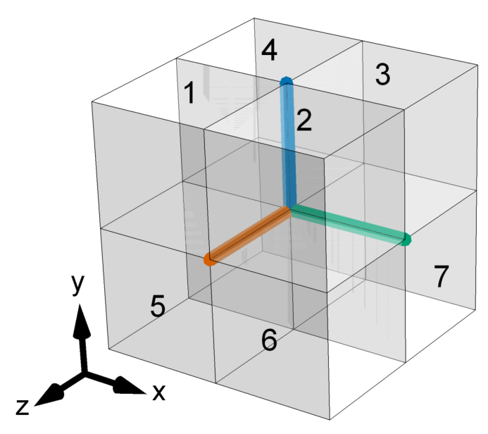
A 3+1D topological defect network is a particular instance of a defect TQFT that lives on a “stratified” 3-manifold $\mathcal{M}$ . A stratification consists of collections $S_{j}$ ( $j\in[0,3]$ ) of $j$ -dimensional submanifolds that decompose the manifold, as in Fig. 1. Elements of $S_{j}$ are referred to as $j$ -strata. We assign a 3+1D TQFT to each 3-strata and associate a topological defect with each $j$ -stratum (for $j<3$ ), thereby coupling together the ambient TQFTs. This coupling, mediated by the defect network, underpins the flexibility of topological defect networks as it directly imposes the mobility constraints characteristic of fracton models. In particular, this coupling dictates the set of topological excitations that condense on a given $j$ -strata and hence, along with the braiding data already encoded in the 3+1D TQFT, determines the set of excitations which cannot pass through that strata—any excitations which braid non-trivially with any of the condensed excitations on a defect are prohibited from passing through it.

The Hamiltonian for a topological defect network can be written schematically as

H=\sum_{j=0}^{3}H_{j}\,,

(1)

where $H_{j}$ is associated with terms in the Hamiltonian acting on degrees of freedom localized near a $j$ -strata. Although we restrict our attention to cubic lattices in this work, topological defect networks are defined for arbitrary stratifications of manifolds; likewise, while we only consider translation invariant models here, we see no obstruction to defining topological defect networks even outside this context.

While in principle subsumed under defect TQFTs, topological defect networks nevertheless provide a novel framework as they are comprised of an extensive network of topological defects enmeshed in a TQFT, and, as we show in this paper, are capable of describing gapped fracton phases. We remark also that our construction differs from earlier layered constructions of fracton models Ma et al. 2017; Vijay 2017; Vijay and Fu 2017; Prem et al. 2019; Slagle and Kim 2017a, where layers of coupled 2+1D topological orders were driven into a fracton phase through a condensation transition and the effective Hamiltonian was determined perturbatively. In the defect network picture, no such transition is required since the fracton phase is entirely determined by the choice of 3+1D TQFT and the network of defects it is immersed in. Thus, a significant virtue of this framework is that it allows one to write down exact commuting projector Hamiltonians (assuming the strata are non-chiral), thereby providing a constructive approach to discovering new fracton models.

Figure 2: A 2-stratum defect layer (black line) in the string-membrane-net model, which is embedded in a 3+1D toric code. The 3d toric code has charge (labeled

e

) and flux string (red lines in figure) excitations. The defect layer also supports 2d toric code charge (labeled

e^{\prime}

) and point-like flux (labeled

m^{\prime}

) excitations. The following excitations can be created near a defect layer using local operators: (a) a 2d toric code charge

e^{\prime}

and a 3d toric code charge on each side of the defect layer; (b) a pair of 2d toric code fluxes

m^{\prime}

at the endpoints of a 3d toric code flux string; and (c) a closed 3d toric code flux string.

The key concepts underlying topological defect networks are captured by a simple example that realizes a phase equivalent to that of the X-Cube model. Consider three stacks (along the $xy$ -, $yz$ -, and $xz$ -planes) of 2-strata layers embedded into a 3+1D toric code. Each 2-strata defect consists of a 2+1D toric code, coupled strongly to the 3+1D toric code living on the 3-strata. The coupling between the 3– and 2-strata can be characterized in terms of the topological excitations which can locally be created in the vicinity of the 2-strata defects; these excitations are summarized in Fig, 2. The mobility constraints imposed by this choice of 2-strata defects are described in Fig. 3. In fact, the string-membrane-net model Slagle et al. 2019b turns out to be secretly describing precisely this topological defect network, as the field theory discussed in that context can be suitably modified to fit the defect picture (see Appendix A). More generally, as we show in this paper, ground state wavefunctions of topological defect networks are fluctuating string-membrane-net configurations.

Figure 3: Stacks of 2-strata defect layers (defined in Fig. 2) result in the fracton and lineon mobility constraints of the X-Cube model. (a) The defect layers cause the 3d toric code charge (labeled

e

) to obtain fracton-like mobility. To see this, consider (i) trying to move a 3d charge

e

to move through a bunch of layers. (ii) This can only be done by creating the triplets of charges in Fig. 2(a) on the defect layers. (iii) Pairs of 3d charges

e

can annihilate, but a string of 2d charges

e^{\prime}

are left behind. This string of excitations linearly confines the 3d charge

e

to its initial location, just like an X-Cube fracton. (b) A lineon results from a pair of 2d toric code fluxes

m^{\prime}

(which are bound to the endpoints of a 3d toric code flux) on two intersecting defect layers.

Main Results

In this work, we argue that all types of gapped fracton models can be realized by topological defect networks, thereby demonstrating that these models can, in fact, be described in the language of defect TQFT. We proceed mostly by example and construct concrete examples of topological defect networks for well-known gapped fracton models, including the X-Cube and Haah’s B code, as well as a fractal type-I model. Besides these, we also present a new non-Abelian fracton model based on 3+1D $D_{4}$ gauge theory, which hosts fully immobile non-Abelian excitations.

Although we do not rigorously prove that all gapped fracton phases can be constructed from a topological defect network, we strongly expect this to be true, especially given the plethora of models that fit within this framework. Furthermore, it has previously been shown that networks of invertible defects can be used to construct crystalline SPT (cSPT) orders Else and Thorngren 2019; Song et al. 2017; Huang et al. 2017, which are SPT orders that are protected by spatial symmetries. This suggests that defect networks should also be capable of describing symmetry enriched topological and fracton orders. Of course, defect networks can trivially realize any TQFT by simply not embedding any defects within the TQFT.

Since the aforementioned phases appear to exhaust all known zero-temperature gapped phases of matter, we are motivated to make the following conjecture:

Conjecture.

Topological defect networks realize all zero-temperature gapped phases of matter.

That is, for every zero-temperature gapped phase of matter, we conjecture that there exists a topological defect network with a Hamiltonian whose ground state is within that phase. However, we add the caveat that the correct notion of “phase of matter” is still somewhat controversial for fracton phases. Nevertheless, we expect the conjecture to hold for any reasonable definition of a phase, such as phases up to adiabatic deformation or up to local unitary equivalence Chen et al. 2010. Assuming this conjecture, we further argue that there are no stable translation invariant gapped type-II fracton phases of matter in 2+1D.

This paper is organised as follows: In Sec. II, we build a topological defect network description of the X-Cube model and show that this naturally leads to a membrane-net description of its ground state wavefunction. In Sec. III, we construct Haah’s B code, a type II fracton model with no mobile excitations, within the defect picture. In Sec. IV, we build on these ideas to construct a new fracton model based on a network of defects embedded in a $D_{4}$ lattice gauge theory, and we show that the mobility constraints imposed by this network imply the presence of fully immobile non-Abelian fractons. So as to keep our discussion accessible to non-experts, various technical details regarding these three models have been relegated to Appendices D, E, and F respectively. In Sec. V, we present an argument that 2+1D topological defect networks cannot produce stable type-II fracton phases, and conclude with a discussion of open questions and future directions in Sec. VI. In Appendix A we outline a field theory description of the defect networks for string-membrane-net models; in Appendix B we describe a topological defect network construction of a fractal lineon model Yoshida 2013; Castelnovo and Chamon 2012; and in Appendix C we describe a topological defect network construction of a $\mathbb{Z}_{3}$ type-I model from trivial 3-strata.

II X-Cube from Topological Defects in 3+1D Toric Code

In this section we use the conceptual picture outlined in the introduction to realize the X-Cube model. This example is similar to the string-membrane-net example discussed in the introduction (and Fig. 2 and 3), except now we will not have $e^{\prime}$ or $m^{\prime}$ excitations on the boundary layer. This will result in simpler 2-strata defects, but more complicated 1-strata defects. The model is realized by three stacks of defect layers, which live in an ambient 3+1D toric code phase (see Fig. 1). In the following three subsections, we describe the construction in two complementary ways. The first approach defines the construction in terms of the excitations which are condensed on the defects, and makes the mobility constraints of the fracton and lineon excitations most explicit. The second defines the ground state wavefunction as a superposition of allowed membrane-net configurations. In App. D, we provide a concrete lattice Hamiltonian that explicitly realizes this defect network.

II.1 3+1D toric code preliminaries

The 3d toric code plays an essential role in the topological defect network construction of the X-Cube model. In this subsection, we briefly review the 3d toric code on the cubic lattice.

We will take the degrees of freedom to live on the plaquettes, such that the total Hilbert space is a tensor product of one spin-1/2 per plaquette. The Hamiltonian is a sum of two terms Castelnovo and Chamon 2008:

\displaystyle H=-J_{e}\sum_{e}A_{e}-J_{c}\sum_{c}B_{c}.

(2)

Where $\sum_{e}$ runs over all edges and $\sum_{c}$ runs over all cubes of the cubic lattice. The first term is given by

\displaystyle A_{e}=\prod_{p\in e}Z_{p},

(3)

where $p\in e$ denotes all plaquettes $p$ with a common edge $e$ . The second term is given by

\displaystyle B_{c}=\sum_{p\in\partial c}X_{p},

(4)

where $p\in\partial c$ denotes all plaquettes on the boundary of a cube $c$ . All terms in the Hamiltonian (2) commute, and so the model is exactly solvable. The ground space is given by any state satisfying $A_{e}|\psi\rangle=B_{c}|\psi\rangle=|\psi\rangle$ for all edges $e$ and cubes $c$ .

The 3d toric code has particle excitations, denoted $e$ , which consist of a single cube where $B_{c}$ has eigenvalue $-1$ . A pair of particle excitations are created at the end points of a string operator which is given by $\prod_{p\in\ell}Z_{p}$ , where $\ell$ is a path on the dual lattice, and $p\in\ell$ are all plaquettes which intersect that path. The 3d toric code also has flux loop excitations, denoted $m$ , consisting of a loop of edges where $A_{e}$ has eigenvalue $-1$ . A flux loop is created at the boundary of a membrane operator given by $\prod_{p\in S}X_{p}$ , where $S$ is a surface, and $p\in S$ are all plaquettes contained in that surface.

For later use, we now describe the 3+1D toric code with a boundary. There are two natural boundary conditions; the ‘‘rough” boundary which condenses flux loops, and the ‘‘smooth” boundary which condenses the particle excitations.⁶⁶ 6 In fact, any $\mathbb{Z}_{2}$ graded fusion category provides a natural boundary condition for the 3+1D toric code. In the following, we focus on the flux condensing boundary, typically referred to as the rough boundary since it consists of dangling plaquettes. That is, we terminate the cubic lattice on a surface (for example, a plane) and remove all plaquettes which reside in that plane. In the bulk, the Hamiltonian remains un-modified taking the form of (2). The sums in (2) are now over all edges which are not in the surface, and all cubes which do not meet the surface. The boundary Hamiltonian is given by

\displaystyle H_{\text{boundary}}=-J_{c}^{\prime}\sum_{c\in\text{boundary}}B_{c}^{\prime}

(5)

where

\displaystyle B_{c}^{\prime}=\prod_{p\in c}X_{p},

(6)

and ‘ $c\in\text{boundary}$ ’ denotes all cubes which share one (or more) plaquettes with the boundary. The boundary is said to condense flux loops, since a membrane operator which terminates on the boundary does not violate any terms in the Hamiltonian. Electric excitations remain as excitations when brought to the boundary.

The ground state wavefunction can be viewed as a condensate of membranes. To do so, one associates $Z_{p}=-1$ with a membrane present on plaquette $p$ . The condition $A_{e}=+1$ enforces that the membranes are closed, and $B_{c}=+1$ forces all possible closed membrane configurations to appear in the wavefunction with equal amplitude. On a flux condensing boundary, we relax the first of these conditions and allow membranes to terminate on the boundary. The term $B_{c}^{\prime}$ then forces the ground state to be an equal weight super position of all such allowed membrane configurations.

In the following section we will use a mild generalization of these gapped boundaries to construct the X-Cube model out of a lattice of 3+1D toric codes coupled together by defects.

II.2 Condensation on defects

We now describe the topological defects used to construct the X-Cube model by the excitations that condense on them. For simplicity we write the Hamiltonian on the 3-torus. We choose a stratification of the 3-torus to be a cubic lattice, where the cubes are the 3-strata, the plaquettes are the 2-strata, the edges are the 1-strata, and the vertices are the 0-strata (see Fig. 1). When constructing a lattice model, we use a cell decomposition of the stratified 3-torus given by a smaller lattice, as also shown in Fig. 1. The topological defects are used to couple the 3+1D toric codes on the 3-strata in such a way that the resulting theory is equivalent to the X-Cube model. In the following we describe the defects assigned to the 2- and 1-strata by the particles which condense on them.

We first look at the 2-strata defects. Each 2-stratum is neighbored by a pair of 3-strata, and the 2-stratum defect is characterized by the excitations that condense on it. With the benefit of hindsight, the excitations which condense on each 2-stratum are generated by the flux loops from the neighboring 3-strata

\displaystyle\{m_{+},m_{-}\},

(7)

where $m_{+}$ is from one toric code and $m_{-}$ is from the other. That is, the defect independently condenses the flux loop excitations from both neighboring 3-strata. This boundary condition forbids the $e$ particles from passing through the 2-strata, thus imposing mobility restrictions necessary for a fracton phase.

Next we zoom in on the 1-strata. These live at the junction of four 2- and 3-strata. Consequently, we need to specify which 3-strata and 2-strata excitations condense on the 1-strata. In this example, the 2-strata excitations are simply $e$ particles brought from the bulk to the boundary. Thus we only need to specify how the 3-strata excitations condense on the 1-strata, since this determines how the 2-strata excitations condense on the 1-strata.

The 2-strata defects we have chosen are very special and readily allow us to apply a dimensional reduction trick to understand the 1-strata defects. Near a 1-stratum, each 3-stratum toric code gets pinched into a very thin slab. In the thin slab, the low energy excitations are given by $e$ particles as before, and short $m$ -strings connecting both sides of the slab, effectively realizing a 2+1D toric code, as illustrated in Fig. 4.

Figure 4: When the 2-stratum condense all fluxes, the 1-strata boundary conditions can be understood using a dimensional reduction trick. In (a) we depict how membranes near a 1-strata effectively behave as strings in a dimensionally reduced 2+1D toric code. In (b) we show how the 3-strata excitations map onto the dimensionally reduced toric code excitations.

Hence, we can understand the 1-strata defects from condensation processes of the dimensionally reduced 3d toric codes. At the 1-stratum defect, we condense quadruples of $e$ particles and all pairs of fluxes coming from the neighboring 3d toric codes. These are generated by

\displaystyle\{m_{1}m_{2},m_{2}m_{3},m_{3}m_{4},e_{1}e_{2}e_{3}e_{4}\}\,,

(8)

where 1, 2, 3, and 4 denote the four neighboring 3-strata. (The ordering does not matter.) One can check that the algebra object generated by the above particles is a Lagrangian algebra object for the boundary of the four (effectively) 2d toric codes meeting at the 1-stratum, and therefore no further particles need to be condensed in order to have a gapped 1-stratum.⁷⁷ 7 If $A$ is the algebra object being condensed, then it is Lagrangian if $(\text{dim}\;A)^{2}=\text{dim}\;\mathcal{D}(\mathbb{Z}_{2}^{4})$ . There are $2^{4}=16=\text{dim}\;A$ particles generated by (8). We also have $\text{dim}\;\mathcal{D}(\mathbb{Z}_{2})=4$ , and so $\text{dim}\;\mathcal{D}(\mathbb{Z}_{2}^{4})=4^{4}=(\text{dim}\;A)^{2}$ .

The data on higher strata do not uniquely determine a defect on the 0-strata. For example, the 0-strata could pin topological excitations from the various $3-$ , $2-$ and $1-$ strata which meet at the 0-strata. To obtain the X-Cube model, we choose the 0-strata defects to not pin any topological charges from the neighboring 3-, 2- and 1-strata.

We have now finished describing all data needed to specify the defects. In the following section, we analyze the character of the topological excitations, and in the subsequent section, we write down an explicit membrane-net condensate.

II.3 Mobility Constraints

We now analyze the excitations present in this defect construction and verify that they enjoy mobility constraints typical of fracton phases. In particular, we show that their mobility constraints are consistent with those of topological excitations in the X-Cube model.

The charge excitations $e$ cannot move through the 2-strata since the flux excitations are condensed there. However, due to the 1-stratum condensation [Eq. (8)], four charges can be created on four neighboring 3-strata [Fig. 5(a)]. As a result, the charge excitations $e$ have exactly the same mobility constraints as the fractons in the X-Cube model. Furthermore, if two $e$ are in the same $3$ -stratum, they can be fused to the identity, in the same way that two fractons on the same cube in the X-Cube model fuse to the identity.

A lineon excitation results from a flux string that ends on two neighboring 2-strata; see Fig. 5(b). This excitation cannot be annihilated by simply shrinking the string since single flux excitations are not condensed on the 1-strata; only pairs of flux strings on neighboring 3-strata are condensed [Eq. (8)]. Similar to X-Cube lineons, three lineons can be locally created from the vacuum, as shown in Fig. 5(c). In Fig. 5(d-f), we show more explicitly how the condensations on the $1$ -strata allow this excitation to move like an X-Cube lineon.

Also as in the X-Cube model, planons result from pairs of fractons (charges $e$ in this model) or lineons. The lineon pair is equivalent to an m-string which is orthogonal to the mobility plane.

II.4 Nets and Relations

In this subsection, we present the X-Cube model as a network of defects in the membrane-net condensate picture of the 3+1D toric code. In this picture, we present “allowed” membrane configurations and linear relations amongst those membranes. The ground state wavefunction is a weighted superposition of all allowed membrane configurations:

\displaystyle|{\Psi}\rangle=\sum_{\text{M}}\phi(\text{M})|\text{M}\rangle.

(9)

In the above, “M” denotes an allowed membrane configuration, and $\phi(\text{M})$ is the weighting which is determined by the linear relations on the membranes. In the following, $\phi(\text{M})=+1$ for all allowed diagrams.

We specify whether a net diagram is “allowed” by checking whether it locally satisfies some admissibility constraints. We begin by describing the admissible membranes on the interior of a 3-strata, followed by the allowed membranes near the 2-, 1-, and 0-strata. Excitations correspond to violations of the “allowed” membrane configurations or changes to the phases $\phi(\text{M})$ in (9).

3-strata

We first specify the allowed membranes which reside on the interior of a 3-stratum. These are given by surfaces which are locally closed. That is, if we choose a closed path in the interior of a 3-stratum, the path must intersect an even number of surfaces. For example,

\displaystyle\mathord{\vbox{\hbox{\includegraphics[scale]{cupcapprime.pdf}}}}\;=\;\;\mathord{\vbox{\hbox{\includegraphics[scale]{cylinderprime.pdf}}}}\,,

(10)

and so the two configurations appear with equal amplitude in the wavefunction.

2-strata

The 2-strata defects are given by rough boundary conditions for the the two adjacent 3-strata toric codes. That is, we allow membranes from the neighboring 3-strata toric codes to freely terminate on the 2-strata. Hence, near a 2-stratum, a generic membrane configuration and linear relation looks like:

\displaystyle\mathord{\vbox{\hbox{\includegraphics[scale]{twocellnetaprime.pdf}}}}=\mathord{\vbox{\hbox{\includegraphics[scale]{twocellnetbprime.pdf}}}}

(11)

1-strata

The 1-strata defects can be inferred from the dimensional reduction picture described in Sec. II.2. The fact that pairs of any two fluxes can condense on the 1-strata tells us that we must have an even number of membranes terminating on each 1-stratum. A top view of the allowed membrane configurations is shown in Fig. 6.

Figure 6: A representative set of allowed membrane configurations near a 1-cell as viewed from above (i.e., down a 1-cell). The remaining allowed configurations come from rotating the two diagrams on the right.

0-strata

A membrane configuration near a 0-stratum is “allowed” if it satisfies the constraints imposed by the 1- and 2-strata defects when pulled away from the 0-stratum. That is, membranes near the 0-strata do not pick up any additional constraints not already imposed by the 1- and 2-strata defects.

In App. D, we explicitly write out a Hamiltonian whose ground state can be viewed as an equal weight superposition of the allowed membrane configurations described in this section.

III Haah’s B Code from Topological Defects

In this section, we show that Haah’s B code Haah 2014, which is a so-called “type-II” fracton model in which all topologically non-trivial excitations are immobile and created by operators with fractal support, can also be realized using a defect network in an ambient 3+1D $\mathbb{Z}_{2}\times\mathbb{Z}_{2}$ toric code. We first briefly review the B code before describing the defect network.

III.1 Review of Haah’s B code

The Hilbert space of Haah’s B code consists of four qubits per site of a cubic lattice. We use a shorthand where, for example, $XZXZ$ means applying a Pauli $X$ operator to the first and third qubit on a given site and a Pauli $Z$ operator to the second and fourth qubits on that site. The Hamiltonian is

H=-\sum_{c}\left(A_{c}+B_{c}+C_{c}+D_{c}\right)

(12)

where $c$ is an elementary cube in the lattice and $A_{c}$ , $B_{c}$ , $C_{c}$ , and $D_{c}$ are products of Pauli operators shown in Fig. 7.

$A_{c}$

$B_{c}$

$C_{c}$

$D_{c}$

Figure 7: Terms in the Hamiltonian for Haah’s B code, which has four qubits per site of the cubic lattice.

X

and

Z

are Pauli operators,

I

is the identity, and the shorthand

XXXX

(for example) means a product of Pauli X operators on all four qubits on the site in question.

It is straightforward to check that all terms in the Hamiltonian mutually commute. Hence, in the ground state(s), every term has eigenvalue $+1$ . Elementary excitations consist of cubes on which one or more of these four terms have eigenvalue $-1$ .

Local operators acting on ground states can easily be checked to create excitation configurations such as those in Fig. 8a. These patterns are such that certain operators with fractal-like support, such as the one in Fig. 8b, can create isolated excitations at their corners. We will show in the next subsection that a defect construction can admit local operators which create excitations in the same patterns as the ones shown here.

III.2 Condensation on defects

The defect construction uses the same stratification of space shown in Fig. 1, that is, a cubic lattice of 3-strata. Each 3-stratum contains a $\mathbb{Z}_{2}\times\mathbb{Z}_{2}$ gauge theory, that is, two copies of the 3+1D toric code. Each 3-stratum therefore contains two types of electric charges, which we label $e^{A}$ and $e^{B}$ ; two types of magnetic string excitations $m^{A}$ and $m^{B}$ ; and the bound states of these objects. Intuitively, a 3-stratum in the defect picture containing an odd number of $e^{A}$ (resp. $e^{B}$ ) will correspond to a unit cube with $A_{c}=-1$ (resp. $B_{c}=-1$ ) in Haah’s B code, while the $m^{A}$ (resp. $m^{B}$ ) excitations will, in a more subtle way, correspond to unit cubes with $C_{c}=-1$ (resp. $D_{c}=-1$ ). This is why we choose to start from two copies of the 3+1D toric code in each unit cell instead of one.

Each 2-stratum borders two 3-strata containing a $\mathbb{Z}_{2}\times\mathbb{Z}_{2}$ 3d toric code. We declare that all $m$ excitations in either 3-stratum can condense on the 2-strata, i.e., a generating set of local excitations on the defects is

\{m^{A}_{+},m^{A}_{-},m^{B}_{+},m^{B}_{-}\}

(13)

where the $+$ excitations are from one $\mathbb{Z}_{2}\times\mathbb{Z}_{2}$ toric code and $-$ is from the other. This ensures that no point-like objects can pass freely through the 2-strata.

On the 1-strata, we allow some bulk excitations to condense. Generating sets of the condensed excitations consist of:

$\displaystyle\{e^{B}_{2}e^{A}_{3}$	$\displaystyle e^{B}_{3}e^{A}_{6},e^{A}_{2}e^{B}_{2}e^{A}_{3}e^{B}_{6},m^{A}_{2}m^{B}_{6},m^{B}_{2}m^{A}_{3},m^{B}_{3}m^{A}_{6},m^{B}_{2}m^{A}_{6}m^{B}_{6},m^{A}_{7},m^{B}_{7}\}\hskip 14.22636pt\text{ ($x$-oriented 1-stratum)}$	(14)
$\displaystyle\{e^{A}_{1}e^{B}_{1}$	$\displaystyle e^{B}_{2}e^{A}_{3},e^{A}_{1}e^{A}_{2}e^{B}_{2}e^{B}_{3},m^{A}_{1}m^{B}_{2},m^{B}_{1}m^{A}_{3},m^{A}_{2}m^{B}_{3},m_{1}^{A}m_{1}^{B}m_{3}^{B},m^{A}_{4},m^{B}_{4}\}\hskip 14.22636pt\text{ ($y$-oriented 1-stratum)}$	(15)
$\displaystyle\{e^{A}_{1}e^{B}_{1}$	$\displaystyle e^{A}_{2}e^{B}_{6},e^{A}_{1}e^{B}_{2}e^{A}_{6}e^{B}_{6},m^{A}_{1}m^{B}_{6},m^{B}_{1}m^{A}_{2},m^{B}_{2}m^{A}_{6},m^{A}_{1}m^{B}_{1}m^{A}_{6},m^{A}_{5},m^{B}_{5}\}\hskip 14.22636pt\text{ ($z$-oriented 1-stratum)}$	(16)

The subscripts label 3-strata according to Fig. 9, in which the links on which we are specifying condensations are colored green, blue, and orange, respectively. Using the dimensional reduction trick (see Fig. 4), it is easy to check that these condensations yield a gapped boundary. Alternatively, this will be clear when discussing the nets and relations picture of the B code defect construction.

Finally, the 0-strata defects are chosen to not pin any topological charges from the neighboring higher strata.

The data on the 1-strata is fairly complicated, so we presently explain it by examining the excitations in this model. We have chosen the condensed electric charges to match the action of local operators in Haah’s B code in the following sense. Under the aforementioned correspondence where a 3-stratum containing an odd number of $e^{A}$ (resp. $e^{B}$ ) is to be thought of as a cube in the B code with $A_{c}=-1$ (resp. $B_{c}=-1$ ), the statement that $e^{B}_{2}e^{A}_{3}e^{B}_{3}e^{A}_{6}$ is condensed (i.e. can be created locally) at an $x$ -oriented 1-stratum corresponds to the fact that, in Haah’s B code, the operator $ZIII$ creates the pattern of excitations in Fig. 8a. This correspondence is shown pictorially in Fig. 10a. Likewise, the condensation of $e^{A}_{2}e^{B}_{2}e^{A}_{3}e^{B}_{6}$ and $e^{A}_{2}e^{B}_{3}e^{A}_{6}e^{B}_{6}$ , respectively, correspond to the actions of $IZII$ and $ZZII$ in Haah’s B code. It is straightforward to check that every condensed electric charge in the defect construction corresponds to a local product of Pauli $Z$ operators in Haah’s B code. These condensations also permit the creation of widely separated excitations using networks of string operators whose support is fractal-like. An example which corresponds to the B code excitation pattern created in Fig. 8b is shown in Fig. 10b.

The magnetic excitations are created by applying open membrane operators whose boundaries lie entirely on the boundaries of 3-strata. Since $m$ excitations are condensed on the 2-strata, excitations only occur when the membrane operators intersect 1-strata in certain patterns. The most convenient membrane operators to investigate are those which lie parallel to a 2-stratum, an example of which is shown in Fig. 11a. Due to the condensation of $m^{A}_{4}$ and $m^{B}_{4}$ in Eq. (15) (see Fig. 9 for labeling), the front-most $y-$ oriented link in Fig. 11a does not have an excitation on it, while the other three $y$ -oriented links do because single $m$ excitations in this 3-stratum are not condensed on those links. (We will shortly explain why we have labeled the excitations with B code labels $C$ and $D$ .) However, since some $m$ bound states are condensed on the 1-strata, applying several such membrane operators on neighboring 3-strata can remove these excitations provided the layers of the membrane operators are chosen carefully. For example, the fractal-like membrane operator in Fig. 11b creates three widely separated excitations with nothing in between. These patterns of excitations are exactly the ones which can be created in the B code using patterns of Pauli $X$ operators analogous to those shown for Pauli $Z$ operators in Fig. 8b.

We now explain how we identify the excitations created by magnetic membranes on the 1-strata. Using the correspondence between local Pauli $Z$ operators and the creation of condensed electric particles on the 1-strata, illustrated for example in Fig. 10a, we can represent the action of $C_{c}$ and $D_{c}$ as creating certain condensed sets of electric particles at the 1-strata and annihilating pairs inside the 3-strata, that is, as a complicated set of closed toric code electric string operators.

These string operators are shown in Fig. 11c. These string operators anticommute with some of the membrane operators in question. For example, if the B-layer membrane operator in Fig. 11a lives in cube 5 (using the same labeling as Fig. 9) in Fig. 11c, it will anticommute with the $D_{c}$ operator on the highlighted cube (cube 8) but will commute with the $C_{c}$ operator on that cube. Hence the $m^{B}$ operator in question creates a $D_{c}$ excitation on cube 8. To obtain the labeling in Fig. 11a, we must associate this B code excitation in a 3-stratum to a 1-stratum. Such a correspondence arises from the fact that in Fig. 11c, string operators only act on three of the twelve 1-strata that border the highlighted 3-stratum, one of each orientation. It is easy to check that each 1-stratum is involved only in a single $C_{c}$ operator and a single $D_{c}$ operator. In this sense, magnetic excitations on a 1-stratum can be uniquely assigned to a 3-stratum. In this way, the excitation labeled $D$ in Fig. 11a in the defect construction language can be associated to a $D_{c}$ excitation on cube 8 in the B code language. One can further check that there exist membrane operators which move magnetic excitations between the three 1-strata associated to the same cube (but not to any other 1-strata) without creating additional excitations, which is why the correspondence between 3-strata and 1-strata is not one-to-one.

III.3 Nets and relations

In this subsection, we explain the condensation picture of the previous subsection in terms of membrane-net diagrams and relations on them.

The ground state wavefunction in our construction can be written as a superposition

|{\Psi}\rangle=\sum_{\text{M}}\phi(\text{M})|\text{M}\rangle.

(17)

where $M$ is a membrane configuration and $\phi(M)$ is the weighting determined by linear relations on the membranes. For our case, $\phi(M)=+1$ for allowed net-diagrams and $\phi(M)=0$ otherwise. Since the ambient topological order is the bilayer 3+1D toric code, there are two membrane colors, which we refer to as orange and blue. As before, “allowed” net-diagrams are those which satisfy constraints which we specify presently.

The 3-stratum constraint is that each color of membrane is locally closed independently, that is, closed paths on the interior of a 3-stratum must intersect an even number of surfaces of each color. In the presence of a 2-stratum defect, membranes of either color may end freely on the 2-stratum without constraint. That is, we independently impose the same 3- and 2-stratum constraints used in the X-Cube construction on each color of 3d toric code.

The 1-strata have constraints which couple the two membrane colors. Each 1-stratum interfaces with four 3-stratum bilayer toric codes. The set of membranes which may freely terminate on a 1-stratum is given by the set of $m$ particles which are condensed in Eqs. (14)-(16), where $m^{A}$ (resp. $m^{B}$ ) corresponds to an orange (resp. blue) net. A generating set of allowed configurations for the $x$ -oriented 1-strata are shown in Fig. 12; the allowed configurations on the other 1-strata are obtained analogously.

Any membrane configuration surrounding a 0-stratum which satisfies the 1-, 2-, and 3-stratum constraints is admissible.

In Appendix E, we construct an exactly solvable Hamiltonian for our defect network construction of Haah’s B code. Our arguments from this section, along with the exactly solvable model, demonstrate the fact that our construction can indeed realize type-II fracton models; we will demonstrate in the next section that we can also realize models with non-Abelian fractons.

IV Non-Abelian fracton model from topological defects in 3+1D $D_{4}$ gauge theory

The defect picture developed for the X-Cube model in Section II provides a roadmap for building new fracton models, including those hosting non-Abelian excitations with restricted mobility. In this section, we discuss a defect network construction for a non-Abelian fracton model based on $D_{4}$ gauge theory, distinct from non-Abelian fracton models that have previously appeared in the literature. Similar to the X-Cube defect network, the model is constructed from three stacks of coupled defect layers within an ambient 3+1D $D_{4}$ gauge theory bulk. The defect layers serve to restrict the mobility of the non-Abelian bulk particle, thereby promoting it to a fracton. We follow the previous sections by first describing the construction in terms of excitations condensing on defects, and secondly in terms of superpositions of allowed configurations appearing in the ground state wavefunction. In App. F we describe a local lattice Hamiltonian that realizes the non-Abelian topological defect network construction of this section.

IV.1 Review of $D_{4}$ gauge theory

The group $D_{4}$ corresponds to the symmetries of a square and is specified by

\displaystyle D_{4}=\left\langle r,s\,\large|\,r^{2}=s^{4}=rsrs=1\right\rangle\,,

(18)

with center given by $\langle s^{2}\rangle$ . There are five conjugacy classes $\{1\}$ , $\{s^{2}\}$ , $\{s,s^{3}\}$ , $\{r,rs^{2}\}$ , $\{rs,rs^{3}\}$ , and hence five irreducible representations (irreps): four of dimension one and one of dimension two. The character table is given by

	$1$	$s^{2}$	$s$	$r$	$rs$
$\chi_{00}$	1	1	1	1	1
$\chi_{01}$	1	1	$-1$	1	$-1$
$\chi_{10}$	1	1	1	$-1$	$-1$
$\chi_{11}$	1	1	$-1$	$-1$	1
$\chi_{\sigma}$	2	$-2$	0	0	0

Notice that the first four irreps obey the obvious $\mathbb{Z}_{2}\times\mathbb{Z}_{2}$ fusion rules, while

\displaystyle{ij}\otimes\sigma=\sigma\,,

\displaystyle\sigma\otimes\sigma=\sum_{i,j}ij\,,

(25)

obey a $\mathbb{Z}_{2}$ grading, where $i,j\in\mathbb{Z}_{2}$ . Physically, the $\mathbb{Z}_{2}$ grading on the particles is induced by their braiding with the Abelian $s^{2}$ loop excitation. The non-trivial $F$ -symbols of the fusion category Rep $(D_{4})$ are given by

\displaystyle[F_{k\ell}^{\sigma\,ij\,\sigma}]^{\sigma}_{\sigma}=[F_{\sigma}^{ij\,\sigma\,k\ell}]^{\sigma}_{\sigma}=2\,[F_{\sigma}^{\sigma\sigma\sigma}]^{ij}_{k\ell}=(-1)^{ik+j\ell}\,.

(26)

Rep $(D_{4})$ furthermore admits a trivial braiding.

In three spatial dimensions, the pointlike gauge charges of $D_{4}$ gauge theory are described by Rep $(D_{4})$ and the looplike flux excitations are locally labelled by the conjugacy classes of $D_{4}$ Dijkgraaf and Witten 1990. The pointlike charges can be measured by braiding flux loops around a charge, while the looplike fluxes can be measured by braiding charges around a loop. The braiding phase between an irrep labelled charge and a conjugacy class labelled flux is given by the phase of the corresponding entry in the the character table above.⁸⁸ 8 For example, the wave function picks up a minus sign if the $11$ charge is braided with the $\{s,s^{3}\}$ flux, or if the $\sigma$ charge is braided with the $s^{2}$ flux.

IV.2 Condensation on defects

In this section, we specify the defects used to construct our non-Abelian fracton model in terms of the excitations that condense on them. We again consider a cubic lattice stratification of the 3-torus with degrees of freedom living on a much finer grained cubic lattice. Cubes of $D_{4}$ gauge theory on the 3-strata with gapped boundaries are coupled together in a similar way to the X-Cube defect TQFT to achieve a model where the non-Abelian $D_{4}$ gauge charge is promoted to a fracton.

On the 2-strata, we introduce a topological defect on which the flux loop excitations labelled by $s^{2}$ condense, but no other topological excitations from single 3-strata condense. This has the effect of restricting the non-Abelian $\sigma$ particle from moving across the 2-strata (since $\sigma$ braids non-trivially with $s^{2}$ flux loops), while other uncondensed topological excitations are free to pass through. The full set of excitations condensing on the 2-strata are labelled

\displaystyle\{s^{2}_{+},\;s^{2}_{-},\;c_{+}c_{-},\;ij_{+}ij_{-}\}\,,

(27)

where $c_{\pm}$ runs over all conjugacy classes, $ij_{\pm}$ runs over the Abelian charges, and $\pm$ indicates which adjacent cube the topological excitations originate from, see Fig. 13.

Figure 13: A 2-stratum defect layer (black line) in the non-Abelian

D_{4}

model described in the main text. The defect allows

s^{2}

membranes to terminate on the 2-strata. The following excitations can be created near a defect layer using local operators: (a) pairs of Abelian charges labeled

ij

on opposite sides of the defect; (b) a flux arc labeled by the conjugacy class

s^{2}

, and (c) a flux loop on opposing sides of the defect labeled by the same conjugacy class

c

On the 1-strata, we pick a topological defect where the following excitations condense

\displaystyle\{s^{2}_{\alpha}s^{2}_{\beta},\;c_{1}c_{2}c_{3}c_{4},\;{ij}_{\alpha}{ij}_{\beta},\;\sigma_{1}\sigma_{2}\sigma_{3}\sigma_{4}\}\,.

(28)

Here, $c$ runs over all conjugacy classes; $ij$ runs over the Abelian irreps; and $\alpha\neq\beta$ run over the quadrants 1,2,3,4, see Fig. 14. We remark that when the non-Abelian excitation $\sigma_{1}\sigma_{2}\sigma_{3}\sigma_{4}$ is brought onto the 1-stratum, it can fuse into any of the Abelian topological charges labeled by $ij$ . For $ij\neq 00$ , the leftover particle is a 1-stratum excitation (however we note that such excitations can be moved off the 1-stratum as the $ij$ particles do not have any mobility constraints). Thus, only the vacuum channel of $\sigma_{1}\sigma_{2}\sigma_{3}\sigma_{4}$ is condensed at the 1-stratum.

We remark that we are forced to include $c_{1}c_{2}c_{3}c_{4}$ and ${ij}_{\alpha}{ij}_{\beta}$ in the condensate for consistency with the adjacent 2-strata. While the above condensing particles may not fully specify the defect, they suffice to understand the properties of the fracton model thus constructed. We provide a full description of the defect in terms of nets and relations in Sec. IV.4, and an explicit lattice model in App. F.

(a)

(b)

(c)

(d)

Figure 14: A representative set of 1-stratum condensations described by Eq. (28). (a) Four non-Abelian

\sigma

charges can simultaneously condense to the vacuum on a 1-stratum. (b) The Abelian charges labeled

ij

are allowed to freely pass through the 2- and 1-strata. (c) Any pair of

s^{2}

flux strings can condense at the 1-strata. (d) Any quadruple of flux strings (labeled by a conjugacy class

c

) meeting at a 1-stratum can condense into vacuum.

The looplike excitations, $c$ , have a well-defined braiding with a 0-stratum that can detect the presence of a single (or an odd numbers of like) point charges there. Furthermore, there is a braiding process of an arclike $s^{2}$ excitation tracing out a hemisphere about the 0-stratum for each oriented axis $\pm\hat{x},\pm\hat{y},\pm\hat{z},$ that can detect an odd number of $\sigma$ charges above or below the ${yz},{xz},{xy}$ plane, respectively. Together, these braiding processes can detect $\sigma_{\alpha}\sigma_{\beta}$ pairs for $\alpha\neq\beta$ , but braid trivially with the $\sigma_{1}\sigma_{2}\sigma_{3}\sigma_{4}$ quadruples that condense on the 1-strata. On the 0-strata, we choose a topological defect that is trivial under the aformentioned braiding processes. This ensures that the defect does not induce any further condensation nor pin any pointlike topological excitations, including $\sigma_{\alpha}\sigma_{\beta}$ . This is easy to see for the Abelian particles, and for the non-Abelian particles utilizes the fact that a single $\sigma_{\alpha}$ particle picks up a sign under the $s^{2}$ braiding processes that pass through its octant.

IV.3 Mobility constraints

In this section, we analyze the mobility of the topological excitations in the $D_{4}$ defect network model. We demonstrate that the non-Abelian $\sigma$ particle, and arcs of the Abelian $s^{2}$ flux excitation obey similar constraints to the particle and flux excitations in the X-Cube defect network, respectively. On the other hand, the Abelian particles and non-Abelian flux loops remain fully mobile.

The non-Abelian $\sigma$ charge excitations cannot freely pass through the 2-strata since they braid non-trivially with the Abelian $s^{2}$ flux loops that condense there. Similar to the X-Cube defect network, they may be created in quadruples on the four 3-strata adjacent to a 1-strata, see Fig. 14(a). Furthermore, no additional mobility is endowed to the $\sigma$ particles by the defects on the 0-strata. Hence, the $\sigma$ excitations become non-Abelian fractons with analogous mobility to those in the X-Cube model.

An arc of Abelian $s^{2}$ flux between adjacent 2-strata can move along a line via the hopping process shown in Fig. 5(e-f). Shrinking any arc from a single quadrant onto the adjacent 1-strata leads to an equivalent excitation on the 1-strata. Three such excitations can be created in a 3-strata along the $\hat{x},\hat{y},$ and $\hat{z}$ axes, see Fig. 5(c). These properties lead to the same mobility as the X-Cube lineon excitations.

The Abelian $ij$ charges are fully mobile, as they can pass through the 2-strata due to the condensation of $ij_{+}ij_{-}$ there. Similarly, the non-Abelian $c$ flux loops excitations are fully mobile as they can pass through the 2-strata, due to the condensation of $c_{+}c_{-}$ there, and the 1-strata, due to the condensation of $c_{1}c_{2}c_{3}c_{4}$ there.

IV.4 Nets and relations

In this section we present a defect network construction of the non-Abelian $D_{4}$ fracton model, introduced in the previous subsections, in terms of a membrane-net condensate. Following Eq. (9) we describe allowed configurations of $D_{4}$ membranes on the various strata and the local relations between allowed configurations with the same coefficient in the wavefunction.

References

- Haah (2011) J. Haah, Phys. Rev. A 83, 042330 (2011).
- Chamon (2005) C. Chamon, Phys. Rev. Lett. 94, 040402 (2005).
- Castelnovo and Chamon (2012) C. Castelnovo and C. Chamon, Philosophical Magazine 92, 304 (2012), arXiv:1108.2051 .
- Kim (2012) I. H. Kim, (2012), arXiv:1202.0052 .
- Yoshida (2013) B. Yoshida, Phys. Rev. B 88, 125122 (2013).
- Haah (2014) J. Haah, Phys. Rev. B 89, 075119 (2014).
- Vijay et al. (2015) S. Vijay, J. Haah, and L. Fu, Phys. Rev. B 92, 235136 (2015).
- Vijay et al. (2016) S. Vijay, J. Haah, and L. Fu, Phys. Rev. B 94, 235157 (2016).
- Bravyi et al. (2011) S. Bravyi, B. Leemhuis, and B. M. Terhal, Annals of Physics 326, 839 (2011), arXiv:1006.4871 .
- Bravyi and Haah (2013) S. Bravyi and J. Haah, Phys. Rev. Lett. 111, 200501 (2013).
- Bravyi and Haah (2011) S. Bravyi and J. Haah, Phys. Rev. Lett. 107, 150504 (2011).
- Ma et al. (2017) H. Ma, E. Lake, X. Chen, and M. Hermele, Phys. Rev. B 95, 245126 (2017).
- Vijay (2017) S. Vijay, (2017), arXiv:1701.00762 .
- Vijay and Fu (2017) S. Vijay and L. Fu, (2017), arXiv:1706.07070 .
- Shirley et al. (2019a) W. Shirley, K. Slagle, and X. Chen, Annals of Physics 410, 167922 (2019a), arXiv:1806.08625 .
- Song et al. (2019) H. Song, A. Prem, S.-J. Huang, and M. A. Martin-Delgado, Phys. Rev. B 99, 155118 (2019).
- Bulmash and Iadecola (2019) D. Bulmash and T. Iadecola, Phys. Rev. B 99, 125132 (2019).
- Dua et al. (2019) A. Dua, D. J. Williamson, J. Haah, and M. Cheng, Phys. Rev. B 99, 245135 (2019).
- Kim and Haah (2016) I. H. Kim and J. Haah, Phys. Rev. Lett. 116, 027202 (2016).
- Prem et al. (2017) A. Prem, J. Haah, and R. Nandkishore, Phys. Rev. B 95, 155133 (2017).
- Williamson (2016) D. J. Williamson, Phys. Rev. B 94, 155128 (2016).
- You et al. (2018) Y. You, T. Devakul, F. J. Burnell, and S. L. Sondhi, Phys. Rev. B 98, 035112 (2018).
- Shirley et al. (2019b) W. Shirley, K. Slagle, and X. Chen, SciPost Physics 6, 041 (2019b).
- Schmitz (2019) A. T. Schmitz, Annals of Physics 410, 167927 (2019), arXiv:1809.10151 .
- Devakul et al. (2019) T. Devakul, W. Shirley, and J. Wang, (2019), arXiv:1910.01630 .
- Ibieta-Jimenez et al. (2019) J. P. Ibieta-Jimenez, L. N. Queiroz Xavier, M. Petrucci, and P. Teotonio-Sobrinho, (2019), arXiv:1908.07601 .
- Tantivasadakarn and Vijay (2019) N. Tantivasadakarn and S. Vijay, (2019), arXiv:1912.02826 .
- Brown and Williamson (2019) B. J. Brown and D. J. Williamson, (2019), arXiv:1901.08061 .
- Pretko (2017a) M. Pretko, Phys. Rev. B 95, 115139 (2017a).
- Pretko (2017b) M. Pretko, Phys. Rev. B 96, 035119 (2017b).
- Seiberg (2019) N. Seiberg, (2019), arXiv:1909.10544 .
- Pretko (2017c) M. Pretko, Phys. Rev. B 96, 125151 (2017c).
- Prem et al. (2018a) A. Prem, M. Pretko, and R. M. Nandkishore, Phys. Rev. B 97, 085116 (2018a).
- Ma et al. (2018a) H. Ma, M. Hermele, and X. Chen, Phys. Rev. B 98, 035111 (2018a).
- Bulmash and Barkeshli (2018) D. Bulmash and M. Barkeshli, Phys. Rev. B 97, 235112 (2018).
- Bulmash and Barkeshli (2018) D. Bulmash and M. Barkeshli, (2018), arXiv:1806.01855 .
- Williamson et al. (2019a) D. J. Williamson, Z. Bi, and M. Cheng, Phys. Rev. B 100, 125150 (2019a).
- Yan (2019) H. Yan, Phys. Rev. B 99, 155126 (2019).
- Wang and Xu (2019) J. Wang and K. Xu, (2019), arXiv:1909.13879 .
- Wang et al. (2019) J. Wang, K. Xu, and S.-T. Yau, (2019), arXiv:1911.01804 .
- Pretko and Radzihovsky (2018) M. Pretko and L. Radzihovsky, Phys. Rev. Lett. 120, 195301 (2018).
- Gromov (2019a) A. Gromov, Phys. Rev. Lett. 122, 076403 (2019a).
- Pai and Pretko (2018) S. Pai and M. Pretko, Phys. Rev. B 97, 235102 (2018).
- Kumar and Potter (2019) A. Kumar and A. C. Potter, Phys. Rev. B 100, 045119 (2019).
- Radzihovsky and Hermele (2020) L. Radzihovsky and M. Hermele, Phys. Rev. Lett. 124, 050402 (2020).
- Prem et al. (2018b) A. Prem, S. Vijay, Y.-Z. Chou, M. Pretko, and R. M. Nandkishore, Phys. Rev. B 98, 165140 (2018b).
- Yan et al. (2019) H. Yan, O. Benton, L. D. C. Jaubert, and N. Shannon, (2019), arXiv:1902.10934 .
- Sous and Pretko (2019) J. Sous and M. Pretko, (2019), arXiv:1904.08424 .
- Dubinkin et al. (2020) O. Dubinkin, J. May-Mann, and T. L. Hughes, (2020), arXiv:2001.04477 .
- He et al. (2019) H. He, Y. You, and A. Prem, (2019), arXiv:1912.10520 .
- Fuji (2019) Y. Fuji, Phys. Rev. B 100, 235115 (2019).
- Slagle and Kim (2017a) K. Slagle and Y. B. Kim, Phys. Rev. B 96, 165106 (2017a).
- Halász et al. (2017) G. B. Halász, T. H. Hsieh, and L. Balents, Phys. Rev. Lett. 119, 257202 (2017).
- Pai et al. (2019) S. Pai, M. Pretko, and R. M. Nandkishore, Phys. Rev. X 9, 021003 (2019).
- Sala et al. (2019) P. Sala, T. Rakovszky, R. Verresen, M. Knap, and F. Pollmann, (2019), arXiv:1904.04266 .
- Moudgalya et al. (2019) S. Moudgalya, A. Prem, R. Nandkishore, N. Regnault, and B. A. Bernevig, (2019), arXiv:1910.14048 .
- Nandkishore and Hermele (2019) R. M. Nandkishore and M. Hermele, Annual Review of Condensed Matter Physics 10, 295 (2019), arXiv:1803.11196 .
- Pretko et al. (2020) M. Pretko, X. Chen, and Y. You, (2020), arXiv:2001.01722 .
- Wen (2017) X.-G. Wen, Rev. Mod. Phys. 89, 041004 (2017).
- Moore and Seiberg (1989) G. Moore and N. Seiberg, Communications in Mathematical Physics 123, 177 (1989).
- Kitaev (2006) A. Kitaev, Annals of Physics 321, 2 (2006), arXiv:cond-mat/0506438 .
- Levin and Wen (2005) M. A. Levin and X.-G. Wen, Phys. Rev. B 71, 045110 (2005).
- Lan et al. (2018) T. Lan, L. Kong, and X.-G. Wen, Phys. Rev. X 8, 021074 (2018).
- Zhu et al. (2019) C. Zhu, T. Lan, and X.-G. Wen, Phys. Rev. B 100, 045105 (2019).
- Walker and Wang (2012) K. Walker and Z. Wang, Frontiers of Physics 7, 150 (2012), arXiv:1104.2632 .
- Wan et al. (2015) Y. Wan, J. C. Wang, and H. He, Phys. Rev. B 92, 045101 (2015).
- Williamson and Wang (2017) D. J. Williamson and Z. Wang, Annals of Physics 377, 311 (2017), arXiv:1606.07144 .
- He et al. (2018) H. He, Y. Zheng, B. A. Bernevig, and N. Regnault, Phys. Rev. B 97, 125102 (2018).
- Ma et al. (2018b) H. Ma, A. T. Schmitz, S. A. Parameswaran, M. Hermele, and R. M. Nandkishore, Phys. Rev. B 97, 125101 (2018b).
- Schmitz et al. (2018) A. T. Schmitz, H. Ma, R. M. Nandkishore, and S. A. Parameswaran, Phys. Rev. B 97, 134426 (2018).
- Williamson et al. (2019b) D. J. Williamson, A. Dua, and M. Cheng, Phys. Rev. Lett. 122, 140506 (2019b).
- Schmitz et al. (2019) A. T. Schmitz, S.-J. Huang, and A. Prem, Phys. Rev. B 99, 205109 (2019).
- Dua et al. (2019a) A. Dua, P. Sarkar, D. J. Williamson, and M. Cheng, (2019a), arXiv:1909.12304 .
- Shi and Lu (2018) B. Shi and Y.-M. Lu, Phys. Rev. B 97, 144106 (2018).
- Slagle and Kim (2017b) K. Slagle and Y. B. Kim, Phys. Rev. B 96, 195139 (2017b).
- Slagle and Kim (2018) K. Slagle and Y. B. Kim, Phys. Rev. B 97, 165106 (2018).
- Shirley et al. (2018) W. Shirley, K. Slagle, Z. Wang, and X. Chen, Phys. Rev. X 8, 031051 (2018).
- Prem et al. (2019) A. Prem, S.-J. Huang, H. Song, and M. Hermele, Phys. Rev. X 9, 021010 (2019).
- Slagle et al. (2019a) K. Slagle, A. Prem, and M. Pretko, Annals of Physics 410, 167910 (2019a), arXiv:1807.00827 .
- Slagle et al. (2019b) K. Slagle, D. Aasen, and D. Williamson, SciPost Physics 6, 043 (2019b).
- Gromov (2019b) A. Gromov, Phys. Rev. X 9, 031035 (2019b).
- Tian et al. (2018) K. T. Tian, E. Samperton, and Z. Wang, (2018), arXiv:1812.02101 .
- Shirley et al. (2019a) W. Shirley, K. Slagle, and X. Chen, SciPost Phys. 6, 15 (2019a).
- Shirley et al. (2019b) W. Shirley, K. Slagle, and X. Chen, Phys. Rev. B 99, 115123 (2019b).
- Shirley et al. (2019) W. Shirley, K. Slagle, and X. Chen, (2019), arXiv:1907.09048 .
- Pai and Hermele (2019) S. Pai and M. Hermele, Phys. Rev. B 100, 195136 (2019).
- Bulmash and Barkeshli (2019) D. Bulmash and M. Barkeshli, Phys. Rev. B 100, 155146 (2019).
- Prem and Williamson (2019) A. Prem and D. J. Williamson, SciPost Phys. 7, 68 (2019).
- (89) D. Aasen, H. He, A. Prem, K. Slagle, and D. Williamson, in preparation .
- Haah (2018) J. Haah, (2018), arXiv:1812.11193 .
- Dua et al. (2019b) A. Dua, I. H. Kim, M. Cheng, and D. J. Williamson, Phys. Rev. B 100, 155137 (2019b).
- Devakul et al. (2018) T. Devakul, D. J. Williamson, and Y. You, Phys. Rev. B 98, 235121 (2018).
- Morrison and Walker (2010) S. Morrison and K. Walker, (2010), arXiv:1009.5025 .
- Kapustin et al. (2010) A. Kapustin, K. Setter, and K. Vyas, (2010), arXiv:1002.0385 .
- Davydov et al. (2011) A. Davydov, L. Kong, and I. Runkel, (2011), arXiv:1107.0495 .
- Carqueville (2016) N. Carqueville, (2016), arXiv:1607.05747 .
- Carqueville et al. (2017) N. Carqueville, I. Runkel, and G. Schaumann, (2017), arXiv:1710.10214 .
- Carqueville et al. (2016) N. Carqueville, C. Meusburger, and G. Schaumann, (2016), arXiv:1603.01171 .
- Song et al. (2017) H. Song, S.-J. Huang, L. Fu, and M. Hermele, Phys. Rev. X 7, 011020 (2017).
- Huang et al. (2017) S.-J. Huang, H. Song, Y.-P. Huang, and M. Hermele, Phys. Rev. B 96, 205106 (2017).
- Else and Thorngren (2019) D. V. Else and R. Thorngren, Phys. Rev. B 99, 115116 (2019).
- Bravyi and Kitaev (1998) S. B. Bravyi and A. Y. Kitaev, (1998), arXiv:quant-ph/9811052 .
- Bombin (2010) H. Bombin, Phys. Rev. Lett. 105, 030403 (2010).
- Bombin and Martin-Delgado (2008) H. Bombin and M. A. Martin-Delgado, Phys. Rev. B 78, 115421 (2008).
- Kitaev and Kong (2012) A. Kitaev and L. Kong, Communications in Mathematical Physics 313, 351 (2012), arXiv:1104.5047 .
- Beigi et al. (2011) S. Beigi, P. W. Shor, and D. Whalen, Communications in Mathematical Physics 306, 663 (2011), arXiv:1006.5479 .
- Barkeshli et al. (2019) M. Barkeshli, P. Bonderson, M. Cheng, and Z. Wang, Phys. Rev. B 100, 115147 (2019).
- Cong et al. (2016) I. Cong, M. Cheng, and Z. Wang, (2016), arXiv:1609.02037 .
- Yoshida (2017) B. Yoshida, Annals of Physics 377, 387 (2017), arXiv:1509.03626 .
- Wang et al. (2018) H. Wang, Y. Li, Y. Hu, and Y. Wan, Journal of High Energy Physics 2018, 114 (2018), arXiv:1807.11083 .
- Chen et al. (2010) X. Chen, Z.-C. Gu, and X.-G. Wen, Phys. Rev. B 82, 155138 (2010).
- Castelnovo and Chamon (2008) C. Castelnovo and C. Chamon, Phys. Rev. B 78, 155120 (2008).
- Dijkgraaf and Witten (1990) R. Dijkgraaf and E. Witten, Communications in Mathematical Physics 129, 393 (1990).
- Lan et al. (2015) T. Lan, J. C. Wang, and X.-G. Wen, Phys. Rev. Lett. 114, 076402 (2015).
- Chen et al. (2011) X. Chen, Z.-C. Gu, and X.-G. Wen, Phys. Rev. B 83, 035107 (2011).
- Schuch et al. (2011) N. Schuch, D. Pérez-García, and I. Cirac, Phys. Rev. B 84, 165139 (2011).
- (117) D. Williamson and M. Cheng, in preparation .
- Wen (2020) X.-G. Wen, (2020), arXiv:2002.02433 .
- Baez (1996) J. C. Baez, Letters in Mathematical Physics 38, 129 (1996), arXiv:q-alg/9507006 .
- (120) See also appendix A and B of Ref. Slagle and Kim 2017b.
- Wang and Chen (2017) Z. Wang and X. Chen, Phys. Rev. B 95, 115142 (2017).
Appendix A Field Theory
In this appendix, we briefly describe the field theory description of the defects shown in Fig. 2 and 3. The field theory is essentially the same as the foliated field theory in Ref. Slagle et al. 2019b, except in Ref. Slagle et al. 2019b the defect layers were infinitesimally close together. In this appendix, we show how the field theory is modified when the defects have a finite spacing between them.
Each 3-strata is described by a 3+1D toric code. The field theory for 3+1D toric code is 3+1D BF theory Baez 1996; foo: