The nonlinear Schrödinger equation for orthonormal functions:
I. Existence of ground states
Abstract.
We study the nonlinear Schrödinger equation for systems of orthonormal functions. We prove the existence of ground states for all when the exponent of the non linearity is not too large, and for an infinite sequence tending to infinity in the whole range of possible ’s, in dimensions . This allows us to prove that translational symmetry is broken for a quantum crystal in the Kohn-Sham model with a large Dirac exchange constant.
© 2020 by the authors. This paper may be reproduced, in its entirety, for non-commercial purposes.
1. Introduction and statement of the main results
1.1. Ground states for the nonlinear Schrödinger equation
The nonlinear Schrödinger equation (NLS) is one of the most famous nonlinear partial differential equation and it naturally occurs in a variety of physical situations [Mal05], including Bose-Einstein condensation [PS03, LSSY05], nonlinear optics [ZS72, Man74], water waves [Zak68], Langmuir waves in plasmas [TY69, FI73] and many others. We quickly recall here some of its mathematical properties before turning to its generalisation to systems of orthonormal functions, which is appropriate for quantum mechanical systems.
An NLS ground state is by definition a normalised positive solution to the stationary focusing NLS equation in :
| (1) |
In this formulation, the Lagrange multiplier is unknown and must be adjusted to fulfill the normalisation constraint in . For
| (2) |
it is known [Cof72, Kwo89, McL93, Tao06, Fra13] that (1) admits a unique solution , up to space translations for the function . In fact, is a certain dilation of the unique solution to the equation with and without the mass constraint. If and , no solution with can exist [Poh65, BL83]. At the critical exponent there is also a unique solution of the equation but it has (which results in an additional invariance under dilations) and it belongs to only in dimensions . When is as in (2), the unique solution is non-degenerate [Wei85], which plays an important role for the behaviour of the associated time-dependent Schrödinger equation
of which is a stationary state. Since with , the Lagrange multiplier must necessarily be the lowest eigenvalue of the operator , see [LL01, Cor. 11.9] and [RS78, Sec. 12]. By scaling we find that the (unique) solution satisfying solves the same equation (1) with replaced by
| (3) |
Under the additional condition
it is useful to introduce the associated NLS functional
| (4) |
Then is the unique solution (modulo phases and space translations) to the minimisation problem
| (5) |
This explains the denomination ground state. When the values of and are clear from the context, we will omit them in our notation and write
When , the Gagliardo-Nirenberg inequality implies that is finite. For larger ’s one has to optimise a different functional [Wei83].
By scaling one finds that
| (6) |
Since the exponent is greater than with , this implies immediately that is strictly concave over and that
| (7) |
These so-called binding inequalities guarantee the existence of a minimiser and the compactness of all the minimising sequences up to translations, by the concentration-compactness method [Lio82, Lio84a, Lio84b, Lew10].
1.2. The case of orthonormal functions: main results
When studying fermions, like electrons, neutrons or protons, one is naturally led to deal with systems of orthonormal functions [LS10], that is, with . In this paper we study the nonlinear Schrödinger equation for such orthonormal systems, which could be also called the fermionic NLS equation. It takes the form
| (8) |
This is a system of coupled partial differential equations, where the coupling involves only the density
of the particles. Compared to (1) and (3), we see that plays the role of , so plays here the role of . In what follows, we use the notation if it is integer valued. Equation (8) has already been studied in the mathematical [LW05, AC06, BW06, BWW07] and physical [Man74, KF16, ZY18] literature, but the constraint is often not assumed. Dealing with this constraint is the main goal of our work.
Equation (8) has several invariances. The first is the invariance under the non-compact group of space translations and it corresponds to replacing all the functions by for some . The second is due to rotations with and . On the other hand, the multiplication by a phase for is here replaced by the action of the (compact) group of space-independent unitary matrices, in the manner
This action does not affect the orthonormality constraint, nor the density , hence it preserves the mean-field operator . However it has the effect of transforming the diagonal matrix of Lagrange multipliers into . Although it could seem more appropriate to start with a general hermitian matrix of multipliers associated with the constraints , we have for convenience chosen in (8) a gauge in which this matrix is diagonal.
Next, we introduce the concept of ground states for (8). We ask that the Lagrange multipliers are the first eigenvalues of the corresponding operator . We always use the convention that the eigenvalues are ordered increasingly and are repeated in case of degeneracies.
Definition 1 (Ground state).
A ground state is a system , orthonormal in , which solves the equations (8) where
are the first eigenvalues of the operator .
This definition coincides with the (strict) positivity of in the case , since the first eigenvalue is always non-degenerate with a positive eigenfunction, when it exists. Our definition for is further discussed in light of the -particle problem in Remark 8 below.
It is interesting to determine the values of and (depending on the dimension ) for which ground states exist. In this article, we focus on the case , which can be recast into a minimisation problem. Some kind of ground states have recently been constructed in [HKY19] for but their corresponding density is not necessarily in , so may in fact be infinite. The critical case will be handled in the second part [FGL20a] of this work, in dimensions .
A more difficult question is that of the uniqueness of ground states, when they exist. We believe that in dimension , ground states are always unique up to translations whenever they exist. Numerical simulations in dimension presented later in Figure 2 suggest that the system may break rotational symmetry, in which case minimisers are not unique modulo space translations.
From now on, we assume
As in the case, ground states naturally occur as minimisers of the associated nonlinear functional
| (9) |
This paper is devoted to the study of the associated minimisation problem
| (10) |
For , we recover . Unfortunately, there is no simple formula such as (6) for . This is because of the orthonormality constraint, which prevents us from multiplying by a positive constant, as one does for to obtain (6).
The goal of the present article is to prove that admits minimisers, for some values of and . Following [Lew11] and as is usual in the study of nonlinear elliptic minimisation problems, our main strategy is to prove the so-called binding inequalities. Indeed, as we recall in Theorem 14 below, if is such that the following binding inequalities hold:
| (11) |
then has a minimiser and all the minimising sequences are compact, up to translations. We prove later in Proposition 16 that minimisers of are indeed ground states. Therefore, the problem boils down to proving the binding inequalities (11). We believe that the following holds.
Conjecture 2 (Binding).
Let us emphasise the new condition . The critical exponent appears naturally in our proof, when we evaluate the interaction between two ground states placed far away. But we will also explain in Theorem 6 below that binding does not occur at in dimension , so that the condition (12) is in fact optimal.
We were not able to prove Conjecture 2 in the whole range of parameters. We prove in this paper two weaker results. The first one is that the conjecture holds for close enough to .
Theorem 3 (Binding and existence of ground states for small ).
For all , there exists such that, for all
the binding inequalities (11) hold for all . In particular, for all and all there exists a minimiser for , which is a ground state. It solves the nonlinear system (8) where the corresponding multipliers satisfy
and are the first eigenvalues of the Schrödinger operator , counted with multiplicity.
In the proof in Section 2.5 we give an explicit lower bound of the critical exponent . This lower bound depends solely on the NLS solution of Equation (1). It can be numerically computed with very high accuracy using Runge-Kutta numerical methods, since is radial hence solves a second order Ordinary Differential Equation. We find
| (13) |
In particular, we are able to cover the important case in dimension , which is the object of Section 3. These bounds show that the critical is not so close to 1 and let us think that should hold. See Remark 23 below for more comments on .
Our second result can cover the whole range , but is valid only for an infinite sequence , including the two-particle case .
Theorem 4 (Binding and existence of ground states for all ).
In Section 3 we use Theorem 4 to prove translational symmetry breaking of the Kohn-Sham model for a crystal with a large Dirac exchange coefficient. This result is in the same spirit as the recent work [Ric18] by Ricaud on the Thomas-Fermi-von Weizsäcker-Dirac model, and it was indeed our first motivation for studying the fermionic NLS equation (8). This problem naturally brings the case and which is covered by Theorem 4.
When the system has an additional invariance and it is not appropriate to fix the constant in front of the nonlinear term in (9) to be . If we study the minimisation problem similar to (10) with a constant in front of the nonlinear term, we obtain that there exists a critical such that for and for . There are no minimisers for . In the second part [FGL20a] of this work, R.L. Frank and the first two authors prove a result similar to Theorem 4 for with , in dimensions .
As we already mentioned, the threshold appears naturally in our proof (Proposition 20). So our results do not cover the case in dimension . Actually, binding probably never holds for in dimension .
Conjecture 5 (Absence of binding in 1D for ).
In dimension , for all and all , does not have minimiser, and we have
It is explained in [FGL20a, Remark 14] that Conjecture 5 follows from the one-dimensional Lieb-Thirring conjecture in [LT76]. Without entering into the details and using the notation of [LT76, Fra20], this conjecture states that the best Lieb-Thirring constant in dimension coincides with the one-bound-state (Gagliardo-Nirenberg) constant for all . In fact, Lieb and Thirring proved in [LT76] that for and this implies the following result, proved in [FGL20a].
Theorem 6 (Non-existence for , [FGL20a]).
Let and . Then we have for all . In addition, admits no minimiser for .
1.3. Comments and ideas of proof
First, we place our result in a more general context. Several tools of nonlinear analysis have been generalised to systems of orthonormal functions, which can also be seen as random fields [de 15, Cd18]. The most celebrated example is the Lieb-Thirring inequality [LT75, LT76, LS10, FHJN19] which states that
| (14) |
where the positive constant is independent of . This important inequality replaces the Gagliardo-Nirenberg inequality for large orthonormal systems. It will play a role in our analysis of the large- behaviour of later in Section 1.4. Other Gagliardo-Nirenberg-type inequalities were considered in [Lie83b]. More recently, the Strichartz inequality has been extended to orthonormal systems in [FLLS14, FS17, BHL+17] and it has played a central role for the existence and the long time behaviour of infinite systems [LS15, LS14, CHP17a, CHP17b, Cd18]. The fermionic NLS time-dependent equation with has been studied in [CHP17b].
After all these works on systems of orthonormal functions, investigating ground states of the fermionic NLS equation (8) seems a natural next step. There are many open questions and we hope that our paper will stimulate more work on the problem.
Next, we briefly explain our strategy of proof for Theorems 3 and 4 and discuss the main message stemming from this analysis. Assuming that and have minimisers, the proof of the binding inequality goes by evaluating the nonlinear interaction of these two minimisers placed far away, as is classical in such variational problems. The main difficulty here is that the functions all decay exponentially fast at infinity so that this interaction is exponentially small. Our main result follows from a careful evaluation of this term. In informal words, our main message is thus that quantum tunnelling can induce binding (hence existence of ground states) in a nonlinear model, provided that the nonlinearity is ‘sufficiently strong’. Here ‘strong’ is precisely the condition that . Our simulations presented below in Section 1.4 and in [FGL20b] suggest that this is in fact a real physical effect in dimensions , not just a mathematical argument. Namely, we have numerically found ground states for which are very close to being a combination of copies of the NLS solution (see Figure 2), with an energy very close to .
To our knowledge, this is the first result of this type for a nonlinear translation-invariant problem. A similar evaluation of exponentially small nonlinear interactions can be for instance found in [Alb88, CL92, CL93a, CL93b, BL90, BL97, Dau94, OR20] but for completely different models which are not translation-invariant and have no orthonormal constraint. In [FGL20a] our strategy is used to disprove part of the Lieb-Thirring conjecture [LT76].
Let us now explain where the condition arises in the proof, which can be found in Section 2.4. We assume that there are two orthonormal systems and which are minimisers for and , respectively. We denote the two densities by and , the decay of which is dictated by the last eigenfunctions and which have the smallest eigenvalues and in absolute value. Next we add to the ’s a translation of the ’s by a large amount in the direction of . The resulting family of functions is not orthonormal but it is exponentially close to being so. Orthonormalising it generates an error of the order in the energy, where
is the largest possible overlap between these functions. In the limit , essentially behaves like due to the exponential decay of the eigenfunctions. On the other hand, the nonlinear term is always attractive and a careful evaluation in the intermediate region gives that it is at least of the order
Therefore, the nonlinearity wins over the orthonormalisation error under the assumption that
| (15) |
where the right side is always less or equal than . This is how the condition occurs. The difficulty with (15) is that the Lagrange multipliers and are unknown. To prove Theorem 3, we derive universal lower and upper bounds (independent of ) on the last eigenvalue . This gives a critical exponent below which binding holds. To prove Theorem 4, we observe that if , then we can choose the same minimiser for and so that . In this simpler case the interaction is attractive whenever . So if has a minimiser, then
| (16) |
Since there are ground states for , we deduce that there are ground states for . By a simple pigeon-hole principle, we are then able to deduce that binding holds for an infinite sequence , using only (16).
We end this section with two additional comments about Theorem 3 and 4. First, we link our NLS equation for fermionic systems to a kind of Gagliardo-Niremberg-Sobolev inequality for orthonormal functions.
Remark 7 (Gagliardo-Niremberg-Sobolev for orthonormal systems).
If we rescale all the in the manner and optimise over we obtain the inequality
| (17) |
with the best constant
| (18) |
The constant has a finite limit when , as we will prove in the next section. Our theorems give the existence of optimisers for this inequality (either for small or for a subsequence ). The (non-sharp) inequality (17) easily follows from the Lieb-Thirring inequality, using together with Hölder’s inequality. In the critical case , the two terms in the energy scale similarly, so one cannot deduce an equality similar to (17). See [FGL20a] for more about (17) and its link with Lieb-Thirring inequalities.∎
Our next remark is about how to interpret our result within the framework of -particle anti-symmetric wave functions. The idea is that without a two-body interaction term and with a concave nonlinearity depending only on the density, a minimisation problem set on anti-symmetric wave functions can be restricted to Slater determinants.
Remark 8 (Interpretation in terms of -particles).
For a wave function with , consider the energy functional
| (19) |
where the density is defined by
Minimisation problems involving functionals of the type (19) (posed on the -particle space with a nonlinear term depending on ) have been studied in [Lew11]. Here, without further constraints on , the minimum of on the unit sphere is attained for a symmetric (that is, bosonic) wave function, which forms a Bose-Einstein condensate on the NLS ground state defined in (5):
This is a simple consequence of the Hoffmann-Ostenhof inequality [HH77]
which implies that
where we recall that is the NLS energy (4). In other words, the unconstrained -particle problem is the same as the NLS problem for one function (5). Note that when the system collapses since is a rescaling of by the factor .
The situation is different if we restrict the minimisation to anti-symmetric (that is, fermionic) wave functions. From the arguments in [Lew11] and in Lemma 11 below, it follows that minimisers are Slater determinants (also called Hartree-Fock states), that is, of the form
where form an orthonormal system in . Slater determinants are the least correlated wave functions compatible with the anti-symmetric constraint. These wave functions satisfy that , our NLS functional in (9). The -particle interpretation of in (10) is therefore that it corresponds to minimising over anti-symmetric wave functions. In this light our Definition 1 of a ‘ground state’ is justified since the corresponding -particle wave function is indeed a minimiser of , in the anti-symmetric subspace. On the contrary to the bosonic case, the fermionic model is -stable [Rue99] since behaves linearly in in the limit , as discussed in the next section.∎
1.4. The large– limit
Our main results, Theorems 3 and 4, imply that admits a minimiser, for all or for a subsequence. It then seems natural to ask what is happening in the limit . This section contains results and comments in this direction.
Several possible scenarios come to mind. A very natural possibility is that a sequence of minimisers would converge (e.g. in after an appropriate translation) to some limit which is extended over the whole space. This density could for instance be constant (semi-classical or fluid phase), or a non-trivial periodic function (crystallisation, or solid phase [BL15]). We think that these are the only two possibilities and we explain in this section which one we expect depending on the values of and . We refer to [FGL20a, FGL20b] for a similar discussion in the context of Lieb-Thirring inequality.
1.4.1. The NLS Thomas-Fermi problem
We first introduce the NLS Thomas-Fermi problem [Lie83a], which will give the value of in case it is constant over the whole space. For and we introduce the minimisation problem
| (20) |
where is a constant to be chosen later. This problem can be solved explicitly. The next statement will be used several times in the paper and it states that the optimisers are for all exactly equal to some constant depending only on , and , on a set of measure .
Lemma 9 (Thomas-Fermi has constant optimisers).
Let , and . We have
with equality if and only if for some Borel set of measure , where
| (21) |
Proof.
For , the map
is non-negative over and admits exactly the two zeros and . Thus we have
with equality if and only if takes only the two values and , hence is of the form , where is a Borel set with . The minimum in the statement is thus equal to and its value follows after a computation. ∎
1.4.2. Limit and link with the Lieb-Thirring conjecture
Next, we prove that admits a limit when and derive upper and lower bounds on its value, in terms of the Thomas-Fermi problem (20) for two possible ’s. Our main result in this section is the following
Theorem 10 (Large limit).
Let and . The limit
| (22) |
exists and satisfies
| (23) |
where
| (24) |
and
| (25) |
are the Thomas-Fermi energies obtained for respectively equal to the Lieb-Thirring constant in (14) and to the semi-classical constant
| (26) |
This theorem is a corollary of our other results in this paper. Its detailed proof is provided later in Section 2.7. The lower bound in (23) is an immediate consequence of the Lieb-Thirring inequality (14). The existence of the limit (22) follows from the fact that is subadditive. To understand the meaning of the semi-classical number , take for instance the first eigenfunctions of the Dirichlet Laplacian in a large domain of volume , for some constant to be determined. Plugging them in the energy , we obtain an upper bound on . By semi-classical analysis, the corresponding density is almost equal to the constant inside the domain . On the other hand the total kinetic energy of the is approximately given by Weyl’s formula with the semi-classical constant in (26). Thus, to leading order the energy behaves as
From the proof of Lemma 9, this is minimized for in (21) with . In other words, whenever converges to a constant, we expect it to be this and the limit to be equal to .
Note that the behaviour in found in (22) is very different from the ‘bosonic’ case recalled above in (6) and Remark 8. In the later case, behaves super-linearly in and the exponent depends on and . On the contrary, for systems of orthonormal functions (fermions), behaves linearly for all admissible and .
The Lieb-Thirring conjecture [LT76, Fra20] states that in dimensions , one has . Should this conjecture be true, the upper and lower bounds would coincide in (23) and we would thus deduce that
| (27) |
We therefore expect that the density of a ground state for should converge to the constant given by Lemma 9 with , for all in all dimensions .
On the contrary, in dimensions it is known that [LT76, Fra20] and the two bounds in (23) do not coincide. We expect the limiting density to be a non-trivial periodic function for all in dimensions . By Theorem 6, in dimension we think that the period will depend on and increase when , whereas the density converges to in each unit cell. In dimension , the periodicity of minimisers is confirmed by a numerical simulation11 1 The code is available upon request to the authors. reported on in Figure 1. Showing such a fact is an interesting open problem [BL15]. In dimension , we could not run the computations for a too large value of but the numerical results for presented in Figure 2 seem to suggest that the particles crystallise on a triangular lattice, as is often the case in two dimensions [BL15].


2. Proof of Theorems 3, 4 and 10
2.1. Relaxation via density matrices
Here we introduce the relaxation of using density matrices, a classical tool in the context of variational problems involving orthonormal functions [Lie81, Sol91, Bac92, Bac93, BLLS94, BLS94, FLSS07, Lew11]. Let be a non-negative self-adjoint operator on , with . Then is compact and, by the spectral theorem, it can be diagonalised in the form
for a system of orthonormal functions, with and . Its kinetic energy is defined by (we set )
and we assume it to be finite. The corresponding density is defined by
This is a non-negative integrable function with . The Lieb-Thirring inequality for operators [LT75, LT76, LS10, Fra20] states that , with
| (28) |
where is the operator norm of on . When is an orthogonal projection,
| (29) |
this reduces to the inequality mentioned in (14). The optimal constant is in fact the same as in (14). On the other hand, the Hoffmann-Ostenhof [HH77] inequality states that
| (30) |
which implies, by the Sobolev inequality, that
In what follows, we assume that , and we introduce the NLS energy of any such operator by
| (31) |
We use the same notation as we did for the case of one or functions, since we think that there cannot be any confusion. When is a rank-one operator, we recover the usual NLS energy of one function. When is an orthonormal projection as in (29) we obtain the energy introduced in (9). We introduce the minimisation problem
| (32) |
The following well-known result in the spirit of [Lie81] states that coincides with our previously defined problem for orthonormal functions. This is based on the important fact that the energy is concave in . In fact, using that the map is linear we find
where the last integrand is negative by convexity of . Hence, the map always attains its minimum on the extreme points of a convex set.
Lemma 11.
Note that Equation (33) is in fact true for all , even in the case .
Proof.
From the Lieb-Thirring inequality (28) and Lemma 9 we have
| (34) |
where is given by (24). In particular, is finite for all .
Let us prove that we can restrict the minimisation problem to finite rank operators. Let be any admissible operator of infinite rank. Upon relabelling of the indices, we may assume . Set , and so that . Then, for all , the operator
is also admissible and converges to when , in the trace norm. We even have
The trace-class convergence implies in and since is bounded in by the Lieb-Thirring inequality (28), we have in . Hence and the infimum can be restricted to finite-rank operators, as claimed.
Let now be any finite-rank admissible operator with and , and assume that there are two , say and , which belong to the open interval . Consider the new operator obtained by varying these two occupation numbers
which is admissible as soon as . As we have explained before the lemma, the energy of is concave in , hence the minimum over must be attained at the boundary of the interval, where one of the two occupation numbers of is equal to either 0 or 1. The new operator has an energy which is lower than or equal to that of and it has at least one occupation number in the open interval less. Arguing by induction we can therefore find an operator of the form in (33) so that . So the minimisation problem can be restricted to such ’s.
If is an integer, the minimisation set contains only orthogonal projections, and we recover the minimisation problem introduced in (10). If then we can take . Its energy equals the NLS energy of . Therefore the optimum is for and the minimal energy is equal to . If then the set is reduced to and we find . ∎
2.2. Binding inequalities and existence of a minimiser
Here are some standard observations.
Lemma 12 (Properties of ).
Let and . Then
- (i)
- (ii)
(sub-additivity) For all , we have
- (iii)
(monotonicity and continuity) The function is decreasing and Lipschitz, hence continuous.
- (iv)
(concavity) It is concave on each interval with .
Proof.
We have already seen the inequality of (i) in (34). We now show that is negative for . Let be any admissible operator for and set where is the dilation unitary operator by the scaling factor , that is, in terms of operator kernels . We then have , , and
| (35) |
which is negative for small enough since .
We turn to the proof of (ii). Take any two operators of the special form in (33)
and
with respectively and particles. We then place far away, at a distance along the first axis . This can be done by first translating all the functions into but then we have to orthonormalise the functions . Although we could have chosen the and with compact support by a density argument, we use here a different reasoning which will be useful later on. We consider the Gram matrix of the family , namely
Since is a Gram matrix, it is hermitian and positive. For large enough, it is invertible, and we can set
This family forms an –orthonormal system. This follows from the classical fact that if is an independent family of vectors, then the matrix with coefficients is hermitian positive definite, and the family defined by
is orthonormal, since
We then introduce the admissible operator
which has the required trace . Since the matrix tends to when , we have
This already proves that
Similarly, we have in and since the three functions are bounded in , we deduce by Hölder’s inequality that the same holds in . For the nonlinear term, we thus have
where the last equality can be proved using the density of in . This proves that
Hence . After optimising over and using (33) we conclude that .
The monotonicity in (iii) follows from the fact that by (i), hence for .
Let and let us prove that , that is, is Lipschitz. If either or vanishes, this is (i). Hence, without loss of generality we may assume that . Then from the monotonicity of we have . To get a bound in the other direction we take any trial state with trace and let . We have
Using we deduce that
| (36) |
The last term takes the same form as our original problem but with no in front of the nonlinear term. Using the same argument as in (i) based on the Lieb-Thirring inequality (28) we have
We have thus shown that
for a constant depending only on and . Thus we obtain
after optimising over .
Finally we prove concavity on each interval with . Let , and let be such that . For any admissible of the form in (33) with , we can write with
Since is concave, this implies . Minimising over yields the desired concavity. ∎
Remark 13 (Concavity on ).
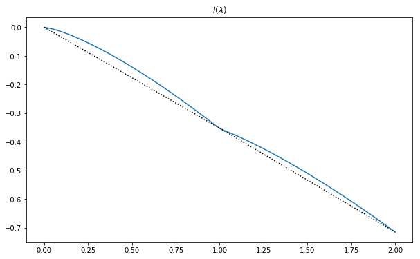
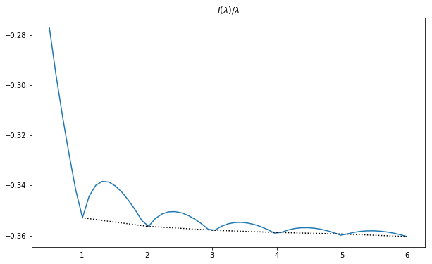
The concavity over is not expected to hold in general. Intuitively, for the derivative should be equal to the last (partially) filled eigenvalue (see (43) below for a one-sided estimate). However at we expect that whereas which respectively correspond to the last filled eigenvalue when we decrease the mass or to the next eigenvalue to be filled when we increase it. Since , is not expected to be concave except when .
A numerical computation in dimension in Figure 4 below confirms that is not concave over . Also is not decreasing, except when restricted to integers.
The next theorem follows from using the concentration-compactness technique for operators [Fri03, FLSS07, Lew11, LL10] and from the concavity of on each . It also follows from a profile decomposition similar to that used in [HKY19]. We will not write the proof in this paper, since the result is in fact also contained in [Lew11, Thm. 27] (with there) using Remark 8 about the link with the -particle problem.
Theorem 14 (Existence under the binding condition).
Let and . Let be such that the following binding inequalities hold:
| (37) |
Then, the problem has a minimiser.
In usual concentration compactness theory, one requires the continuous binding inequality
These inequalities automatically follow from the integer case (37) because the function is concave over each interval (Lemma 12), hence its minimum is attained either at or at .
Remark 15 (Non-integer case).
Let and be such that
By the concentration-compactness method one can conclude that has a minimiser. Note that is included in the above conditions.
2.3. Properties of minimisers
Here we state some general properties of minimisers, assuming they exist.
Proposition 16 (Euler-Lagrange equations).
Let and . If admits minimisers then it possesses one which is of the form in (33), with (orthonormal) real-valued eigenfunctions:
| (38) |
where is the smallest integer such that . The are the first eigenfunctions of the operator , counted with multiplicity:
| (39) |
with . In particular, has at least negative eigenvalues. The functions are real-analytic and tend to zero at infinity. Finally, we have the estimate
| (40) |
on the last filled eigenvalue.
Equation (38) can also be written in the compact operator form
where is a self-adjoint operator on , which is the sum of a projector plus a rank-one operator.
In the proof of the proposition, we are going to use the following remark which follows from the concavity of .
Lemma 17 (A general inequality).
Let and . Let and be two admissible operators. Then we have
| (41) |
where
is self-adjoint on and the trace in (41) is understood in the quadratic form sense.
Proof of Lemma 17.
The proof of (41) follows from the equality
and the fact that the last integrand is non-negative by the convexity of .
With Lemma 17 at hand we can write the
Proof of Proposition 16.
We split the proof into several steps.
Step 1: Equation.
Let be a minimiser for . Defining the complex conjugate which has the same density , we notice that
so we may assume that . The eigenfunctions of can then be chosen real.
Let be any other admissible operator of trace . Using (41) and the fact that we deduce that
In other words, also solves the linear minimisation problem
| (42) |
Minimisers of the linear problem (42) exist only when has at least non-positive eigenvalues, and are all of the form
with and . This is called the aufbau principle in quantum chemistry. The eigenvalues are filled starting from the bottom and only the last eigenvalue can be partially filled. Our minimiser must therefore be of this form. Note that is real since is a real function, therefore is real as well. We conclude that . It remains to show that is a projection plus a rank-one operator. In the next step we prove that , which already implies that must be finite rank.
Step 2: Estimates on .
We first show that . We consider , which is admissible for . From (41) we have22 2 This inequality also implies , see Remark 13.
| (43) |
Using and the explicit formula for in (6) we obtain the inequality
Next we derive the lower bound (40) on . To this end we use the virial (also called Pohozaev) identity. Let be the rescaled operator as in (35). Then the function
must attain its minimum at . Writing that the derivative vanishes at this point we find the virial identity
This gives
so that
| (44) |
where the last inequality comes from the fact that for all . We obtain as claimed
Step 3: Regularity and decay.
Note that the first eigenfunction of is always positive and non-degenerate. Therefore . Since we now have a system of finitely many coupled Partial Differential Equations, the real-analyticity of the ’s follows from classical results [Mor58, Kat96].
Next we show that the functions tend to 0 at infinity. In dimension , this follows from the fact that as we have seen in Lemma 17. In dimensions we need to employ a simple boot-strap argument. Assuming that for all , we infer that and then . When , the Sobolev embedding shows that with . This function has the two fixed points and , the latter being unstable. Starting from any we obtain after iterating finitely many times an . The Sobolev-Morrey embeddings now prove that the are continuous and tend to 0 at infinity.
Step 4. Form of
To prove that is a finite rank projection plus a rank-one operator, we assume by contradiction that has two eigenvalues with corresponding orthonormal real-valued eigenfunctions and we vary the corresponding eigenvalues linearly like , as we did in the proof of Lemma 11. The energy is concave in , hence must be constant since is a minimiser. The nonlinear term is even strictly concave, unless . Since these are real-analytic real-valued functions, it would imply everywhere, a contradiction. Therefore, at most one eigenvalue of can be in and this concludes the proof of Proposition 16. ∎
Remark 18.
The upper bounds on in (40) deteriorates when . We were not able to bound , as it probably requires the evaluation of , which may vanish as .
Using the Euler-Lagrange equation (39), we can prove that the functions (and therefore the density ) are exponentially decaying. Actually, we may provide lower bounds as well. This is not obvious, because the functions have non trivial nodal sets for . Only is positive everywhere. Following [BM77, HOHOS85], we introduce, for , the -spherical average
| (45) |
In the second integral we use the normalised Haar measure on SO.
Lemma 19 (Decay of minimisers at infinity).
The slowest exponential is the one corresponding to the th eigenvalue and it is the leading term in the density .
Proof of Lemma 19.
First we derive a non-optimal exponential bound on . We have
where we used the fact that in the last inequality. Since goes to at infinity and , there exists a large enough such that for all . In particular, we have
Let be the Yukawa potential, solution to on . Here is the modified Bessel function of the second kind. From the asymptotic behavior of [AS64, 9.7.2] we have
| (48) |
On the sphere of radius , the function is bounded, so we have for some with . Since
we deduce from the maximum principle [LL01, Chapter 9.4] that on . The function is bounded on and therefore we have proved the pointwise upper bound
| (49) |
Compared with (46), we see that a factor is missing in the exponential. However we have learned that the potential is exponentially decaying at infinity and for proving (47) we can now rely on existing results for the eigenfunctions of the linear Schrödinger operator .
The upper bound in (47) is well known but we give a detailed proof for completeness. Let for instance with which solves, this time,
| (50) |
see for instance [DR17]. We choose small enough so that the inverse-square potential is attractive: . In other words, we take in dimension and in dimension . The function is then positive on . In dimension we have to take and the resulting radial function vanishes infinitely many times close to the origin but it is positive for [FS70]. In all cases we have again
by [AS64, 9.7.2]. Using Kato’s inequality [RS75, Theorem X.27] and the exponential decay of we find
for large enough. The maximum principle then gives as before on , and thus the upper bound on in (47). For the estimate on , we can use that
with , so that
The function is integrable in a neighborhood of the origin and it behaves like at infinity, due to the fact that
| (51) |
see [AS64, 9.7.4]. Thus, using our bound on and the exponential bound (49) for , we find
with . The first term on the right behaves like at infinity, since is integrable and has compact support. For the second term we remark that the Fourier transform of is proportional to
and hence
| (52) |
The pointwise bound on in (47) follows from the behaviour (48) of at infinity and the fact that is , hence is bounded on compact sets.
2.4. Proof of binding
We now focus on the proof of the binding inequality . The usual proof is to consider minimisers for and , and to construct from them a good candidate for by putting these two minimisers far from each other. In our case, all quantities are exponentially decaying, which makes the evaluation of the interaction quite delicate. The following is the heart of the paper.
Proposition 20 (Exponentially small binding).
Let , and . Assume and admits the respective minimisers and , satisfying the properties in Proposition 16. Let and be the associated last filled eigenvalue of and . Then, under the additional condition
| (53) |
we have the binding inequality .
Proof.
We only write the proof in the integer case and for clarity. The arguments are exactly the same in the non-integer case, but the notation is a bit more heavy due to the additional rank-one operator.
Let and be two real minimisers for and respectively. Recall that our problem is invariant under rotations. Thus we can introduce and for some and deduce that these are minimisers of and as well. We will need to choose and appropriately. For clarity, we prefer to postpone this discussion to Lemma 21 below. Note that the functions satisfy the exponential bounds (47) uniformly in since those are invariant under rotations.
Next, we place the second system far away. For , we set where , and we introduce the Gram matrix
as we did in the proof of Lemma 12. Since the functions and are real-valued and exponentially decaying, is real and goes to exponentially fast. So the Gram matrix is real symmetric positive definite for large enough. As before, the frame
is orthonormal. Our trial state is the orthogonal projection onto this frame, given by
To compute , we consider the Taylor expansion with respect to the largest overlap
Note that . We compute all quantities to the order .
First, from , we have
This gives, to first order and with the translation of ,
| (54) |
where is the Sobolev-type trace norm. Let us evaluate the different terms in the energy. For the kinetic energy, we obtain (recall that everything is real-valued and that and are finite)
Using the Euler-Lagrange equations (8), we see that
with and . This gives for instance
Since is bounded, together with the definition of , we deduce that
We now compute the difference for the term . We first find an expression for , the density of . From (54), we get
This gives
Again, using that and are bounded functions, the last integral is of order . Altogether, this proves that
The orthonormalisation procedure generates an error of the order in the energy. The first term of the second line is the nonlinear interaction and it is always negative, from the concavity of . The question is whether it wins over the error term . This is the topic of the next result. We recall that our functions and depend on the two rotations and which we have introduced at the beginning of the proof and which we choose now, in terms of .
Lemma 21.
Let and and assume, without loss of generality, that . Then, there is so that for all large enough
| (55) |
uniformly in . On the other hand, for every large enough there exists such that
| (56) |
In particular, if , then .
The polynomial factors and in (55) and (56) are not necessarily optimal but will suffice for our argument. Before we provide the proof of Lemma 21, we remark that it immediately gives the strict inequality
after taking large enough, whenever . This condition is equivalent to the one in (53). It thus only remains to provide the proof of Lemma 21.
Proof of Lemma 21.
Let us first bound . By Lemma 19 we have and with and . Thus we find
When we have by (52). When we can use that which behaves at infinity like , by (51). This gives the bound (55).
Let us now bound from below. Recall that and From Lemma 19, the spherical average of is bounded below in terms of . This means that for any large enough , there exists at least one on the sphere of radius such that . The same lemma provides the pointwise upper bound and this implies that
on the ball with . The same property holds for at a point . We choose the rotations and to align the points and with the radii chosen to obtain the largest possible interaction. More precisely, we introduce the point
where and are of the same order . We then take such that
We obtain
for all , with
Since the function is increasing in and in separately for , we deduce that
for all . From the positivity of the integrand on we thus obtain
which is the claimed lower bound (56). ∎
This concludes the proof of Proposition 20. ∎
One immediate consequence of Proposition 20 is the case , where the condition (53) is always satisfied whenever . Since always has a minimiser, we also conclude that always has one, for .
Corollary 22.
Let and . Then, if has a minimiser, we have . In particular, and has a minimiser.
2.5. Proof of Theorem 3
Assume that and have minimisers. Let and be the corresponding last filled eigenvalues. From (40) in the integer case , and the fact that by (i) in Lemma 12, we have
| (57) |
Let be the first zero of the function
Using that and have a finite limit when we deduce that . Hence, if and have minimisers and if , then by Proposition 20.
Since we already know that has a minimiser, we can deduce by induction on that binding holds and that has a minimiser for all , when . This concludes the proof of Theorem 3.∎
Remark 23 (Numerical evaluation of ).
Any lower bound on and on the Lieb-Thirring constant appearing in the definition (24) of yields a lower bound on . The NLS energy can easily be computed numerically to a high precision since this amounts to solving an ordinary differential equation for the radial function . Using a Runge-Kunta solver for and the recent lower bound
| (58) |
from [FHJN19, Prop. 10] (see also [Fra20, Thm. 5]), we obtained the lower bounds mentioned in (13) for in dimensions . Should be equal to its conjectured value , we would obtain the slightly better bound .
2.6. Proof of Theorem 4
We now prove that has a minimiser for an infinity of integers . Let us call the set of all the integers which satisfies the binding inequalities for all . In particular, has a minimiser for all . For we already know that . Our goal is to show that is not finite.
If , then there is so that . If or , we can further decompose or , and so on, until we obtain a decomposition of the form
| (61) |
We claim that and prove this by contradiction. Let be so that in the previous decomposition. Then, since , we have by Proposition 20 that . Together with the weak-binding inequality, this would imply
In other words, if two of more ”bubbles” have the same number of particles, it is energetically favourable for these bubbles to merge. This gives
which is in contradiction with (61). So the coefficients in (61) must all be equal to or . Now cannot be finite otherwise we would not be able to write all the as in (61) with . This concludes the proof that is infinite. ∎
2.7. Proof of Theorem 10 on the large– limit
Using the Lieb-Thirring inequality (14), we have already seen in (i) in Lemma 12 that
In particular, we see that is bounded from below.
In Lemma 12 we have also shown in (ii) that for every integer . We deduce first that which appears in the upper bound (23). The first inequality is in fact strict when , by Corollary 22. Since the function is subadditive and bounded from below by a constant times we conclude that converges to its infimum as in (22), by Fekete’s subadditive lemma [Fek23].
It remains to prove the upper bound on in terms of the semi-classical constant . Instead of using the Dirichlet eigenfunctions of a large domain , as we mentioned after Theorem 10, we rather localise the periodic eigenfunctions in a cube (plane waves), which gives more explicit formulas. Let be the cube of side length centered at the origin and let be such that . Denote
for . It turns out that these functions are orthonormal, since
due to the fact that for . A computation gives that the kinetic energy of each such function is equal to
The second term is a since the function is equal to 1 inside , at a distance of order one to its boundary, and vanishes outside at a similar distance. We take such functions, each with a different , with given by (21) in Lemma 9 and . We find the energy
The first term is minimum when we take for the all the points of in a ball of fixed radius , where is chosen so that there are points, that is, . Taking the limit gives the upper bound in (23).∎
Using that is Lipschitz by (iii) in Lemma 12, we infer
for any . This proves that has the same limit as when it is restricted to integers:
| (62) |
Using similar arguments as in the proof of Theorem 4, we can then prove that is always strictly above its limit, independently of whether it admits a minimiser or not.
Corollary 24.
Let and . For all and all we have . In particular, we have
| (63) |
for all .
Proof.
If has a minimiser, this was already proved in Corollary 22. This covers in particular the case . If does not have a minimiser, then, according to Remark 15, there is an integer so that . By further decomposing , we can therefore write as in (61),
and at least one has value . So we have, as before
This concludes the proof of Corollary 24. ∎
3. Application: Symmetry breaking for a crystal in the Kohn-Sham model with large Dirac exchange
In this section we explain how the previous results can be used to prove symmetry breaking for an infinite periodic system, within a simple Kohn-Sham model with a Dirac (a.k.a. Slater) term. The results of this section are similar to a recent work by Ricaud [Ric18] on the Thomas-Fermi-von Weisäcker-Dirac model, so some technical details will be omitted for shortness. The main difference is that we deal with operators instead of functions. Our results can be generalised to other contexts, such as the symmetry breaking in the dissociation of the hydrogen molecule considered in [HHL+19].
3.1. Notation and main results
Everywhere in this section we fix the dimension . Let be a lattice of , with unit cell denoted by and dual lattice by . We consider the infinite system obtained by placing one point nucleus of charge at each site of this lattice,33 3 More generally we could place several nuclei of charges in each unit cell, so that the total charge is . together with an infinite sea of quantum electrons in a periodic state. We assume that the system is locally neutral, which means that the number of electrons per unit volume must be equal to . Our goal is to determine whether these electrons will have the same periodicity as the lattice of the nuclei or whether it is more favourable energetically to place them with a different period. In the latter case we say that there is spatial symmetry breaking. More specifically, we will study whether the -periodic electronic ground state is -periodic or not, for .
We recall that an -periodic density matrix is a self-adjoint operator on (we neglect the spin for simplicity) which commutes with all the translations of the lattice :
Here is the unitary operator on defined by . We restrict ourselves to density matrices which have a finite trace and a finite kinetic energy per unit volume, which means that and are locally trace-class. The density of is the unique -periodic function such that
for every of compact support. Any such density matrix represents an infinite periodic system of electrons. The number of electrons in each unit cell is defined by
In this section we work with electronic density matrices which are -periodic for some . All the previous definitions are easily extended to the case . Our main goal is to determine whether an -periodic minimiser is necessarily -periodic or not. In what follows, we enforce neutrality of the system. So, in any supercell of the type , we impose
The functional to minimise is the Kohn-Sham energy per unit cell which is defined by
| (64) |
for any -periodic density matrix . The first term is the kinetic energy per unit cell , interpreted in the sense of quadratic forms. The second term is the interaction between the -periodic electrons and the lattice of the nuclei of charge . The function is the -periodic Green’s function, solution to the periodic Laplace equation
| (65) |
In other words, is the Coulomb potential of the infinite lattice of nuclei, screened by a uniform background. The third term in (64) is the Coulomb interaction between the electrons in the Hartree approximation and it reads
where is defined similarly as in (65) with replaced by and replaced by . Finally, the last term of (64) is the Dirac or Slater term. This term is an approximation of the exchange-correlation energy of , in terms of the density only. The parameter usually has a fixed value given by physical considerations (for the exchange part of the energy the constant is without spin [LS10, Sec. 6.2]). Here, we change the value of , and compare the resulting energies for different values of the periodicity of the electrons.
The minimisation problem to be considered reads
| (66) |
The existence of minimisers easily follows from the direct method of the calculus of variations, since the problem is posed on the compact set [CLL01, CDL08a]. An -periodic state is of course -periodic and its Kohn-Sham energy is found to be equal to . In particular we deduce that
for every and every .
Definition 25 (Symmetry breaking).
We say that there is spatial symmetry breaking for the Dirac-Kohn-Sham model with parameter if there exists such that
The definition means that an -periodic minimiser has a lower energy per unit volume than the -periodic state. It does not mean that the electrons will necessarily be in this -periodic state. But at least we can deduce that they will not be -periodic.
The case is studied at length in [CLL01] and in [CDL08a, App. A]. In this situation the energy is convex and the problem admits a unique minimiser for every . This state solves the nonlinear equation
| (67) |
where is a Lagrange multiplier chosen to enforce the constraint that has electrons per unit cell. In addition, it is unique in the sense that any -periodic solution to equation (67) for some with the right number of electrons must be equal to . Since the -periodic state with is a solution for all , it follows that
and therefore that
No symmetry breaking occurs for . For latter purposes, we mention that the system is called an insulator when can be chosen in a spectral gap of the operator in (67) and that it is a metal otherwise. Which of the two cases occurs depends on the shape of the lattice and on the number of particles per unit cell.
The Dirac term is not convex when . It is natural to expect that symmetry will not be broken for small enough whereas it could be broken for large . This is confirmed by the following result.
Theorem 26 (Occurrence of symmetry breaking).
Let be a lattice in and . There is a critical such that, for all , the system breaks spatial symmetry. In addition, if the system is insulating at , then : there exists such that for all and all .
The spirit of the result is exactly the same as [Ric18] in the Thomas-Fermi-von Weisäcker-Dirac case. For very large the kinetic energy and the Dirac term dominate, the other terms being of lower order. The very large constant has the effect of concentrating the electrons at the scale . After rescaling length by a factor about a blow-up point, in the limit the problem converges to the fermionic NLS problem in the whole space with . This is the content of the following result.
Proposition 27 (Convergence to the NLS problem in ).
In Theorem 4 and in Corollary 24 we have proved that for all . This shows that for large enough , hence that there is symmetry breaking. The intuitive picture is that it is more favourable to concentrate particles at one point rather than having bumps of concentrated electrons, as is the case for the -periodic minimiser placed in the -periodic energy. This is how we can prove the first part of Theorem 26.
Remark 28.
The previous result does not use that . However, since this inequality has been numerically found to hold (see Remark 23), minimisers for always exist, and one can say more. Following the approach of [Ric18], it is possible to prove that minimisers for satisfy weakly- locally in the trace class, where minimises and is the dilation operator defined by . In other words, the electrons concentrate at the origin where the nucleus is placed, in the unit cell . For the result is similar but the electrons concentrate at one of the nuclei of the larger unit cell . Finally, we have the expansion
The literature contains several results in the same spirit as Theorem 26 and Proposition 27. The closest to our work is [HHL+19] which studies the case of the Kohn-Sham hydrogen molecule (two electrons in the field of two nuclei separated by a distance ). This corresponds to but since the spin is taken into account there is no orthogonality constraint between and . In this model, spin symmetry breaking arises in the limit because each electron has to concentrate about one of the two nuclei, where it asymptotically solves the NLS problem . This is therefore a completely different phenomenon from this present work, where the two particles concentrate at the same point. Other works in the same spirit include for instance [AFG+02, GS14, GZZ16] for the Hartree model in multiple well potentials, which also has no orthogonality constraint.
3.2. Sketch of the proof of Proposition 27 and of the first part of Theorem 26
The symmetry breaking stated in the first part of Theorem 26 follows immediately from Proposition 27, the proof of which we outline in this section.
We set for simplicity (the proof is similar in the general case). For an -periodic density matrix, we call the rescaled operator whose kernel is
| (68) |
Using that , we obtain the following scaling relations:
We deduce that the energy of can be re-expressed as
| (69) |
with
The energy is similar to the NLS energy in (31) except that the problem is restricted to the flat torus of size , instead of being posed over the whole of .
Step 1.
Let us first prove that
| (70) |
Let be a smooth rank- projector of compact support such that44 4 To obtain such a one can start with a trial state and then truncate and regularise the ’s. The new functions can be orthonormalised using the same procedure as in Lemma 12. . This state can be used as a trial state in the rescaled box , as soon as its support is strictly included in . This amounts to -periodising in the manner . Then whereas
Hence
The claimed bound (70) follows after taking and then .
Step 2.
To prove the other inequality
| (71) |
we consider a minimiser for and call the rescaled operator as in (68). From the previous step and the positivity of the Hartree term, we have for large enough
| (72) |
Using the Gagliardo-Nirenberg and Hoffmann-Ostenhof periodic inequalities, we have
Similarly, to control the potential energy, we use that , and obtain by Hardy’s inequality
Inserting in (72) this gives and hence after scaling we obtain
This gives
The last step is to show that
| (73) |
To prove (73) we decompose into bubbles. We use the operator version of the bubble decomposition, which has implicitly appeared several times in the literature and can be read with full details in the recent work [HKY19, Theorem 3.1]. The present setting is slightly different from [HKY19] due to the periodic boundary condition but the proof is similar, see, e.g., [Ric18] in the case of functions. For operators the result is that there exists a sequence of density matrices over with such that
and
The Dirac term decomposes exactly since is a sub-critical power, whereas for the mass and the kinetic energy one only obtains lower bounds. The missing mass and kinetic energy are contained in the vanishing part of , to employ the vocabulary of the concentration-compactness method. Each is constructed as the strong local limit of for some translation and some localisation function , with when , up to subsequences. Using the subadditivity of proved in Lemma 12, we deduce that
| (74) |
This concludes our sketch of the proof of Proposition 27.∎
3.3. Proof of the second point of Theorem 26: stability for small
When , we have recalled from [CDL08a, App. A] that the minimisation problem admits a unique minimiser, which we denote here by (it was called above). It solves the nonlinear operator equation
| (75) |
where is a Lagrange multiplier and
The assumption that the system is an insulator means that belongs to a spectral gap of the operator . For simplicity, we denote by
and, without loss of generality, we can choose
The length of the gap is . Let us prove that . After a Bloch-Floquet transform [RS78], the equation (75) means that the kernel of is given by
with the density
Here is the Brillouin zone (the unit cell of the dual lattice ) and are the Bloch eigenfunctions and (ordered) eigenvalues, which solve
with periodic boundary conditions on . By Perron-Frobenius we have and . By perturbation theory we then deduce that is non-degenerate with a positive eigenfunction , for small enough. Then and in the following we denote by
the minimal value of the periodic density.
The following shows that the gap does not close and the density stays strictly positive for small enough.
Lemma 29 (Stability of the gap).
There is such that, for all , any minimiser for satisfies
where we set , and
Finally, we have and there is independent of so that the following operator inequality holds:
| (76) |
Proof.
Let . The energy is continuous at and any minimiser is a minimising sequence for . Hence it must converge to the unique minimiser weakly and
This implies that strongly in . Then we write the associated mean-field operator in the form
and estimate the operator norms of the last two terms by
and
With similar estimates we know that and are bounded for large enough, locally uniformly in , see [CDL08a, Lem. 1]. By the Rellich-Kato theorem, this proves that the spectrum of converges to that of . In particular, has a gap around , independent of for small enough. To conclude we have therefore shown that there exists so that any minimiser for has a mean-field operator with the gap around . This implies (76) by [CDL08a, Lem. 3].
Let then be any such minimiser for . Since the family has a gap for all and the rank of a continuous family of orthogonal projectors is always constant, we obtain
By [CDL08a, App. A] we know that where is the unique Lagrange multiplier chosen such that , and we conclude that is independent of . In particular .
Finally, we have
Since and are bounded, this shows that uniformly in . This implies that is bounded in and therefore we have in when . In particular for small enough. ∎
Next we use the properties of minimisers for in Lemma 29 to show that there is indeed only one, for every .
Lemma 30.
There is so that, for all , has a unique minimiser , satisfying the properties of Lemma 29. This minimiser is also the unique minimiser for for all , hence there is no symmetry breaking for .
Proof.
We use the framework developed in [BBHS99, HLS05, CDL08a, CDL08b, FLLS12]. Let be any minimiser for with and let be any other -periodic density matrix. Using , we can rewrite and estimate the difference of the two energies as
| (77) |
where . In the second line we have used that
for all and that . Our goal is to show that (77) is non-negative and vanishes only at . We claim that
| (78) |
The result then follows under the assumption that .
To prove (78) we introduce
and note that
We have used Bach’s inequality from [BBHS99, Eq. (18)–(19)].
For we use the Lieb-Thirring inequality which implies
and provides the desired bound on the two densities and .
For and the argument is slightly more involved. Following [CDL08a, Prop. 1] we claim that
| (79) |
where the constant is independent of . The argument goes by duality in the form
with the Hilbert-Schmidt norm on a Hilbert space . We have
for a constant independent of . We obtain an upper bound involving
We compute this Hilbert-Schmidt norm in the Fourier basis , which gives
This concludes our sketch of the proof of (79), hence of (78) and of Theorem 26. ∎
Acknowledgement
This project has received funding from the European Research Council (ERC) under the European Union’s Horizon 2020 research and innovation programme (grant agreement MDFT 725528 of M.L.).
References
- [AC06] A. Ambrosetti and E. Colorado, Bound and ground states of coupled nonlinear Schrödinger equations, C. R. Math. Acad. Sci. Paris, 342 (2006), pp. 453–458.
- [AFG+02] W. Aschbacher, J. Fröhlich, G. Graf, K. Schnee, and M. Troyer, Symmetry breaking regime in the nonlinear Hartree equation, J. Math. Phys., 43 (2002), pp. 3879–3891.
- [Alb88] C. Albanese, Localised solutions of Hartree equations for narrow-band crystals, Comm. Math. Phys., 120 (1988), pp. 97–103.
- [AS64] M. Abramowitz and I. A. Stegun, Handbook of mathematical functions with formulas, graphs, and mathematical tables, vol. 55 of National Bureau of Standards Applied Mathematics Series, For sale by the Superintendent of Documents, U.S. Government Printing Office, Washington, D.C., 1964.
- [Bac92] V. Bach, Error bound for the Hartree-Fock energy of atoms and molecules, Commun. Math. Phys., 147 (1992), pp. 527–548.
- [Bac93] , Accuracy of mean field approximations for atoms and molecules, Comm. Math. Phys., 155 (1993), pp. 295–310.
- [BBHS99] V. Bach, J. M. Barbaroux, B. Helffer, and H. Siedentop, On the stability of the relativistic electron-positron field, Commun. Math. Phys., 201 (1999), pp. 445–460.
- [BHL+17] N. Bez, Y. Hong, S. Lee, S. Nakamura, and Y. Sawano, On the Strichartz estimates for orthonormal systems of initial data with regularity, ArXiv e-prints, (2017).
- [BL83] H. Berestycki and P.-L. Lions, Nonlinear scalar field equations. I. Existence of a ground state, Arch. Rational Mech. Anal., 82 (1983), pp. 313–345.
- [BL90] A. Bahri and Y. Y. Li, On a min-max procedure for the existence of a positive solution for certain scalar field equations in , Rev. Mat. Iberoamericana, 6 (1990), pp. 1–15.
- [BL97] A. Bahri and P.-L. Lions, On the existence of a positive solution of semilinear elliptic equations in unbounded domains, Ann. Inst. H. Poincaré Anal. Non Linéaire, 14 (1997), pp. 365–413.
- [BL15] X. Blanc and M. Lewin, The crystallization conjecture: A review, EMS Surv. Math. Sci., 2 (2015), pp. 219–306.
- [BLLS94] V. Bach, E. H. Lieb, M. Loss, and J. P. Solovej, There are no unfilled shells in unrestricted Hartree-Fock theory, Phys. Rev. Lett., 72 (1994), pp. 2981–2983.
- [BLS94] V. Bach, E. H. Lieb, and J. P. Solovej, Generalized Hartree-Fock theory and the Hubbard model, J. Statist. Phys., 76 (1994), pp. 3–89.
- [BM77] C. Bardos and M. Merigot, Asymptotic decay of the solution of a second-order elliptic equation in an unbounded domain. applications to the spectral properties of a hamiltonian, Proc. R. Soc. Edinburgh A, 76 (1977), pp. 323–344.
- [BW06] T. Bartsch and Z.-Q. Wang, Note on ground states of nonlinear Schrödinger systems, J. Partial Differential Equations, 19 (2006), pp. 200–207.
- [BWW07] T. Bartsch, Z.-Q. Wang, and J. Wei, Bound states for a coupled Schrödinger system, J. Fixed Point Theory Appl., 2 (2007), pp. 353–367.
- [Cd18] C. Collot and A.-S. de Suzzoni, Stability of equilibria for a Hartree equation for random fields, arXiv e-prints, (2018), p. arXiv:1811.03150.
- [CDL08a] É. Cancès, A. Deleurence, and M. Lewin, A new approach to the modelling of local defects in crystals: the reduced Hartree-Fock case, Commun. Math. Phys., 281 (2008), pp. 129–177.
- [CDL08b] , Non-perturbative embedding of local defects in crystalline materials, J. Phys.: Condens. Matter, 20 (2008), p. 294213.
- [CHP17a] T. Chen, Y. Hong, and N. Pavlović, Global Well-Posedness of the NLS System for Infinitely Many Fermions, Archive for Rational Mechanics and Analysis, 224 (2017), pp. 91–123.
- [CHP17b] , On the scattering problem for infinitely many fermions in dimensions at positive temperature, Annales de l’Institut Henri Poincaré (C) Non Linear Analysis, (2017).
- [CL92] I. Catto and P.-L. Lions, Binding of atoms and stability of molecules in Hartree and Thomas-Fermi type theories. I. A necessary and sufficient condition for the stability of general molecular systems, Comm. Partial Differential Equations, 17 (1992), pp. 1051–1110.
- [CL93a] , Binding of atoms and stability of molecules in Hartree and Thomas-Fermi type theories. II. Stability is equivalent to the binding of neutral subsystems, Comm. Partial Differential Equations, 18 (1993), pp. 305–354.
- [CL93b] , Binding of atoms and stability of molecules in Hartree and Thomas-Fermi type theories. III. Binding of neutral subsystems, Comm. Partial Differential Equations, 18 (1993), pp. 381–429.
- [CLL01] I. Catto, C. Le Bris, and P.-L. Lions, On the thermodynamic limit for Hartree-Fock type models, Ann. Inst. H. Poincaré Anal. Non Linéaire, 18 (2001), pp. 687–760.
- [Cof72] C. V. Coffman, Uniqueness of the ground state solution for and a variational characterization of other solutions, Arch. Rational Mech. Anal., 46 (1972), pp. 81–95.
- [Dau94] F. Daumer, Équations de Hartree-Fock dans l’approximation du tight-binding, Helv. Phys. Acta, 67 (1994), pp. 237–256.
- [de 15] A.-S. de Suzzoni, An equation on random variables and systems of fermions, arXiv e-prints, (2015).
- [DR17] J. Dereziński and S. Richard, On Schrödinger operators with inverse square potentials on the half-line, Ann. Henri Poincaré, 18 (2017), pp. 869–928.
- [Fek23] M. Fekete, Über die Verteilung der Wurzeln bei gewissen algebraischen Gleichungen mit ganzzahligen Koeffizienten, Math. Z., 17 (1923), pp. 228–249.
- [FGL20a] R. L. Frank, D. Gontier, and M. Lewin, The nonlinear Schrödinger equation for orthonormal functions II. Application to Lieb-Thirring inequalities, Comm. Math. Phys., in press (2020).
- [FGL20b] , The periodic Lieb–Thirring inequality, ArXiV e-prints, (2020). To Ari Laptev on the occasion of his 70th birthday.
- [FHJN19] R. L. Frank, D. Hundertmark, M. Jex, and P. T. Nam, The Lieb-Thirring inequality revisited, J. Eur. Math. Soc. (JEMS), in press (2019), p. arXiv:1808.09017.
- [FI73] B. D. Fried and Y. H. Ichikawa, On the Nonlinear Schrödinger Equation for Langmuir Waves, J. Phys. Soc. Jpn., 34 (1973), pp. 1073–1082.
- [FLLS12] R. L. Frank, M. Lewin, E. H. Lieb, and R. Seiringer, A positive density analogue of the Lieb-Thirring inequality, Duke Math. J., 162 (2012), pp. 435–495.
- [FLLS14] , Strichartz inequality for orthonormal functions, J. Eur. Math. Soc. (JEMS), 16 (2014), pp. 1507–1526.
- [FLSS07] R. L. Frank, E. H. Lieb, R. Seiringer, and H. Siedentop, Müller’s exchange-correlation energy in density-matrix-functional theory, Phys. Rev. A, 76 (2007), p. 052517.
- [Fra13] R. L. Frank, Ground states of semi-linear PDE. Lecture notes from the “Summerschool on Current Topics in Mathematical Physics”, CIRM Marseille, Sept. 2013., 2013.
- [Fra20] , The Lieb–Thirring inequality: Recent results and open problems, arXiv:2007.09326, (2020).
- [Fri03] G. Friesecke, The multiconfiguration equations for atoms and molecules: charge quantization and existence of solutions, Arch. Ration. Mech. Anal., 169 (2003), pp. 35–71.
- [FS70] E. M. Ferreira and J. Sesma, Zeros of the modified Hankel function, Numer. Math., 16 (1970), pp. 278–284.
- [FS17] R. L. Frank and J. Sabin, Restriction theorems for orthonormal functions, Strichartz inequalities, and uniform Sobolev estimates, Amer. Math. J., 139 (2017), pp. 1649–1691.
- [GS14] Y. Guo and R. Seiringer, On the mass concentration for Bose-Einstein condensates with attractive interactions, Lett. Math. Phys., 104 (2014), pp. 141–156.
- [GZZ16] Y. Guo, X. Zeng, and H.-S. Zhou, Energy estimates and symmetry breaking in attractive Bose-Einstein condensates with ring-shaped potentials, Ann. Inst. H. Poincaré Anal. Non Linéaire, 33 (2016), pp. 809–828.
- [HH77] M. Hoffmann-Ostenhof and T. Hoffmann-Ostenhof, Schrödinger inequalities and asymptotic behavior of the electron density of atoms and molecules, Phys. Rev. A, 16 (1977), pp. 1782–1785.
- [HHL+19] M. Holst, H. Hu, J. Lu, J. Marzuola, D. Song, and J. Weare, Symmetry Breaking in Density Functional Theory due to Dirac Exchange for a Hydrogen Molecule. Preprint arXiv:1902.03497, 2019.
- [HKY19] Y. Hong, S. Kwon, and H. Yoon, Global existence versus finite time blowup dichotomy for the system of nonlinear Schrödinger equations, J. Math. Pures Appl., 125 (2019), pp. 283–320.
- [HLS05] C. Hainzl, M. Lewin, and É. Séré, Existence of a stable polarized vacuum in the Bogoliubov-Dirac-Fock approximation, Commun. Math. Phys., 257 (2005), pp. 515–562.
- [HOHOS85] M. Hoffmann-Ostenhof, T. Hoffmann-Ostenhof, and J. Swetina, Pointwise bounds on the asymptotics of spherically averaged -solutions of one-body Schrödinger equations, Ann. IHP A, 42 (1985), pp. 341–361.
- [Kat96] K. Kato, New idea for proof of analyticity of solutions to analytic nonlinear elliptic equations, SUT J. Math., 32 (1996), pp. 157–161.
- [KF16] P. Kevrekidis and D. Frantzeskakis, Solitons in coupled nonlinear Schrödinger models: A survey of recent developments, Reviews in Physics, 1 (2016), pp. 140 – 153.
- [Kwo89] M. K. Kwong, Uniqueness of positive solutions of in , Arch. Rational Mech. Anal., 105 (1989), pp. 243–266.
- [Lew10] M. Lewin, Describing lack of compactness in Sobolev spaces. Variational Methods in Quantum Mechanics, unpublished lecture notes for a Master course given at the University of Cergy-Pontoise, hal:02450559, 2010.
- [Lew11] , Geometric methods for nonlinear many-body quantum systems, J. Funct. Anal., 260 (2011), pp. 3535–3595.
- [Lie81] E. H. Lieb, Variational principle for many-fermion systems, Phys. Rev. Lett., 46 (1981), pp. 457–459.
- [Lie83a] , Density functionals for Coulomb systems, Int. J. Quantum Chem., 24 (1983), pp. 243–277.
- [Lie83b] , An bound for the Riesz and Bessel potentials of orthonormal functions, J. Funct. Anal., 51 (1983), pp. 159–165.
- [Lio82] P.-L. Lions, Principe de concentration-compacité en calcul des variations, C. R. Acad. Sci. Paris Sér. I Math., 294 (1982), pp. 261–264.
- [Lio84a] , The concentration-compactness principle in the calculus of variations. The locally compact case, Part I, Ann. Inst. H. Poincaré Anal. Non Linéaire, 1 (1984), pp. 109–149.
- [Lio84b] , The concentration-compactness principle in the calculus of variations. The locally compact case, Part II, Ann. Inst. H. Poincaré Anal. Non Linéaire, 1 (1984), pp. 223–283.
- [LL01] E. H. Lieb and M. Loss, Analysis, vol. 14 of Graduate Studies in Mathematics, American Mathematical Society, Providence, RI, 2nd ed., 2001.
- [LL10] E. Lenzmann and M. Lewin, Minimizers for the Hartree-Fock-Bogoliubov theory of neutron stars and white dwarfs, Duke Math. J., 152 (2010), pp. 257–315.
- [LS10] E. H. Lieb and R. Seiringer, The Stability of Matter in Quantum Mechanics, Cambridge Univ. Press, 2010.
- [LS14] M. Lewin and J. Sabin, The Hartree equation for infinitely many particles. II. Dispersion and scattering in 2D, Analysis & PDE, 7 (2014), pp. 1339–1363.
- [LS15] , The Hartree equation for infinitely many particles. I. Well-posedness theory, Comm. Math. Phys., 334 (2015), pp. 117–170.
- [LSSY05] E. H. Lieb, R. Seiringer, J. P. Solovej, and J. Yngvason, The mathematics of the Bose gas and its condensation, Oberwolfach Seminars, Birkhäuser, 2005.
- [LT75] E. H. Lieb and W. E. Thirring, Bound on kinetic energy of fermions which proves stability of matter, Phys. Rev. Lett., 35 (1975), pp. 687–689.
- [LT76] , Inequalities for the moments of the eigenvalues of the Schrödinger hamiltonian and their relation to Sobolev inequalities, Studies in Mathematical Physics, Princeton University Press, 1976, pp. 269–303.
- [LW05] T.-C. Lin and J. Wei, Ground state of coupled nonlinear Schrödinger equations in , , Comm. Math. Phys., 255 (2005), pp. 629–653.
- [Mal05] B. Malomed, Encyclopedia of Nonlinear Science, Routledge, 2005, ch. Nonlinear Schrödinger Equations, pp. 639–642.
- [Man74] S. V. Manakov, On the theory of two-dimensional stationary self-focusing of electromagnetic waves, Soviet Phys. JETP, 38 (1974), pp. 505–516.
- [McL93] K. McLeod, Uniqueness of positive radial solutions of in . II, Trans. Amer. Math. Soc., 339 (1993), pp. 495–505.
- [Mor58] J. C. B. Morrey, On the analyticity of the solutions of analytic non-linear elliptic systems of partial differential equations. I. Analyticity in the interior., Amer. J. Math., 80 (1958), pp. 198–218.
- [OR20] A. Olgiati and N. Rougerie, The hartree functional in a double well, 2020.
- [Poh65] S. I. Pohozaev, On the eigenfunctions of the equation , Dokl. Akad. Nauk SSSR, 165 (1965), pp. 36–39.
- [PS03] L. P. Pitaevskii and S. Stringari, Bose-Einstein condensation, no. 116, Oxford University Press, 2003.
- [Ric18] J. Ricaud, Symmetry breaking in the periodic Thomas-Fermi-Dirac–von Weizsäcker model, Ann. Henri Poincaré, 19 (2018), pp. 3129–3177.
- [RS75] M. Reed and B. Simon, Methods of Modern Mathematical Physics. II. Fourier analysis, self-adjointness, Academic Press, New York, 1975.
- [RS78] , Methods of Modern Mathematical Physics. IV. Analysis of operators, Academic Press, New York, 1978.
- [Rue99] D. Ruelle, Statistical mechanics. Rigorous results, Singapore: World Scientific. London: Imperial College Press , 1999.
- [Sol91] J. P. Solovej, Proof of the ionization conjecture in a reduced Hartree-Fock model, Invent. Math., 104 (1991), pp. 291–311.
- [Tao06] T. Tao, Nonlinear dispersive equations, vol. 106 of CBMS Regional Conference Series in Mathematics, Published for the Conference Board of the Mathematical Sciences, Washington, DC, 2006. Local and global analysis.
- [TY69] T. Taniuti and N. Yajima, Perturbation method for a nonlinear wave modulation. I, J. Mathematical Phys., 10 (1969), pp. 1369–1372.
- [Wei83] M. I. Weinstein, Nonlinear Schrödinger equations and sharp interpolation estimates, Comm. Math. Phys., 87 (1983), pp. 567–576.
- [Wei85] , Modulational stability of ground states of nonlinear Schrödinger equations, SIAM J. Math. Anal., 16 (1985), pp. 472–491.
- [Zak68] V. E. Zakharov, Stability of periodic waves of finite amplitude on the surface of a deep fluid, J. Appl. Mech. Tech. Phys., 9 (1968), pp. 190–194.
- [ZS72] V. E. Zakharov and A. B. Shabat, Exact Theory of Two-dimensional Self-focusing and One-dimensional Self-modulation of Waves in Nonlinear Media, Soviet Phys. JETP, 34 (1972), p. 62.
- [ZY18] G. Zhang and Z. Yan, The -component nonlinear Schrödinger equations: dark-bright mixed - and high-order solitons and breathers, and dynamics, Proc. R. Soc. Lond. A, 474 (2018), p. 20170688.