Spatial-segregation limit for exclusion processes with two components under unbalanced reaction

Let $\mathbb{T}^{d}_{N}\cong\{1,...,N\}^{d}$ be the $d$-dimensional discrete torus and let $\mathcal{X}^{2}_{N}=\{0,1\}^{\mathbb{T}^{d}_{N}}\times\{0,1\}^{\mathbb{T}^{d}_{N}}$ be the configuration space of two kinds of particles. We denote an element $\eta=(\eta_{1},\eta_{2})\in\mathcal{X}^{2}_{N}$ with $\eta_{i}=\{\eta_{i}(x)\}_{x\in\mathbb{T}^{d}_{N}}$ $(i=1,2)$. Here for each $i=1,2$, an element $\eta_{i}$ represents the configuration of type-$i$ particles: $\eta_{i}(x)=1$ means there exists a type-$i$ particle on site $x\in\mathbb{T}^{d}_{N}$ and $\eta_{i}(x)=0$ means type-$i$ particle does not exist on site $x$. Next, we consider a kind of Glauber-Kawasaki processes which takes values on $\mathcal{X}^{2}_{N}$ as follows. We consider the simple exclusion process where only type-$1$ particles diffuse and its generator is given by

for each function $f:\mathcal{X}^{2}_{N}\to\mathbb{R}$. Here, for each $\sigma\in\mathcal{X}_{N}$, $\sigma^{x,y}$ is the configuration after exchanging occupation variables on sites $x$ and $y$:

On the other hand, the generator of the Glauber dynamics is given by $L_{G}=L_{1,G}+L_{2,G}$ with

for each function $f:\mathcal{X}^{2}_{N}\to\mathbb{R}$ where for each $\sigma\in\mathcal{X}_{N}$, $\sigma^{x}$ is the configuration after flipping the particle configuration on site $x$:

Here, $c_{i,x}(\eta_{1},\eta_{2})=c_{i}(\tau_{x}\eta_{1},\tau_{x}\eta_{2})$ for $i=1,2$ and $\{\tau_{x}\}_{x\in\mathbb{Z}^{d}}$ are shifts acting on $\mathcal{X}_{N}$ as $\tau_{x}\sigma(\cdot)=\sigma(\cdot+x)$ for every $\sigma\in\mathcal{X}_{N}$. Throughout this article, we assume that both annihilation rates $c_{i}(\eta_{1},\eta_{2})(i=1,2)$ are non-negative and depend only on the particle configuration of finite number of sites which depend neither on $\eta_{1}(0)$ nor $\eta_{2}(0)$ as follows:

and

with some real constants $c_{1,\Lambda_{1},\Lambda_{2}}$ and $c_{2,\Lambda}$ such that $c_{1}$ and $c_{2}$ stay non-negative and these constants are assumed to be zero except for finite numbers of them so that the above summation becomes finite. In this paper, we assume the reaction rate $c_{2}$ does not depend on configuration of type-$2$ particles. A technical reason for this assumption will be explained in the proof of the probabilistic part of main theorems given in Section 3 (see Remark 4.1). Moreover, for the sake of convenience described later we extend $c_{1}$ and $c_{2}$ as non-negative functionals on $[0,1]^{\mathbb{T}^{d}_{N}}\times[0,1]^{\mathbb{T}^{d}_{N}}$ by

and

for $(u,v)\in[0,1]^{\mathbb{T}^{d}_{N}}\times[0,1]^{\mathbb{T}^{d}_{N}}$ with $u=\{u(x)\}_{x\in\mathbb{T}^{d}_{N}}$ and $v=\{v(x)\}_{x\in\mathbb{T}^{d}_{N}}$. In other words, $c_{i}(u,v)$ is obtained by substituting $u(x)$ and $v(x)$ into $\eta_{1}(x)$ and $\eta_{2}(x)$, respectively, in the definition of $c_{1}(\eta_{1},\eta_{2})$ and $c_{2}(\eta_{1},\eta_{2})$ for every $x\in\mathbb{T}^{d}_{N}$.

For each $N\in\mathbb{N}$, let $\{\eta^{N}_{t}=(\eta^{N}_{1,t},\eta^{N}_{2,t})\}_{t\geq 0}$ be the $\mathcal{X}^{2}_{N}$-valued Markov process generated by $L_{N}=N^{2}L_{K}+K(N)L_{G}$ on some probability space $(\Omega_{N},\mathcal{F}_{N},\mathbb{P}^{N}_{\mu^{N}_{0}})$. Here for a probability measure $\mu$ on the configuration space $\mathcal{X}^{2}_{N}$, $\mathbb{P}^{N}_{\mu}$ is the probability measure under which the initial distribution of $\{\eta^{N}_{t}\}_{t\geq 0}$ is $\mu$ and we denote the expectation with respect to $\mathbb{P}^{N}_{\mu}$ by $\mathbb{E}^{N}_{\mu}[\cdot]$. An assumption for the initial distribution $\mu^{N}_{0}$ will be described later (see assumption (A2)). Here $K=K(N)$ is a divergent parameter as $N$ tends to infinity, which corresponds to take so-called “fast-reaction limit” in PDE context. Define macroscopic empirical measures $\{\pi^{N}_{t}=(\pi^{N}_{1,t},\pi^{N}_{2,t})\}_{t\geq 0}$ on the $d$-dimensional torus $\mathbb{T}^{d}\cong[0,1)^{d}$ by

and hereafter we write $\langle\pi^{N}_{i,t},\varphi\rangle:=\int_{\mathbb{T}^{d}}\varphi(\theta)\pi^{N}_{i,t}(d\theta)$ for any continuous function $\varphi$ on $\mathbb{T}^{d}$. Moreover, for any $\mathbb{R}^{2}$-valued continuous function $\varphi=(\varphi_{1},\varphi_{2})$, we denote its vector-valued integral by $\langle\pi^{N}_{t},\varphi\rangle\coloneqq(\langle\pi^{N}_{1,t},\varphi_{1}\rangle,\langle\pi^{N}_{2,t},\varphi_{2}\rangle)$.

Our aim is to study the limiting behavior of spatial density profiles of both kinds of particles under dynamics such that diffusion of type-$1$ particles is speeded up by $N^{2}$ and two species compete with rate $K(N)$ which diverges as $N$ tends to infinity. Particularly, we will show that for special forms of reaction rates $c_{i}$ $(i=1,2)$ (that is, Case 1, Case 2 and Case 3 which are described later) there are three regimes of interface growth.

To evaluate the difference between two probability measures, we use the relative entropy defined as follows. Let $\mu$ and $\nu$ be two probability measures on $\mathcal{X}^{2}_{N}$. We define the relative entropy of $\mu$ with respect to $\nu$ by

if $\mu$ is absolutely continuous with respect to $\nu$, while otherwise we define $H(\mu|\nu):=\infty$.

Next we summarize our assumptions on the initial distribution and state main theorems in this paper.

(A1):

Let $u^{N}(0,x)=u^{N}_{0}(x)$ and $v^{N}(0,x)=v^{N}_{0}(x)$ be given and satisfy two bounds

		$\displaystyle e^{-C_{1}K}\leq u^{N}(0,x)\leq C_{2},\quad|\nabla^{N}u^{N}(0,x)|\leq C_{0}K$
		$\displaystyle e^{-C_{1}K}\leq v^{N}(0,x)\leq C_{2},\quad|\nabla^{N}v^{N}(0,x)|\leq C_{0}K$

for every $x\in\mathbb{T}^{d}_{N}$ with $C_{1}>0$, $0<C_{2}<1$ and $C_{0}>0$. Here $\nabla^{N}$ is the discrete gradient, that is, for every $u:\mathbb{T}^{d}_{N}\to\mathbb{R}$ we define $\nabla^{N}u:\mathbb{T}^{d}_{N}\to\mathbb{R}^{d}$ by $\nabla^{N}u(x)=\left(N(u(x+e_{j})-u(x))\right)_{j=1,...,d}$.

(A2):

We denote $\mu^{N}_{0}$ the distribution of $\eta^{N}_{0}=(\eta^{N}_{1,0},\eta^{N}_{2,0})$ on $\mathcal{X}^{2}_{N}$ and let $\nu^{N}_{0}$ be the product Bernoulli measure on $\mathcal{X}^{2}_{N}$ with mean $(u^{N}(0,\cdot),v^{N}(0,\cdot))$. We assume the relative entropy $H(\mu^{N}_{0}|\nu^{N}_{0})$ defined by (2.1) satisfies $H(\mu^{N}_{0}|\nu^{N}_{0})=O(N^{d-{\delta_{0}}})$ for some $\delta_{0}>0$ as $N$ tends to infinity, that is, there exists a positive constant $M$ such that $H(\mu^{N}_{0}|\nu^{N}_{0})\leq MN^{d-{\delta_{0}}}$ for sufficiently large $N$.

(A3)_δ:

$K=K(N)$ satisfies $1\leq K(N)\leq\delta(\log N)^{1/2}$ and $K(N)\to\infty$ as $N$ tends to infinity.

For each $m\in\mathbb{N}$ and for some fixed sites $z_{i}\in\mathbb{Z}^{d}$ ($i=1,...,m-1$), we introduce the following three regimes which are special cases in our setting.

Case 1.:

$c_{1}(\eta_{1},\eta_{2})=\eta_{1}(z_{1})\cdots\eta_{1}(z_{m-1})$, $c_{2}(\eta_{1},\eta_{2})\equiv 1$ with $m>3$.

Case 2.:

$c_{1}(\eta_{1},\eta_{2})=\eta_{2}(z_{1})\cdots\eta_{2}(z_{m-1})$, $c_{2}(\eta_{1},\eta_{2})\equiv 1$ with $m\geq 1$.

Case 3.:

$c_{1}(\eta_{1},\eta_{2})\equiv 1$, $c_{2}(\eta_{1},\eta_{2})=\eta_{1}(z_{1})\cdots\eta_{1}(z_{m-1})$ with $m>1$.

Here we suppose $c_{1}\equiv 1$ when $m=1$ in Case 2 and $c_{2}\equiv 1$ when $m=1$ in Case 3 by convention. For each regime, we have the following hydrodynamic limit result which describes the limiting behavior of interfaces between two particle territories.

In addition to the above assumptions (A1), (A2) and (A3) imposed for all three cases, we further introduce conditions (B1), (B2) and (B3) which are assumed for Case 1, Case 2 and Case 3, respectively.

(B1):

There exist non-negative functions $u_{0}\in C^{4}(\mathbb{T}^{d})$ and $v_{0}\in C^{\alpha}(\mathbb{T}^{d})$ for some $\alpha\in(0,1)$ such that $u_{0}\not\equiv 0$, $u_{0}v_{0}\equiv 0$ and $v^{N}(0,x)=o(1/K)$ for every $x\in\mathbb{T}^{d}_{N}$ satisfying $x/N\notin\text{supp}v_{0}$ as $N$ tends to infinity, that is, we have
$\lim_{N\to\infty}\sup_{x/N\notin\text{supp}v_{0}}Kv^{N}(0,x)=0$. Moreover, we assume

$$\lim_{N\to\infty}\sup_{x\in\mathbb{T}^{d}_{N}}K^{2}|u^{N}(0,x)-u_{0}(x/N)|=0,\quad\lim_{N\to\infty}\sup_{x\in\mathbb{T}^{d}_{N}}|v^{N}(0,x)-v_{0}(x/N)|=0.$$

(B2):

There exist functions $u_{0},v_{0}\in L^{2}(\mathbb{T}^{d})$ such that $u_{0}v_{0}\equiv 0$ and functions $u^{N}(0,\cdot)$ and $v^{N}(0,\cdot)$ on $\mathbb{T}^{d}$ defined by (3.2) satisfy for the index $m\geq 1$ appearing in Case 2

$$u^{N}(0,\cdot)\rightharpoonup u_{0},\,v^{N}(0,\cdot)^{m}\rightharpoonup v_{0}^{m}\text{ weakly in }L^{2}(\mathbb{T}^{d})$$

as $N$ tends to infinity.

(B3):

There exist functions $u_{0}\in C(\mathbb{T}^{d})$, $v_{0}\in L^{\infty}(\mathbb{T}^{d})$ and a positive constant $m_{v}$ satisfying $u_{0},v_{0}\not\equiv 0$, $u_{0}v_{0}\equiv 0$ and $v_{0}\geq m_{v}$ in $\text{supp}(v_{0})$ such that $u^{N}(0,\cdot)$ and $v^{N}(0,\cdot)$ on $\mathbb{T}^{d}$ defined by (3.2) converge almost everywhere to $u_{0}$, $v_{0}$, respectively, as $N$ tends to infinity.

To state the main theorems in this article, we introduce the following notation. For functions $u$ and $v$ on $Q_{T}\coloneqq[0,T]\times\mathbb{T}^{d}$ such that $uv\equiv 0$ a.e. in $Q_{T}$, we define

First, when reaction rates are of Case 1, we can show that type-$1$ particles fill up the whole space and the limiting interface vanishes in an instant.

Figure 1 shows an example of the evolution of limiting interface staring from some initial functions $u_{0}$ and $v_{0}$ for Case 1. For a typical pair of initial functions $(u_{0},v_{0})$, we can choose a semi-discretized initial functions $u^{N}_{0}$ and $v^{N}_{0}$ satisfying the assumptions (A1) and (B1). For example, as shown in the left side of Figure 1, if $u_{0}$ and $v_{0}$ are smooth and bounded from above by $C_{2}$ appearing in the assumption (A1), then it suffices to take $u^{N}_{0}(x)=\max\{u_{0}(x/N),e^{-C_{1}K}\}$ for every $x\in\mathbb{T}^{d}_{N}$. The initial function $v^{N}_{0}$ satisfying both assumptions (A1) and (B1) can be taken similarly.

Next, when reaction rates are of Case 2, an interface between two territories appears and we can describe the motion of the interface by a one-phase Stefan problem with latent heat $v^{m}_{0}|_{\Gamma(t)}/m$. Hereafter we define $w_{+}\coloneqq\max\{w,0\}$ and $w_{-}\coloneqq\max\{-w,0\}$ for any $w$ which takes values in $\mathbb{R}$. To state the main result for Case 2, we introduce the notion of weak solution to a free boundary problem called the one-phase Stefan problem.

Uniqueness of the weak solution to the one-phase Stefan problem is proved in [8]. Moreover, we can show analogously in [7] that if the limiting interface $\Gamma(t)$ is smooth in $\mathbb{T}^{d}$ and $u$, $v$ are smooth on $\Omega^{u}(t)$, $\Omega^{v}(t)$ for every $t\in[0,T]$, respectively, then $u$ and $v$ satisfy the following free boundary problem in strong form:

where $V$ is the normal velocity of the free boundary $\Gamma(t)$ and $n_{\Gamma}$ is the unit normal vector on $\Gamma(t)$ oriented from $\Omega^{u}(t)$ to $\Omega^{v}(t)$. When the above strong form holds, this system is called a one-phase Stefan problem with latent heat $v_{0}^{m}|_{\Gamma(t)}/m$. In this Case 2, there exists a nontrivial example of initial functions $u_{0}$ and $v_{0}$ and their corresponding approximating sequences $u^{N}_{0}$ and $v^{N}_{0}$ satisfying the assumptions (A1) and (B2). For example, initial functions $u_{0}$ and $v_{0}$ are bounded from above by $C_{2}$ and suppose $u_{0}$ and $v_{0}$ are smooth on $\mathbb{T}^{d}$ and $\text{supp}(v_{0})$, respectively, as shown in Figure 2. In this one-dimensional example, $\Omega^{u}(0)\cup\Omega^{v}(0)=\mathbb{T}^{d}$ holds and $\Gamma(0)=\partial\Omega^{u}(0)=\partial\Omega^{v}(0)$ is a set consisting two points: one point is placed slightly right form the center and the other point is the identified endpoint in Figure 2. For these initial functions $u_{0}$ and $v_{0}$, we can choose approximating functions $u^{N}_{0}$ and $v^{N}_{0}$ by the same manner in Case 1, but we have to retake values of $v^{N}_{0}$ near interface points on $\Gamma(0)$ in order that the derivative growth $|\nabla^{N}v^{N}_{0}(x)|\leq C_{0}K$ holds. This can be done through the following procedure. First we sample values of $v^{N}_{0}$ on points which have distance larger than $1/2K$ from two points in $\Gamma(0)$ by the same manner as in Case 1 and then we linearly interpolate values of $v^{N}_{0}$ on other remaining points. Then we can easily see that this construction provides us an example of approximating functions $u^{N}_{0}$ and $v^{N}_{0}$ which satisfy the assumptions (A1) and (B2) simultaneously.

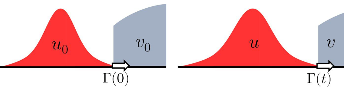
Finally, if reaction rates $c_{1}$ and $c_{2}$ are of Case 3, then we get immovable behavior of the limiting interface as follows.

Figure 3 explains a non-trivial example of interface evolution corresponding to Case 3. Also for this case, there might exist some jump points for $v_{0}$ at the interface so that we conduct the same procedure as in Case 2 to find $u^{N}_{0}$ and $v^{N}_{0}$ which fulfill the requirements (A1) and (B3).

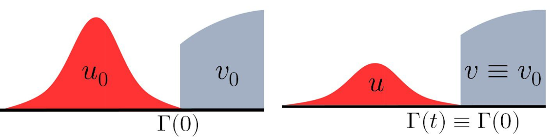
In Case 1, starting from initial densities separated in two particle-phases, though, the initial interface vanishes instantaneously and type-$1$ particles occupy the whole space (see Section 6). This is intuitively caused by weak killing effect of type-$2$ particles (recall that time evolution of type-$2$ particles is composed only of annihilation since they do not diffuse), which makes them die out in an instant. On the other hand, in Case 2 and Case 3, interfaces are created and they move according to the two-phase Stefan problem in Case 2 (see Section 7) while they does not move at all in Case 3 (see Section 8). In Case 2, roughly speaking, multiplication of some monomial of the density of type-$2$ particles to the second equation of (3.1) enables us to obtain another reaction-diffusion system whose reaction terms coincide up to a positive constant (but we have to replace a locally scattered product into a spatially-homogeneous one by using uniform boundedness of spatial derivatives). Therefore, this case is essentially considered in [4] but the diffusion coefficient for type-$2$ particles is zero in our model and consequently we get a one-phase free boundary problem instead. Finally, in Case 3, type-$1$ particles have weak killing effect. Comparing to Case 1, it seems that type-$1$ particles die out. However, since type-$2$ particles has no ability to diffuse, they do not invade the territory of type-$1$ particles so that the initial interface does not move at all.

As we noted at the beginning of this paper, the proof of our main theorems is based on Yau’s relative entropy method which is introduced in [12] combined with a (deterministic) result which ensures a solution of a semi-discretized system converges to a solution of a continuous PDE system . In this section, we explain what we need to prove the main theorems in detail. To see that, we first introduce a discretized version of macroscopic equations which characterize time evolution of density. For every fixed $T>0$, let $u^{N}=u^{N}(t,x)$ and $v^{N}=v^{N}(t,x)$ be a unique solution of the following semi-discretized reaction-diffusion system

for every $t\in[0,T]$ and $x\in\mathbb{T}^{d}_{N}$. Here $\Delta^{N}$ denotes the discrete Laplacian defined by

for every $u=\{u(x)\}_{x\in\mathbb{T}^{d}_{N}}$ and $c_{i,x}$ is defined by $c_{i,x}(u(t),v(t))=c_{i}(\tau_{x}u(t),\tau_{x}v(t))$ for each $i=1,2$ and every $[0,1]$-valued functions $u=\{u(x)\}_{x\in\mathbb{T}^{d}_{N}}$ and $v=\{v(x)\}_{x\in\mathbb{T}^{d}_{N}}$, and non-negative functionals $c_{1}$ and $c_{2}$ on $[0,1]^{\mathbb{T}^{d}_{N}}\times[0,1]^{\mathbb{T}^{d}_{N}}$ defined in Section 2. The semi-discretized system (3.1) is a system of ODEs whose solutions are contained in the interval $(0,1)$ uniformly in $(t,x)\in[0,T]\times\mathbb{T}^{d}_{N}$ for every $N\in\mathbb{N}$ and thus it has a unique pair of time-global solution. Indeed, in Lemma 5.3 we prove $0<u^{N}(t,x),v^{N}(t,x)<1$ for every $t\in[0,T]$ and $x\in\mathbb{T}^{d}_{N}$ provided $0<u^{N}(0,x),v^{N}(0,x)<1$ for all $x\in\mathbb{T}^{d}_{N}$.

In Section 5, we give some general estimates derived for the solution of this semi-discretized system (3.1). Moreover, let $\{u^{N}(t,\theta)\}_{t\in[0,T],\theta\in\mathbb{T}^{d}}$ and $\{v^{N}(t,\theta)\}_{t\in[0,T],\theta\in\mathbb{T}^{d}}$ be macroscopic functions on $Q_{T}:=[0,T]\times\mathbb{T}^{d}$ defined by

References

- [1] H. Brézis: Analyse Fonctionelle, Masson, Paris, 1983.
- [2] E. C. M. Crooks, E. N. Dancer, D. Hilhorst, M. Mimura and H. Ninomiya: Spatial segregation limit of a competition-diffusion system with Dirichlet boundary conditions, Nonlinear Anal. Real World Appl., 5 (2004), 645-665.
- [3] E. N. Dancer, D. Hilhorst, M. Mimura and L. A. Peletier: Spatial segregation limit of a competition-diffusion system, European J. Appl. Math., 10 (1999), 97-115.
- [4] A. De Masi, T. Funaki, E. Presutti and M. E. Vares: Fast-reaction limit for Glauber-Kawasaki dynamics with two components, ALEA, Lat. Am. J. Probab. Math. Stat., 16 (2019), 957-976.
- [5] T. Funaki: Free boundary problem from stochastic lattice gas model, Ann. Inst. H. Poincaré, Probab. Statist., 35 (1999), 573-603.
- [6] T. Funaki and K. Tsunoda: Motion by mean curvature from Glauber-Kawasaki dynamics, J. Stat. Phys., 177 (2019) 183-208.
- [7] D. Hilhorst, R. van der Hout and L. A. Peletier: The fast reaction limit for a reaction-diffusion system, J. Math. Anal. Appl., 199 (1996), 349-373.
- [8] D. Hilhorst, R. van der Hout and L. A. Peletier: Nonlinear diffusion in the presence of fast reaction, Nonlinear Annal., 41 (2000), 803-823.
- [9] M. Iida, H. Monobe, H. Murakawa and H. Ninomiya: Vanishing, moving and immovable interfaces in fast reaction limits, J. Differential Equations, 263 (2017), 2715-2735.
- [10] M. Jara and C. Landim: Nonequilibrium central limit theorem for a tagged particle in symmetric simple exclusion, Ann. Inst. H. Poincaré Probab. Statist., 42 (2006), 567-577.
- [11] M. Jara and O. Menezes: Non-equilibrium fluctuations for interacting particle systems, arXiv:1810.09526.
- [12] H.-T. Yau: Relative entropy and hydrodynamics of Gunzburg-Landau models, Lett. Math. Phys., 22 (1991), 63-80.