Current-induced atomic motion, structural instabilities, and negative temperatures on molecule-electrode interfaces in electronic junctions
Abstract
Molecule-electrode interfaces in molecular electronic junctions are prone to chemical reactions, structural changes, and localized heating effects caused by electric current. These can be exploited for device functionality or may be degrading processes that limit performance and device lifetime. We develop a nonequilibrium Green’s function based transport theory in which the central region atoms and, more importantly, atoms on molecule-electrode interfaces are allowed to move. The separation of time-scales of slow nuclear motion and fast electronic dynamics enables the algebraic solution of the Kadanoff-Baym equations in the Wigner space. As a result, analytical expressions for dynamical corrections to the adiabatically computed Green’s functions are produced. These dynamical corrections depend not only on the instantaneous molecular geometry but also on the nuclear velocities. To make the theoretical approach fully self-consistent, the same time-separation approach is used to develop expressions for the adiabatic, dissipative, and stochastic components of current-induced forces in terms of adiabatic Green’s functions. Using these current induced forces, the equation of motion for the nuclear degrees of freedom is cast in the form of a Langevin equation. The theory is applied to model molecular electronic junctions. We observe that the interplay between the value of the spring constant for the molecule-electrode chemical bond and electronic coupling strength to the corresponding electrode is critical for the appearance of structural instabilities and, consequently, telegraphic switching in the electric current. The range of model parameters is identified to observe structurally stable molecular junctions as well as various different kinds of current-induced telegraphic switching. The interfacial structural instabilities are also quantified based on current noise calculations.
I Introduction
A molecular electronic junction is a single molecule chemically bonded to two macroscopic electrodes. The structural flexibility of the organic framework makes the current-induced atomic motion one of the most critical processes to the performance of molecular electronic devices. Atomic nuclei feel the tug of the tunneling electrons, which can induce nonequilibrium excitations in the molecular vibrations Ryndyk and Cuniberti 2007; Ryndyk et al. 2006; Galperin et al. 2007; Galperin et al. 2006a; Härtle et al. 2008, atomic rearrangements and rotations Tikhodeev and Ueba 2009; Roy et al. 2013, as well as large-scale current-driven conformational changes such as chemical reactions Lee and Ho 1999; Hla et al. 2000; Repp et al. 2006; Tikhodeev and Ueba 2009; Dzhioev and Kosov 2011; Dzhioev et al. 2013, bond rupturesStipe et al. 1997; Erpenbeck et al. 2018, telegraphic switching between multiple geometries Kim et al. 2010; Artes et al. 2014; Song et al. 2016; Cho et al. 2017; Kosov 2018; Xiang et al. 2014; Gurvitz et al. 2016; Rudge and Kosov 2019, and structural instabilities Weick et al. 2011; Pistolesi et al. 2008; Brüggemann et al. 2012; Micchi et al. 2015; Micchi et al. 2016; Avriller et al. 2018; Foti and Vázquez 2018; Weick et al. 2010. Current-induced forces exerted by out-of-equilibrium electrons on nuclei result in heating within the system, consequently straining molecular bonds and decreasing the functionality and lifespan of the system. The structural instabilities and switching between different conformations introduced by these interactions can be detrimental to the performance of a nanoscale system. From another perspective, the small size and high sensitivity of nanoscale junctions result in the capability of utilizing the current-induced forces as a mechanism for satisfying specific tasks: such as a molecular switch, mass and charge sensors, as well as nanoscale motors Eom et al. 2011. Moreover, the ability to directly manipulate temperature within the system using quantum mechanical effects such as quantum back-action enables new ways of quantum control of nanomechanical systems Stettenheim et al. 2010.
One observed consequence of the sensitivity of a molecular junction to the voltage bias is voltage-induced breakage due to quantum heating: molecular junctions can rarely sustain experimentally more than 1-2 V of applied voltage bias Schulze et al. 2008; Sabater et al. 2015. In molecular junctions, the energy of the flowing current is dispersed by inelastic scattering of electrons through the system. There is a delicate balance between the heating due to inelastic processes and heat dissipation within molecular systems; if a molecular junction is allowed to get too hot, instabilities and bond breakages can occur Foti and Vázquez 2018. The absence of the fluctuation-dissipation theorem, which balances these energy gain and loss processes in equilibrium, complicates considerably the theoretical consideration Bode et al. 2011; Bode et al. 2012; Dzhioev et al. 2013.
Another experimental manifestation of the current-induced forces in molecular junctions is the telegraph noise, which is the stochastic switching over time between two different values of the electric current. Numerous studies of molecular junctions have observed a discrete switching between two or more states in the system, which can be observed via analysis of the measured time-evolution of the current through the system Kim et al. 2010; Artes et al. 2014; Song et al. 2016; Cho et al. 2017; Xiang et al. 2014. While the exact source of telegraph noise in molecular junctions depends on the particular experimental configuration, it is usually due to either dynamic switching between two different conformations of the molecular bridge or, more often, due to bond fluctuations of the metal-molecule contact. The telegraph noise is heavily influenced by the presence of inelastic interactions between the tunneling electrons and nuclear degrees of freedom within the junction, which can provide the energy required for conformational changes. In order to ensure the stability of the current-voltage properties of a given molecular junction, we would generally like to avoid these fluctuations between states which may have unforeseen effects. However, perhaps the existence of telegraph noise for specific systems may enable them to replicate certain functions of electric circuits due to their inherent molecular properties Xiang et al. 2014.
Many theoretical approaches have been developed to deal with nuclear dynamics in molecular junctions, which generally fall into two categories. The first is based on treating nuclear motion as harmonic vibrations around equilibrium and typically assuming linearized electron-vibration coupling. Then either a master equation based method Mitra et al. 2004; Koch and von Oppen 2005; Härtle and Thoss 2011; May 2002; Schinabeck et al. 2016; Agarwalla et al. 2015; Kosov 2017a; Kosov 2017b; Dzhioev and Kosov 2014; Dzhioev and Kosov 2015 or a NEGF method Ryndyk et al. 2006; Dahnovsky 2007; Galperin et al. 2006b; Ryndyk et al. 2006; Ryndyk and Cuniberti 2007; Härtle et al. 2008; Wilner et al. 2014; Erpenbeck et al. 2015; Frederiksen et al. 2007 is used to describe the system. All theoretical methods in the first category assume that the amplitudes of nuclear motion are small and nuclei vibrate harmonically about the zero-current equilibrium geometry. Furthermore, they require that either electron-vibration coupling or molecule-electrode interaction should be small, allowing for a perturbative treatment.
The second approach has gained significant attention recently; it is based on the non-equilibrium Born-Oppenheimer approximation – nonequilibrium quantum electrons exert non-conservative stochastic forces on the nuclear degrees of freedom, which are treated classically Pistolesi et al. 2008; Weick et al. 2010; Lu et al. 2010; Dzhioev and Kosov 2011; Bode et al. 2011; Bode et al. 2012; Dzhioev et al. 2013; Galperin and Nitzan 2015; Dou and Subotnik 2017a; Dou et al. 2017; Dou and Subotnik 2018; Kershaw and Kosov 2017; Kershaw and Kosov 2018; Kershaw and Kosov 2019. It does not assume that the amplitude of nuclear motion is small or harmonic, nor is it required that the electron-vibration interaction be treated as small or linear in nuclear displacement. This approach casts the stochastic nuclear dynamics in the form of a Langevin equation. There are a number of varying methods for calculating the friction tensor and random force which are the main ingredients of the Langevin equation. These include the use of NEGF methods Plihal and Langreth 1998; Plihal and Langreth 1999; Bode et al. 2012; Thomas et al. 2012; Dou and Subotnik 2017a; Dou and Subotnik 2018; Dou and Subotnik 2017b, which we will also employ in this paper, as well as scattering theory approachesBode et al. 2012; Bode et al. 2011; Mozyrsky et al. 2006; Bennett et al. 2010, path integral methods and influence functional methodsBrandbyge et al. 1995; Daligault and Mozyrsky 2007; Lü et al. 2012.
With a handful of exceptions Dou and Subotnik 2017a; Dou and Subotnik 2018; Coffman and Subotnik 2018; Erpenbeck and Thoss 2019; Dou and Subotnik 2017b; Erpenbeck et al. 2018, all these theoretical approaches largely focus on nuclear motion localized in the central region; however, the motion at the molecule-electrode interface is at least equally important. Large amplitude conformational changes such as chemical reactions, switching between different geometries, localized heating, and electromigration of atoms predominantly occur on the interface in molecular electronic junctions. Our goal is to derive a Langevin equation to describe the dynamics of nuclear motion on molecule-electrode interfaces, and then utilize computational simulations to provide insight on the impacts of nuclear motion on the measured current noise through the system with relevance to physical applications. To this end, we do not only obtain the Langevin equation with all parameters fully determined from adiabatic Green’s functions, but also solve approximately the time-dependent Kadanoff-Baym equations along the generated stochastic trajectory. The solution of the Kadanoff-Baym equations makes use of Wigner space and gradient expansion methods to separate fast electronic and slow nuclear time-scales. As a result, we have produced a theory where the nuclear motion on molecule-electrode interfaces and electronic dynamics is treated self-consistently.
The paper is organized as follows. Section II describes the theory: solution to the Kadanoff-Baym equations, derivation of dynamical corrections to the current, and also derivation of all components of the current-induced forces in terms of NEGF. The physical model and the results of calculations are presented in section III. The conclusions of the paper are summarized in section IV. The technical details of electronic diffusion coefficient derivation is relegated to the appendix.
We use atomic units throughout the paper, both in derivations and in the calculations ().
II Theory
II.1 Hamiltonian
Let us consider the general tunneling Hamiltonian which describes a molecular junction
| (1) |
Here is the time-dependent Hamiltonian for the molecule, is the Hamiltonian for the left lead and is the Hamiltonian for the right lead. The terms and are time-dependent and describe the tunneling of electrons between the molecule and the left and right leads, respectively.
Suppose that describes the time-dependent trajectory of atomic coordinates including atoms on the molecule-lead interfaces. We assume that is a classical variable. To simplify the notation, we take as a scalar rather than a multidimensional vector throughout derivations in the paper, but all our results can be readily extended to the case of many classical variables.
We assume that the molecule contains non-interacting electrons and is described by some quadratic Hamiltonian
| (2) |
Here and are fermionic creation and annihilation operators for single-particle states localized in the molecular space; is the corresponding matrix elements of the molecular Hamiltonian. The left and right leads of the molecular junction are macroscopic reservoirs of non-interacting electrons
| (3) |
where creates an electron in the single-particle state of the (left/right) lead with energy , and is the corresponding electron annihilation operator. The tunneling interaction is
| (4) |
where the tunneling amplitudes depend on the molecular junction geometry.
The molecular Hamiltonian as well as the tunneling molecule-lead interactions and are explicitly time-dependent via the dependence on the time-evolution of the molecular junction geometry .
II.2 Non-Adiabatic expansion of Kadanoff-Baym equations in Wigner space
The basic building blocks in our derivation are non-adiabatic (exact) retarded, advanced and lesser molecular Green’s functions, calculated with a fully time-dependent Hamiltonian along a given trajectory :
| (5) |
| (6) |
and
| (7) |
These Green’s functions are computed using a system of coupled Kadanoff-Baym equations of motion (note that we consider the retarded and advanced equations collectively) Haug and Jauho 2010
| (8) |
and
| (9) |
The Green’s function, Hamiltonian , and self-energies are written in the Kadanoff-Baym equations as matrices in molecular space and the molecular orbital indices are omitted here and in the subsequent derivations for brevity. Here means .
To transform these equations into the Wigner space, we define the central time and relative time as
| (10) |
and
| (11) |
and introduce the Wigner transform of an arbitrary Green’s function component
| (12) |
The inverse Wigner transform from the Wigner space to the time domain takes the form
| (13) |
Applying the Wigner transform to both sides of (8) and (9) yields the Kadanoff-Baym equations of motion in the Wigner space
| (14) |
and
| (15) |
The equations of motion in the Wigner space are solved by treating the time derivatives with respect to the central time as a small parameter. This treatment means that we treat changes in the self-energies and Green’s functions as slow with respect to central time and fast with respect to relative time. Central time dependence arises through the classical variable and so the slow variation with respect to central time is associated with slow nuclear dynamics. The relative time is associated with the electronic time-scale and, in our case, the characteristic tunneling time for the electron to transport across the molecule. Therefore the small parameter in our theory will be the ratio between the characteristic time-scales of nuclear motion and electron tunneling. The tunneling timescale can be estimated as where is the molecular level broadening due to the molecule-lead coupling. The time-scale for nuclear dynamics is given by where is the characteristic frequency for nuclear motion. Therefore the small parameter in our theory is .
The solution described below follows closely the ideas of previous authorsBode et al. 2012; Dou and Subotnik 2017b; Dou and Subotnik 2018; Kershaw and Kosov 2017; Kershaw and Kosov 2018; Kershaw and Kosov 2019. The exponential operators in Eqs.(14,15) are expanded up to the first order in the time derivatives, where we result in a truncated equation of motion for the retarded, advanced and lesser components of the Green’s functions
| (16) |
and
| (17) |
Here the function notation of the self-energies and Green’s functions have been suppressed for brevity. We now solve each of the equations above separately: first considering the retarded/advanced equation of motion followed by the lesser equation. Finding solutions with the derivatives up to the first order requires perturbative expansions of both the Green’s functions and self-energies. In doing so, we expand all Green’s function and self-energy components into a power series in terms of the small parameter:
| (18) |
and
| (19) |
Here the terms and depend on the instantaneous nuclear geometry only, while and depend on the nuclear geometry and are linear in velocities .
Substituting (18) and (19) into (16) and splitting the equation based on order results in the equations
| (20) |
and
| (21) |
The equation for the zeroth order is easily solved to give
| (22) |
which is the standard, adiabatic retarded/advanced Green’s function . Considering now the first order equation of motion (21), we rearrange in terms of to obtain
| (23) |
Here we have defined the quantities and in the interest of brevity, a convention that will be used for the remainder of this derivation.
The first order Green’s function derivatives are found to be
| (24) |
and
| (25) |
This enables us to simplify (23) to
| (26) |
Notice that that the Green’s functions, self-energies, and their derivatives will become scalars for transport in the single molecular energy level case and therefore the commutator term will vanish.
We now consider the equation of motion for the lesser Green’s function which is given by (17). The expansions (18) and (19) are substituted into (17) and, as before, split based on order to give
| (27) |
and
| (28) |
The zeroth order equation is easily solved to give
| (29) |
which is again the standard expression for the adiabatically computed lesser Green’s function . Considering now the first order equation, we first compute explicit expressions for the lesser Green’s function derivatives:
| (30) |
and
| (31) |
By substituting these expressions into (28) and rearranging the equation in terms of , we find
| (32) |
It remains to calculate the expressions for our self-energies. Beginning with our general definition for the self-energy in real-time, we then apply the Wigner transform which allows us to extract an adiabatic case along with our first non-adiabatic correction. The exact self-energy computed in real time isHaug and Jauho 2010
| (33) |
where is the non-interacting Green’s functions for the separated leads. Application of the Wigner transform to (33) yields
| (34) |
where we have used and to denote the central-time derivative with respect to and respectively. Expansion of the above exponential enables us to partition the equation into orders of magnitude of such that we find our adiabatic self-energy and corrections as
| (35) |
and
| (36) |
Here we have introduced the self-energy-like quantities:
| (37) |
and
| (38) |
where and are their respective Wigner transformations. The derivative of the tunneling amplitude with respect to our classical coordinate is defined as
| (39) |
By enacting an equivalent derivation as for the self-energy, we can decompose these new quantities into an adiabatic term and a first-order correction as given by:
| (40) |
| (41) |
| (42) |
and
| (43) |
where
| (44) |
II.3 Dynamical Corrections to Time-Dependent Electric Current
In section II-B, we obtained first-order dynamical corrections to the retarded, advanced, and lesser central region Green’s functions. Let us now obtain an expression for the current that includes first order dynamical corrections due to the motion of interfacial atoms. We begin with the general expression for the electric current flowing into the molecule from the lead at time Haug and Jauho 2010:
| (45) |
To facilitate a transformation to the Wigner space, we introduce the two-time function
| (46) |
which becomes the electric current if
| (47) |
A transformation into the Wigner space yields
| (48) |
Following the ideas of the previous section, we now expand the exponential operators up to the first order, along with including our non-adiabatic corrections to the Green’s functions and self-energies. We then perform an inverse Wigner transform back to real time, in which we set . This yields the equation for our current in real time in terms of an adiabatic component and a first order correction. The adiabatic component is found to be
| (49) |
while the first order correction is given by
| (50) |
| (51) |
and
| (52) |
Our final general expressions for the current are then given by
| (53) |
and
| (54) |
II.4 Current-induced forces: adiabatic, viscous, and random component
We have obtained analytical solutions to the Kadanoff-Baym equations for Green’s functions as functions of instantaneous positions and velocities. Therefore, for any given trajectory we know how to compute all system observables. Our aim here is to derive a Langevin-like equation to obtain the stochastic trajectory for the molecular junction geometry . Our derivation follows the ideas introduced by von Oppen et al.Bode et al. 2012, then later expanded upon by Subotnik and Dou Dou and Subotnik 2017b; Dou and Subotnik 2018.
The derivation starts on a purely quantum-mechanical footing, by considering quantum position and momentum operators ( and ) which correspond to the classical variable . The Heisenberg equation of evolution for the momentum operator gives the expression for the quantum force
| (55) |
where is the full Hamiltonian of the system. Note that in contrast to previous sections, we have been careful to make explicit the operator notation so that the quantum and classical quantities are easily distinguishable. In the coordinate representation, ; therefore
| (56) |
which when making a substitution for (1) becomes
| (57) |
where we have added the classical potential to the Hamiltonian where . Making a substitution for each Hamiltonian results in
| (58) |
where the quantity is given by (39). First, we compute the average of the force operator at time and then we introduce the stochastic fluctuations around this average. The force exerted by electrons is
| (59) |
and its average can be conveniently expressed in terms of Green’s functions
| (60) |
We now introduce our auxiliary two-time function as
| (61) |
which has the property . As previously, we first utilize the Dyson equation for our Green’s functions spanning the molecular space and the leads . In doing so, we express in terms of molecular space quantities:
| (62) |
where our self-energy-like quantities (38) and (37) have appeared once again in the equation. Taking a trace over the molecular states and performing a transformation into the Wigner space yields
| (63) |
Now, by taking the inverse Wigner transform and letting such that , we decompose our classical force into an adiabatic component and a velocity-dependent correction (which will correspond to our viscosity force). The adiabatic component of the force is given by
| (64) |
while the velocity dependent first order component is given by
| (65) |
We note that the second term reduces to zero as
| (66) |
This can be further simplified through the use of (51) along with the following identity:
| (67) |
Our final expression for the velocity-dependent force is then given by
| (68) |
This expression is linear in velocity and results in the viscosity force in the Langevin equation for .
To complete the Langevin equation, we need to define the diffusion coefficient as a time correlation of the force variations
| (69) |
where
| (70) |
Through a tedious derivation, one can compute an explicit expression for the diffusion coefficient, a derivation that has been relegated to Appendix A. One can show that
| (71) |
III results
III.1 Model
The molecular bridge is modeled by a single molecular orbital with energy as
| (72) |
where is a classical time-dependent coordinate. In our case models a bond-length between the molecule and the left lead. This -dependence of the molecular orbital comes from the voltage drop across the junction
| (73) |
where
| (74) |
is the electric field across the junction and
| (75) |
is the -independent energy level shift. Here we use and to denote the positions of the left and right leads, while and are the left and right lead chemical potentials. The equilibrium bond-length is denoted by . The applied voltage bias will be applied symmetrically and in all our calculations.
We assume that the coupling to the right electrode is rigid and the coupling to the left depends on the bond-length:
where the function is taken in the form of the overlap between two 1s orbitals separated by distance as given by
| (79) |
and and are two constants. This choice of coordinate dependence mimics the behavior of a generic isotropic chemical bond.McQuarrie 2007
We assume that the coupling to the left lead is time-dependent and the time-dependence comes from the variations of the bond-length between the molecule and the left lead. The choice of the left electrode is completely arbitrary, we can chose the linkage to the right electrode to be time-dependent as well.
We will use the wide-band approximation for the leads and, in this limit, the leads self-energy components become
| (80) |
| (81) |
and
| (82) |
Here and we have introduced the standard level broadening function
| (83) |
where is the density of single-particle states in lead . Notice that the retarded/advanced self-energies for the left lead have lost their energy dependence on in the wide-band limit and retarded/advanced self-energies for the right lead become constants.
In the considered case of electron transport through a single resonant level, the expressions for the non-adiabatic corrections can be further simplified since the Green’s functions and self-energies are no longer matrices, in addition to the wide-band approximation killing some derivatives. The first order correction to the lesser Green’s function becomes
| (84) |
It is expressed in terms of standard adiabatic (instantaneously computed along the nuclear trajectory ) Green’s functions
| (85) |
The adiabatic electric current is
| (86) |
while the first order velocity-dependent non-adiabatic correction to the electric current is
| (87) |
The adiabatic force is
| (88) |
and the dissipative force is given by
| (89) |
Finally, the diffusion coefficient is
| (90) |
The time-evolution of the bond-length is given by the Langevin equation
| (91) |
Here, the adiabatic force is given by Eq.(88), the electronic viscosity is defined from velocity dependent contribution to the force (89) as
| (92) |
and is a white noise random force with diffusion coefficient (90). The classical potential is taken to be harmonic
| (93) |
where is the equilibrium bond-length and is the spring constant associated with the bond strength.
III.2 Calculations


Each of our calculations utilize a common set of unchanging parameters: the bandwidth for numerical integration is set to [-5, 5]; left and right lead temperatures are set to be equal (); the reduced mass associated with the chemical bond is ; the molecule is always strongly coupled to the left lead with and ; and the equilibrium bond-length is . All numerical values in the text and figures are given in atomic units.
III.2.1 Electronic friction, diffusion coefficient, and local effective temperature
We first study how the parameters of the model control the three main ingredients of the Langevin equation: the diffusion coefficient, viscosity, and adiabatic force. Fig. 1(a) shows the diffusion coefficient as a function of the bond-length. The amplitude of the random force is the square root of the diffusion coefficient. As seen in Fig.1(a), the diffusion coefficient has a strong dependence on the bond-length, reaching its maximum at the equilibrium bond-length and then decaying to zero as the bond stretches or contracts. As physically expected, the amplitude of the random force increases as the voltage becomes larger.
The viscosity is shown in Fig.1(b). At small voltages the viscosity behavior mirrors the diffusion coefficient’s dependence on the bond-length. This is not surprising if one recalls the fluctuation-dissipation theorem which relates the ratio of the diffusion coefficient and viscosity to the temperature, and temperature should not deviate significantly from the equilibrium value for small voltages. If the voltage is increased, we start to observe regions of negative viscosity which energize the stretching/contraction of the bond rather than dampening its oscillations as one may expect from the viscous force. This negative viscosity phenomenon has been previously observed for similar theoretical systems using varying modeling techniquesBode et al. 2012; Lü et al. 2011; Metelmann and Brandes 2011.
Fig. 1(c) shows viscosity as a function of bond-length computed at of applied voltage. Once the level moves away from the resonance position , the second peak in the viscosity starts to shift closer to the equilibrium bond-length. The second peak occurs when the energy of the level intersects the Fermi level of the right lead, such that electrons are easily able to transition between the lead and the resonance level, while the left lead is essentially disconnected due to the exponential coupling decay.


In analogy to the fluctuation-dissipation theorem Zwanzig 2001, it is instructive to define an effective temperature as
| (94) |
This effective temperature is an intuitively clear physical quantity which reveals information on the steady-state spatial distribution of kinetic energy within the junction and is related to current-induced localized heating or cooling effects.


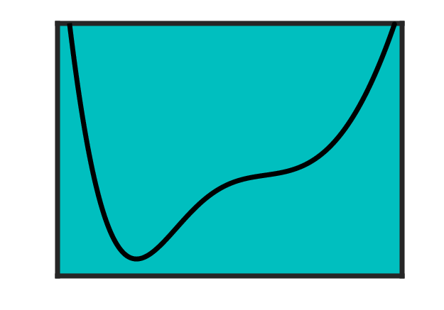
It is clear from Fig.2(a) that in the equilibrium case (zero applied voltage), the fluctuation-dissipation theorem is satisfied as is independent of and equals to K, exactly the temperature of left and right leads. Once the voltage is increased, the current carrying electrons produce significant local heating in the junction leading to the rise of the effective temperature. The coordinate dependence of effective temperature has a small dip at equilibrium bond-length and then reaches its maximum value if the bond is stretched.
In Fig.2(d), we observe a region of parameters in our junction in which the effective temperature becomes negative, such that the nucleus has no defined steady-state local kinetic energy in this region and as such, the kinetic energy of the nuclei will continue to increase if constrained to this region.
Next, we compute the adiabatic potential as a function of bond-length. By combining the classical potential and integrating our adiabatic force computed by Eq.88, we obtain the adiabatic potential Dzhioev and Kosov 2011
| (95) |
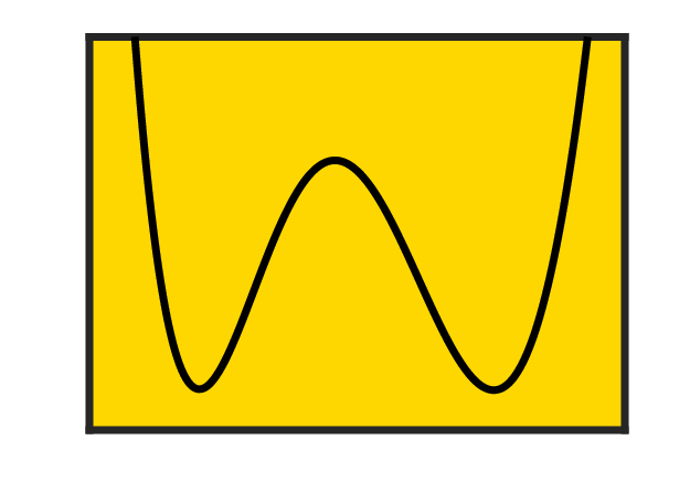
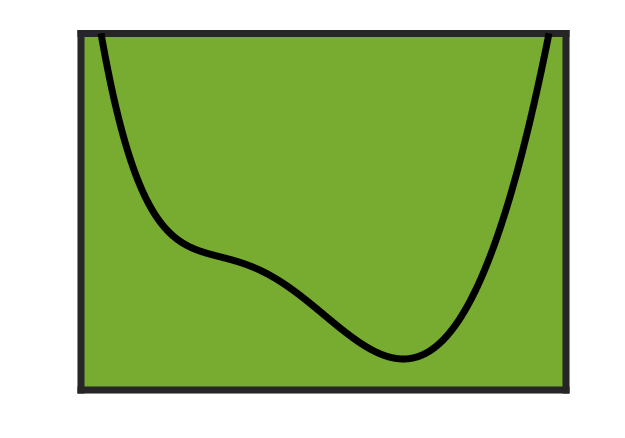
Notice that the lower limit in this integral is completely arbitrary and serves as a reference point for the computed potential energy. We use in all our calculations. We observe in 3(a) and 3(b) the possibility of different potential regimes in which we may observe two separate stable minima.
These regimes are summarized according to the changing bond spring constant and coupling in Figure 4. There is a narrow region of bistability. Once we move away from this region, one minimum starts to dominate until the other minimum disappears completely. As one increases the voltage, the bistable yellow region becomes wider and shifts towards smaller values of the spring constant.




III.2.2 Current
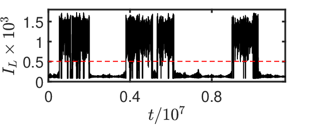
In this section, we show results for the current computed along a given trajectory of the bond-length time-evolution obtained from the solution of the Langevin equation. To compute a trajectory , we utilize an m-BAOAB algorithm provided by Sachs et alSachs et al. 2017, which enables a numerical solution of the Langevin equation with a coordinate dependent viscosity and diffusion coefficient. The trajectory is used to compute Green’s functions, and current with first order dynamical corrections using the equation presented in section III.1. We consider three representative scenarios with very distinct nuclear dynamics: rigid chemical bonding (), intermediate chemical bonding (), and soft chemical bonding (). In the case of a rigid chemical bond, the bond-length oscillates around a single minima; this is reflected in the time dependence of current shown in Fig.5(a), 5(b). Both the electric current with dynamical corrections and the first order correction itself oscillate around single average values. Once the chemical bond becomes softer (), the length of the chemical bond switches between two states, spending roughly equal time in each. This behavior of the bond-length results into telegraphic switching of the current between two values as shown in Fig.5(c), 5(d). The first order dynamical correction is more noticeable in the more conducting state. For a soft molecule-lead chemical bond, , the bond-length experiences switching but has a preference for a specific value, as does the current.
III.3 Current noise
The temporal correlations between stochastic fluctuations of the electric current (current noise) have become a very important experimental and theoretical tool in studying transport properties of molecular junctions. Noise spectroscopy enables the study of the special features of a single-molecule junction, which are not accessible by standard current-voltage measurements. The experimental noise measurements provide significantly new information on fundamental mechanisms of electron transport in molecular junctions, such as atomistic details of the local environment and metal-molecule interfacesKim et al. 2010; Adak et al. 2015, coupling between electronic and vibrational degrees of freedomGalperin et al. 2006a; Secker et al. 2011; Kumar et al. 2012; Schinabeck et al. 2014, identifications of the individual conduction transport channelDjukic and van Ruitenbeek 2006; Wheeler et al. 2010; Tsutsui et al. 2010; Cho et al. 2017, and mechanical stability of the junctionXiang et al. 2014.


Current noise is formally defined as
| (96) |
where describes the instantaneous deviation of the electric current at time from its average value and is the anti-commutator. Eq.(96) involves two averages: is the quantum expectation value over electronic degrees of freedom and is the time average over the classical motion of the nuclei. The time average is equivalent to the ensemble average over many realizations of geometries of the molecular junction. The current noise power spectrum is the Fourier transformation of (96)
| (97) |
The electric current noise provides valuable information about the system and originates from multiple factors: (a) the quantum nature of electrons, discreteness of charge, Pauli exclusion principle, shot noise, and the finite temperature of electrons; (b) various types of quantum correlations between current-carrying electrons, which are not present in our model; (c) and finally, the ”mechanical” noise due to current-induced changes to the molecular junction geometry. Generally the total noise is not simply the addition of (a), (b), and (c) contributions; there is a cross interference between different contributions. However, within our approach the distinctly different time-scales of fast electronic and slow nuclear motion enables the separation of the mechanical noise contributionWeick et al. 2011. The characteristic time scale of shot noise decay is , whereas the noise due to nuclear motion appears on much longer times. Hence the noise induced by geometrical fluctuations dominates the noise power spectrum at low frequencies, and can exceed the shot noise contribution by orders of magnitude Weick et al. 2011.
In what follows we focus on the ”mechanical” noise as
| (98) |
where the current fluctuation at time is
| (99) |
The Fano factor is
| (100) |
The variance and mean of a Poisson process is equal, therefore the Fano factor can be used to characterize electron transport as either a sub-Poissonian (), Poissonian (), or super-Poissonian () process. Indeed, super-Poissonian or sub-Poissonian noise is caused by a host of very interesting and often hidden physical effects.

Figs.6(a) and 6(b) show Fano factors computed as a functions of the applied voltage and spring constant . The presence of telegraphic switching between two minima in a bi-stable adiabatic potential results in the gigantic enhancement of the Fano factor, indicating that the electron transport is a super-Poissonian process. The behavior of the Fano factor depends on a number of factors relating to the microscopic details of the Langevin dynamics in a locally heated adiabatic potential.
This behavior of the Fano factor can be rationalized based on the following observations. The only negative contributions to the integral over time in the current noise (98) are on the boundaries when the current crosses the mean. For the bi-stable case, this generally occurs only when the current switches between stable states. It is an intuitive notion to then conclude that larger switch rates will have an effect on decreasing the Fano factor (however having no switches at all will minimize it).
The size of the positive contribution to the current noise is dependent on two factors: firstly, the size of the fluctuations around the mean which correspond to the difference in current values between two configurations; and secondly, the ratio of time spent in each minimum. An increase to the applied voltage results in a larger fluctuation around the mean and as such, one would expect this to have an effect on increasing the Fano factor. However, this effect is counteracted by an increase to the mean current, which stays in the denominator of the Fano factor (100). Additionally, the noise should be maximized when the mean current is directly in between our two current states; this occurs when the nucleus spends approximately equal time in each minimum. Therefore, the two key parameters to control the Fano factor are the average switch rate (a single switch being a transition from one minimum to the other) shown in Fig.6(c), as well as the average waiting time (the average amount of time spent waiting in a minima before switching out) shown in Fig.6(d). To maximize the Fano factor, one wants to keep the switch rate between conformations as small as possible but at the same the waiting times in both conformations should be comparable. For example, let us consider the case of . As the voltage increases, the difference in effective temperatures between the left and right minima increases as well, such that the left is substantially hotter, which will decrease the time spent waiting in the left minimum. In addition, the large applied voltage will physically deform the adiabatic potential in a manner akin to Fig.3(b), decreasing the depth of the left minimum relative to the right. These factors each act to decrease the left minimum waiting time relative to the right (see Fig.6(d)). To compensate for this, the Fano factor peaks shifts towards smaller values of , which act to deepen the left minimum, thus having the opposing effect of increasing the left minimum waiting time.
In Fig.7, we observe the Fano factor as the adiabatic potential transitions over the three possible regimes in our system as the spring constant is altered. The Fano factor demonstrates a strong dependency on instabilities within the system, undergoing a large peak as the bi-stable regime is entered, before decreasing back to sub-Poissonian values in the mono-stable regimes. The peak is shifted towards lower values for the reasons outlined regarding Fig6(c). The peak decreases slowly into the blue mono-stable regime because the stable minimum is very close to the left lead, which yields a small mean current in this region. As such our Fano factor according to (100) is still large despite the adiabatic potential only being mono-stable.
IV conclusions
In this paper, we studied current-induced atomic motion on molecule-electrode interfaces in molecular electronic junctions. Structural changes on the interfaces are described in terms of a Langevin equation, which is obtained from the quantum mechanical first principles in which we extract the slow nuclear dynamics from Wigner space Green’s functions. The calculations of Green’s functions and consequently all molecular junction observables include dynamical velocity-dependent corrections to include non-adiabatic effects of nuclear motion into the calculation of electronic properties. We illustrate the theory by computing the transport properties of a model molecular junction: a single position-dependent resonant energy level which is coupled to the leads via a flexible (changing in time due to current flow) bond-length. The Langevin equation for the bond-length is integrated numerically and then the Green’s functions, electric current, and current noise are computed along the stochastic trajectory. We observe that even if the initial classical potential is harmonic, the effective adiabatic potential may develop bi-stability depending upon the parameters of the model. We mapped the shapes of the adiabatic potential in the parameter space of the model. The different regimes for bistability depend critically on the interplay between the softness of the linking electrode-molecule bond and the coupling to the corresponding electrode.
We introduce the concept of an effective local temperature using fluctuation-dissipation theorem ideas, which provides a useful insight on localized current-induced heating in molecular electronic junctions. We observe a region of parameters in our junction where the effective temperature becomes negative, which means the kinetic energy of nuclei will continue to increase if constrained to this region. The structural instabilities and localized heating on molecule-electrode interfaces are quantified in terms of the current noise and Fano Factor. These demonstrated the influence of the calculated effective temperatures and adiabatic potentials on the nuclear dynamics, in which super-Poissonian Fano factors on the order of were observed.
Appendix A Electronic diffusion coefficient
Computing the random white noise for our system starts by computing the quantity . Noting that allows us then to generate the expression
| (101) |
and so computing an expression for is reduced to calculating the quantities and .
The first term in (101) term can be computed by making an explicit substitution for in (58). This yields averages over strings of creation and annihilation operators which can be decomposed according to Wick’s theorem. An example of which is given by
| (102) |
where we have retained only the non-zero terms. It can be shown that the first term in these decompositions (involving no permutation of the creation/annihilation operators) will cancel exactly with the terms given in (which can be easily calculated using (57)). As a result, our random noise variance is then given by
| (103) |
where we have introduced our Green’s functions. Here we use indices without a bar () to represent an operator acting at time , while indices with a bar () act at time . At this point, we must decompose our Green’s functions into Green’s functions in the system space and Green’s functions in the leads. This involves applying our Dyson expansion to the Green’s functions spanning the leads and system space (eg. ), as well as decomposing the terms. For the purposes of this derivation, we will consider only a single term from (103) as the derivation can be applied similarly to the other terms in the equation. Consider
| (104) |
Applying our Dyson expansion to both Green’s functions and taking advantage of the commutativity of matrix elements will yield
| (105) |
By expanding this product and introducing our self-energy like quantities, we find
| (106) |
Applying a similar process for all terms in (103) yields the following expression:
| (107) |
where we have simplified the sum over central states into a trace and neglected time indices for brevity.
This equation must now be transformed into the Wigner space such that we can retrieve our diffusion coefficient. Beginning with
| (108) |
We integrate both sides with respect to which enables us to isolate as per
| (109) |
In taking the Wigner transform, we once again consider a single example term which we will denote .
where we have simply grouped terms together such that
| (110) |
and so on. Next, we transform it to the Wigner space using the Wigner convolution theorem and take the adiabatic limit, such that we obtain
| (111) |
All that then remains is to calculate the Wigner transform of our grouped variables and which is a relatively simple process. Applying this process to each term in 107, we find
| (112) |
We observe that some terms are conjugates of each other, while certain strings of functions appear frequently in different terms. With significant simplification, we find our final expression for the diffusion coefficient as
| (113) |
References
- Ryndyk and Cuniberti (2007) D. A. Ryndyk and G. Cuniberti, Phys. Rev. B 76, 155430 (2007).
- Ryndyk et al. (2006) D. A. Ryndyk, M. Hartung, and G. Cuniberti, Phys. Rev. B 73, 045420 (2006).
- Galperin et al. (2007) M. Galperin, M. A. Ratner, and A. Nitzan, J. Phys.: Cond. Matt. 19, 103201 (2007).
- Galperin et al. (2006a) M. Galperin, A. Nitzan, and M. A. Ratner, Phys. Rev. B 74, 075326 (2006a).
- Härtle et al. (2008) R. Härtle, C. Benesch, and M. Thoss, Phys. Rev. B 77, 205314 (2008).
- Tikhodeev and Ueba (2009) S. G. Tikhodeev and H. Ueba, Phys. Rev. Lett. 102, 246101 (2009).
- Roy et al. (2013) S. Roy, V. Mujica, and M. A. Ratner, The Journal of Chemical Physics 139, 074702 (2013) .
- Lee and Ho (1999) H. J. Lee and W. Ho, Science 286, 1719 (1999).
- Hla et al. (2000) S.-W. Hla, L. Bartels, G. Meyer, and K.-H. Rieder, Phys. Rev. Lett. 85, 2777 (2000).
- Repp et al. (2006) J. Repp, G. Meyer, S. Paavilainen, F. E. Olsson, and M. Persson, Science 312, 1196 (2006).
- Dzhioev and Kosov (2011) A. A. Dzhioev and D. S. Kosov, J. Chem. Phys. 135, 074701 (2011).
- Dzhioev et al. (2013) A. A. Dzhioev, D. S. Kosov, and F. von Oppen, J. Chem. Phys. 138, 134103 (2013).
- Stipe et al. (1997) B. C. Stipe, M. A. Rezaei, W. Ho, S. Gao, M. Persson, and B. I. Lundqvist, Phys. Rev. Lett. 78, 4410 (1997).
- Erpenbeck et al. (2018) A. Erpenbeck, C. Schinabeck, U. Peskin, and M. Thoss, Phys. Rev. B 97, 235452 (2018).
- Kim et al. (2010) Y. Kim, H. Song, D. Kim, T. Lee, and H. Jeong, ACS Nano, ACS Nano 4, 4426 (2010).
- Artes et al. (2014) J. M. Artes, M. Lopez-Martinez, I. Diez-Perez, F. Sanz, and P. Gorostiza, Small 10, 2537 (2014) .
- Song et al. (2016) Y. Song, H. Jeong, S. Chung, G. H. Ahn, T.-Y. Kim, J. Jang, D. Yoo, H. Jeong, A. Javey, and T. Lee, Scientific Reports 6, 33967 (2016).
- Cho et al. (2017) D. Cho, H. Lee, S. Shekhar, M. Yang, J. Y. Park, and S. Hong, Scientific Reports 7, 43411 (2017).
- Kosov (2018) D. S. Kosov, J. Chem. Phys. 148, 184108 (2018), .
- Xiang et al. (2014) D. Xiang, T. Lee, Y. Kim, T. Mei, and Q. Wang, Nanoscale 6, 13396 (2014).
- Gurvitz et al. (2016) S. Gurvitz, A. Aharony, and O. Entin-Wohlman, Phys. Rev. B 94, 075437 (2016).
- Rudge and Kosov (2019) S. L. Rudge and D. S. Kosov, Phys. Rev. B 100, 235430 (2019).
- Weick et al. (2011) G. Weick, F. von Oppen, and F. Pistolesi, Phys. Rev. B 83, 035420 (2011).
- Pistolesi et al. (2008) F. Pistolesi, Y. M. Blanter, and I. Martin, Phys. Rev. B 78, 085127 (2008).
- Brüggemann et al. (2012) J. Brüggemann, G. Weick, F. Pistolesi, and F. von Oppen, Phys. Rev. B 85, 125441 (2012).
- Micchi et al. (2015) G. Micchi, R. Avriller, and F. Pistolesi, Phys. Rev. Lett. 115, 206802 (2015).
- Micchi et al. (2016) G. Micchi, R. Avriller, and F. Pistolesi, Phys. Rev. B 94, 125417 (2016).
- Avriller et al. (2018) R. Avriller, B. Murr, and F. Pistolesi, Phys. Rev. B 97, 155414 (2018).
- Foti and Vázquez (2018) G. Foti and H. Vázquez, The Journal of Physical Chemistry Letters 9, 2791 (2018) .
- Weick et al. (2010) G. Weick, F. Pistolesi, E. Mariani, and F. von Oppen, Phys. Rev. B 81, 121409 (2010).
- Eom et al. (2011) K. Eom, H. S. Park, D. S. Yoon, and T. Kwon, Physics Reports 503, 115 (2011).
- Stettenheim et al. (2010) J. Stettenheim, M. Thalakulam, F. Pan, et al., Nature 466, 86 (2010).
- Schulze et al. (2008) G. Schulze, K. J. Franke, A. Gagliardi, G. Romano, C. S. Lin, A. L. Rosa, T. A. Niehaus, T. Frauenheim, A. Di Carlo, A. Pecchia, and J. I. Pascual, Phys. Rev. Lett. 100, 136801 (2008).
- Sabater et al. (2015) C. Sabater, C. Untiedt, and J. M. van Ruitenbeek, Beilstein J. Nanotechnol. 6, 2338 (2015).
- Bode et al. (2011) N. Bode, S. V. Kusminskiy, R. Egger, and F. von Oppen, Phys. Rev. Lett. 107, 036804 (2011).
- Bode et al. (2012) N. Bode, S. V. Kusminskiy, R. Egger, and F. von Oppen, Beilstein J. Nanotechnol 3, 144 (2012).
- Mitra et al. (2004) A. Mitra, I. Aleiner, and A. J. Millis, Phys. Rev. B 69, 245302 (2004).
- Koch and von Oppen (2005) J. Koch and F. von Oppen, Phys. Rev. Lett. 94, 206804 (2005).
- Härtle and Thoss (2011) R. Härtle and M. Thoss, Phys. Rev. B 83, 115414 (2011).
- May (2002) V. May, Phys. Rev. B 66, 245411 (2002).
- Schinabeck et al. (2016) C. Schinabeck, A. Erpenbeck, R. Härtle, and M. Thoss, Phys. Rev. B 94, 201407 (2016).
- Agarwalla et al. (2015) B. K. Agarwalla, J.-H. Jiang, and D. Segal, Phys. Rev. B 92, 245418 (2015).
- Kosov (2017a) D. S. Kosov, J. Chem. Phys. 146, 074102 (2017a) .
- Kosov (2017b) D. S. Kosov, J. Chem. Phys. 147, 104109 (2017b).
- Dzhioev and Kosov (2014) A. A. Dzhioev and D. S. Kosov, J. Phys. A: Math and Theor 47, 095002 (2014).
- Dzhioev and Kosov (2015) A. A. Dzhioev and D. S. Kosov, J. Phys. A: Math and Theor 48, 015004 (2015).
- Dahnovsky (2007) Y. Dahnovsky, J. Chem. Phys. 127, 014104 (2007).
- Galperin et al. (2006b) M. Galperin, A. Nitzan, and M. A. Ratner, Phys. Rev. B 73, 045314 (2006b).
- Wilner et al. (2014) E. Y. Wilner, H. Wang, M. Thoss, and E. Rabani, Phys. Rev. B 89, 205129 (2014).
- Erpenbeck et al. (2015) A. Erpenbeck, R. Härtle, and M. Thoss, Phys. Rev. B 91, 195418 (2015).
- Frederiksen et al. (2007) T. Frederiksen, M. Paulsson, M. Brandbyge, and A.-P. Jauho, Phys. Rev. B 75, 205413 (2007).
- Lu et al. (2010) J.-T. Lu, M. Brandbyge, and P. Hedegard, Nano Letters 10, 1657 (2010).
- Galperin and Nitzan (2015) M. Galperin and A. Nitzan, The Journal of Physical Chemistry Letters 6, 4898 (2015).
- Dou and Subotnik (2017a) W. Dou and J. E. Subotnik, Phys. Rev. B 96, 104305 (2017a).
- Dou et al. (2017) W. Dou, G. Miao, and J. E. Subotnik, Phys. Rev. Lett. 119, 046001 (2017).
- Dou and Subotnik (2018) W. Dou and J. E. Subotnik, Phys. Rev. B 97, 64303 (2018).
- Kershaw and Kosov (2017) V. F. Kershaw and D. S. Kosov, Journal of Chemical Physics 147, 224109 (2017).
- Kershaw and Kosov (2018) V. F. Kershaw and D. S. Kosov, The Journal of Chemical Physics 149, 044121 (2018).
- Kershaw and Kosov (2019) V. F. Kershaw and D. S. Kosov, Journal of Chemical Physics 150, 074101 (2019), 1809.07140 .
- Plihal and Langreth (1998) M. Plihal and D. C. Langreth, Phys. Rev. B 58, 2191 (1998).
- Plihal and Langreth (1999) M. Plihal and D. Langreth, Phys. Rev. B 60, 5969 (1999).
- Thomas et al. (2012) M. Thomas, T. Karzig, S. V. Kusminskiy, G. Zaránd, and F. von Oppen, Phys. Rev. B 86, 195419 (2012).
- Dou and Subotnik (2017b) W. Dou and J. E. Subotnik, Journal of Chemical Physics 146, 092304 (2017b).
- Mozyrsky et al. (2006) D. Mozyrsky, M. B. Hastings, and I. Martin, Phys. Rev. B 73, 035104 (2006).
- Bennett et al. (2010) S. D. Bennett, J. Maassen, and A. A. Clerk, Physical Review Letters 105, 217206 (2010).
- Brandbyge et al. (1995) M. Brandbyge, P. Hedegård, T. F. Heinz, J. A. Misewich, and D. M. Newns, Physical Review B 52, 6042 (1995).
- Daligault and Mozyrsky (2007) J. Daligault and D. Mozyrsky, Phys. Rev. E 75, 026402 (2007).
- Lü et al. (2012) J.-T. Lü, M. Brandbyge, P. Hedegård, T. N. Todorov, and D. Dundas, Phys. Rev. B 85, 245444 (2012).
- Coffman and Subotnik (2018) A. J. Coffman and J. E. Subotnik, Physical Chemistry Chemical Physics 20, 9847 (2018).
- Erpenbeck and Thoss (2019) A. Erpenbeck and M. Thoss, Journal of Chemical Physics 151, 191101 (2019).
- Haug and Jauho (2010) H. Haug and A. Jauho, Quantum Kinetics in Transport and Optics of Semiconductors (Springer, Berlin/Heidelberg, 2010).
- McQuarrie (2007) D. A. McQuarrie, Quantum Chemistry (University Science Books, Sausalito, California, 2007).
- Lü et al. (2011) J.-T. Lü, P. Hedegård, and M. Brandbyge, Physical Review Letters 107, 046801 (2011).
- Metelmann and Brandes (2011) A. Metelmann and T. Brandes, Physical Review B 84, 155455 (2011).
- Zwanzig (2001) R. Zwanzig, Nonequilibrium statistical mechanics (Oxford University Press, Oxford, 2001).
- Sachs et al. (2017) M. Sachs, B. Leimkuhler, and V. Danos, Entropy 19, 647 (2017).
- Adak et al. (2015) O. Adak, E. Rosenthal, J. Meisner, E. F. Andrade, A. N. Pasupathy, C. Nuckolls, M. S. Hybertsen, and L. Venkataraman, Nano Letters 15, 4143 (2015) .
- Secker et al. (2011) D. Secker, S. Wagner, S. Ballmann, R. Härtle, M. Thoss, and H. B. Weber, Phys. Rev. Lett. 106, 136807 (2011).
- Kumar et al. (2012) M. Kumar, R. Avriller, A. L. Yeyati, and J. M. van Ruitenbeek, Phys. Rev. Lett. 108, 146602 (2012).
- Schinabeck et al. (2014) C. Schinabeck, R. Härtle, H. B. Weber, and M. Thoss, Phys. Rev. B 90, 075409 (2014).
- Djukic and van Ruitenbeek (2006) D. Djukic and J. M. van Ruitenbeek, Nano Letters 6, 789 (2006) .
- Wheeler et al. (2010) P. J. Wheeler, J. N. Russom, K. Evans, N. S. King, and D. Natelson, Nano Letters 10, 1287 (2010) .
- Tsutsui et al. (2010) M. Tsutsui, M. Taniguchi, and T. Kawai, Nat. Commun. 1, 138 (2010).