Optimization methods can have implicit biases towards certain solutions Strand 1974; Morgan & Bourlard 1990; Neyshabur et al. 2014. In the context of deep network training, such biases have been shown to play key roles in shaping the properties of the learned model. For example, in binary classification of linearly separable data, among all linear separators that achieve the global minimum of the training loss, gradient descent (GD) converges to the maximum margin separator. This is true for shallow networks Soudry et al. 2018, as well as for deep linear fully-connected models Gunasekar et al. 2018b and deep nonlinear networks with homogeneous activation functions Lyu & Li 2020. Implicit biases have been studied in many different context, including for linear convolutional networks Gunasekar et al. 2018b, matrix factorization Gunasekar et al. 2017, weight normalization Wu et al. 2019, and with different loss functions Gunasekar et al. 2018a.

Perhaps the simplest mechanism through which GD and stochastic GD (SGD) can screen out solutions, is their inability to stably converge to sharp minima Jastrzębski et al. 2017; Wu et al. 2018; Simsekli et al. 2019. In fact, in some cases, GD can only converge to the flattest of all minima (see Section 2). However, interestingly, the effect that this has on the resulting trained model, is not yet fully understood. Keskar et al. 2016 suggested that flat minima tend to generalize better. This was somewhat supported by follow up works, showing that in SGD, larger step sizes and smaller batch sizes impose convergence to flatter minima, which indeed generalize better empirically Jastrzębski et al. 2017; Hoffer et al. 2017; Masters & Luschi 2018; Smith & Le 2017. However, Dinh et al. 2017 showed that for networks with ReLU activations, a re-parametrization of the weights can make any minimum arbitrarily sharper (without affecting generalization). This suggests that minimum sharpness is not directly related to generalization, thus begging the question: What does the sharpness of the minimum affect?

Our goal in this paper is to unveil the properties of flat minima in deep neural networks. We specifically focus on linear models trained with a quadratic loss and define the sharpness of a minimum to be its maximal Hessian eigenvalue, which is the factor affecting stable convergence of GD and SGD. We start by showing that all minima become sharper as the network gets deeper. We discuss and illustrate the implications this has on the training process. We then move on to study the flattest minimum solutions. We prove that these networks possess a special structure, whereby the gain from the input to any intermediate layer is well behaved. Furthermore, consecutive layers in those solutions are coupled, forming a distinct path from input to output, which is dedicated to the signal that experiences the largest gain end-to-end. Interestingly, similar properties were recently shown to arise in deep linear networks for binary classification Ji & Telgarsky 2019. However, in our case of vector-valued regression, the behaviors turn out to be more complex. We empirically illustrate that the properties we predict are also characteristic of nonlinear networks trained in practice.

Consider an $m$-layer linear network whose $j$th layer performs multiplication by $\boldsymbol{W}_{j}\in\mathbb{R}^{d_{j}\times d_{j-1}}$. The end-to-end function $f_{\boldsymbol{w}}:\mathbb{R}^{d_{x}}\mapsto\mathbb{R}^{d_{y}}$ implemented by this network is

where we denoted ${\boldsymbol{w}}=\text{vec}\left([\boldsymbol{W}_{1},\boldsymbol{W}_{2},\ldots,\boldsymbol{W}_{m}]\right)\in\mathbb{R}^{N}$. Here, $N=\sum_{j=1}^{m}d_{j}\times d_{j-1}$ and we use the convention that $d_{0}=d_{x}$ and $d_{m}=d_{y}$. To ensure that the network can implement any linear function from $\mathbb{R}^{d_{x}}$ to $\mathbb{R}^{d_{y}}$, we assume that the dimensions of the internal representations are not smaller than those of the input or output, namely $\min_{j}\{d_{j}\}\geq\min\{d_{x},d_{y}\}$.

We focus on the quadratic training loss

where $\hat{\mathbb{E}}$ denotes empirical mean over paired examples $\{(x_{i},y_{i})\}_{i=1}^{n}$. Note that if the input $x$ lies in a low dimensional subspace, (e.g. if the number of training examples $n$ is smaller than the ambient dimension $d_{x}$), then there exist directions $\tilde{{\boldsymbol{w}}}$ in parameter space such that $\ell({\boldsymbol{w}})=\ell({\boldsymbol{w}}+\alpha\tilde{{\boldsymbol{w}}})$ for every ${\boldsymbol{w}}$ and every $\alpha\in\mathbb{R}$. Minima that differ along these directions may correspond to different end-to-end functions, yet they have the exact same loss landscape around them. This implies that the sharpness of a minimum is indifferent to the end-to-end function in our setting, and in particular it is not associated with generalization. In our scenario, the sharpness criterion is only sensitive to different implementations of the same end-to-end function.

In light of this understanding, we assume that the empirical second-order moment matrix of $x$, denoted by $\hat{\boldsymbol{\Sigma}}_{x}$, is full rank. In this case, the end-to-end function minimizing the loss is unique and can be written as ${f}_{{\boldsymbol{w}}^{*}}(x)=\boldsymbol{T}x$, where

with $\hat{\boldsymbol{\Sigma}}_{yx}$ denoting the empirical cross second-order moment between $y$ and $x$. Thus, the set of global minima of $\ell({\boldsymbol{w}})$ is

Among all minima in $\Omega$, GD and SGD can only stably converge to the flat ones (see App. I). Specifically, denote by $\boldsymbol{H}_{{\boldsymbol{w}}}$ the Hessian matrix of $\ell({\boldsymbol{w}})$ at ${\boldsymbol{w}}$ and define the sharpness of a minimum point ${\boldsymbol{w}}^{*}$ to be $\lambda_{\max}\big(\boldsymbol{H}_{{\boldsymbol{w}}^{*}}\big)$. Then ${\boldsymbol{w}}^{*}$ is not stable for GD and SGD if its sharpness is larger than $2/\eta$, where $\eta$ is the step-size Wu et al. 2018. In other words, the larger the step size, the smaller the set of minima that are accessible by the optimizer. Particularly, when using the largest step size allowing convergence, we can only reach elements in the set of flattest global minima,

Our goal in this paper is to unveil the properties of solutions in $\Omega_{0}$. Our motivation for doing so goes beyond large step-size training. Indeed, in many cases convergence to a point in $\Omega_{0}$ is guaranteed also with a small step-size. For example, we have the following result for gradient flow (GD with an infinitesimal step size) and for GD with a small step size (see proof in App. II).

Note the relevance of this lemma to the practice of zero initialization for residual networks (ResNets) Zhang et al. 2018. Indeed, linear networks with identity initialization can be viewed as linear ResNets with zero initialization.

Before we present our main results, it is insightful to examine the simple case where the input, output and all intermediate representations, are scalars. In this case, the end-to-end function $f_{\boldsymbol{w}}(x)$ is given by

where ${\boldsymbol{w}}=[w_{1},w_{2},\ldots,w_{m}]^{T}\in\mathbb{R}^{m}$, and the quadratic loss is minimized when ${f}_{{\boldsymbol{w}}^{*}}(x)=\tau x$, with $\tau={\hat{\sigma}_{xy}}/{\hat{\sigma}_{x}^{2}}$. Thus, the set of global minima is given by

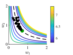
Observe that these global minima lie within connected valleys. For example, in the case of two layers, $\Omega$ corresponds to the hyperbola $w_{2}=\tau/w_{1}$, shown in Fig. 1. Parts of these valleys are sharper than others, and as the theory predicts, GD indeed does not converge to a narrow part of the valley, even when initialized nearby such a global minimum.

Direct computation (see App. III.1) shows that for ${\boldsymbol{w}}\in\Omega$,

Therefore, letting $\boldsymbol{z}=[w_{1}^{-1},w_{2}^{-1},\ldots,w_{m}^{-1}]^{T}$, we can express the Hessian matrix at a global minimum as

Evidently, the Hessian for scalar networks is a rank-one matrix whose (single) nonzero eigenvalue is

To determine the flattest minima, we need to seek for the weights that minimize $\lambda_{\max}\big(\boldsymbol{H}_{\boldsymbol{w}}\big)$. This boils down to solving the constrained optimization problem

As we show in App. III.1, the minimum of this problem is attained when $|w_{1}|=|w_{2}|=\cdots=|w_{m}|$, so that the set of flattest minima is given by

Substituting $|w_{j}|=|\tau|^{1/m}$ into (10), we obtain that the sharpness of the flattest minima is given by

Note that although there exist infinitely many global minima, there are far fewer flattest minima. Specifically, we see that for scalar networks, $\Omega_{0}$ is a discrete set of cardinality $2^{m-1}$. Geometrically speaking, within each connected valley of global minima, we have only one flattest minimum point. This property carries over to the vector case, in the sense that $\Omega_{0}$ is always a set of measure zero within $\Omega$.

This simple exercise of analyzing scalar networks already reveals several interesting properties of flat minima.

1. 1.

   Balancedness. Note from (12) that the flattest minima correspond to networks, which are balanced in the sense that all their layers have the same weight magnitude. This property turns out to break in higher dimensions. However, as we will see, the flattest solutions are always at least nearly balanced, and they exhibit interesting coupling properties.

2. 2.

   Step-size and depth. Observe from (13) that the sharpness of the flattest minima scales roughly linearly with the network’s depth, $m$. Thus, the deeper the network, the smaller the maximal step-size that allows convergence. As we will see, this property persists in higher dimensions. Interestingly, although this behavior is known Nar & Sastry 2018, it has not been previously derived from minima sharpness considerations.

3. 3.

   Valley dimensions. We saw that the Hessian at a global minimum is always rank-1. This implies that at every minimum point, $m-1$ orthogonal directions point into the valley, whereas only one direction points to an ascent slope. We will see that a similar phenomenon occurs also in higher dimensions.

Besides providing a glimpse into the nature of flat minima, the analysis of scalar networks also allows to assess the effectiveness of visualization methods. Particularly, it is common practice to visually compare the sharpness of two minima, ${\boldsymbol{w}}^{(1)}$ and ${\boldsymbol{w}}^{(2)}$, by plotting the loss along the line connecting them Keskar et al. 2016; Jastrzębski et al. 2017. One expects that a flat minimum would appear flatter also along this 1D cross-section. However, our scalar network analysis reveals that this is typically incorrect. Let us first take a two-layer example. Figure 2 shows the loss along the line connecting a flattest minimum point ${\boldsymbol{w}}^{(1)}$ and a sharper one, ${\boldsymbol{w}}^{(2)}$. As can be seen, along this cross-section, both minima have the same sharpness. This is not a result of some particular choice of ${\boldsymbol{w}}^{(2)}$. It turns out that for two-layer scalar networks, the minimas’ sharpness along this cross section are always the same, regardless of how sharp ${\boldsymbol{w}}^{(2)}$ is in practice. For deeper scalar networks, this is not always the case. However, this visualization is still frequently deceiving (see App. III.2).

As we empirically show in Sec. 6, this phenomenon is common also in non-scalar networks with ReLU activations.

We now move on to the general case of non-scalar deep linear networks. To simplify notations, we denote

where a product over an empty set ($q>k$) is defined to be the identity matrix $\boldsymbol{I}$. We make the following assumptions.

1. A1

   The network has the capacity to implement any linear function from $\mathbb{R}^{d_{x}}$ to $\mathbb{R}^{d_{y}}$, namely $\min\{d_{i}\}\geq\min\{d_{x},d_{y}\}$.

2. A2

   The data is white, namely $\hat{\boldsymbol{\Sigma}}_{x}=\boldsymbol{I}$.

We begin by identifying the structure of the Hessian matrix at a global minimum (see App. IV).

Note that $\boldsymbol{\Phi}_{k}$ is a $d_{k}d_{k-1}\times d_{x}d_{y}$ matrix. Therefore, $\boldsymbol{\Phi}$ has only $d_{x}d_{y}$ columns, while its number of rows is the total number of parameters in the net, $N=\sum_{k=1}^{m}d_{k}d_{k-1}$. This shows that for networks with more than one layer, the Hessian at a global minimum is always rank-deficient. For example, if $d_{x}=d_{y}\triangleq d$, then we have from Assumption A1 that $N\geq md^{2}$, so that at any global minimum point, only $d^{2}$ orthogonal directions point to a slope (the Hessian’s rank), while the rest point into the valley of minima. In other words, the dimension of the valley is at least $(1-1/m)$ of the ambient dimension $N$.

In analogy with the scalar setting, we would now like to exploit Lemma 3 for analyzing the set of flattest minima, $\Omega_{0}$. Unfortunately, here it is intractable to derive a closed form expression for $\lambda_{\max}(\boldsymbol{H}_{{\boldsymbol{w}}})$ at an arbitrary minimum point. Yet, our key observation is that it is still possible to determine the minimal value of $\lambda_{\max}(\boldsymbol{H}_{{\boldsymbol{w}}})$ over the set of global minima $\Omega$, as well as its associated eigenvector. That is, we can deduce the sharpness of the flattest minima, without having an explicit expression for the sharpness of arbitrary minima. We elaborate on the proof technique in Sec. 5. Specifically, let $\sigma_{\max}(\boldsymbol{T})$ denote the top singular value of $\boldsymbol{T}$, and let $\boldsymbol{u}$ and $\boldsymbol{v}$ be its corresponding left and right singular vectors. Then we have the following.

This result asserts that the flattest minima become sharper as the number of layers increases (their sharpness grows approximately linearly with $m$ for $m\gg 1$). Since a minimum point ${\boldsymbol{w}}^{*}$ is stable for GD if the step-size satisfies $\eta\leq 2/\lambda_{\max}(\boldsymbol{H}_{{\boldsymbol{w}}^{*}})$, we conclude that the maximal step-size allowing convergence satisfies $\eta_{\max}\leq\frac{1}{m}(\sigma_{\max}(\boldsymbol{T}))^{-2(1-{1}/{m})}$. In other words, the step-size should be taken to be smaller when training deeper models. As mentioned above, this result was also deduced by Nar & Sastry 2018, albeit from different considerations (without explicitly analyzing minima sharpness).

Next, we turn to analyze the flattest minima in terms of the gain that signals experience as they propagate through these networks. For general minimum points, the largest end-to-end gain is $\sigma_{\max}(\boldsymbol{T})$ (corresponding to the input $\boldsymbol{v}$), but the intermediate gain up to layer $k<m$ is unconstrained, as we can always multiply one weight matrix by $\alpha$ and another by $1/\alpha$ without affecting the end-to-end mapping. Flattest minima, however, have special structures. Two questions are thus in place regarding those solutions: (i) What gain does $\boldsymbol{v}$ experience up to layer $k$? (ii) What is the largest gain that any signal can experience up to layer $k$?

Figure 3 illustrates the theorem for six-layer linear networks designed to solve a linear regression problem involving synthetic data (see App. IX for details). Here $\boldsymbol{W}_{j}\in\mathbb{R}^{4\times 4}$ for all layers. The figure depicts eight randomly drawn global minima, four arbitrary and four flattest. The intermediate gain of $\boldsymbol{v}$, to which Theorem 2(i) refers, is marked by red circles. The bound of Theorem 2(ii) is shown as a dotted black line, and the singular values of the partial matrix products are marked by blue dots. As can be seen in Fig. 3(a), the intermediate gains in arbitrary global minimum solutions can be high. However, in the flattest solutions (Fig. 3(b)), the gain that $\boldsymbol{v}$ experiences varies gracefully along the net (as $(\sigma_{\max}(\boldsymbol{T}))^{k/m}$), and the maximal gain of any other signal (highest blue point) is never much larger. Finally, we see that $\boldsymbol{v}$ is indeed one of the singular vectors of the partial product matrix up to any depth (as the red circle coincides with one of the blue points in each layer).

In addition to the intermediate gains, it is of interest to analyze the individual weight matrices. It turns out that in the flattest solutions, the layers exhibit a sort of coupling associated with the signal $\boldsymbol{v}$. Specifically, we have the following.

Remark: From Theorem 2, $\|\boldsymbol{r}_{k}\|=(\sigma_{\max}(\boldsymbol{T}))^{(k-1)/m}$ and $\|\boldsymbol{q}_{k}\|=(\sigma_{\max}(\boldsymbol{T}))^{1-k/m}$.

Theorem 3 indicates that in flattest minimum networks, there forms a distinct path from input to output that is exclusively dedicated to the signal $\boldsymbol{v}$. Specifically, when such a network operates on $\boldsymbol{v}$, the input to each layer is a singular vector of that layer, with singular value $(\sigma_{\max}(\boldsymbol{T}))^{1/m}$. Note that this singular value is not necessarily the maximal one of each layer, but it must exist in all matrices. Now, since the input of each layer is a singular vector, so is its output. Therefore, we have that consecutive layers in the network have a singular vector in common, where a left singular vector of one matrix matches a right singular vector of the next.

We saw that if ${\boldsymbol{w}}\in\Omega_{0}$, then one of the singular values of each weight matrix must equal $(\sigma_{\max}(\boldsymbol{T}))^{1/m}$. One may wonder whether the other direction is also true. As we now show, if the singular value $(\sigma_{\max}(\boldsymbol{T}))^{1/m}$ not only exists, but is also the largest one of each matrix, then the network is necessarily a flattest minimum.

Observe that these cases are not rare, in the sense that they form a set of nonzero measure within $\Omega_{0}$.

Our results in theorems 1-4 hinge on the ability to characterize the flattest minima without having an explicit expression for the top eigenvalue of the Hessian at an arbitrary minimum point. In this section we present an outline of the proof of Theorem 1, which illustrates how we go about this, and lays the basis for the proofs of the other theorems.

Note from (1) that ${\boldsymbol{w}}$ is a concatenation of the vectorizations of the weights matrices $\{\boldsymbol{W}_{j}\}$. That is, denoting ${\boldsymbol{w}}_{j}=\text{vec}\left(\boldsymbol{W}_{j}\right)$, we have that ${\boldsymbol{w}}=[{\boldsymbol{w}}_{1}^{T},{\boldsymbol{w}}_{2}^{T},\ldots,{\boldsymbol{w}}_{m}^{T}]^{T}$. Therefore, the Hessian has the following block structure,

where we use denominator-layout notation. In App. IV we show that if ${\boldsymbol{w}}\in\Omega$, then the $(i,j)$th block is given by

where $\boldsymbol{\Phi}_{i}$ is defined in (16). This implies that we can write $\boldsymbol{H}_{{\boldsymbol{w}}}=2\boldsymbol{\Phi}\boldsymbol{\Phi}^{T}$, where $\boldsymbol{\Phi}=[\boldsymbol{\Phi}_{1}^{T},\boldsymbol{\Phi}_{2}^{T},\ldots,\boldsymbol{\Phi}_{m}^{T}]^{T}$.

To study the maximal eigenvalue of the Hessian, we will be rather looking at the matrix $\hat{\boldsymbol{H}}_{{\boldsymbol{w}}}=2\boldsymbol{\Phi}^{T}\boldsymbol{\Phi}$, whose nonzero eigenvalues coincide with those of $\boldsymbol{H}_{{\boldsymbol{w}}}$. Particularly,

Using the fact that $\|\boldsymbol{\Phi}\boldsymbol{b}\|^{2}=\sum_{k=1}^{m}\|\boldsymbol{\Phi}_{k}\boldsymbol{b}\|^{2}$, together with properties of the Kronecker product (that appears in the definition of $\boldsymbol{\Phi}_{k}$), the right side of (20) can be written as

where $\boldsymbol{b}=\text{vec}\left(\boldsymbol{B}\right)$ (see App. V.3). Obtaining a closed form solution to this optimization problem seems intractable. However, recall that our goal is merely to find the minimal value of $\lambda_{\max}(\boldsymbol{H}_{{\boldsymbol{w}}})$ over ${\boldsymbol{w}}\in\Omega$. This corresponds to a minimax optimization problem over ${\boldsymbol{w}}$ and $\boldsymbol{B}$, where the minimum is taken over ${\boldsymbol{w}}\in\Omega$ and the maximum over $\boldsymbol{B}\in\{\boldsymbol{B}\in\mathbb{R}^{d_{y}\times d_{x}}:\|\boldsymbol{B}\|_{\rm F}=1\}$.

Our solution approach consists of two steps. First, we bound the objective from below using an expression that is independent of ${\boldsymbol{w}}$. Then, we show that there exists a particular choice of ${\boldsymbol{w}}\in\Omega$ that achieves the lower bound. This proves that our bound is in fact the minimax value (i.e. the minimal value of $\lambda_{\max}(\boldsymbol{H}_{{\boldsymbol{w}}})$ over $\Omega$). To this end, we make use of the following lemma (see proof in App. V.1).

This lemma implies that the objective in (21) can be lower-bounded by

Let us write out explicitly two consecutive terms of the outer product,

It is easy to see that the product of the two terms in the middle equals $(\prod_{j=1}^{m}\boldsymbol{W}_{j})^{T}$, which in turn equals $\boldsymbol{T}^{T}$ for global minima. Therefore, if we unwrap the entire outer product, we get $\boldsymbol{T}^{T}$ in between every two appearances of $\boldsymbol{B}\hat{\boldsymbol{\Sigma}}_{x}^{\frac{1}{2}}$, so that (23) reduces to

To recap, we have that if ${\boldsymbol{w}}$ is a global minimum, then $\lambda_{\max}(\boldsymbol{H}_{{\boldsymbol{w}}})\geq\max\nu(\boldsymbol{B})$ s.t. $\|\boldsymbol{B}\|_{\rm F}=1$. For the special case $\hat{\boldsymbol{\Sigma}}_{x}=\boldsymbol{I}$ (Assumption A2), we show in App. V.2 that

We have thus obtained a lower-bound on $\lambda_{\max}(\boldsymbol{H}_{{\boldsymbol{w}}})$, which is independent of ${\boldsymbol{w}}$.

We now determine a particular solution achieving the bound. Denote the SVD of $\boldsymbol{T}$ by $\boldsymbol{U}\boldsymbol{S}\boldsymbol{V}^{T}$ and let ${\boldsymbol{w}}^{*}\in\Omega$ be

Here we slightly abuse the notation $\boldsymbol{S}_{j}^{1/m}$ to denote a $d_{j}\times d_{j-1}$ diagonal matrix whose $k$th diagonal entry is $(\sigma_{k}(\boldsymbol{T}))^{1/m}$, the $k$th largest singular value of $\boldsymbol{T}$. Note that for this particular solution, all the weight matrices have the same set of nonzero singular values, which are precisely the $m$th roots of the singular values of $\boldsymbol{T}$. As we show in App. V.3, for this solution it is rather easy to compute the Hessian’s top eigenvalue, which turns out to equal

Since $\lambda_{\max}(\boldsymbol{H}_{{\boldsymbol{w}}^{*}})$ achieves the lower-bound (26), this bound must be the minimal value of $\lambda_{\max}(\boldsymbol{H}_{{\boldsymbol{w}}})$. We have thus established that

which completes the proof for $\lambda_{\max}(\boldsymbol{H}_{{\boldsymbol{w}}})$. The proof for the corresponding eigenvector can be found in App. V.4.

Two comments are in place. First, note that as a byproduct, we obtained that the solution (27) is a flattest global minimum. This is actually a special case of Theorem 4, which applies also to non-diagonal weight matrices, and to matrices whose singular values do not all coincide with the $m$th roots of the singular values of $\boldsymbol{T}$. Namely, according to Theorem 4, merely requiring that $\sigma_{\max}(\boldsymbol{W}_{k})=(\sigma_{\max}(\boldsymbol{T}))^{1/m}$ for all $k$, already guarantees that a minimum is flattest. Second, although we focused on the case $\hat{\boldsymbol{\Sigma}}_{x}=\boldsymbol{I}$, we conjecture that $\min_{{\boldsymbol{w}}\in\Omega}\lambda_{\max}(\boldsymbol{H}_{{\boldsymbol{w}}})=\max_{\|\boldsymbol{B}\|_{\rm F}=1}\nu(\boldsymbol{B})$ also for arbitrary $\hat{\boldsymbol{\Sigma}}_{x}$. However, in the general setting, there is no closed form solution for the maximization over $\boldsymbol{B}$, so that its study seems to allow no further insight.

Our theoretical results apply to linear networks. Yet, as we now empirically illustrate, they also nicely capture the behavior of nonlinear networks. To show this, we trained fully connected networks with ReLU activation functions to denoise images of handwritten digits. We used the MNIST dataset LeCun 1998 and simulated zero-mean white Gaussian noise of standard deviation $1.25$, where the pixel range of the clean images was $[0,1]$. The input, output, and all intermediate representations had 784 dimensions, so that the total number of parameters was over $600,000\times m$ for an $m$-layer network. We minimized the quadratic loss using SGD without momentum.

We start by demonstrating Theorem 1, which asserts that all minima become sharper as the depth of the network increases. Figure 4 visualizes the result of training networks of different depths using varying step sizes. For each configuration, we measured the top eigenvalue of the Hessian using the power method. Thus, each tile in Fig. 4(a) corresponds to a different trained network, where $\lambda_{\max}(\boldsymbol{H}_{{\boldsymbol{w}}})$ is color-coded and white tiles correspond to non-converged runs. We can see that larger step sizes indeed lead to flatter minima (i.e. more bluish tiles). Also, notice that the maximal step size allowing convergence behaves as $1/m$, in accordance with Theorem 1. Now, for each network depth, we took the lowest measured sharpness, and plotted it against the number of layers in Fig. 4(b). Here we can see that the flattest minima indeed get sharper as the network gets deeper. Particularly, the behavior is roughly linear, as (17) predicts.

In the experiment above, we used identity initialization, as Lemma 1 suggests this should lead to a flat minimum. To verify that this is indeed the case, we repeated the experiment with the initialization of He et al. 2015. As can be seen in Fig. 5(a), in this case SGD indeed converges to sharper minima, and cannot accommodate large step sizes. To further compare these initializations, we plot the loss function during training in Fig. 5(b). We can see that with identity initialization, the loss rapidly convergence already at an early stage, whereas with random initialization it decreases only at later iterations. This shows that identity initialization indeed leads to flatter minima, as Lemma 1 predicts, and that SGD converges faster to flat solutions.

Next, we demonstrate Theorem 2. For the purpose of comparing the properties of sharp and flat solutions, we trained a six layer network for the same denoising problem as above, using two different optimization methods: (i) SGD with a large step size and moderate batch size, a configuration that is known to converge to flat minima Keskar et al. 2016; (ii) Adam Kingma & Ba 2014 with a small step size, which can converge to sharp minima Wu et al. 2018. We ran each method with four different random initializations, and calculated the top eigenvalue of the Hessian at the minimum it converged to. We verified this eigenvalue was indeed significantly smaller (roughly $6\times$) for the minima found by SGD. Now, for each network, we estimated the maximal gain that any signal can experience up to each layer. We did so by optimizing the input so as to maximize the norm of the intermediate signal, where we started from 100 different random initializations and chose the maximum over all runs. These gains are analogous to the top singular values of the partial matrix products in the linear setting. As can be seen in Fig. 6, these gains (blue dots) tend to be high in the sharp solutions, and quite restrained in the flat ones. A similar behavior is seen for the intermediate gains of the signal that experiences the largest end-to-end amplification (red circles). These are analogous to the intermediate gains of the vector $\boldsymbol{v}$ in the linear setting. These behaviors are in accordance with points (ii) and (i) of Theorem 2, respectively.

Finally, we illustrate Lemma 2. For each of the 16 pairs of flat and sharp minima, we evaluated the loss along the line connecting them. The result for one pair is shown in Fig. 7(a) (all 16 pairs showed the same behavior). As can be seen, the flat minimum appears to be sharper than the sharp one along this 1D cross-section. To appreciate how distorted this image is, we also plot in figures 7(d) and 7(e) the loss along the sharpest cross-section of each minimum, which visualizes its true sharpness. This illustration confirms that the interpolation visualization is frequently deceiving also for nonlinear networks in high-dimensional settings.

Gradient descent methods have a bias towards flat minima. In this work, we proved that for linear networks trained with a quadratic loss, these solutions possess unique properties. For example, in flat minima networks, the signal $\boldsymbol{v}$ that experiences the largest gain end-to-end, is amplified as moderately as possible by each layer. Moreover, no other signal can experience a significantly larger gain than $\boldsymbol{v}$ up to an intermediate layer. Finally, these solutions exhibit a coupling between the layers, which forms a distinct path for $\boldsymbol{v}$ from input to output. While our theoretical results apply to linear networks, our experiments show that these properties are also characteristic of nonlinear networks trained in practice.

This research was supported in part by the Technion Ollendorff Minerva Center.

References

• Arora et al. (2018) Arora, S., Cohen, N., and Hazan, E. E. On the optimization of deep networks: Implicit acceleration by overparameterization. In 35th International Conference on Machine Learning, ICML 2018, pp. 372–389. International Machine Learning Society (IMLS), 2018.
• Chaudhari et al. (2019) Chaudhari, P., Choromanska, A., Soatto, S., LeCun, Y., Baldassi, C., Borgs, C., Chayes, J., Sagun, L., and Zecchina, R. Entropy-SGD: Biasing gradient descent into wide valleys. Journal of Statistical Mechanics: Theory and Experiment, 2019(12):124018, 2019.
• Dinh et al. (2017) Dinh, L., Pascanu, R., Bengio, S., and Bengio, Y. Sharp minima can generalize for deep nets. In Proceedings of the 34th International Conference on Machine Learning-Volume 70, pp. 1019–1028. JMLR. org, 2017.
• Du et al. (2018) Du, S. S., Hu, W., and Lee, J. D. Algorithmic regularization in learning deep homogeneous models: Layers are automatically balanced. In Advances in Neural Information Processing Systems, pp. 384–395, 2018.
• Gunasekar et al. (2017) Gunasekar, S., Woodworth, B. E., Bhojanapalli, S., Neyshabur, B., and Srebro, N. Implicit regularization in matrix factorization. In Advances in Neural Information Processing Systems, pp. 6151–6159, 2017.
• Gunasekar et al. (2018a) Gunasekar, S., Lee, J., Soudry, D., and Srebro, N. Characterizing implicit bias in terms of optimization geometry. arXiv preprint arXiv:1802.08246, 2018a.
• Gunasekar et al. (2018b) Gunasekar, S., Lee, J. D., Soudry, D., and Srebro, N. Implicit bias of gradient descent on linear convolutional networks. In Advances in Neural Information Processing Systems, pp. 9461–9471, 2018b.
• He et al. (2015) He, K., Zhang, X., Ren, S., and Sun, J. Delving deep into rectifiers: Surpassing human-level performance on imagenet classification. In Proceedings of the IEEE international conference on computer vision, pp. 1026–1034, 2015.
• Hochreiter & Schmidhuber (1997) Hochreiter, S. and Schmidhuber, J. Flat minima. Neural Computation, 9(1):1–42, 1997.
• Hoffer et al. (2017) Hoffer, E., Hubara, I., and Soudry, D. Train longer, generalize better: closing the generalization gap in large batch training of neural networks. In Advances in Neural Information Processing Systems, pp. 1731–1741, 2017.
• Jastrzębski et al. (2017) Jastrzębski, S., Kenton, Z., Arpit, D., Ballas, N., Fischer, A., Bengio, Y., and Storkey, A. Three factors influencing minima in SGD. arXiv preprint arXiv:1711.04623, 2017.
• Ji & Telgarsky (2019) Ji, Z. and Telgarsky, M. J. Gradient descent aligns the layers of deep linear networks. In 7th International Conference on Learning Representations, ICLR 2019, 2019.
• Keskar et al. (2016) Keskar, N. S., Mudigere, D., Nocedal, J., Smelyanskiy, M., and Tang, P. T. P. On large-batch training for deep learning: Generalization gap and sharp minima. arXiv preprint arXiv:1609.04836, 2016.
• Kingma & Ba (2014) Kingma, D. P. and Ba, J. Adam: A method for stochastic optimization. arXiv preprint arXiv:1412.6980, 2014.
• LeCun (1998) LeCun, Y. The MNIST database of handwritten digits. 1998.
• Li et al. (2018) Li, H., Xu, Z., Taylor, G., Studer, C., and Goldstein, T. Visualizing the loss landscape of neural nets. In Advances in Neural Information Processing Systems, pp. 6389–6399, 2018.
• Lyu & Li (2020) Lyu, K. and Li, J. Gradient descent maximizes the margin of homogeneous neural networks. In International Conference on Learning Representations, 2020.
• Masters & Luschi (2018) Masters, D. and Luschi, C. Revisiting small batch training for deep neural networks. arXiv preprint arXiv:1804.07612, 2018.
• Morgan & Bourlard (1990) Morgan, N. and Bourlard, H. Generalization and parameter estimation in feedforward nets: Some experiments. In Advances in neural information processing systems, pp. 630–637, 1990.
• Nar & Sastry (2018) Nar, K. and Sastry, S. Step size matters in deep learning. In Advances in Neural Information Processing Systems, pp. 3436–3444, 2018.
• Neyshabur et al. (2014) Neyshabur, B., Tomioka, R., and Srebro, N. In search of the real inductive bias: On the role of implicit regularization in deep learning. arXiv preprint arXiv:1412.6614, 2014.
• Neyshabur et al. (2017) Neyshabur, B., Bhojanapalli, S., McAllester, D., and Srebro, N. Exploring generalization in deep learning. In Advances in Neural Information Processing Systems, pp. 5947–5956, 2017.
• Simsekli et al. (2019) Simsekli, U., Sagun, L., and Gurbuzbalaban, M. A tail-index analysis of stochastic gradient noise in deep neural networks. arXiv preprint arXiv:1901.06053, 2019.
• Smith & Le (2017) Smith, S. L. and Le, Q. V. A bayesian perspective on generalization and stochastic gradient descent. arXiv preprint arXiv:1710.06451, 2017.
• Soudry et al. (2018) Soudry, D., Hoffer, E., Nacson, M. S., Gunasekar, S., and Srebro, N. The implicit bias of gradient descent on separable data. The Journal of Machine Learning Research, 19(1):2822–2878, 2018.
• Strand (1974) Strand, O. N. Theory and methods related to the singular-function expansion and landweber’s iteration for integral equations of the first kind. SIAM Journal on Numerical Analysis, 11(4):798–825, 1974.
• Wu et al. (2018) Wu, L., Ma, C., and Weinan, E. How SGD selects the global minima in over-parameterized learning: A dynamical stability perspective. In Advances in Neural Information Processing Systems, pp. 8279–8288, 2018.
• Wu et al. (2019) Wu, X., Dobriban, E., Ren, T., Wu, S., Li, Z., Gunasekar, S., Ward, R., and Liu, Q. Implicit regularization of normalization methods. arXiv preprint arXiv:1911.07956, 2019.
• Zhang et al. (2018) Zhang, H., Dauphin, Y. N., and Ma, T. Fixup initialization: Residual learning without normalization. In International Conference on Learning Representations, 2018.
Unique Properties of Flat Minima in Deep Networks:
Supplementary Material
Appendix I Stability of Minima
It is well know that for a β\beta-smooth function that is bounded from below, GD with constant step size 0<η<2/β0<\eta<2/\beta converges to a stationary point. A twice continuously differentiable function ff is β\beta-smooth if and only if λmax​(∇2f​(𝒘))≤β\lambda_{\max}(\nabla^{2}f({\boldsymbol{w}}))\leq\beta for every point 𝒘∈ℝN{\boldsymbol{w}}\in\mathbb{R}^{N}. Hence, convergence to a stationary point is guaranteed if λmax​(∇2f​(𝒘))≤2/η\lambda_{\max}(\nabla^{2}f({\boldsymbol{w}}))\leq 2/\eta for all 𝒘∈ℝN{\boldsymbol{w}}\in\mathbb{R}^{N}. This seemingly stringent global requirement can in fact also be replaced by a local one, as shown by Wu et al. 2018. Specifically, they use the following.
Definition S1.
Let 𝐰∗{\boldsymbol{w}}^{*} be a stationary point of ff. Consider the linearized dynamical system of GD, namely
𝒘k+1=𝒘k−η​∇2f​(𝒘∗)​(𝒘k−𝒘∗).{\boldsymbol{w}}_{k+1}={\boldsymbol{w}}_{k}-\eta\nabla^{2}f({\boldsymbol{w}}^{*})({\boldsymbol{w}}_{k}-{\boldsymbol{w}}^{*}). (S1)
Then 𝐰∗{\boldsymbol{w}}^{*} is said to be linearly stable if there exists a constant C∈ℝC\in\mathbb{R}, such that ‖𝐰k‖≤C⁡‖𝐰0‖\left\lVert{\boldsymbol{w}}_{k}\right\rVert\leq C\left\lVert{\boldsymbol{w}}_{0}\right\rVert for all k>0k>0.
In other words, 𝒘∗{\boldsymbol{w}}^{*} is linearly stable if once we have arrived near this critical point, we stay around it. In their paper, Wu et al. 2018 show that 𝒘∗{\boldsymbol{w}}^{*} is a linearly stable minimizer if
λmax​((𝑰−η​∇2f​(𝒘∗))2)≤1.\lambda_{\max}\left(\big(\boldsymbol{I}-\eta\nabla^{2}f({\boldsymbol{w}}^{*})\big)^{2}\right)\leq 1. (S2)
Note that for all i∈{1,…,N}i\in\{1,\ldots,N\}
λi​((𝑰−η​∇2f​(𝒘∗))2)\displaystyle\lambda_{i}\left(\big(\boldsymbol{I}-\eta\nabla^{2}f({\boldsymbol{w}}^{*})\big)^{2}\right) =λi2​(𝑰−η​∇2f​(𝒘∗))\displaystyle=\lambda^{2}_{i}\left(\boldsymbol{I}-\eta\nabla^{2}f({\boldsymbol{w}}^{*})\right)
=(1−η​λi​(∇2f​(𝒘∗)))2\displaystyle=\left(1-\eta\lambda_{i}\left(\nabla^{2}f({\boldsymbol{w}}^{*})\right)\right)^{2}
=1−η​λi​(∇2f​(𝒘∗))​(2−η​λi​(∇2f​(𝒘∗))),\displaystyle=1-\eta\lambda_{i}\left(\nabla^{2}f({\boldsymbol{w}}^{*})\right)\left(2-\eta\lambda_{i}\left(\nabla^{2}f({\boldsymbol{w}}^{*})\right)\right), (S3)
where λi\lambda_{i} is the iith largest eigenvalue. Since η\eta and {λi}\{\lambda_{i}\} are all nonnegative, it follows that (S2) is equivalent to
λmax​(∇2f​(𝒘∗))≤2η.\lambda_{\max}\left(\nabla^{2}f({\boldsymbol{w}}^{*})\right)\leq\frac{2}{\eta}. (S4)
This results asserts that flat minima are stable solutions for GD. In their paper, they also provide a similar result for stochastic GD (SGD), which shows that the sharpness of a minimum should increase to ensure stability for SGD as well.
Appendix II Proof of Lemma 1
Nar & Sastry 2018 showed that under the Lemma’s conditions, the weight matrices converge at a linear rate to 𝑾i=𝑻1m\boldsymbol{W}_{i}=\boldsymbol{T}^{\frac{1}{m}} for all ii. According to our Theorem 4, this solution is a flattest minimum, thus demonstrating (i​iii).
Arora et al. 2018 showed that gradient flow (GF) satisfies
𝑾i​(t)​𝑾iT​(t)=𝑾i+1T​(t)​𝑾i+1​(t),∀t≥0\boldsymbol{W}_{i}(t)\boldsymbol{W}^{T}_{i}(t)=\boldsymbol{W}^{T}_{i+1}(t)\boldsymbol{W}_{i+1}(t),\quad\forall t\geq 0 (S5)
in our setting. Denoting the SVD of 𝑾i​(t)\boldsymbol{W}_{i}(t) by 𝑼i​(t)​𝑺i​(t)​𝑽iT​(t)\boldsymbol{U}_{i}(t)\boldsymbol{S}_{i}(t)\boldsymbol{V}^{T}_{i}(t), we thus have that 𝑼i​(t)​𝑺i2​(t)​𝑼iT​(t)=𝑽i+1​(t)​𝑺i+12​(t)​𝑽i+1T​(t)\boldsymbol{U}_{i}(t)\boldsymbol{S}^{2}_{i}(t)\boldsymbol{U}^{T}_{i}(t)=\boldsymbol{V}_{i+1}(t)\boldsymbol{S}^{2}_{i+1}(t)\boldsymbol{V}^{T}_{i+1}(t), which implies that11 1 The SVD can be non-unique, however there necessarily exists a decomposition satisfying 𝑼i​(t)=𝑽i+1​(t)\boldsymbol{U}_{i}(t)=\boldsymbol{V}_{i+1}(t).
𝑼i​(t)=𝑽i+1​(t),𝑺i​(t)=𝑺i+1​(t),∀t≥0.\boldsymbol{U}_{i}(t)=\boldsymbol{V}_{i+1}(t),\quad\boldsymbol{S}_{i}(t)=\boldsymbol{S}_{i+1}(t),\quad\forall t\geq 0. (S6)
Assume that GF converges to a global minimimum and let 𝑼​𝑺​𝑽T\boldsymbol{U}\boldsymbol{S}\boldsymbol{V}^{T} denote the SVD of 𝑻\boldsymbol{T}. Since {𝑺i​(t)}i=1m\{\boldsymbol{S}_{i}(t)\}_{i=1}^{m} are identical, they converge to the same limit, 𝑺¯\bar{\boldsymbol{S}}. Let 𝑾i=𝑼i​𝑺¯​𝑽iT\boldsymbol{W}_{i}=\boldsymbol{U}_{i}\bar{\boldsymbol{S}}\boldsymbol{V}_{i}^{T} denote the limit of 𝑾i​(t)\boldsymbol{W}_{i}(t). Then, from (S6), we have that 𝑽i+1T​𝑼i=𝑰\boldsymbol{V}_{i+1}^{T}\boldsymbol{U}_{i}=\boldsymbol{I} for all ii. Consequently,
𝑾m𝑾m−1⋯𝑾1=𝑼m𝑺¯m𝑽T1.\boldsymbol{W}_{m}\boldsymbol{W}_{m-1}\cdots\boldsymbol{W}_{1}=\boldsymbol{U}_{m}\bar{\boldsymbol{S}}^{m}\boldsymbol{V}^{T}_{1}. (S7)
But since the left hand side equals 𝑻\boldsymbol{T} by assumption, the right hand side must coincide with the SVD of 𝑻\boldsymbol{T}. This means that 𝑺¯=𝑺1m\bar{\boldsymbol{S}}=\boldsymbol{S}^{\frac{1}{m}}. Again, by Theorem 4, this is a flattest minimum, thus demonstrating (ii).
Appendix III Scalar Networks
III.1 The Set of Flattest Minima
As mentioned in the main text, in the scalar case, the end-to-end function f𝒘​(x)f_{\boldsymbol{w}}(x) implemented by the network is given by
f𝒘​(x)=∏j=1mwj​x,f_{\boldsymbol{w}}(x)=\prod_{j=1}^{m}w_{j}x, (S8)
where 𝒘=[w1,w2,…,wm]T{\boldsymbol{w}}=[w_{1},w_{2},\ldots,w_{m}]^{T}. In our analysis we consider a quadratic loss function, i.e.
ℓ⁡(𝒘)=𝔼^​[(y−f𝒘​(x))2].\ell({\boldsymbol{w}})=\hat{\mathbb{E}}\left[\big(y-f_{\boldsymbol{w}}(x)\big)^{2}\right]. (S9)
Our goal is to characterize the set of flattest minima of the loss w.r.t. 𝒘{\boldsymbol{w}}. It is well known that the optimal coefficient for linear estimation is given by
τ=σ^x​yσ^x2,\tau=\frac{\hat{\sigma}_{xy}}{\hat{\sigma}_{x}^{2}}, (S10)
where σ^x2=E⁡[x2]\hat{\sigma}_{x}^{2}=\mathrm{E}[x^{2}] is the empirical second-order moment of xx, and σ^x​y=E⁡[x​y]\hat{\sigma}_{xy}=\mathrm{E}[xy] is the empirical cross second-order moment between xx and yy. Therefore, at any global minimum of ℓ⁡(𝒘)\ell({\boldsymbol{w}}), we have
∏j=1mwj=τ.\prod_{j=1}^{m}w_{j}=\tau. (S11)
To compute the Hessian matrix of ℓ⁡(𝒘)\ell({\boldsymbol{w}}), we first calculate the partial derivative w.r.t. wkw_{k},
∂∂wk​ℓ​(𝒘)\displaystyle\frac{\partial}{\partial w_{k}}\ell({\boldsymbol{w}}) =∂∂wk​𝔼^​[(y−f𝒘​(x))2]=−2​𝔼^​[(y−f𝒘​(x))​∂∂wk​f𝒘​(x)]\displaystyle=\frac{\partial}{\partial w_{k}}\hat{\mathbb{E}}\left[\big(y-f_{\boldsymbol{w}}(x)\big)^{2}\right]=-2\hat{\mathbb{E}}\left[\big(y-f_{\boldsymbol{w}}(x)\big)\frac{\partial}{\partial w_{k}}f_{\boldsymbol{w}}(x)\right]
=−2​𝔼^​[(y−∏j=1mwj​x)​∏j≠kwj​x]=2​(σ^x2​∏j=1mwj−σ^x​y)​∏j≠kwj\displaystyle=-2\hat{\mathbb{E}}\left[\Big(y-\prod_{j=1}^{m}w_{j}x\Big)\prod_{j\neq k}w_{j}x\right]=2\Big(\hat{\sigma}_{x}^{2}\prod_{j=1}^{m}w_{j}-\hat{\sigma}_{xy}\Big)\prod_{j\neq k}w_{j} (S12)
We now complete the derivation by differentiating (III.1) w.r.t. wqw_{q},
∂2∂wq​∂wk​ℓ​(𝒘)\displaystyle\frac{\partial^{2}}{\partial w_{q}\partial w_{k}}\ell({\boldsymbol{w}}) =∂∂wq​[2​(σ^x2​∏j=1mwj−σ^x​y)​∏j≠kwj]\displaystyle=\frac{\partial}{\partial w_{q}}\left[2\Big(\hat{\sigma}_{x}^{2}\prod_{j=1}^{m}w_{j}-\hat{\sigma}_{xy}\Big)\prod_{j\neq k}w_{j}\right]
=2​∏j≠kwj​∂∂wq​(σ^x2​∏j=1mwj−σ^x​y)+2​(σ^x2​∏j=1mwj−σ^x​y)​∂∂wq​∏j≠kwj.\displaystyle=2\prod_{j\neq k}w_{j}\frac{\partial}{\partial w_{q}}\Big(\hat{\sigma}_{x}^{2}\prod_{j=1}^{m}w_{j}-\hat{\sigma}_{xy}\Big)+2\Big(\hat{\sigma}_{x}^{2}\prod_{j=1}^{m}w_{j}-\hat{\sigma}_{xy}\Big)\frac{\partial}{\partial w_{q}}\prod_{j\neq k}w_{j}. (S13)
Eq. (S11) asserts that σ^x2​∏j=1mwj−σ^x​y=0\hat{\sigma}_{x}^{2}\prod_{j=1}^{m}w_{j}-\hat{\sigma}_{xy}=0 at global minima, therefore the second term in (III.1) vanishes, and we obtain
∂2∂wq​∂wk​L​(𝒘)=2​∏j≠kwj​∂∂wq​(σ^x2​∏j=1mwj−σ^x​y)=2​σ^x2​(∏j≠kwj)​(∏j≠qwj).\frac{\partial^{2}}{\partial w_{q}\partial w_{k}}L({\boldsymbol{w}})=2\prod_{j\neq k}w_{j}\frac{\partial}{\partial w_{q}}\Big(\hat{\sigma}_{x}^{2}\prod_{j=1}^{m}w_{j}-\hat{\sigma}_{xy}\Big)=2\hat{\sigma}_{x}^{2}\Big(\prod_{j\neq k}w_{j}\Big)\Big(\prod_{j\neq q}w_{j}\Big). (S14)
Hence, using (S10), we can express the elements of the Hessian matrix 𝑯𝒘\boldsymbol{H}_{\boldsymbol{w}} as
(𝑯𝒘)k,q=2​σ^x2​τ2​1wk​wq.\big(\boldsymbol{H}_{\boldsymbol{w}}\big)_{k,q}=2\hat{\sigma}_{x}^{2}\tau^{2}\frac{1}{w_{k}w_{q}}. (S15)
Let us define the vector 𝒛=[w1−1,w2−1,…,wm−1]T\boldsymbol{z}=[w_{1}^{-1},w_{2}^{-1},\ldots,w_{m}^{-1}]^{T}, then the Hessian matrix can be equivalently written as
𝑯𝒘=2​σ^x2​τ2​𝒛​𝒛T.\boldsymbol{H}_{\boldsymbol{w}}=2\hat{\sigma}_{x}^{2}\tau^{2}\boldsymbol{z}\boldsymbol{z}^{T}. (S16)
This shows that the Hessian is a rank one matrix, which implies that it has only one nonzero eigenvalue, with a corresponding eigenvector 𝒛\boldsymbol{z}. Therefore,
λmax​(𝑯𝒘)​𝒛=𝑯𝒘​𝒛=2​σ^x2​(τ)2​𝒛​𝒛T​𝒛=2​σ^x2​(τ)2​‖𝒛‖2​𝒛,\lambda_{\max}\big(\boldsymbol{H}_{\boldsymbol{w}}\big)\boldsymbol{z}=\boldsymbol{H}_{\boldsymbol{w}}\boldsymbol{z}=2\hat{\sigma}_{x}^{2}\big(\tau\big)^{2}\boldsymbol{z}\boldsymbol{z}^{T}\boldsymbol{z}=2\hat{\sigma}_{x}^{2}\big(\tau\big)^{2}\left\lVert\boldsymbol{z}\right\rVert^{2}\boldsymbol{z}, (S17)
so that the eigenvalue is given by
λmax​(𝑯𝒘)=2​σ^x2​τ2​‖𝒛‖2=2​σ^x2​τ2​∑j=1m1wj2.\lambda_{\max}\big(\boldsymbol{H}_{\boldsymbol{w}}\big)=2\hat{\sigma}_{x}^{2}\tau^{2}\|\boldsymbol{z}\|^{2}=2\hat{\sigma}_{x}^{2}\tau^{2}\sum_{j=1}^{m}\frac{1}{w_{j}^{2}}. (S18)
To determine the sharpness of the flattest minima, we need to solve the problem
min𝒘∈ℝm⁡λmax​(𝑯𝒘)s.t.∏j=1mwj=τ.\min_{{\boldsymbol{w}}\in\mathbb{R}^{m}}\ \lambda_{\max}\big(\boldsymbol{H}_{\boldsymbol{w}}\big)\qquad\text{s.t.}\qquad\prod_{j=1}^{m}w_{j}=\tau. (S19)
By the inequality of the arithmetic and geometric means, we have that for any feasible point 𝒘{\boldsymbol{w}}
∑j=1m1wj2≥m×(∏j=1m1wj2)1m=m×τ−2m.\sum_{j=1}^{m}\frac{1}{w_{j}^{2}}\geq m\times\Bigg(\prod_{j=1}^{m}\frac{1}{w_{j}^{2}}\Bigg)^{\frac{1}{m}}=m\times\tau^{-\frac{2}{m}}. (S20)
Therefore, for all feasible points,
λmax​(𝑯𝒘)≥2​m​σ^x2​τ2​(1−1m).\lambda_{\max}\big(\boldsymbol{H}_{\boldsymbol{w}}\big)\geq 2m\hat{\sigma}_{x}^{2}\tau^{2(1-\frac{1}{m})}. (S21)
On the other hand, this inequality can be achieved by setting |w1|=|w2|=⋯=|wm||w_{1}|=|w_{2}|=\cdots=|w_{m}|. This shows that the right-hand-side is precisely the sharpness of the flattest minimum, so that
Ω0={𝒘∈ℝm:∏j=1msgn(wj)=sgn(τ)and|wj|=|τ|m∀j}.\Omega_{0}=\Big\{{\boldsymbol{w}}\in\mathbb{R}^{m}\ :\prod_{j=1}^{m}\text{sgn}(w_{j})=\text{sgn}\big(\tau\big)\quad\text{and}\quad\ |w_{j}|=\sqrt[m]{|\tau|}\quad\forall j\Big\}. (S22)
III.2 Proof of Lemma 2
In this section we examine the behavior of the loss function on a line connecting two minima.
Claim S1.
Assume that τ>0\tau>0 and let 𝐰(1){\boldsymbol{w}}^{(1)} and 𝐰(2){\boldsymbol{w}}^{(2)} be minimizers of the objective (S9) in ℝ+m\mathbb{R}^{m}_{+}. Then, along the line connecting 𝐰(1){\boldsymbol{w}}^{(1)} and 𝐰(2){\boldsymbol{w}}^{(2)}, the loss function will appear sharper around 𝐰(1){\boldsymbol{w}}^{(1)} than around 𝐰(2){\boldsymbol{w}}^{(2)} if
∑i=1mwi(2)wi(1)>∑i=1mwi(1)wi(2).\sum_{i=1}^{m}\frac{w_{i}^{(2)}}{w_{i}^{(1)}}>\sum_{i=1}^{m}\frac{w_{i}^{(1)}}{w_{i}^{(2)}}. (S23)
Proof.
The direction vector of the connecting line is 𝜶=(𝒘(1)−𝒘(2))/‖𝒘(1)−𝒘(2)‖\boldsymbol{\alpha}=({\boldsymbol{w}}^{(1)}-{\boldsymbol{w}}^{(2)})/\|{\boldsymbol{w}}^{(1)}-{\boldsymbol{w}}^{(2)}\|. Along this direction, the behavior of the loss function around 𝒘(i){\boldsymbol{w}}^{(i)} is given by
ℓ(𝒘(i)+η𝜶)≈ℓ(𝒘(i))+η𝜶T∇ℓ(𝒘(i))+η22𝜶T𝑯(𝒘(i))𝜶.\ell({\boldsymbol{w}}^{(i)}+\eta\boldsymbol{\alpha})\approx\ell({\boldsymbol{w}}^{(i)})+\eta\boldsymbol{\alpha}^{T}\nabla\ell({\boldsymbol{w}}^{(i)})+\frac{\eta^{2}}{2}\boldsymbol{\alpha}^{T}\boldsymbol{H}({\boldsymbol{w}}^{(i)})\boldsymbol{\alpha}. (S24)
Since ∇ℓ​(𝒘(1))=∇ℓ​(𝒘(2))=𝟎\nabla\ell({\boldsymbol{w}}^{(1)})=\nabla\ell({\boldsymbol{w}}^{(2)})=\boldsymbol{0} and ℓ⁡(𝒘(1))=ℓ⁡(𝒘(2))\ell({\boldsymbol{w}}^{(1)})=\ell({\boldsymbol{w}}^{(2)}), the loss function will appear sharper around 𝒘(1){\boldsymbol{w}}^{(1)} than around 𝒘(2){\boldsymbol{w}}^{(2)}, if 𝜶T​𝑯​(𝒘(1))​𝜶>𝜶T​𝑯​(𝒘(2))​𝜶\boldsymbol{\alpha}^{T}\boldsymbol{H}({\boldsymbol{w}}^{(1)})\boldsymbol{\alpha}>\boldsymbol{\alpha}^{T}\boldsymbol{H}({\boldsymbol{w}}^{(2)})\boldsymbol{\alpha}. From (S16), this condition is equivalent to ‖𝜶T​𝒛(1)‖2>‖𝜶T​𝒛(2)‖2\|\boldsymbol{\alpha}^{T}\boldsymbol{z}^{(1)}\|^{2}>\|\boldsymbol{\alpha}^{T}\boldsymbol{z}^{(2)}\|^{2}, or more explicitly,
((𝒘(1)−𝒘(2))T​𝒛(1))2>((𝒘(1)−𝒘(2))T​𝒛(2))2.\left(\left({\boldsymbol{w}}^{(1)}-{\boldsymbol{w}}^{(2)}\right)^{T}\boldsymbol{z}^{(1)}\right)^{2}>\left(\left({\boldsymbol{w}}^{(1)}-{\boldsymbol{w}}^{(2)}\right)^{T}\boldsymbol{z}^{(2)}\right)^{2}. (S25)
Since 𝒛=[w1−1,w2−1,…,wm−1]T\boldsymbol{z}=[w_{1}^{-1},w_{2}^{-1},\ldots,w_{m}^{-1}]^{T}, this inequality can be written as