∎
Entropy-stable, high-order summation-by-parts discretizations without interface penaltiesThanks: This is a pre-print of an article published in The Journal of Scientific Computing. The final authenticated version is available online at: https://doi.org/10.1007/s10915-020-01154-8
Abstract
The paper presents high-order accurate, energy-, and entropy-stable discretizations constructed from summation-by-parts (SBP) operators. Notably, the discretizations assemble global SBP operators and use continuous solutions, unlike previous efforts that use discontinuous SBP discretizations. Derivative-based dissipation and local-projection stabilization (LPS) are investigated as options for stabilizing the baseline discretization. These stabilizations are equal up to a multiplicative constant in one dimension, but only LPS remains well conditioned for general, multidimensional SBP operators. Furthermore, LPS is able to take advantage of the additional nodes required by degree diagonal-norms, resulting in an element-local stabilization with a bounded spectral radius. An entropy-stable version of LPS is easily obtained by applying the projection on the entropy variables. Numerical experiments with the linear-advection and Euler equations demonstrate the accuracy, efficiency, and robustness of the stabilized discretizations, and the continuous approach compares favorably with the more common discontinuous SBP methods.
Keywords:
summation-by-parts entropy stable stabilizationMSC
65M06 65M60 65M70 65M121 Introduction
High-order discretizations have been put forward as a possible means of improving the efficiency of computational fluid dynamics (CFD) simulations. The arguments in favor of high-order discretizations include both improved accuracy-per-degree-of-freedom as well as better cache usage on current and future architectures. Despite these potential advantages, the use of high-order CFD remains uncommon in industry. Mesh generation of curved elements is one bottleneck facing high-order methods, but the issue I focus on here is robustness: high-order discretizations have inherently less numerical dissipation, which makes them prone to instabilities, particularly for under-resolved flows.
Entropy stability offers one promising avenue for constructing robust, high-order CFD methods. This is not a new idea. For example, over thirty years ago, Hughes et al. Hughes1986new presented a finite-element discretization of the compressible Navier-Stokes equations that satisfied the second-law of thermodynamics. And in 1999, Barth Barth1999numerical extended this work to cover Galerkin-least-squares stabilizations and discontinuous Galerkin (DG) schemes. However, these early examples make the assumption that the integrations present in the finite-element semi-linear forms are exact. Exact integration is not possible, in general, for the Euler and Navier-Stokes equations, so these schemes must rely on potentially costly “over-integration” in practice. Even then, the discrete schemes are not provably stable and may fail.
In light of the above, there has been growing interest in semi-discrete and fully-discrete high-order schemes that are provably entropy stable. Fisher’s thesis Fisher2012thesis represented a seminal contribution in this direction — see also Fisher2013discretely and Fisher2013high. He showed that summation-by-parts (SBP) finite difference methods could be combined with entropy-conservative flux functions Tadmor1987entropy; Tadmor2003entropy; Ismail2009affordable; Chandrashekar2015kinetic to produce high-order entropy-stable schemes. This was later extended to tensor-product spectral-element methods Carpenter2014entropy; Parsani2016entropy that also possess the summation-by-parts property Gassner2013skew. Subsequently, SBP operators were generalized to simplex elements in multiSBP and later used to construct entropy-stable discretizations on triangular and tetrahedral grids Chen2017entropy; Crean2018entropy.
My objective in this paper is to extend the entropy-stable SBP-framework to continuous-Galerkin type discretizations. Previous entropy-stable SBP discretizations have focused on discontinuous-Galerkin (DG)-type methods; even the finite-difference methods in Fisher2012thesis, Fisher2013discretely, and Fisher2013high used numerical flux functions embedded in penalty terms to couple blocks in multi-block grids. My motivation for considering continuous SBP (C-SBP) discretizations, which were first proposed in multiSBP, is to reduce the computational cost of the residual evaluations by eliminating the interface penalties.
Stabilization is arguably the principal challenge in adapting the entropy-stable framework to C-SBP discretizations. It is well-known that continuous Galkerin finite-element methods produce oscillatory solutions for hyperbolic partial-differential equations (PDEs) and require stabilization; examples of stabilizations include stream-line upwind Petrov-Galerkin (SUPG) Brooks1982streamline, Galerkin-least-squares (GLS) Hughes1989gls, variational multiscale Hughes1995multiscale, edge stabilization Douglas1976interior, and local-projection stabilization (LPS) Becker2001finite, to name a few.
Each stabilization that has been proposed has advantages and disadvantages. Therefore, in order to identify a suitable choice for an entropy-stable C-SBP scheme, a list of desired properties is useful.
- Entropy stable:
-
It must be possible to make the stabilization provably entropy stable, at least at the semi-discrete level. This rules out SUPG as a potential candidate, as well as other non-symmetric stabilizations.
- Well conditioned:
-
The stabilization should have a spectral radius that is comparable to D-SBP discretizations. For example, edge stabilization based on jumps in the gradient Douglas1976interior; Burman2004edge; Burman2006continuous can be made entropy stable, but numerical experiments Crean2016investigation indicate that it has poor conditioning, especially as the discretization order increases. Numerical experiments (not reported here) also suggest that GLS has poor conditioning.
- Element local:
-
I would like the stabilization to have a stencil that matches the stencil of the (unstabilized) discretization. This requirement reduces parallel communication and memory requirements for the Jacobian. It also greatly simplifies algorithmic differentiation, since coloring can be performed at the element level. Edge stabilization and LPS are not element local, in general, while SUPG and GLS are.
To the best of my knowledge, no stabilization meets all the requirements listed above, so a compromise is necessary. The solution that I advocate here is to sacrifice optimal approximation accuracy by increasing the number of nodes necessary for a degree basis. The additional degrees of freedom enable the creation of an entropy-stable, well-conditioned LPS to be applied at the element level. While sacrificing optimal approximation may be unpalatable to some, I believe this is an attractive holistic solution, since diagonal-norm SBP operators also typically require more nodes than a degree basis multiSBP; Fernandez2017simultaneous.
I begin below by describing the C-SBP discretization and its stabilization in the context of the constant-coefficient, linear advection equation; see Section 2. In Section 3, I review the entropy conservation of (unstabilized) C-SBP discretizations in the context of the Euler equations and show how LPS can be used to create an entropy-stable stabilization. I detail the SBP and LPS operators and their construction in Section 4. I verify the discretizations in Section 5 by presenting some numerical experiments, and I conclude with a summary and discussion in Section 6.
2 Stabilization of continuous SBP discretizations: linear advection
In this section, I use the constant-coefficient linear advection equation to present the key ideas behind the proposed stabilization. As discussed in the introduction, these ideas are i) sacrificing optimal-polynomial approximation to achieve a localized stabilization, and ii) using a local-projection-based stabilization.
While most readers will be interested in more useful PDEs, such as the Euler or Navier-Stokes equations, I begin with the linear-advection equation because it avoids complications that I believe would obscure an intuitive understanding of the stabilization. It also provides a simple context to review C-SBP discretitzations.
2.1 The unstabilized SBP discretization in one-dimension
Consider the one-dimensional, constant-coefficient advection equation on a unit periodic domain :
| (1) | ||||||
where is the advection velocity and is a source.
Let the domain be divided into the mesh
of elements of uniform size . The SBP discretization that we consider in this section is a spectral-collocation method using Legendre-Gauss-Lobbato (LGL) nodes, where the solution is stored at LGL quadrature nodes on each element . See Figure 1 for an example of the mesh and the quadrature points.

Remark 1
A conventional spectral-collocation method based on LGL nodes uses collocation points on each element, where is the degree of the polynomial basis. In this work we use , which is more like a finite-difference operator. We will motivate this decision later in Section 2.2.2.
The global solution is denoted by the vector , where the number of degrees of freedom in this example is ; for those more familiar with discontinuous SBP discretizations, the solution here is not multivalued at the element interfaces.
In order to manipulate the global solution at the element-level, we need to define restriction and prolongation operators. To this end, consider a global node with index that coincides with the local index on element ; again, see Figure 1. Then the th entry of the restriction matrix is unity: . For example, assuming the nodes are ordered sequentially, both on each element and globally, the restriction operator for element in Figure 1 is
The prolongation operator on element is simply the transpose of .
Next, I introduce a degree diagonal-norm SBP operator on the LGL nodes in the reference space ; see Gassner2013 for the case and DCDRF2014 for the more general case. Briefly, is a finite-difference operator that exactly differentiates degree polynomials at the nodes. Furthermore, is a diagonal matrix with positive entries along its diagonal, and the symmetric part of satisfies . I will review the multidimensional SBP definition in Section 4.
Using the restriction operators and the matrices and , one can define an SBP operator that acts on the global degrees of freedom:
| where | |||
| (2) | |||
The fact that defines a degree SBP operator at the nodes on was established in multiSBP.
Remark 2
For the case , and define the stiffness and lumped-mass matrices for a spectral collocation scheme.
Remark 3
For the periodic case under consideration, the symmetric part of is zero:
since the and values in from adjacent elements cancel at the common node. This will be an important property that we will also need for entropy conservation in the multidimensional case in Section 3.
2.1.1 Strong-form discretization
Using the global operator , the SBP semi-discretization of (1) is given by
| (3) |
where is the evaluation of at the nodes. The truncation error, energy stability, and conservative nature of (3) follow from the properties of the SBP operator ; see, for example, the reviews Svard2014 and Fernandez2014.
2.1.2 Weak-form discretization
I will now show that (3) is also a discretization of the weak formulation of the constant-coefficient linear advection equation. Let denote the Hilbert space of periodic functions on with bounded derivatives. Then the weak formulation of (1) is obtained by multiplying the PDE by an arbitrary , integrating over the domain, and applying integration by parts; that is, find such that
| (4) |
To mimic (4) in the discrete case, let denote the value of a test function evaluated at the nodes of . Then, left-multiplying (3) by we find
| (5) |
where I have used the SBP property , and the fact that for the periodic problem under consideration.
There is an obvious structural similarity between (4) and (5); however, the similarity between the two weak forms is more than qualitative. Since is a diagonal-norm SBP first-derivative operator, it follows that and the nodes define a degree quadrature rule, and approximates the weak derivative Hicken2013quad; multiSBP:
Thus, beyond mimicking the structure of (4), each term in (5) is actually a high-order approximation of the corresponding term in the continuous equation.
Remark 4
While many discretizations may approximate (4) to high-order, the strength of SBP discretizations is that they also mimic integration by parts exactly; that is, few schemes also satisfy the SBP property, , which is valuable in proving stability.
2.1.3 Element-level discretization
The global discretizations (3) and (5) are concise and useful for high-level analyses; however, in practice, a C-SBP discretization is likely to be constructed similar to a finite-element method, i.e., at the element level. Furthermore, this element-level perspective can be helpful for definitions, as we have already seen for and , and for some detailed analyses.
2.2 Stabilization in one dimension
The linear advection equation conserves “energy” when in the periodic IBVP (1). That is, the time-rate-of-change of is zero. Likewise, the SBP semi-discretization (3) conserves the discrete “energy” when . This is easy to see by replacing with and setting in the equivalent weak form (5):
where, again, due to periodicity. Thus we have , showing that the energy is conserved.
The SBP semi-discretization (3) is non-dissipative. This is a property shared by all semi-discretizations of the linear-advection equation that use a skew-symmetric spatial operator. This does not imply that skew-symmetric discretizations, including (3), produce error-free solutions. Dispersion errors are still present, as are aliasing errors for non-constant coefficient problems. These errors, which are often characterized by high-frequency modes, can lead to suboptimal convergence rates, such as those observed in multiSBP.
This problem with skew-symmetric, or nearly skew-symmetric, discretizations of advection-dominated PDEs is well known. It is addressed by so-called stabilization methods, such as SUPG Brooks1982streamline, in the case of finite-element methods, or artificial dissipation based on undivided-differences Jameson1981numerical; Pulliam1986artificial; Mattsson2004stable, in the case of traditional finite-difference methods.
Remark 5
The term stabilization is retained for historical reasons, but it should not be confused with energy or entropy stability. As shown at the beginning of this section, a skew-symmetric discretization like (3) can be energy stable in the sense that its solution has a bounded norm; this same solution can possess spurious, high-frequency modes that need to be “stabilized.”
2.2.1 Derivative-based stabilization in one dimension
Generically speaking, stabilization methods introduce dissipative terms that target undesired, high-frequency modes. A common construction for these dissipative terms is based on the inner product between (sufficiently) high-order derivatives of the trial and test functions Hesthaven2008nodal; Mattsson2004stable; Ranocha2018stability; Penner2018high. For a single element on the reference domain , the continuous derivative-based dissipation operator, and its corresponding SBP discretization, take the form
| (6) |
where is either a direct discretization of or the product of first derivative operators . I will discuss the choice of shortly. The scaling function is used to ensure the stabilization is dimensionally consistent and its magnitude is commensurate with the wave speed. The matrix is a diagonal matrix whose entries are the function evaluated at the quadrature nodes of element .
The dissipation operator is symmetric positive semi-definite by construction, so . Consequently, adding this dissipation to each element of the weak-form C-SBP discretization (on the left-hand side) produces an energy-stable discretization of the constant-coefficient advection equation. That is, the time rate-of-change of the solution norm is non-positive: .
The order of the derivatives, , that appears in is chosen based on accuracy considerations. Let denote the space of polynomials of degree on the reference domain . For a given polynomial , I use to denote evaluated at the quadrature nodes: . To ensure optimal convergence rates, I select so that for all polynomials . The choice preserves the accuracy of the SBP first-derivative operator when the dissipation is added to :
for all . Note that stability requires to left multiply in the first line — it disappears when the strong form is contracted with , and it does not impact accuracy.
2.2.2 Trading element-local stabilization for optimal approximation
One consequence of is that we need at least quadrature points on an element to construct an operator such that for all ; if we will obtain the trivial operator . The implication is that this form of element-local dissipation is not “optimal” for C-SBP operators, since more than nodes are required for a degree operator; however, this is a narrow definition of optimal inherited from approximation theory. For example, classical finite-difference discretizations on uniform grids are not “optimal” according to this definition, yet few would argue that they are inefficient in practice. Furthermore, if efficiency — accuracy per unit cost — is a primary objective for an element-based discretization, then our results suggest that one should consider non-optimal operators.
Remark 6
In addition to classical finite-difference methods, finite-element methods that use so-called bubble functions Baiocchi1993virtual also have more degrees of freedom than necessary for a target polynomial degree and, thus, enable element-local stabilizations; however, to the best of my knowledge, the existing stabilizations are not entropy stable and high-order.
2.2.3 Projection-based stabilization in one dimension
In this section, I describe a projection-based dissipation that is a SBP generalization of local-projection stabilization, or LPS Becker2001finite. The form of LPS that I consider amounts to penalizing, or damping, polynomial degrees higher than in the solution; however, it has traditionally been used in incompressible flows to damp high-degree modes in the gradient Braack2009finite.
In order to define LPS, I will use the following continuous projection operator on the reference element: for a given function , find a polynomial such that
| (7) |
This is a simple projection that removes any “high-frequency” content in that cannot be represented in the polynomial space .
There are several ways to obtain an appropriate SBP discretization of the projection (7). The approach I describe here is well-suited for element-based SBP operators defined on LGL nodes with degree cubatures; I will discuss some alternative constructions in Section 4.2.
First, we represent the projected quantity at the nodes using the orthogonal Legendre polynomials11 1 Assume the Legendre polynomials are normalized to have unit norm up to degree , which I denote here by :
where , and is a generalized, Vandermonde matrix. The vector holds the to-be-determined basis coefficients.
Next, we can also use the Legendre polynomials for the test functions , because the form a basis for . Finally, we use the SBP matrix to perform integration, so that (7) discretizes as
where follows from the orthonormality of the Legendre polynomials and the accuracy of the quadrature. To clarify this last point, for nodes an LGL quadrature is exact for degree polynomials, and the Legendre polynomials in are at most degree .
We can now isolate the high-order modes in an arbitrary by subtracting the projected nodal values of :
where . If we wish to penalize the high-order modes, i.e., , in a symmetric manner similar to the derivative-based dissipation (6), then we arrive at the following local-projection stabilization on element :
| (8) |
2.2.4 Equivalence between derivative-based and projection-based stabilization
The theorem below shows that, for one-dimensional discretizations, the dissipation operators and are closely related.
Theorem 2.1
Consider the derivative-based and projection-based dissipation operators, and , on the reference element with Legendre-Gauss-Lobatto nodes, where . Then , for some constant .
Proof
and are non-trivial, symmetric matrices that satisfy , where holds the Legendre polynomials of degree evaluated at the nodes; that is, both operators annihilate polynomials of degree or less. Therefore, since has full column rank with one more row than column, it follows that both and are symmetric rank-one operators. Thus, we can express both operators as and , where is the unique (up to sign) eigenvector that satisfies and . The result follows with .
Theorem 2.1 shows that and are equivalent up to a multiplicative constant when using LGL nodes. To make this equivalence more concrete, Table 1 lists the rank-one decompositions, as described in the proof of Theorem 2.1, for degrees and 3. For simplicity, the table assumes .
We see from Table 1 that the equivalence factor grows rapidly with and that this growth is due to and not . The derivative-based dissipation operator approximates , so Fourier modes with frequency are amplified by . While the rapid growth of is of no concern for one-dimension or tensor-product CSBP discretizations — we can always scale to get — we will see that it can have significant consequences for derivative-based dissipation based on multidimensional SBP operators.
| degree | ||||
|---|---|---|---|---|
| 1 | ||||
| 3 | ||||
| 675 | ||||
| 44 100 |
2.3 Stabilization of SBP discretizations that use multidimensional operators
I now consider C-SBP discretizations that use multidimensional (non-tensor product) operators and, in particular, the problem with using derivative-based stabilization with such operators. The problem can be understood by studying the spectral properties of the dissipation operators on a single element in reference space. Thus, I will begin by generalizing the derivative- and projection-based operators to a generic, multidimensional reference element.
In multiple dimensions, the derivative-based dissipation operator becomes a sum of one-dimensional dissipation operators. For example, in two dimensions, the derivative-based dissipation operator is
where and . As in the one-dimensional case, and are positive functions, and the diagonal matrices and hold the values of and , respectively, evaluated at the nodes of the element. Furthermore, as explained in Section 2.2.1, we take when using degree operators.
The projection-based dissipation operator is essentially unchanged in multiple dimensions. Indeed, in two dimensions, the only noticeable difference is the domain of integration in the continuous operator:
where is the projection of onto the space of (total) degree polynomials and is the solution to
The discrete projection operator, , is also defined as it was in one dimension: . Here, the entries in correspond to the nodal values of appropriate orthogonal polynomials for the reference element under consideration. I provide additional details on the construction of and in Section 4.
Unlike the one-dimensional case, and are not scalar multiples of one another, in general. To illustrate this, Figure 2 plots the eigenvalues of and for SBP operators defined on the standard reference triangle. The specific operators correspond to the degree and operators defined later in Section 4, but the qualitative trends in Figure 2 hold more generally. The dissipation operators are unscaled for simplicity, that is .
Remark 7
The eigenvalues of and are strictly real and non-negative, since and are symmetric positive semi-definite matrices and is positive definite.
The spectra in Figures 2(a) and 2(b) are clearly partitioned into zero and non-zero eigenvalues. The zero eigenvalues correspond to non-dissipated modes: polynomials of total degree or less. The non-zero eigenvalues correspond to dissipated modes. Note that I have “normalized” the eigenvalues of the derivative-based operators such that their smallest non-zero eigenvalue is equal to one; this is done to highlight the magnitude between the smallest and largest non-zero eigenvalues.
The projection-based dissipation operators damp high-frequency modes uniformly, since their non-zero eigenvalues are all equal to one. In contrast, the derivative-based dissipation operators are characterized by a range of non-zero eigenvalues and damp the high-frequency modes non-uniformly.


This distinction between the operators becomes especially significant as increases. Table 2 lists the damping ratio between the largest, , and the smallest, , non-zero eigenvalues for degrees to . By the time we reach the eigenvalue ratio for is almost three orders of magnitude.
The problem with a large damping ratio is that it requires a tradeoff between adequately damping all the high-frequency modes and maintaining a relatively small spectral radius or condition number. Consequently, if we use derivative-based dissipation with multi-dimensional SBP discretizations, we must choose between optimal convergence rates from adequate damping, on the one hand, and fast simulations from large time steps, on the other.
This conundrum is completely avoided with projection-based dissipation. With all the high-frequency modes are equally damped, so a C-SBP discretization can achieve an optimal convergence rate while maintaining an attractive spectral radius. We will illustrate this with the numerical results in Section 5.
| SBP operator degree | ||||||
|---|---|---|---|---|---|---|
| derivative | 3.00 | 16.65 | 13.28 | 91.43 | 743.93 | |
| projection | 1.00 | 1.00 | 1.00 | 1.00 | 1.00 | |
3 Stabilization of continuous SBP discretizations: Euler equations
In the preceding section, I described two complementary ideas regarding the stabilization of C-SBP discretizations: i) sacrificing optimal approximation order by using more nodes than necessary on a given element; and ii) constructing well-conditioned (element-local) dissipation operators based on local-projection stabilization.
Hopefully I was able to convince you that this approach to stabilization has merit, at least in the context of the constant-coefficient advection equation. In this section, I will generalize projection-based dissipation to the Euler equations and use it to construct high-order, entropy-stable C-SBP discretizations.
3.1 Review of entropy conservative SBP discretizations
As discussed in the introduction, there has been considerable work developing entropy-conservative/stable SBP discretizations in the context of discontinuous solution spaces. I will draw heavily on this literature for the baseline entropy-conservative C-SBP discretization in order to avoid a lengthy digression into the existing theory. Furthermore, since C-SBP schemes can use any weakly-imposed boundary conditions developed for discontinuous SBP discretizations, I will ignore boundary conditions and focus on periodic problems.
3.1.1 The Euler PDE and entropy conservation
The two dimensional Euler equations on a square periodic domain, , are given by
| (9) | ||||||
where denotes the conservative variables, and the Euler fluxes are
The pressure is defined by , where the heat capacity ratio is assumed to be .
Unlike the constant-coefficient linear advection equation, we cannot show that the norm of the conservative variables is bounded by contracting (9) with ; however, Dafermos Dafermos2010hyperbolic has shown that we can bound the solution indirectly, provided the entropy is bounded and the density and pressure remain positive.
A bound on the entropy follows from the Euler equations, since the PDE (9) implies the entropy is conserved for smooth flows (see Tadmor2003entropy and the references therein):
| (10) |
where is the (mathematical) entropy, is the thermodynamic entropy, and is the normal component of the velocity. Thus, for periodic domains like , the surface integral vanishes and the integral of entropy is constant with respect to time. If the flow has shocks, then we want a weak solution such that the left-hand side of (10) is less than or equal to zero. Thus, for both continuous and discontinuous solutions, the integral of entropy remains bounded, thereby bounding22 2 Again, the bound requires the assumption that the density and pressure remain positive. .
3.1.2 Entropy-conservative SBP discretization
Remarkably, SBP operators can be used to construct high-order spatial discretizations of (9) that also mimic (10). Indeed, an entropy-conservative SBP discretization of (9) is given by Fisher2012thesis; Fisher2013discretely; Fisher2013high; Carpenter2014entropy; Parsani2016entropy; Chen2017entropy; Crean2018entropy
| (11) |
I have introduced some new notation in (11) the needs to be defined. First, the difference operators are and , where and are (global) SBP operators, is the identity matrix, and denotes the Kronecker product; and simply allow us to reuse the scalar difference operators for systems of PDEs.
I also introduced the quantities and in (11). These are solution-dependent matrices that hold two-point, entropy-conservative flux functions; the flux functions themselves are discussed later. The matrix is defined by
where is the entropy-conservative flux in the direction based on the discrete solution at the (global) nodes and , and the operator indicates the diagonal matrix whose diagonal entries are given by the vector . The matrix is defined similarly. Finally, the operator denotes the Hadamard (entrywise) matrix product, defined by , and is a vector of ones.
Remark 8
We have defined as a dense block matrix where the flux is evaluated between every pair of nodes in the mesh; however, in practice, if nodes and are not in the stencil of , that is, if , then is not evaluated and the corresponding block in is zero.
To obtain semi-discrete conservation of entropy and, thus, nonlinear stability, (11) must use an entropy-conservative flux function Tadmor1987entropy. Although Tadmor’s original entropy-conservative flux function was too expensive to use in practice, several inexpensive entropy-conservative fluxes have been proposed in the last decade Ismail2009affordable; Chandrashekar2015kinetic. The availability of such fluxes has been critical to enabling high-order entropy-stable SBP discretizations.
To formally show that the discretization (11) mimics (10), I need to introduce the entropy variables
Furthermore, let the entries in hold the entropy variables evaluated at the nodes.
Theorem 3.1
Consider the initial-boundary-value problem (9) and its discretization (11). Assume that the element-level SBP operators are such that the matrices and cancel at element interfaces and, consequently,
In addition, assume that each node at the element level is defined by only one global degree of freedom; consequently, each row in the restriction operators consists of a single, transposed standard basis vector, e.g., . Then the discretization (11) conserves total entropy in the following sense:
Proof
Left multiply (11) by :
| (12) |
To simplify the temporal term above, I used the differential relation and the fact that is a diagonal matrix. I simplified the spatial difference terms by using , , and the stated assumption that and .
Next, I decompose the global matrices and into their constituent, element-based operators in order to express the Hadamard products at the element level. For instance, in the case of the -component product,
where I used the assumed structure of the restriction operators . Using this expression, and an analogous one for , the right-hand-side of (12) becomes
where and .
Lemma 2 from Crean2018entropy states that
where and are the potential fluxes, and , evaluated at the nodes of element . Using this lemma and the stated assumption that the symmetric matrices and cancel at element interfaces, I arrive at
which is the desired result.
Remark 9
The product , which Theorem 3.1 tells us is conserved, is a high-order approximation to .
3.2 Entropy-stable continuous SBP discretization
Exact semi-discrete conservation of entropy is an attractive property for a discretization to possess for smooth, periodic flows. Unfortunately, this conservation property reflects the skew symmetry of the underlying discretization, so we should expect dispersion and aliasing errors to pollute the discrete solution of (11) and lead to sub-optimal convergence rates. Therefore, in this section, we present an entropy-stable discretization — that is, a semi-discretization that satisfies a non-increasing integral of entropy — by generalizing the projection-based dissipation.
The idea is simple: apply the projection-based dissipation to the entropy variables. Thus, the discretization of the Euler equations becomes
| (13) |
As with and , the over-bars appearing on the operators on the right-hand-side of (13) denote Kronecker products between scalar operators and the identity; for example, .
Theorem 3.2
The discretization (13) is entropy stable if the product is symmetric positive semi-definite.
Proof
Many reasonable choices of are possible that satisfy the assumptions of Theorem 3.2. In this work I adopt a form for similar to the matrix used to scale the penalty terms in Crean2018entropy; this choice of is dimensionally consistent. Specifically, I assume is a block diagonal matrix in which the block corresponding to node is given by
where is the inverse of the Hessian and, therefore, symmetric positive definite Tadmor2003entropy. The scalars and are the spectral radii of the flux Jacobians in reference space:
where is the mapping Jacobian and is the speed of sound.
4 Construction of SBP and LPS operators on triangles
Multidimensional SBP operators are not unique, so this section provides the information necessary to construct the particular operators used in this work. The operators are designed for triangular elements, and they pair well with element-local LPS-based stabilization, because both require more nodes than necessary for a total degree polynomial basis.
For convenience, I include the relevant SBP operator definition below multiSBP.
Definition 1 (Diagonal norm SBP operator)
Consider a bounded, connected domain and node set with nodes. The matrix is a degree , diagonal-norm SBP approximation to on if the following three conditions are met.
- 1.
is equal to at the nodes , for all polynomials , where denotes the space of polynomials of total degree on .
- 2.
, where is a positive-definite and diagonal matrix.
- 3.
, where , , and satisfies
for all polynomials , where . In the above integral, is the component of , the outward pointing unit normal on .
An analogous definition holds for .
4.1 Construction of the SBP operator
4.1.1 Determination of the node locations and norm matrix
A remarkable property of a degree diagonal-norm SBP operator is that the matrix and the node locations define a cubature rule that is at least exact; this was shown for classical one-dimensional SBP operators in Hicken2013quad and for the multidimensional case in multiSBP. Therefore, one approach to the construction of SBP operators on triangles is to first select or build a suitable cubature rule — and the node locations — and then find . This was the approach taken in references multiSBP and Fernandez2017simultaneous, and it is the one we will follow here.
In order to select the cubature rules, I first set out some requirements for a target degree SBP operator.
- •
The cubature weights must be positive; this is a requirement of the SBP operator definition and is necessary for stability.
- •
The cubature rule should be exact for total degree polynomials. This is one degree higher than necessary for SBP operators multiSBP, but our numerical experience with discontinuous SBP discretizations Fernandez2017simultaneous suggests that exactness is necessary to achieve order convergence rates on more challenging problems. This requirement is also consistent with discontinuous-Galerkin theory Cockburn1990runge, and it simplifies the construction of the LPS operator, as we will see below.
- •
There should be a node at each vertex. This requirement helps reduce the global number of degrees of freedom for C-SBP discretizations, since a vertex degree-of-freedom is shared by many elements.
- •
There should be nodes along each face located at the LGL quadrature points. This requirement ensures that is a diagonal matrix, which, as discussed in Section 3, facilitates entropy conservation. This requirement could be relaxed to requiring only that the contributions to on a given face involve only nodes lying on that face; this relaxed condition is satisfied by the operators used in multiSBP, but those operators do not meet the second requirement above.
Cubature rules satisfying the above requirements are either available in the literature Cools1999monomial; Liu1998exact or can be constructed directly; for details on their construction see multiSBP and the references therein. Figure 3 shows the nodal locations for the through to operators. The corresponding norm matrices are found by simply inserting the cubature weights along the diagonal of in an order consistent with the nodes.
I now turn to the construction of or, more precisely, its symmetric and skew-symmetric parts, and , respectively.


4.1.2 Computation of the face operator
To describe the construction of , consider the element on the equilateral triangle with the node ordering shown in Figure 4. For each face on the triangle, we define a restriction operator that maps the solution on the volume nodes to the face nodes. This operator is analogous to the restriction operator that maps global degrees of freedom to the degrees of freedom on element . For example, the operator mapping from the volume nodes to face 3 is given by


All three faces use the same LGL-based quadrature rule — recall that the face nodes are required to coincide with the LGL nodes in the face reference space. The quadrature weights will be held in the diagonal matrix . Considering the case, this face-quadrature matrix is given
Note that the ordering in for corresponds to the face-node ordering shown in Figures 4(b)–4(d), in which the face-midpoint node is ordered last.
Using the and , we define the symmetric part of as follows Fernandez2017simultaneous:
where is the component of the outward normal vector on face ; thus, for the equilateral triangle, , , and . It is easy to show that , as constructed above, is a diagonal matrix. Furthermore, it satisfies the accuracy condition 3 in Definition 1 with . To see this, let and denote two arbitrary polynomials, and , evaluated at the nodes . Then,
since the face quadrature is exact for the product .
4.1.3 Computation of the skew-symmetric matrix
Finally, we use to satisfy the accuracy conditions 1 in Definition 1. Let hold basis functions for the (total) degree polynomial space evaluated at the nodes , where is the number of basis functions in two dimensions. In addition, let denote the -direction partial derivatives of the basis functions, also evaluated at the nodes. Then the accuracy condition can be written concisely as (recall that )
| (14) |
There are equations in (14) and unknowns in the skew-symmetric matrix ; thus, at first glance, it is not obvious that (14) is solvable. For example, if we consider a triangular element for , then there are basis functions and it would appear we need to have a sufficient number of unknowns in . However, the number of unique equations is greatly reduced by the quadrature accuracy built into and ; that is, we are saved by the so-called compatibility conditions Fernandez2014generalized; multiSBP. To see this, left multiply (14) by and add the transpose of the result. This produces the symmetric matrix equation
| (15) |
On the left, we used the skew-symmetry of to conclude that , while on the right we used the fact that and are degree exact cubatures33 3 In this work, is exact, but, as was shown in multiSBP, one only needs exactness for the operators to exist.:
where we have used and to denote the th and th basis functions, respectively.
Consequently, due to the symmetry of the matrix equation (15), there are equations automatically satisfied in (14). Thus, as the inequalities below demonstrate, the number of unknowns is always greater than or equal to the number of equations provided the number of nodes is greater than or equal to the number of basis functions, :
The bottomline is that is underdetermined by (14) whenever , so we need to introduce additional conditions. In multiSBP and Fernandez2017simultaneous, the authors addressed this underdetermined problem by minimizing the Frobenius norm of under the constraint (14). In the present work, I instead minimize the Frobenius norm of , which is motivated by the desire to bound the spectral radius of this element-local derivative operator.
Remark 10
Recall that the terms cancel along the element interfaces, so is more relevant than for the global C-SBP operators and .
In summary, the skew-symmetric matrix is determined by the following optimization problem:
In practice, I solve this convex, quadratic optimization problem by converting it to an equivalent 2-norm formulation, so I can apply the standard Moore-Penrose pseudo inverse. I store the unknown entries corresponding to the lower-triangular part of in the one-dimensional vector , where the matrix and vector entries are related by
for all and . Using the vector of unknowns , the objective function becomes
where is a diagonal weighting matrix given by . Let denote the vector form of the matrix equation , and define the scaled solution . Then the optimization problem is equivalent to
Once I find the minimum 2-norm solution to , I can recover and, hence, .
4.2 Alternative constructions for the LPS operators
I conclude this section by generalizing the construction and application of the local-projection-stabilization operator. I describe three approaches: one suitable for element-based schemes that have a exact norm; one for element-based schemes with exact norms; and one based on reconstruction, which is suitable for traditional finite-difference schemes.
4.2.1 LPS operator for exact norms
Recall the continuous projection operator applied to some : find such that
| (16) |
As in Section 2.3, let denote an orthonormal basis for , and let be the matrix holding the values of this basis at the nodes .
When the norm matrix is exact for degree polynomials, the projection operator can be discretized as described in Section 2.3 — that is, by — and the “high-frequency” modes in are given by
where is the identity matrix. As mentioned previously in Section 2.3, this is the construction for that I use in this work, since the chosen define exact cubatures.
4.2.2 LPS operator for exact norms
If the norm matrix is only exact, it can still be used to discretize (16). In this case one obtains the approximate projection
since , while nonsingular, is no longer equal to the identity matrix. Despite not being exact for all polynomials in , this projection operator remains exact for constant functions; consequently, the corresponding projection-based stabilization is conservative.
4.2.3 LPS operator based on reconstruction
More generally, the projection operator can use some form of reconstruction, such as polynomial regression. I will illustrate this using a traditional finite-difference scheme on a uniform mesh in one-dimension, as shown in Figure 5.

Suppose we want to approximate projection onto locally linear functions. One such projection can be defined using a simple average at interior nodes; for node we would have . At boundary nodes, we can use extrapolation from the interior; for example, at node we could use . We can then use the difference to define , which, as above, can be used to isolate “high-frequency” modes. For the example in Figure 5, using 5 nodes and a second-order SBP operator, we obtain
Using , the norm matrix , and the scaling matrix , we can define the LPS operator exactly as we did for the element-based discretizations: . Continuing our second-order-accurate example on a 5-node grid with , and assuming for simplicity, the LPS operator is
Readers familiar with traditional finite-difference methods may recognize that the interior scheme of becomes identical to divided-difference dissipation Jameson1981numerical; Pulliam1986artificial; Mattsson2004stable for nodes sufficiently far from the boundary. Indeed, LPS provides a new perspective for divided-difference dissipation that may prove useful for constructing stable dissipation operators for finite-difference methods, particularly near the boundary.
5 Results
I use the following results to verify the accuracy and stability of the local-projection stabilization for C-SBP discretizations. I also use the results to draw some comparisons with the more common D-SBP discretizations.
5.1 Linear advection
I use the constant-coefficient linear advection equation to study the accuracy and efficiency of the C-SBP discretization compared with the D-SBP method from Fernandez2017simultaneous. I will also use this PDE to investigate the spectra of the two discretizations.
Consider the two-dimensional, constant-coefficient advection equation on a square periodic domain :
| (17) | ||||||
where is the advection velocity. The initial condition is the same bell-shaped function used in multiSBP and Fernandez2017simultaneous:
where . The initial condition is plotted in Figure 6(b).
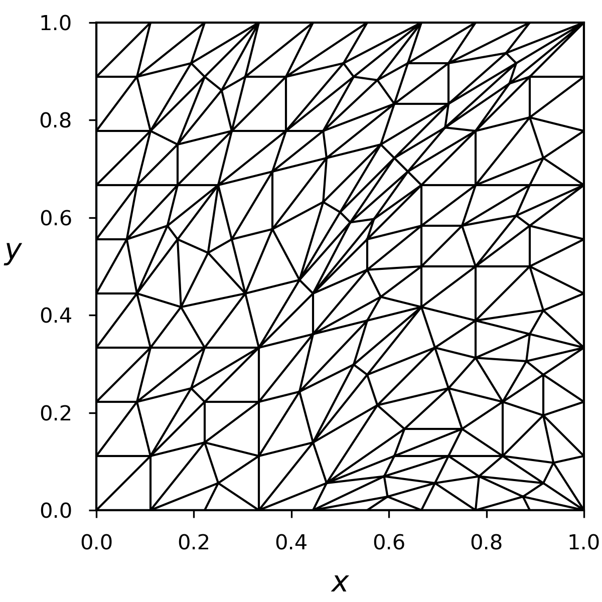
I divide the domain into a triangular mesh using the recursive kernel-based method described in Fernandez2017simultaneous. I consider four mesh levels; the level-2 mesh, which is the second coarsest mesh, is illustrated in Figure 6(a). In order to move from one level to the next, each element in the mesh is divided, in reference space, according to a canonical subdivision, i.e., the kernel mesh; for additional details, please see Fernandez2017simultaneous. My motivation for using this kernel-based set of meshes is to avoid meshes in which the element size varies smoothly from element to element. Such smooth meshes might unfairly bias the results in favor of the C-SBP discretization.

For a given mesh level, let denote the set of element subdomains:
Each triangle in is the image of the reference triangle, , under an appropriate mapping. For the linear-advection experiments, each triangle can be obtained from using an affine mapping; I will discuss curvilinear elements in the context of the Euler equations.
The D-SBP discretization is the same as the one described in Fernandez2017simultaneous and uses the and SBP- operators introduced in that same paper. The and operators from Fernandez2017simultaneous were not used in the present studies, since they have only exact cubatures. Instead, I created new and operators that have exact cubatures using the procedure described in Fernandez2017simultaneous. Consequently, both the D-SBP and C-SBP discretizations use operators based on exact cubatures.
Although the C-SBP discretization has been described throughout this paper, I need to clarify two details for this numerical experiment. First, based on the affine-mapping assumption, the global first-derivative SBP operators are given by
| where | |||
| (18) | |||
| (19) | |||
| and | |||
| (20) | |||
where is the determinant of the mapping Jacobian on element . The Jacobian terms — , , , and — and the determinant are constant over each element, so they can be computed either analytically or using the local SBP operators.
The second point that needs clarifying is the scaling function that appears in LPS. For dimensional consistency, I use the magnitude of the advection velocity in reference space:
where
Again, since the Jacobian is constant over each element, the scalar can either be computed analytically or using the SBP operators.
Finally, the C-SBP and D-SBP semi-discretizations are both advanced in time using the classical fourth-order Runge-Kutta method. I chose the time-step size for each discretization using the results of the eigenvalue spectra study, presented next.
5.1.1 Investigation of operator spectrum
The eigenvalues of the spatial operators are plotted in Figure 7. These spectra are from discretizations on the level 2 mesh shown in Figure 6(a).
I have scaled each set of eigenvalues by the corresponding spectral radius, so the axes can use the same scale. To indicate the relative size of the spectral-radius scaling, each figure includes the effective time step, , that the discretization would need to take relative to the C-SBP scheme. For example, if is the spectral radius of the C-SBP scheme, and is the spectral radius of the D-SBP scheme, than the effective time step is
For , , and the C-SBP discretizations have larger effective time steps. For the D-SBP scheme has a slightly larger time step of versus .
Qualitatively, the spectra of the C-SBP and D-SBP are quite distinct. As increases, the C-SBP spectra cluster closer and closer to the imaginary axis. In contrast, the D-SBP spectra remain clustered within a disk-shaped region. This suggests that the C-SBP discretization may approximate the infinite-dimensional spectrum, which is pure imaginary, more efficiently than the D-SBP discretization.


5.1.2 accuracy study
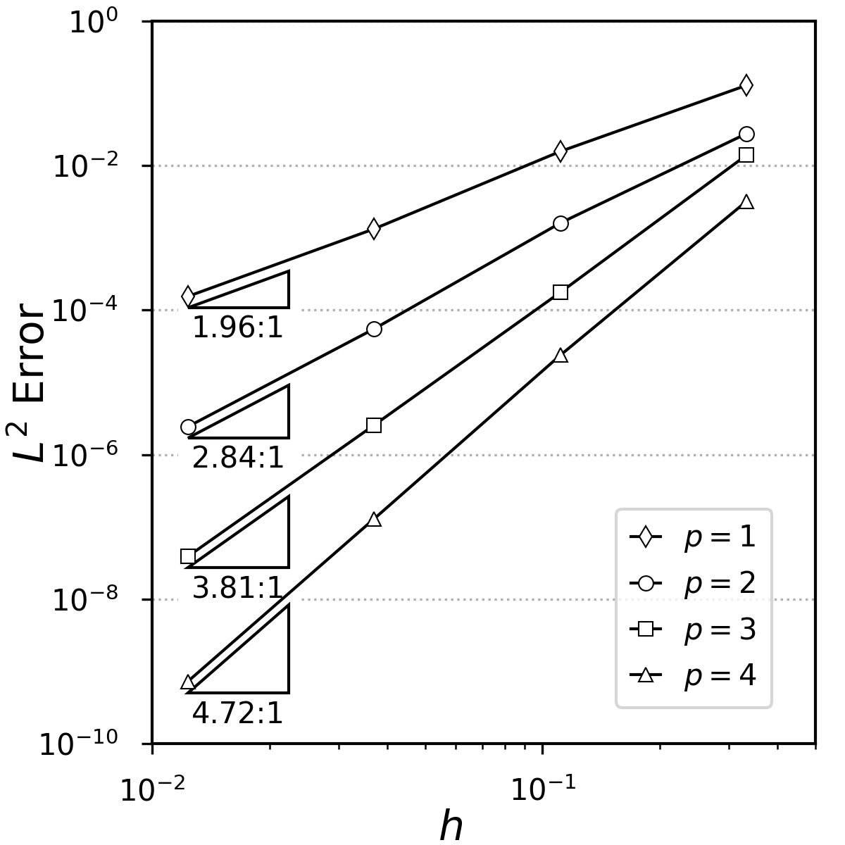
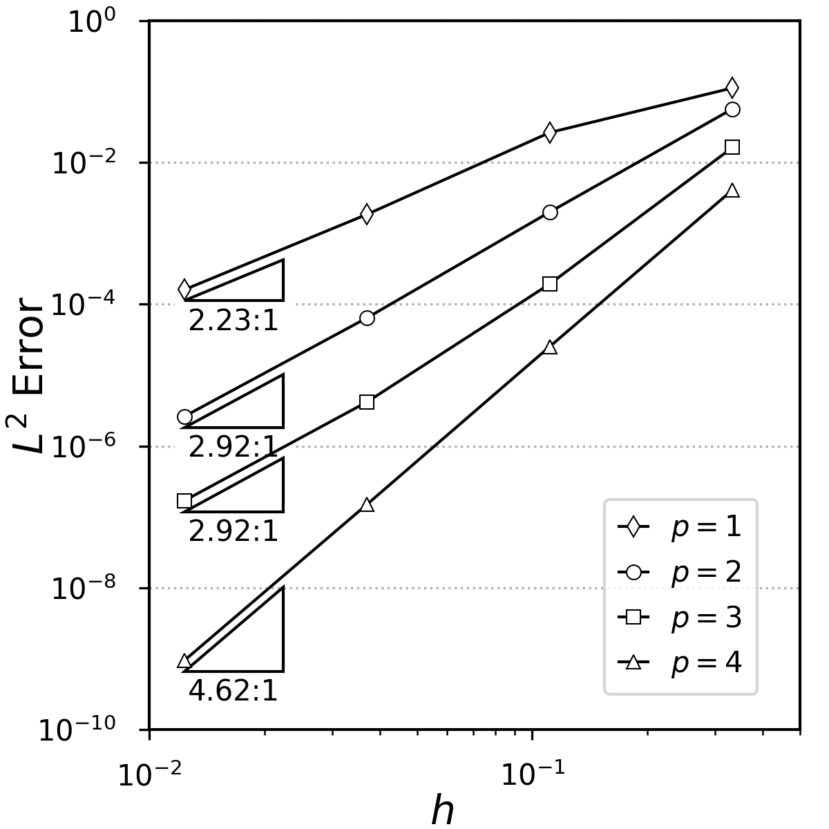
I used all four mesh levels to conduct a mesh convergence study for the linear-advection equation. The objective of this study was to verify that the C-SBP discretization achieves optimal, or near optimal, rates of convergence in the norm. Furthermore, I wanted to investigate the relative error between the C-SBP and D-SBP schemes on the same mesh.
The equations were marched forward in time using the classical fourth-order Runge-Kutta method. The spectra in the previous section were used to identify the maximum stable time step for each discretization. Although the spectra were gathered for only one mesh, I observed that the ratio between the reference spectral radius, , and the other spectral radii remained roughly constant across mesh levels. Thus, for a given mesh level and discretization, the maximum stable time step can be determined from the ratios in Figure 7 and the maximum reference time step for the C-SBP scheme. For example, if , then for the D-SBP scheme.
The spectral radius was not available for the C-SBP discretization on the finest mesh; therefore, in order to estimate the maximum reference time step, i.e. , I fit the following model for the spectral radius:
where lev is the mesh level, and is a nominal element size for the kernel-based mesh: each edge is split into thirds during refinement, hence the factor of . I used the spectral radii from the and meshes to fit the above model and found that and . The resulting fit predicts for the discretization on the level 1 mesh, which is a 6% error from the true spectral radius of .
I advanced the solution in time one period, to , which brings the bell-shaped solution back to its initial position. The error between the numerical solution at and the initial condition was then evaluated. I used the SBP norm matrices and Jacobian determinant to approximate the integrals in the norm of the error.
Figures 8(a) and Figures 8(b) plot the error versus the nominal element size for the C-SBP and D-SBP discretizations. For a given and mesh size, the errors for the two discretizations are comparable. The asymptotic convergence rates are estimated using the error on the finest two grid levels and are displayed beneath the rate triangles in Figure 8.
5.1.3 Efficiency study
To assess the relative efficiency of the C-SBP and D-SBP discretizations, I have plotted the solution error versus normalized CPU time in Figure 9. The times are normalized by the C-SBP discretization on the coarsest mesh. The Julia code that I wrote to gather these results used pre-allocated work arrays to avoid expensive memory allocation, and was run on Julia version 0.6.2 with array-bound checking turned off.
The results in Figure 9 indicate that the C-SBP discretizations are more efficient than the D-SBP discretizations up to polynomial degree , at which point the two schemes are comparable. Admittedly, this is only one simple test case, and it is likely that improvements could be made to both schemes. Furthermore, these results do not shed much light on the relative efficiency of the discretizations in the context of implicit time-marching schemes, viscous terms, and three-dimensional problems. Nevertheless, the results in Figure 9 suggest that, at the very least, C-SBP schemes warrant further investigation.

5.2 Euler equations
The remaining numerical experiments are used to assess the C-SBP entropy-stable discretization of the Euler equations described in Section 3. In particular, I am interested in verifying accuracy in the context of a nonlinear system of equations, as well as verifying entropy conservation and stability.
The following studies use curvilinear elements, in contrast to the affine elements adopted for the linear-advection studies. To ensure entropy conservation and stability, I evaluated the mapping Jacobian as described in Crean2018entropy. In fact, since I considered exclusively two-dimensional meshes, I used Lagrange elements to define the coordinate transformation and computed the metrics analytically. I then used equations (23)–(25) from Crean2018entropy to define the SBP operators on each element. The resulting operators satisfy the theoretical requirements for entropy conservation and stability, but they not satisfy the polynomial-exactness condition 1 in Definition 1; with the exception of constant functions, the operators differentiate polynomials only in an asymptotic sense as the mesh is refined. This motivates the accuracy study, which I discuss next.
5.2.1 Accuracy verification using the steady vortex
The steady isentropic vortex is an exact, smooth solution to the Euler equations, which makes it suitable for verifying the accuracy of the C-SBP entropy-stable discretization. The vortex flow has circular symmetry about the origin. Specifically, its streamlines are concentric circles and its density is given by
where denotes the radial polar coordinate; is a reference radius, and and are the density and Mach number at , respectively. The remaining conservative variables can be obtained using the isentropic relations.
The domain for the steady-vortex problem is the quarter annulus . I applied an inviscid “slip” boundary condition, , along the inner radius, . On the remaining boundaries, I provided the exact solution to characteristic-type boundary conditions. Both boundary conditions are implemented in a dual-consistent manner Lu2005posteriori; Hartmann2007adjoint; Hicken2014dual, which, as we shall see, is important for functional accuracy.
Remark 11
While the boundary conditions are dual consistent, they are not entropy stable. Entropy-stable boundary conditions have been proposed Svard2013entropy, but they are not needed for this steady problem.
I created the meshes for by uniformly dividing the domain into quadrilaterals in polar coordinates. Each quadrilateral was then subdivided into two triangles. For a degree SBP discretization, the coordinate mapping for each triangle was represented using a Lagrange basis with uniformly spaced nodes. The coordinate mapping was then uniquely determined by mapping the Lagrange nodes to physical space. The resulting curvilinear elements were used to define the locations of the SBP nodes (in physical space) and the mapping Jacobian according to Crean2018entropy.
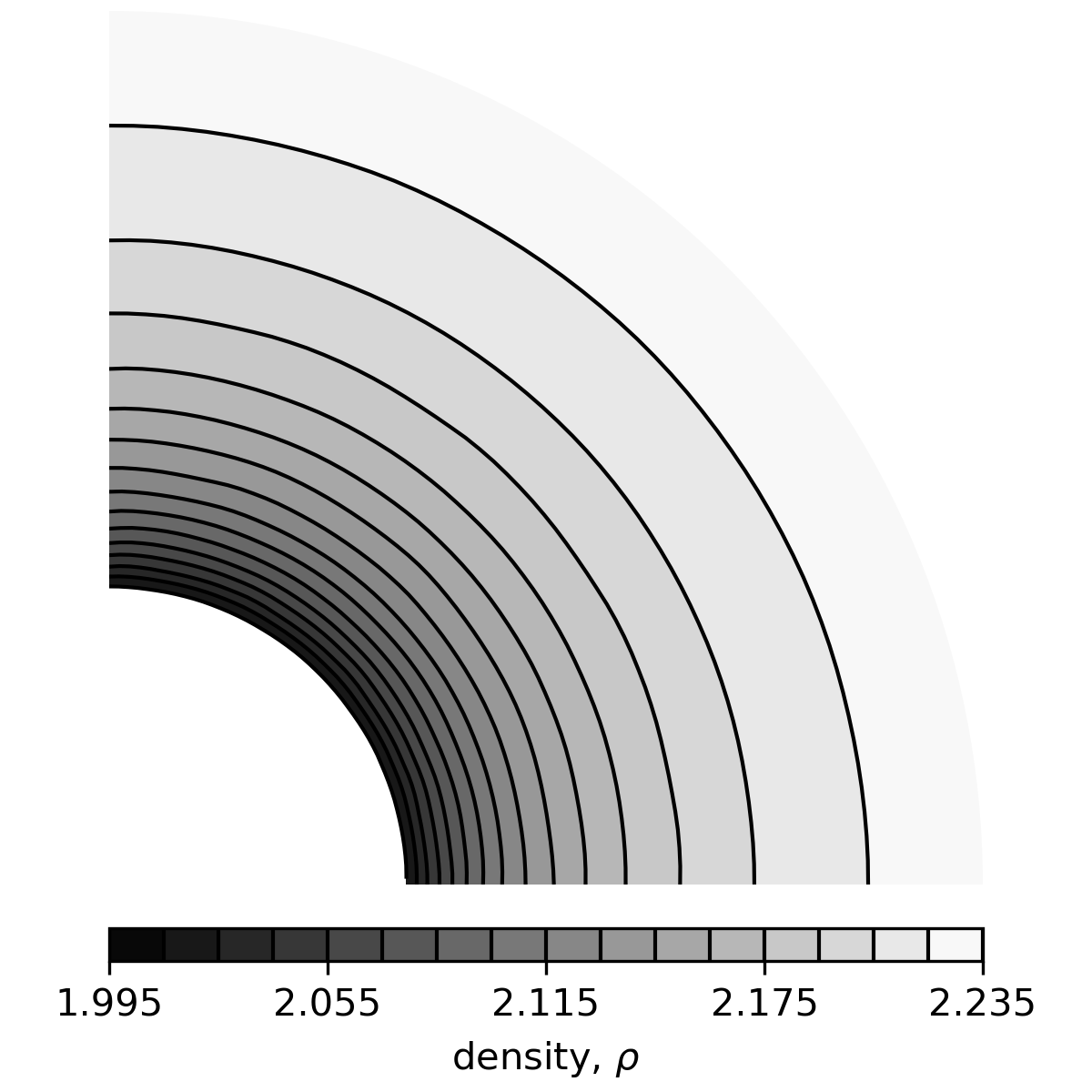
Figure 10(a) shows the mesh with edges along each boundary, and Figure 10(b) plots the discrete density of the corresponding C-SBP discretization. All steady-vortex solutions were obtained using Newton’s method combined with a sparse direct solver.

The density error is plotted versus the nominal mesh size, , in Figure 11(a). I estimated the asymptotic convergence rates, which are listed under the triangles in Figure 11(a), using the errors on the finest two grids. For this problem the C-SBP schemes have rates close to .
I conclude this accuracy study by assessing the drag force on the inner radius . Boundary functionals, such as drag, are important in many CFD applications, and a discretization is often judged based on how accurate it can estimate such outputs. Figure 11(b) plots the drag error versus mesh size for the C-SBP discretizations. For all polynomial degrees under consideration, we see that the drag is superconvergent. For the and discretizations, the rate is approximately . The asymptotic rate is less clear for the two higher-order schemes, because the drag values on the finest grid(s) are impacted by round-off errors.


5.2.2 Entropy-conservation and -stability verification
For the final set of results, I solved the discretized Euler equations on a periodic domain with a discontinuous initial condition. The objective was to verify the entropy-conservation and entropy-stability properties of the C-SBP discretization on a non-trivial flow. I did not consider accuracy, nor did I consider “monotonicity” preservation; these remain important issues in the context of discontinuous flows and will constitute future work.
The domain was the unit square, , with periodic boundary conditions. The mesh generation process began by creating a uniform quadrilateral mesh in a reference space, . Next, each quad was subdivided into a triangle. As with the steady vortex case, the coordinate transformation was defined by assigning a Lagrange element to each triangle, and then mapping the Lagrange nodes to physical space based on the transformation
Figure 12(a) illustrates the mesh. The meshes for the other degrees had similar shaped elements, but they obviously had more nodes per element.
The initial condition was similar to the one used in Fernandez2018staggered and was defined by
The analytical initial condition is shown in Figure 12(b). I advanced the solution in time from to non-dimensional units using the implicit midpoint rule, rather than the RK4 scheme adopted for the linear-advection study. I found that, despite its slower rate of convergence, the midpoint rule produced a smaller entropy-conservation error for the problem and time steps that were considered.


The set of plots in Figure 13 show the change in total entropy versus time for the entropy-conservative discretization (11); there is one plot for each degree under consideration. If denotes the nodal values of the (mathematical) entropy at time step , then the change in entropy is defined by
Most time discretizations are not entropy conservative, so will be non-zero even though the semi-discrete scheme (11) is entropy conservative. This is reflected in Figure 13, which shows that the change in entropy is indeed non-zero. To verify that this entropy-conservation error is due to the temporal discretization, I ran the simulations using a CFL of 0.1 and 0.01. With this change in time step size, one would expect the entropy-conservation error to decrease by two orders of magnitude, since the implicit midpoint rule is second-order accuracy. This is confirmed by the results in Figure 13; the magnitude in the entropy fluctuations is reduced by two orders of magnitude between CFL=0.1 and CFL=0.01, as expected.


When the entropy-stable LPS terms are included, Theorem 3.2 tells us that the change in entropy should always be negative. Again, this is only guaranteed for the semi-discrete scheme, so it is possible that a particular time discretization may lead to entropy growth. However, this is not the case for the present simulations using the implicit midpoint rule, as Figure 14 demonstrates. This figure plots the change in entropy from one time step to the next, and it shows that this change is always negative, so entropy is non-increasing.

6 Summary and Discussion
Summation-by-parts (SBP) operators have received renewed interest in recent years, because they can be used to implement entropy-stable, high-order CFD methods. The focus of this renewed interest has been discontinuous-Galerkin-type discretizations, and limited, if any, attention has been paid to continuous-Galerkin analogies, despite their efficiency for low to moderate orders of accuracy. To address this gap, I have presented a high-order, entropy-stable C-SBP discretization that uses a continuous representation of the solution.
The baseline C-SBP discretization is neutrally stable, so an important goal of this work was to develop a stabilization that is simultaneously entropy stable, well conditioned, and element local. To meet these requirements, I advocated the use of additional nodal degrees of freedom to enable local-projection stabilization (LPS) at the element level. While this solution is not optimal from the perspective of approximation theory, it is well suited to diagonal-norm SBP operators, which typically require more nodes than necessary for a degree polynomial basis.
For completeness, I reviewed the construction of the SBP operators used in this work. The operators, which are designed for triangular elements, have exact norms, vertex nodes, and diagonal boundary operators. I also described three methods of constructing LPS operators; one suitable for degree exact cubatures, one suitable for exact cubatures, and one suitable for finite-difference discretizations more generally.
I verified the C-SBP discretizations using the linear advection equation and the Euler equations. The discretizations exhibited near optimal, rates of convergence, as well as superconvergent functionals when implemented in a dual-consistent manner. The results also established that the baseline C-SBP discretization is entropy conservative, and that LPS is entropy stable when applied to the entropy variables directly.
The results suggest that C-SBP discretizations are competitive with D-SBP discretizations for moderate degree discretizations, where the interface penalties in D-SBP methods represent a significant fraction of the total computational expense. Thus, I suspect that the C-SBP discretization will be most attractive when the discretization error is dominated by errors in some phenomenological model(s), such as a turbulence closure. At the very least, the continuous approach warrants a closer examination than it has in the past.
7 Acknowledgments
My sincerest thanks to my students — Anthony Ashley, Tucker Babcock, Garo Bedonian, Luiz Cagliari, Jared Crean, Sharanjeet Kaur, Kinshuk Panda, Ge Yan, and Jianfeng Yan — for their feedback on an early draft of this paper.
All the results in this paper were obtained using software written in Julia Bezanson2017julia. The plots were generated using Matplotlib Hunter2007matplotlib, with help from the Numpy Oliphant2006guide; Van2011numpy and Scipy Jones2001Scipy libraries.
References
- (1) Baiocchi, C., Brezzi, F., Franca, L.P.: Virtual bubbles and Galerkin-least-squares type methods (Ga.L.S.). Computer Methods in Applied Mechanics and Engineering 105(1), 125–141 (1993). DOI 10.1016/0045-7825(93)90119-i. URL http://dx.doi.org/10.1016/0045-7825(93)90119-i
- (2) Barth, T.J.: Numerical methods for gasdynamic systems on unstructured meshes. In: An introduction to recent developments in theory and numerics for conservation laws, pp. 195–285. Springer (1999)
- (3) Becker, R., Braack, M.: A finite element pressure gradient stabilization for the stokes equations based on local projections. Calcolo 38(4), 173–199 (2001). DOI 10.1007/s10092-001-8180-4. URL http://dx.doi.org/10.1007/s10092-001-8180-4
- (4) Bezanson, J., Edelman, A., Karpinski, S., Shah, V.B.: Julia: A fresh approach to numerical computing. SIAM review 59(1), 65–98 (2017)
- (5) Braack, M., Lube, G.: Finite elements with local projection stabilization for incompressible flow problems. Journal of Computational Mathematics (2/3), 116–147 (2009)
- (6) Brooks, A.N., Hughes, T.J.R.: Streamline upwind/Petrov-Galerkin formulations for convection dominated flows with particular emphasis on the incompressible Navier-Stokes equations. Computer Methods in Applied Mechanics and Engineering 32(1-3), 199–259 (1982). DOI 10.1016/0045-7825(82)90071-8
- (7) Burman, E., Fernández, M.A., Hansbo, P.: Continuous Interior Penalty Finite Element Method for Oseen’s Equations. SIAM Journal on Numerical Analysis 44(3), 1248–1274 (2006). DOI 10.1137/040617686. URL http://dx.doi.org/10.1137/040617686
- (8) Burman, E., Hansbo, P.: Edge stabilization for galerkin approximations of convection–diffusion–reaction problems. Computer Methods in Applied Mechanics and Engineering 193(15-16), 1437–1453 (2004). DOI 10.1016/j.cma.2003.12.032. URL http://dx.doi.org/10.1016/j.cma.2003.12.032
- (9) Carpenter, M.H., Fisher, T.C., Nielsen, E.J., Frankel, S.H.: Entropy stable spectral collocation schemes for the Navier–Stokes equations: Discontinuous interfaces. SIAM Journal on Scientific Computing 36(5), B835–B867 (2014). DOI 10.1137/130932193. URL http://dx.doi.org/10.1137/130932193
- (10) Chandrashekar, P.: Kinetic energy preserving and entropy stable finite volume schemes for compressible euler and Navier-Stokes equations. Communications in Computational Physics 14(5), 1252–1286 (2015). DOI 10.4208/cicp.170712.010313a. URL http://dx.doi.org/10.4208/cicp.170712.010313a
- (11) Chen, T., Shu, C.W.: Entropy stable high order discontinuous Galerkin methods with suitable quadrature rules for hyperbolic conservation laws. Journal of Computational Physics 345, 427–461 (2017). DOI 10.1016/j.jcp.2017.05.025. URL http://dx.doi.org/10.1016/j.jcp.2017.05.025
- (12) Cockburn, B., Hou, S., Shu, C.W.: The Runge-Kutta local projection discontinuous galerkin finite element method for conservation laws. IV: The multidimensional case. Mathematics of Computation 54(190), 545+ (1990). DOI 10.2307/2008501. URL http://dx.doi.org/10.2307/2008501
- (13) Cools, R.: Monomial cubature rules since “stroud”: a compilation — part 2. Journal of Computational and Applied Mathematics 112(1–2), 21 – 27 (1999). DOI http://dx.doi.org/10.1016/S0377-0427(99)00229-0. URL http://www.sciencedirect.com/science/article/pii/S0377042799002290
- (14) Craig Penner, D., Zingg, D.W.: High-Order artificial dissipation operators possessing the Summation-By-parts property. In: 2018 Fluid Dynamics Conference. American Institute of Aeronautics and Astronautics (2018). DOI 10.2514/6.2018-4165. URL http://dx.doi.org/10.2514/6.2018-4165
- (15) Crean, J., Hicken, J.E., Del Rey Fernández, D.C., Zingg, D.W., Carpenter, M.H.: Entropy-stable summation-by-parts discretization of the Euler equations on general curved elements. Journal of Computational Physics 356, 410–438 (2018). DOI 10.1016/j.jcp.2017.12.015
- (16) Crean, J., Panda, K., Ashley, A., Hicken, J.E.: Investigation of stabilization methods for multi-dimensional summation-by-parts discretizations of the Euler equations. In: 54th AIAA Aerospace Sciences Meeting, p. 13. San Diego, California, United States (2016). DOI 10.2514/6.2016-1328. URL https://dl.dropboxusercontent.com/u/38627164/Website/papers/Crean_etal_stab_methods_SBP_AIAA-2016-1328.pdf. AIAA 2016-1328
- (17) Dafermos, C.M.: Hyperbolic Conservation Laws in Continuum Physics, vol. 325. Springer Berlin Heidelberg, Berlin, Heidelberg (2010). DOI 10.1007/978-3-642-04048-1. URL http://dx.doi.org/10.1007/978-3-642-04048-1
- (18) Del Rey Fernández, D.C., Boom, P.D., Zingg, D.W.: A generalized framework for nodal first derivative summation-by-parts operators. Journal of Computational Physics 266(1), 214–239 (2014)
- (19) Del Rey Fernández, D.C., Boom, P.D., Zingg, D.W.: A generalized framework for nodal first derivative summation-by-parts operators. Journal of Computational Physics 266(1), 214–239 (2014)
- (20) Del Rey Fernández, D.C., Crean, J., Carpenter, M.H., Hicken, J.E.: Staggered-grid entropy-stable multidimensional summation-by-parts discretizations on curvilinear coordinates. (Submitted to the Journal of Scientific Computing) (2018)
- (21) Del Rey Fernández, D.C., Hicken, J.E., Zingg, D.W.: Review of summation-by-parts operators with simultaneous approximation terms for the numerical solution of partial differential equations. Computers & Fluids 95(22), 171–196 (2014)
- (22) Del Rey Fernández, D.C., Hicken, J.E., Zingg, D.W.: Simultaneous Approximation Terms for Multi-dimensional Summation-by-Parts Operators. Journal of Scientific Computing pp. 1–28 (2017). DOI 10.1007/s10915-017-0523-7
- (23) Douglas, J., Dupont, T.: Interior Penalty Procedures for Elliptic and Parabolic Galerkin Methods Computing Methods in Applied Sciences. In: R. Glowinski, J.L. Lions (eds.) Computing Methods in Applied Sciences, Lecture Notes in Physics, vol. 58, chap. 6, pp. 207–216. Springer Berlin / Heidelberg, Berlin, Heidelberg (1976). DOI 10.1007/bfb0120591. URL http://dx.doi.org/10.1007/bfb0120591
- (24) Fisher, T.C.: High-order l2 stable multi-domain finite difference method for compressible flows. Ph.D. thesis, Purdue University (2012)
- (25) Fisher, T.C., Carpenter, M.H.: High-order entropy stable finite difference schemes for nonlinear conservation laws: Finite domains. Journal of Computational Physics 252, 518–557 (2013). DOI 10.1016/j.jcp.2013.06.014. URL http://dx.doi.org/10.1016/j.jcp.2013.06.014
- (26) Fisher, T.C., Carpenter, M.H., Nordström, J., Yamaleev, N.K., Swanson, C.: Discretely conservative finite-difference formulations for nonlinear conservation laws in split form: Theory and boundary conditions. Journal of Computational Physics 234, 353–375 (2013). DOI 10.1016/j.jcp.2012.09.026. URL http://dx.doi.org/10.1016/j.jcp.2012.09.026
- (27) Gassner, G.J.: A Skew-Symmetric discontinuous galerkin spectral element discretization and its relation to SBP-SAT finite difference methods. SIAM Journal on Scientific Computing 35(3), A1233–A1253 (2013). DOI 10.1137/120890144. URL http://dx.doi.org/10.1137/120890144
- (28) Gassner, G.J.: A skew-symmetric discontinuous Galerkin spectral element discretization and its relation to SBP-SAT finite difference methods. SIAM Journal on Scientific Computing 35(3), A1233–A1253 (2013)
- (29) Hartmann, R.: Adjoint consistency analysis of discontinuous Galerkin discretizations. SIAM Journal on Numerical Analysis 45(6), 2671–2696 (2007). DOI 10.1137/060665117. URL http://dx.doi.org/10.1137/060665117
- (30) Hesthaven, J.S., Warburton, T.: Nodal discontinuous Galerkin methods: algorithms, analysis, and applications. Springer-Verlag, New York (2008)
- (31) Hicken, J.E., Del Rey Fernández, D.C., Zingg, D.W.: Multi-dimensional summation-by-parts operators: General theory and application to simplex elements. SIAM Journal on Scientific Computing 38(4), A1935–A1958 (2016)
- (32) Hicken, J.E., Zingg, D.W.: Summation-by-parts operators and high-order quadrature. Journal of Computational and Applied Mathematics 237(1), 111–125 (2013). DOI 10.1016/j.cam.2012.07.015. URL http://dx.doi.org/10.1016/j.cam.2012.07.015
- (33) Hicken, J.E., Zingg, D.W.: Dual consistency and functional accuracy: a finite-difference perspective. Journal of Computational Physics 256, 161–182 (2014). DOI 10.1016/j.jcp.2013.08.014. URL http://dx.doi.org/10.1016/j.jcp.2013.08.014
- (34) Hughes, T.J.R.: Multiscale phenomena: Green’s functions, the Dirichlet-to-Neumann formulation, subgrid scale models, bubbles and the origins of stabilized methods. Computer Methods in Applied Mechanics and Engineering 127, 387–401 (1995). DOI 10.1016/0045-7825(95)00844-9. URL http://dx.doi.org/10.1016/0045-7825(95)00844-9
- (35) Hughes, T.J.R., Franca, L.P., Hulbert, G.M.: A new finite element formulation for computational fluid dynamics: VIII. The galerkin/least-squares method for advective-diffusive equations. Computer Methods in Applied Mechanics and Engineering 73(2), 173–189 (1989). DOI 10.1016/0045-7825(89)90111-4. URL http://dx.doi.org/10.1016/0045-7825(89)90111-4
- (36) Hughes, T.J.R., Franca, L.P., Mallet, M.: A new finite element formulation for computational fluid dynamics: I. symmetric forms of the compressible Navier-Stokes equations and the second law of thermodymaics. Computer Methods in Applie Mechanics and Engineering 54(2), 223–234 (1986)
- (37) Hunter, J.D.: Matplotlib: A 2d graphics environment. Computing In Science & Engineering 9(3), 90–95 (2007). DOI 10.1109/MCSE.2007.55
- (38) Ismail, F., Roe, P.L.: Affordable, entropy-consistent euler flux functions II: Entropy production at shocks. Journal of Computational Physics 228(15), 5410–5436 (2009). DOI 10.1016/j.jcp.2009.04.021. URL http://dx.doi.org/10.1016/j.jcp.2009.04.021
- (39) Jameson, A., Schmidt, W., Turkel, E.: Numerical solution of the Euler equations by finite volume methods using Runge-Kutta time-stepping schemes. In: 14th Fluid and Plasma Dynamics Conference. Palo Alto, CA (1981)
- (40) Jones, E., Oliphant, T., Peterson, P., et al.: SciPy: Open source scientific tools for Python (2001–). URL http://www.scipy.org/. [Online; accessed ¡today¿]
- (41) Liu, Y., Vinokur, M.: Exact integrations of polynomials and symmetric quadrature formulas over arbitrary polyhedral grids. Journal of Computational Physics 140(1), 122–147 (1998). DOI http://dx.doi.org/10.1006/jcph.1998.5884. URL http://www.sciencedirect.com/science/article/pii/S0021999198958843
- (42) Lu, J.C.: An a posteriori error control framework for adaptive precision optimization using discontinuous Galerkin finite element method. Ph.D. thesis, Massachusetts Institute of Technology, Cambridge, Massachusetts (2005)
- (43) Mattsson, K., Svärd, M., Nordström, J.: Stable and accurate artificial dissipation. Journal of Scientific Computing 21(1), 57–79 (2004)
- (44) Oliphant, T.E.: A guide to NumPy, vol. 1. Trelgol Publishing USA (2006)
- (45) Parsani, M., Carpenter, M.H., Fisher, T.C., Nielsen, E.J.: Entropy Stable Staggered Grid Discontinuous Spectral Collocation Methods of any Order for the Compressible Navier–Stokes Equations. SIAM Journal on Scientific Computing 38(5), A3129–A3162 (2016). DOI 10.1137/15m1043510. URL http://dx.doi.org/10.1137/15m1043510
- (46) Pulliam, T.H.: Artificial dissipation models for the euler equations. AIAA Journal 24(12), 1931–1940 (1986)
- (47) Ranocha, H., Glaubitz, J., Öffner, P., Sonar, T.: Stability of artificial dissipation and modal filtering for flux reconstruction schemes using summation-by-parts operators. Applied Numerical Mathematics 128, 1–23 (2018). DOI 10.1016/j.apnum.2018.01.019. URL http://dx.doi.org/10.1016/j.apnum.2018.01.019
- (48) Svärd, M., Nordström, J.: Review of summation-by-parts schemes for initial-boundary-value-problems. Journal of Computational Physics 268(1), 17–38 (2014)
- (49) Svärd, M., Özcan, H.: Entropy-Stable Schemes for the Euler Equations with Far-Field and Wall Boundary Conditions. Journal of Scientific Computing 58(1), 61–89 (2013). DOI 10.1007/s10915-013-9727-7. URL http://dx.doi.org/10.1007/s10915-013-9727-7
- (50) Tadmor, E.: The numerical viscosity of entropy stable schemes for systems of conservation laws i. Mathematics of Computation 49(179), 91–103 (1987)
- (51) Tadmor, E.: Entropy stability theory for difference approximations of nonlinear conservation laws and related time-dependent problems. Acta Numerica 12, 451–512 (2003). DOI 10.1017/s0962492902000156. URL http://dx.doi.org/10.1017/s0962492902000156
- (52) Van Der Walt, S., Colbert, S.C., Varoquaux, G.: The numpy array: a structure for efficient numerical computation. Computing in Science & Engineering 13(2), 22 (2011)