Chemistry Along Accretion Streams in a Viscously-Evolving Protoplanetary DiskRADMC-3D (Dullemond et al. 2012), Computation of isochrones (Siess et al. 2000)
Abstract
The composition of a protoplanetary disk is set by a combination of interstellar inheritance and gas and grain surface chemical reactions within the disk. The survival of inherited molecules, as well as the disk in situ chemistry depends on the local temperature, density and irradiation environment, which can change over time due to stellar and disk evolution, as well as transport in the disk. We address one aspect of this coupling between the physical and chemical evolution in disks by following accretion streamlines of gas and small grains in the disk midplane, while simultaneously taking the evolving star into account. This approach is computationally efficient and enables us to take into account changing physical conditions without reducing the chemical network. We find that many species are enhanced in the inner disk midplane in the dynamic model due to inward transport of cosmic-ray driven chemical products, resulting in, e.g., orders-of magnitude hydrocarbon enhancements at 1 au, compared to a static disk. For several other chemical families, there is no difference between the static and dynamic models, indicative of a robust chemical reset, while yet others show differences between static and dynamic models that depend on complex interactions between physics and chemistry during the inward track. The importance of coupling dynamics and chemistry when modeling the chemical evolution of protoplanetary disks is thus depends on what chemistry is of interest.
Keywords:
accretion disks; protoplanetary disksI Introduction
Planets form in the dust- and gas-rich disks around young stars, i.e., in protoplanetary disks. The chemical composition of the disk directly impacts the compositions of forming planets and planetesimals. Rocky planets, ice giants, and comets all assemble mainly from disk solids, and their composition depends on the refractory and volatile content of dust grains. By contrast, gas giants obtain much of their mass directly from the disk gas, and their composition therefore depends on both the disk’s gas and dust chemical compositions (Mizuno 1980; Bodenheimer & Pollack 1986; Öberg et al. 2011; Kokubo & Ida 2012; Cridland et al. 2016; Cridland et al. 2017b, e.g.,).
The chemistry of the disk spatially varies due to gradients in radiation fields, temperature and density structures, and cosmic ray attenuation. These effects act to produce a radially-changing disk molecular composition (Aikawa et al. 1997; Willacy & Langer 2000; Bergin et al. 2007, e.g.,). Moreover, at the relevant pressures and densities, much of the disk does not reach local steady state within the few million year lifetime of the gas disk (Aikawa et al. 1998, e.g.,). Chemical processing of the material can thus have a significant effect on the planetesimals’ compositions (Eistrup et al. 2016). Accurately predicting the time-evolving chemical history of a disk and comparing with observations of disk gas are therefore key to understanding what compositions planets can potentially acquire.
Observations of molecules in disks are limited (McGuire 2018) due to their low masses, relatively cool temperatures, and small angular extents. The inner disk () is observed to have gas-phase molecules like , CO, nitrogen-bearing species, and hydrocarbons. Spitzer observations of the upper disk layers in the inner disk suggest a partial “reset-like” chemistry (Pontoppidan et al. 2014) due to the extreme densities, temperatures, and radiation fields close to the star. As shown in this study, this chemistry is expected to be modified by continuous inward transport of molecules formed in the outer parts of the disk, resulting in deviations from steady-state chemistry.
The outer disk (), on the other hand, is characterized by sequential freeze-out of abundant volatiles (Henning & Semenov 2013) and a slower chemical conversion that may preserve more of the disk’s initial composition, as set by the molecular cloud. In this region, the relative importance of inheritance and in situ chemical processing depends on the vertical location within the disk. For ice in the midplane, models demonstrate that the outer disk likely exhibits an “inheritance-like” chemistry, where the timescales for chemical evolution can be longer than the disk lifetime, thus processing little of the ice (Semenov & Wiebe 2011; Cleeves et al. 2014b). For cyanide species, observations are more consistent with chemical reprocessing (Öberg et al. 2015).
These different results can, in part, be explained by strong vertical gradients in physical conditions in the outer disk. The uppermost, surface layer experiences strong irradiation, so relatively fast photochemistry dominates. Beneath the surface layer is a warm molecular layer where ion–molecule chemistry chemistry dominates; CO is present but is frozen out onto grains. Finally, close to the midplane, molecules freeze out onto grains and slow grain surface reactions dominate the chemistry (Henning & Semenov 2013).
Modeling disk chemistry is complicated by the fact that disks and their host stars are dynamic — densities, temperatures and radiation fields all evolve with time. Theory and observations show that protoplanetary disks are actively accreting (Lynden-Bell & Pringle 1974; Gullbring et al. 1998, e.g.,), with some material transferred onto the star and some material moved outward, conserving angular momentum. Other dynamical processes that may be relevant include vertical mixing, turbulence, and grain drift and settling (Whipple 1973; Weidenschilling 1977; Morfill 1983; Weidenschilling & Cuzzi 1993; Hanner 1999; Bockelée-Morvan et al. 2002; Willacy et al. 2006; Semenov et al. 2006; Cridland et al. 2017a; Bacciotti et al. 2018). In addition to material physically moving in the disk, the star itself introduces an added complication since it, too, is evolving in time (Siess et al. 1997, e.g.,), changing the incident radiation field and temperature profile of the disk.
The most common astrochemical treatment of a viscously-evolving disk is to fix the physical conditions to their local values at a given time and allow the chemistry to evolve at these fixed conditions. A handful of models have explored the coupling of some dynamical processes and chemistry. Early examples of coupling chemistry with accretion flows include Bauer et al. 1997 (and subsequent papers) and Aikawa et al. 1999. Nomura et al. 2009 followed the chemistry along simple streamlines in an -disk model and assumed a constant accretion rate. Heinzeller et al. 2011 used the same physical model with the addition of X-ray heating and investigated the effects of radial accretion, turbulent mixing, and disk winds. Including accretion in the model caused significant changes in the chemical composition of the disk midplane. Cridland et al. 2016 and Cridland et al. 2017b used the Chambers 2009 analytic model of viscous disk accretion to investigate the relationship between disk chemistry and planetary atmospheres, finding that the location and time at which the planet atmosphere accretes its atmosphere strongly affects its composition.
We build on these previous efforts and follow local physical conditions in accretion streams of gas and small, presumably coupled, grains in the disk midplane. We choose to focus on the midplane in this work because the gas and ice mantles on grains in the midplane eventually become available for incorporation into forming planetesimals, and because it allows some simplifying assumptions to be made regarding radiation fields and accretion stream geometries. This paper is structured as follows. In Section II, we introduce the method we use to trace both chemistry and physical conditions as functions of time. In Section III, we present the results of our model. We discuss and conclude our analysis in Sections IV and V, respectively.
II Methods
Our goal is to compute the time-dependent tracks that gas follows through a vicously evolving disk around an evolving pre-main sequence star and to solve for the chemical abundances along these tracks. Note that the tracks are treated as completely independent from one another, i.e., are not mixed, greatly simplifying the computation. Additionally, we treat the dust as well-coupled to the gas and do not address dust grain evolution, which may be chemically important. The main role of the dust is to provide surface area for chemical reactions. Dust growth and fragmentation fundamentally change the surface area to volume ratio of dust, however the dynamical evolution is more complex than can be treated in the present prescription, which we will address in future work.
One of the primary challenges to overcome in this method is that the surface density evolution and temperature structure are interdependent. To solve for both self-consistently, we use an iterative procedure, outlined in Figure 1.
II.1 Accretion disk model
We construct the physical disk model using the -disk framework (Shakura & Sunyaev 1973). We work in a cylindrical coordinate system parametrized by ; here, is the radial coordinate (distance from the star in the - plane), is the azimuthal angle, and is the vertical coordinate (height above the midplane).
The viscosity of an -disk is given by
| (1) |
where is the Keplerian angular velocity, is the local sound speed, is the local disk scale height determined by the midplane temperature, and is the stellar mass; we assume that the disk mass is negligible compared to . is a small dimensionless parameter with typical values to ; this range is supported observationally by, e.g., Flaherty et al. 2018, which found for the TW Hya disk. The sound speed is given by
| (2) |
where is the mean molecular weight of the gas, is the Boltzmann constant, and is the temperature of the gas and dust; we take the gas temperature equal to the dust temperature, which is reasonable in the disk midplane where the dust and gas are well-coupled through collisions (Henning & Semenov 2013). This temperature is computed and subsequently parametrized as a function of time and radius (see Section II.2).
We begin with the general surface density evolution equation (Pringle 1981; Clarke & Carswell 2007; Armitage 2010, e.g.,),
| (3) |
This equation can be derived from the Navier-Stokes and mass continuity equations for a fluid, as shown in Clarke & Carswell 2007. Because of the flexible form of the temperature we choose (see Section II.2), there exists no easily-found analytic solution for the surface density. Thus, we solve the equation numerically, using a simple finite difference scheme with second-order accurate spatial derivatives and a Crank-Nicoloson timestepping scheme. We implement this method using PETSc (Balay et al. 2018; Balay et al. 1997; Abhyankar et al. 2014).
Our initial surface density profile is informed by observations of disks, so we choose a form similar to
| (4) |
in the notation of, e.g., Andrews et al. 2012. However, for , a reasonable value based on observational fitting, this initial condition would approach infinity as approaches zero. This presents a computational challenge, because the value of cannot simply be fixed to a value at small radii due to disk evolution, yet an infinite value at is both unphysical and difficult to handle numerically. We circumvent this problem by introducing a sharp exponential taper at finite radius, given by
| (5) |
with shape parameters , , and that may be chosen freely. This function decays faster than Equation 4 blows up11 1 At first glance, it may appear that imposing zero surface density at finite radius inhibits accretion. However, if we examine the functional form of the accretion rate, (Pringle 1981), we see from Equation 10, which gives , that the factors of cancel; so the accretion rate can still be finite when approaches zero., so it is effective in producing the desired Dirichlet boundary condition22 2 A boundary condition in which the value of the unknown function is fixed to a given value at the boundaries only; in this case, the value zero is enforced. at small . Because Equation 4 decays exponentially at large , we do not need to introduce additional factors to produce a Dirichlet boundary condition at . In practice, then, we multiply Equation 4 by Equation 5 and then normalize to a chosen value , where is a chosen normalization radius. Parameters relevant to this model are listed in Table 1.
| Parameter | Symbol | Value |
|---|---|---|
| Stellar mass | ||
| Viscosity parameter | ||
| Mean molecular weight | ||
| Normalization radius | ||
| Shape parameter | ||
| normalization radius | ||
| Shape parameter | ||
| Shape parameter | ||
| Value of at | ||
| Exponential taper exponent | 4 | |
| Gas-to-dust ratio | ||
| Cosmic ray rate |
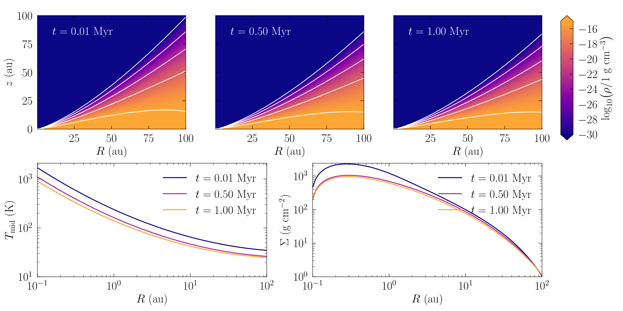
II.2 Disk temperature and density structures
As mentioned previously, we must assume a temperature structure to solve for the surface density, ultimately resulting in a new temperature structure. We use the Siess et al. 2000 isochrons for a , star to obtain the stellar radius and effective temperature on a linearly-spaced grid of given ages. We combine the dust density, assuming azimuthal symmetry, with the stellar parameters and compute the resulting dust temperature structure using RADMC-3D (Dullemond et al. 2012); at the end of the Monte Carlo simulation, the effects of accretion heating are added in flux space, so
| (6) |
and
| (7) |
(Hartmann 2009, e.g.). We iterate this procedure, fitting each time for the unknown parameters in our temperature model until the solutions converge to a relative precision of .
We assume a temperature function — which enters into Equation 3 through the viscosity term — that takes the flexible form
| (8) |
where is a dimensionless radius; ; and , , , , , and are parameters to be determined. We find that this large number of parameters is necessary to capture, with reasonable accuracy, the full radial- and time-dependent behavior of the disk temperature structure. The approximate final parameters we derive for this model are listed in Table 2. We do not use the raw temperatures from RADMC-3D because derivatives of the temperature function are needed for the time evolution of the surface density, and using the output without fitting would introduce unnecessary noise.
| Symbol | Value | Symbol | Value |
|---|---|---|---|
| K | 0.044 | ||
| 2.5 | -0.71 | ||
| 1.2 | 0.063 |
Once the temperature structure is known, the disk structure is fully determined at all times and radii. This information allows us to compute, for example, the disk mass and accretion rate as functions of time. These quantities are shown in Figure 3, from which we confirm that the accretion rate is reasonable.
We solve Equation 3 for a given set of temperature parameters to obtain the surface density at all radii and all times. We interpolate this function and obtain the gas density by assuming that it has a vertical Gaussian profile, i.e.
| (9) |
Further we adopt a gas-to-dust mass ratio of 100 at all radii, and assume only small micron-sized grains as prescribed in Fogel et al. 2011, such that the dust grains are well-coupled to the gas motion; we do not include larger grains here.
II.3 Computing tracks
For the physical model and stellar evolution described in the previous sections, we can compute self-consistent tracks of material through the disk following the velocity field implied by the evolving surface density profile. These tracks are given by the solution to the differential equation
| (10) |
(Clarke & Carswell 2007, e.g.,), where is the velocity in the radial direction. Once the solution for is known, this equation may be solved numerically. In Figure 4 we show several representative solutions with the temperature, density, surface density, and cosmic ray rate evaluated along the midplane tracks. Note that for many of the tracks the changes in temperature, density, and cosmic ray ionization are small to moderate. The only track that experiences order of magnitude changes in any of these physical variables is the 51 au track.
We follow tracks in the disk midplane for , the typical lifetime of a protoplanetary disk (Furlan et al. 2009; Mamajek 2009), with the exception of tracks that cross 1 au, in which case we stop the track as it is crossing. We impose the radius restriction to avoid any effects from our inner boundary condition, which, as discussed above, was imposed to ensure that the solution is unique. Though dust growth will occur on similar time scales as those we consider, this effect is ignored in the present study to isolate the effects of gas dynamics.
II.4 Disk chemistry
Our disk chemistry code builds on that of Fogel et al. 2011 and Cleeves et al. 2014a, which itself is a modified version of ALCHEMIC (Semenov et al. 2010). The Fogel et al. 2011 code calculates the chemical evolution in zones that are completely independent and stationary. We instead consider parcels that are independent but not stationary, following accretion tracks through the disk, as described above. Because the tracks do not cross, the chemical evolution can be treated as a postprocessing step once the surface density model is determined.
To compute the change in abundance of each chemical species as a function of time, we must account for the fact that both the number of each species and the volume33 3 The volume of the parcel is changing because, as the parcel approaches the star, the local density increases; as we are neither creating nor destroying matter, this directly corresponds to a volume decrease. of the gas parcel are changing as functions of time, due to the chemistry and dynamics, respectively.
We denote the number density of a single species as , where is the number of species and is the volume of the gas parcel. Applying the quotient rule for derivatives to , we find that
| (11) |
We can identify the first term as the rate of change of due to chemistry alone and the second term as the rate of change of due to dynamics alone.
The first term, the rate of change due to chemistry, is straightforward to compute given a chemical network defining all possible reactions. Consider two types of chemical reactions, those for which is a reactant (Equation 12) and those for which is a product (Equation 13):
| (12) | ||||
| (13) |
Let be the rate of reaction for which is a reactant and let be the rate of reaction for which is a product. Then,
| (14) |
To write the second term, the rate of change due to dynamics, in terms of quantities we know, we apply the chain rule for derivatives, where the total mass density for an unchanging parcel mass :
| (15) |
Using Equation 11, we construct a simultaneous system of coupled ordinary differential equations. We solve the system of equations using the cvode code from the Lawrence Livermore National Laboratory sundials package (Hindmarsh et al. 2005); this code was chosen because it is efficient, under current development, and easily accessed from C. The system is stiff (meaning that reactions occur on many different timescales), so we choose the backward differentiation formula (BDF) method with Newton iteration. The linear system is large and sparse, so we use MUMPS (Amestoy et al. 2001; Amestoy et al. 2006) as a direct solver, through the PETSc interface. Our initial chemical abundances are given in Table 3 and are characteristic of observed molecular cloud and protostellar envelope abundances; the values are inspired by Aikawa & Herbst 1999, updated by Fogel et al. 2011, and further updated with ice abundances from observations of protostellar envelopes (Boogert et al. 2015). The physical conditions are updated at each time step according to the surface density solution, which need only be computed once.
| Species | Abundance | Species | Abundance |
|---|---|---|---|
| O | |||
| He | |||
| CN | |||
| CO | |||
| C | |||
| HCN | |||
| (gr) | CO(gr) | ||
| (gr) | (gr) | ||
| (gr) | (gr) | ||
| GRAIN0 | GRAIN |
III Results
To explore the importance of gas accretion dynamics for the chemical evolution of a disk, we run three simulations for a given starting radius: one with the full dynamical treatment (the dynamic model), one with a fixed position at the initial radius of the track (the initial point evolution model), and one with a fixed position at the end radius of the track (the final point evolution model). Though the radius remains fixed for these static models, the local physical conditions are allowed to vary as the disk evolves. All simulations are run for 1 Myr, except when a track reaches 1 au before that time has elapsed.
III.1 Effect of adding dynamics
In Figures 5a and 5b, we compare the total (that is, gas and solid phases combined) final relative abundances44 4 Throughout this section and others, we will refer to the “relative abundance” of a species. Generally, one normalizes the absolute abundance by . However, we find that there may be substantial amount of hydrogen in less abundant species, which can introduce a systematic error in the relative abundances. To avoid this problem, we total the amount of hydrogen across all species and normalize by this quantity. of the au model to those of the two static point models at 5 au and 1 au. By comparing the total quantity, we remove the effects of sublimation, i.e., snowline crossings, enabling us to isolate overall compositional changes. In each case, the ratio of abundances between the dynamic and static models are plotted against the abundance with respect to hydrogen in the dynamic model, all at the end of the simulation.
Chemical families of interest have been highlighted with colored outlines, and the inner color of each point corresponds to the heaviest atom in the molecule. Figure 5 shows that most species are enhanced in the dynamic model compared to the final point model, often by orders of magnitude. The notable exceptions are the handful of highly abundant species at the model inception, such as H2O, CO and CH3OH. There are 20 substantially-enhanced () and abundant () species at the end of the au dynamic model track as compared to the static point model run at 1 au, and these are listed in Table 4.
Most of the enhanced species are carbon chains, more saturated hydrocarbons, and nitriles. There are also a few complex organic molecules that are ehanced, such as and . Only two species, HNC and NO (see Table 4), are more than one order of magnitude enhanced when comparing the au dynamic track and the 5 au (initial point) static model. This behavior indicates that much of the 1 Myr chemical composition in the dynamic track is set by reactions close to the starting point of the track, which is then transported inwards. The depletion of many species compared to the initial point model (Figure 5) shows that the survival is not perfect, however, and both transport and local chemistry needs to be taken into account when modeling chemical abundances in the inner disk.
Figures 5c and 5d show the analogous data for the track beginning at 10 au. In contrast to the au track, the au track presents few species that are both abundant and substantially enhanced compared to the final point model. A quite small difference of 5 au vs. 10 au in starting radius thus result in a large difference when evaluating the role of dynamics in disks. Furthermore, there is not necessarily a consistent enhancement/depletion pattern between the two scenarios. Some species, such as , which were enhanced in the 5 au dynamic model compared to the final point static model, are now depleted when adding dynamics to the 10 au model (Figure 5c).
For tracks starting at radii , we see little to no chemical difference between the initial, final, and dynamic models. This can be understood when considering that the physical conditions do not change significantly along these tracks, and, where there are changes, they tend to be towards lower temperatures and densities, which typically decrease the chemical reaction rates.
In summary, adding dynamics in the form of inward accretion streams has a large effect on the chemical evolution of the innermost disk as exemplified by the 5 to 1 au track, while the effects on the chemical evolution exterior to 5 au are small. In all models, adding accretion dynamics does not affect the abundances of the initially most abundant molecules such as CO and , which on our timescales are not substantially destroyed or enhanced.
| Abundance w.r.t. hydrogen | Enhancement | |
|---|---|---|
| Comparing to final point model | ||
| C2H2 | ||
| C2H2N | ||
| C2H3N | ||
| C2H4 | ||
| C3 | ||
| C3H2 | ||
| C3H3 | ||
| C3H4 | ||
| CH3N | ||
| CH3OCH3 | ||
| CH5N | ||
| H2CO | ||
| HCOOCH3 | ||
| HNC | ||
| N2O | ||
| NH2CHO | ||
| NO | ||
| Comparing to initial point model | ||
| HNC | ||
| NO | ||
III.2 Carbon and nitrogen in organics
One interesting question for planet formation is whether adding dynamics changes the overall organic composition at different disk locations55 5 Here, “organic” refers to a gas- or solid-phase molecule or ion that contains both hydrogen and carbon.. We assess this by considering the fraction of N and C in organic form in the static and dynamic tracks.
In Figure 6, we show the time evolution of the total amount of carbon and nitrogen in organics for the different dynamic tracks considered in the previous section compared to their static counterparts. The carbon in organics changes very slightly on the 5 au dynamic track. The change increases moving to the 10 au dynamic model, but is still modest; adding dynamics changes the carbon in organics by less than 10%. We note that the effect of adding dynamics on the fraction of carbon in organics can produce different outcomes: The dynamic au model ends with an intermediate carbon fraction in organics compared to the two static counterparts, while the dynamic au model ends with a lower carbon fraction than either static model.
The fraction of nitrogen in organics is more sensitive to whether or not dynamics is taken into account. In the au dynamic model, the nitrogen fraction in organics ends at a value higher than either static model but is closer to that of the initial point model; in the au dynamic model, the nitrogen fraction is instead lower than either static model but is still closer to the value along the initial point model. There is an almost change in the nitrogen fraction along both the 5 au and 10 au dynamic tracks.
At the end of the 5 au dynamic track, the nitrogen-bearing organic with the highest abundance is . forms efficiently from and at early times, and this enhancement is then transported inwards, increasing the overall nitrogen fraction in organics. At the end of the 5 au track, comprises about 35% of all nitrogen in organics.
At the end of the 10 au dynamic track, the nitrogen-bearing organic with the highest abundance is instead ice. This molecule accounts for about 52% of all nitrogen in organics at the end of the track.
III.3 Effect of cosmic rays
We may suspect that cosmic rays play a significant role in the disk chemistry of our dynamic models, given their stated importance in previous static models (Cleeves et al. 2014b; Eistrup et al. 2016). Evidence for this behavior comes from the fact that the dynamic track’s evolution tends to more closely resemble the initial point model than the final point model, so much of the chemical processing must happen near the initial position of the gas parcel. Without cosmic rays playing a large role, this would be counterintuitive, since, for inward-moving tracks, the end of each track has higher temperatures and densities that would drive chemical processing at a higher rate than at the beginning of the track. By contrast, the cosmic ray flux in the midplane is at its highest at the beginning of the track (Figure 4), where the surface density is lowest. Cosmic rays, then, provide a mechanism by which chemistry may be faster at lower disk temperatures and densities.
Figure 7 shows a comparison between the au and au fiducial dynamic models and their counterparts with the cosmic ray flux set to zero at all times and radii. We clearly see that including cosmic rays has a dramatic effect on the chemistry along these tracks. Including cosmic rays increases the abundances of many species. We note that this is especially true for the families of molecules that were enhanced in the fiducial models compared to he static models, such as hydrocarbons, which generally appear below the dashed line, where the two models would have equal abundances.
IV Discussion
IV.1 General trends
In this section we discuss the origin of the enhancement patterns we see in the 5 au and 10 au tracks. In general, we find that including cosmic rays tends to enhance many species by the endpoint of an inward-moving track and we thus suspect that many of the observed trends can be traced back to a cosmic-ray driven chemistry close to the initial point of the tracks where cosmic ray penetration to the midplane is the most efficient. Figure 8 (top and middle panels) shows that for the species enhanced in the dynamics au track compared to the final point model, the chemical abundances are indeed mainly set during the first few hundred thousand years, when the gas parcel is au.
In more detail, we can see from Figure 8 (top panel) that some of the most abundant and enhanced hydrocarbons in our 5 au model — namely, , , and — are produced rapidly at very early times and then experience a plateau until about 0.01 Myr, when they experience a second rapid growth. The initial increase in and is simply because atomic carbon is present in our initial condition, and this atom reacts readily to form these products. We expect this to hold at all radii.
The second growth step is more interesting and we examine the reaction rates, which allows us to isolate the dominant reaction pathways, for several species of interest. A representative example is , a hydrocarbon species observed in the inner disk with Spitzer (and may soon be observed with the James Webb Space Telescope) that is enhanced at the end of the au track both when compared with the final point model and when compared to the endpoint of the same dynamic track without cosmic rays. We find the following pathway for the formation of at 0.05 Myr along the 5 au track.
| (16) | ||||
Gas-phase is thus produced by a reaction chain that begins with the ionization of helium. Through an electron exchange, a ion is produced, which then reacts with methane and ammonia to finally produce neutral .
A similar analysis of , shows that it forms from , where is produced through the same pathway as listed above for .
| (17) | ||||
The mechanism for producing , below, goes through a different set of species but still traces back to the high cosmic ray rate at 5 au:
| (18) | ||||
In summary, all hydrocarbons that are observed to be enhanced in the dynamic model, compared to the final point model, are enhanced due to the high level of cosmic ray ionization on the dynamic track compared to the final point model.
In Figure 5, we see that a few oxygen-bearing organics, including and , are both enhanced along the 5 au track relative to its static final counterpart; yet, the related species is not significantly enhanced or depleted, though it is also more abundant than the aforementioned species. Figure 8 (middle panel) shows the complete time evolution of these two species. and have the same overall behavior, wherein the molecule has a plateau at early times, followed by a rapid growth beginning around 0.02 Myr. We determine the main formation pathways for both molecules at this time, similar to our analysis for hydrocarbons above. is formed primarily from gas phase chemistry at 0.02 Myr by
| (19) |
The radical precursor CH3 comes in part from
| (20) | ||||
Essentially, is acting as a catalyst for the reactions but is not significantly produced or destroyed in the reaction scheme. Similar to the hydrocarbons, the reaction chain is initiate by cosmic ray chemistry, which is responsible for the formation of . mostly exists in its ice form, but it is initially formed in the gas phase (our model does not include a grain surface pathway) and then subsequently freezes onto grains. The gas-phase formation of is
| (21) | ||||
These reactions are initiated by the as described in Equation 20, hence their linked time evolution.
Figure 5 shows that there are a few species, particularly NO and HNC, that are enhanced in our fiducial model compared to both static point models. This is interesting because it shows that the combination of transport and chemistry can result in excess production of some molecules in the disk midplane beyond any static model predictions. Figure 8 shows the time-dependent behavior of NO, HNC, and OCN, a possible precursor of NO. At 0.3 Myr, HNC is primarily formed by:
| (22) | ||||
At the same time point, NO is produced from
| (23) | ||||
The OCN precursor shows a similar growth behavior as NO at early times, but the two deviate dramatically as the parcel moves inward in the disk. In general we do not see a close connection between the abundances of different precursors and the final products, which implies that the production of NO and HNC, and by analogy many other molecules, are impossible to predict without running the full chemical code, including the relevant dynamics.
While we can trace enhancements of species many species in the dynamical model back to the high cosmic ray rate at the beginning of the 5 au track, this is not true for every single species. In addition to the transport of cosmic-ray initiated chemistry at larger radii, we also see some species who enhancement is due to a complex interaction between transport and local chemistry. Second, we find that there are some chemical families that are more sensitive to the addition of dynamics then others. Hydrocarbons as a family tend to be enhanced in the dynamic model compared to the static final point model, as are some oxygen-bearing organics and complex nitriles (Figure 5). We emphasize, however, that it is virtually impossible to know a priori which particular species will be enhanced due to inward transport and chemistry and which will barely be effected without actually running the complete model. The one exception to this rule may be the survival of initially very abundant, stable molecules, which in our models maintain close to their initial abundances at all investigated times and locations.
IV.2 Comparison to existing models
When comparing our dynamic and static chemistry model outcomes to the most similar model in the literature by Heinzeller et al. 2011, we find both similarities and differences. Table 5 summarizes the this comparison. is barely affected by the inclusion of dynamics in both models. is also not strongly affected in either model, though what little effect there is goes in opposite directions. Both models predict some depletion in dynamic compared to static 1 au models, but the magnitude of the depletion differs. The biggest difference is for , however, where we find a large enhancement when including dynamics due to inward transport of cosmic ray-mediated chemistry, while Heinzeller et al. 2011 finds a depletion.
| Species | This work | and | Heinzeller et al. 2011aaHeinzeller et al. 2011 Table 3 lists the column densities for the species of interest. Since we do not have column densities for our midplane model, we warn the reader against comparing the table values directly. | ||
|---|---|---|---|---|---|
An important difference between the two models, and therefore a potential source of the different model outcomes, is the treatment of cosmic rays. The Heinzeller et al. 2011 model computes its cosmic ray ionization rate from the density profile and dust opacity of Nomura et al. 2007. This model is different from ours and will therefore predict different levels of attenuation. More importantly, Heinzeller et al. 2011 adopts an unattenuated cosmic ray ionizaton of , whereas we have used in our models, following models by Cleeves et al. 2014a. To test whether this explains the different model outcomes, we reran our dynamic and static models with an order of magnitude higher cosmic ray ionization rate (see figure in the Appendix). While an enhanced cosmic ray ionization rate has a clear impact on the disk chemistry and changes the relative enhancements of many molecules in the dynamics vs. static models, the enhancement seen in the fiducial model is preserved. The mechanism which produces at early times is the same as that given in Equation 16. Different cosmic ray ionization rates alone does hence not explain the model differences.
A second difference between the two models is that the Heinzeller et al. 2011 disk is warmer than the model presented here. To explore if the different temperature profiles can explain the observed chemical differences, we also ran models with an artificially boosted temperature profile, keeping the tracks the same66 6 This is not, strictly speaking, a fully consistent approach, since the temperature profile also influences the tracks through the surface density evolution equation.. We tested this warmer disk at both the fiducial and increased cosmic ray rate. The results of these trials are summarized in Table 5. No combination of parameters results in a depletion of , but in the warmer disk with high cosmic ray flux (i.e. the model that is most similar to Heinzeller et al. 2011), we no longer produce a substantial enhancement. In this model fast reactions consume at the final time, incorporating into larger molecules like and . We note that this test implies that both our and their model results are sensitive to the precise disk structural model, which needs to be taken into account when directly interpreting disk chemistry results from observations.
IV.3 Simplifying assumptions
To make the code computationally efficient, we have imposed a number of simplifying assumptions. One such assumption is that we do not presently consider vertical mixing in our disk model. Other studies have considered the impact of vertical mixing of gas and with solids on disk chemistry. Furuya et al. 2013 found in their models that vertical mixing significantly decreased the column density of water ice in the disk. Kama et al. 2016 found a sequestration of carbon due to the vertical transport of carbon- and oxygen-bearing material from the disk surface to the midplane, where it freezes out onto grains. Ciesla & Sandford 2012 found that mixing of grains enhanced their UV exposure during the disk lifetime, which facilitates the production of organics.
To evaluate the potential impact of treating the midplane in isolation, we follow Semenov & Wiebe 2011 and compute the turbulent mixing timescale for the disk parameters we use. Under our assumptions, we find the temperature-dependent terms cancel, and the turbulent mixing timescale becomes a function of radius only,
| (24) |
where is the Schmidt number, which encodes the efficiency of turbulent diffusivity (Semenov & Wiebe 2011); is the scale height of the disk; is the diffusion coefficient; is the dimensionless viscosity parameter; and is the orbital angular velocity. Substituting the relevant numbers, and evaluating this expression at 1 au and 10 au, we find timescales of yr and yr, respectively. Note that the value of we assume, , is informed by measurements from Flaherty et al. 2018, who measure low turbulence in the TW Hya disk.
Taking and as two possible values (the same values considered by Semenov & Wiebe 2011), these timescales will always be shorter than the yr timescale for surface chemistry (neglecting tunneling) at the disk midplane quoted from Semenov & Wiebe 2011, and if mixing is efficient we would therefore expect it to change grain surface compositions. We also consider how compares to the gas-phase processes in the disk. Ion-molecule chemical reactions have a typical timescale on the order of – yr (Semenov & Wiebe 2011), which is short compared to mixing time scales at all relevant disk radii. Whether or not mixing could affect our results is thus a complex question, which depends on the relative importance of gas and grain surface chemical processes. We note that hydrocarbons, the species most affected by including dynamics in our model, are mainly gas phase chemistry products and we therefore expect this result to hold, while many of O-bearing organics, which form partially or wholly on grains, may be more sensitive to mixing. This is also in line with the findings of Semenov & Wiebe 2011.
Whether inner disk midplanes are subject to substantial vertical mixing is somewhat unclear, however. The few observational constraints on disk turbulence that exist are based on observations of gas in the outer disk, and typically well above the midplane. Based on such observations, Teague et al. 2016, for example, measured – in TW Hya. Hughes et al. 2011 found in HD 163296, and Flaherty et al. 2018 found evidence for low turbulence in TW Hya with . These low turbulence measurements may not be surprising because the magneto-rotational instability (MRI) may not be as active as originally thought (Simon et al. 2018). Additional observations are clearly needed to establish levels of turbulence at all disk scales as the effects will likely be chemically important.
In addition, the present prescription does not allow for mixing of the gas or mixing of the dust between different radial regions. Dust actively evolves by growth and fragmentation in protoplanetary disks (Dullemond & Dominik 2005, e.g.,). These processes influence the dust surface area relative to volume, and therefore we expect it to impact chemistry. However, dust evolution likely cannot be explained by a simple monotonic growth, and therefore would require a full treatment of dust evolution, which is beyond the scope of this paper.
V Conclusions
We have undertaken a self-consistent model of midplane disk chemistry and dynamical evolution that includes viscous accretion, under the assumption of well-coupled gas and dust. We find that taking accretion into account, and the associated changes in physical conditions along a gas parcel’s journey, can substantially change the abundances of many species within 10 au. Many of these species are enhanced because of cosmic ray-driven reactions in the outer disk, which are then transported into the “cosmic ray dark” inner disk regions where the gas attenuation is very high. There are, however, also species that are depleted when including dynamics, and predicting a priori how the chemistry will be affect by the inclusion of dynamics is challenging. Abundant species — most notably , and CO — are largely unaffected by the inclusion of dynamics, so a static model would approximate their abundances well.
Inner disk chemistry is much more strongly affected than outer disk chemistry, and the radii impacted are similar to those observed with Spitzer and that will be observed with JWST. Spitzer has detected several molecules in protoplanetary disks, including , OH, , HCN, and (Salyk et al. 2008; Pontoppidan et al. 2010), and we expect JWST to make many more detections. Are the hydrocarbons seen by Spitzer, such as , native to the disk atmosphere, or were they lofted up from the midplane by vertical mixing? The answer to this question depends on the strength of vertical mixing, and so constraining its nature warrants further observational study.
References
- Abhyankar et al. (2014) Abhyankar, S., Brown, J., Constantinescu, E., Ghosh, D., & Smith, B. F. 2014, PETSc/TS: A Modern Scalable DAE/ODE Solver Library, Preprint ANL/MCS-P5061-0114, Argonne National Laboratory
- Aikawa & Herbst (1999) Aikawa, Y., & Herbst, E. 1999, ApJ, 526, 314, doi: 10.1086/307973
- Aikawa et al. (1998) Aikawa, Y., Umebayashi, T., Nakano, T., & Miyama, S. 1998, Faraday Discussions, 109, 281, doi: 10.1039/a800258d
- Aikawa et al. (1997) Aikawa, Y., Umebayashi, T., Nakano, T., & Miyama, S. M. 1997, ApJ, 486, L51, doi: 10.1086/310837
- Aikawa et al. (1999) —. 1999, ApJ, 519, 705, doi: 10.1086/307400
- Amestoy et al. (2001) Amestoy, P. R., Duff, I. S., Koster, J., & L’Excellent, J.-Y. 2001, SIAM Journal on Matrix Analysis and Applications, 23, 15
- Amestoy et al. (2006) Amestoy, P. R., Guermouche, A., L’Excellent, J.-Y., & Pralet, S. 2006, Parallel Computing, 32, 136
- Andrews et al. (2012) Andrews, S. M., Wilner, D. J., Hughes, A. M., et al. 2012, ApJ, 744, 162, doi: 10.1088/0004-637X/744/2/162
- Armitage (2010) Armitage, P. J. 2010, Astrophysics of Planet Formation, 294
- Bacciotti et al. (2018) Bacciotti, F., Girart, J. M., Padovani, M., et al. 2018, ApJ, 865, L12, doi: 10.3847/2041-8213/aadf87
- Balay et al. (1997) Balay, S., Gropp, W. D., McInnes, L. C., & Smith, B. F. 1997, in Modern Software Tools in Scientific Computing, ed. E. Arge, A. M. Bruaset, & H. P. Langtangen (Birkhäuser Press), 163–202
- Balay et al. (2018) Balay, S., Abhyankar, S., Adams, M. F., et al. 2018, PETSc Users Manual, Tech. Rep. ANL-95/11 - Revision 3.9, Argonne National Laboratory
- Bauer et al. (1997) Bauer, I., Finocchi, F., Duschl, W. J., Gail, H.-P., & Schloeder, J. P. 1997, A&A, 317, 273
- Bergin et al. (2007) Bergin, E. A., Aikawa, Y., Blake, G. A., & van Dishoeck, E. F. 2007, Protostars and Planets V, 751
- Bockelée-Morvan et al. (2002) Bockelée-Morvan, D., Gautier, D., Hersant, F., Huré, J.-M., & Robert, F. 2002, A&A, 384, 1107, doi: 10.1051/0004-6361:20020086
- Bodenheimer & Pollack (1986) Bodenheimer, P., & Pollack, J. B. 1986, Icarus, 67, 391, doi: 10.1016/0019-1035(86)90122-3
- Boogert et al. (2015) Boogert, A. C. A., Gerakines, P. A., & Whittet, D. C. B. 2015, ARA&A, 53, 541, doi: 10.1146/annurev-astro-082214-122348
- Chambers (2009) Chambers, J. E. 2009, ApJ, 705, 1206, doi: 10.1088/0004-637X/705/2/1206
- Ciesla & Sandford (2012) Ciesla, F. J., & Sandford, S. A. 2012, Science, 336, 452, doi: 10.1126/science.1217291
- Clarke & Carswell (2007) Clarke, C., & Carswell, B. 2007, Principles of Astrophysical Fluid Dynamics
- Cleeves et al. (2014a) Cleeves, L. I., Bergin, E. A., & Adams, F. C. 2014a, ApJ, 794, 123, doi: 10.1088/0004-637X/794/2/123
- Cleeves et al. (2014b) Cleeves, L. I., Bergin, E. A., Alexander, C. M. O. ., et al. 2014b, Science, 345, 1590, doi: 10.1126/science.1258055
- Cridland et al. (2016) Cridland, A. J., Pudritz, R. E., & Alessi, M. 2016, MNRAS, 461, 3274, doi: 10.1093/mnras/stw1511
- Cridland et al. (2017a) Cridland, A. J., Pudritz, R. E., & Birnstiel, T. 2017a, MNRAS, 465, 3865, doi: 10.1093/mnras/stw2946
- Cridland et al. (2017b) Cridland, A. J., Pudritz, R. E., Birnstiel, T., Cleeves, L. I., & Bergin, E. A. 2017b, MNRAS, 469, 3910, doi: 10.1093/mnras/stx1069
- Dullemond & Dominik (2005) Dullemond, C. P., & Dominik, C. 2005, A&A, 434, 971, doi: 10.1051/0004-6361:20042080
- Dullemond et al. (2012) Dullemond, C. P., Juhasz, A., Pohl, A., et al. 2012, RADMC-3D: A multi-purpose radiative transfer tool. http://ascl.net/1202.015
- Eistrup et al. (2016) Eistrup, C., Walsh, C., & van Dishoeck, E. F. 2016, A&A, 595, A83, doi: 10.1051/0004-6361/201628509
- Flaherty et al. (2018) Flaherty, K. M., Hughes, A. M., Teague, R., et al. 2018, ApJ, 856, 117, doi: 10.3847/1538-4357/aab615
- Fogel et al. (2011) Fogel, J. K. J., Bethell, T. J., Bergin, E. A., Calvet, N., & Semenov, D. 2011, ApJ, 726, 29, doi: 10.1088/0004-637X/726/1/29
- Furlan et al. (2009) Furlan, E., Watson, D. M., McClure, M. K., et al. 2009, ApJ, 703, 1964, doi: 10.1088/0004-637X/703/2/1964
- Furuya et al. (2013) Furuya, K., Aikawa, Y., Nomura, H., Hersant, F., & Wakelam, V. 2013, ApJ, 779, 11, doi: 10.1088/0004-637X/779/1/11
- Gullbring et al. (1998) Gullbring, E., Hartmann, L., Briceño, C., & Calvet, N. 1998, ApJ, 492, 323, doi: 10.1086/305032
- Hanner (1999) Hanner, M. S. 1999, Space Sci. Rev., 90, 99, doi: 10.1023/A:1005285711945
- Hartmann (2009) Hartmann, L. 2009, Accretion Processes in Star Formation: Second Edition
- Heinzeller et al. (2011) Heinzeller, D., Nomura, H., Walsh, C., & Millar, T. J. 2011, ApJ, 731, 115, doi: 10.1088/0004-637X/731/2/115
- Henning & Semenov (2013) Henning, T., & Semenov, D. 2013, Chemical Reviews, 113, 9016, doi: 10.1021/cr400128p
- Hindmarsh et al. (2005) Hindmarsh, A. C., Brown, P. N., Grant, K. E., et al. 2005, ACM Transactions on Mathematical Software (TOMS), 31, 363
- Hughes et al. (2011) Hughes, A. M., Wilner, D. J., Andrews, S. M., Qi, C., & Hogerheijde, M. R. 2011, ApJ, 727, 85, doi: 10.1088/0004-637X/727/2/85
- Kama et al. (2016) Kama, M., Bruderer, S., van Dishoeck, E. F., et al. 2016, A&A, 592, A83, doi: 10.1051/0004-6361/201526991
- Kokubo & Ida (2012) Kokubo, E., & Ida, S. 2012, Progress of Theoretical and Experimental Physics, 2012, 01A308, doi: 10.1093/ptep/pts032
- Lynden-Bell & Pringle (1974) Lynden-Bell, D., & Pringle, J. E. 1974, MNRAS, 168, 603, doi: 10.1093/mnras/168.3.603
- Mamajek (2009) Mamajek, E. E. 2009, in American Institute of Physics Conference Series, Vol. 1158, American Institute of Physics Conference Series, ed. T. Usuda, M. Tamura, & M. Ishii, 3–10
- McGuire (2018) McGuire, B. A. 2018, ApJS, 239, 17, doi: 10.3847/1538-4365/aae5d2
- Mizuno (1980) Mizuno, H. 1980, Progress of Theoretical Physics, 64, 544, doi: 10.1143/PTP.64.544
- Morfill (1983) Morfill, G. E. 1983, Icarus, 53, 41, doi: 10.1016/0019-1035(83)90019-2
- Nomura et al. (2009) Nomura, H., Aikawa, Y., Nakagawa, Y., & Millar, T. J. 2009, A&A, 495, 183, doi: 10.1051/0004-6361:200810206
- Nomura et al. (2007) Nomura, H., Aikawa, Y., Tsujimoto, M., Nakagawa, Y., & Millar, T. J. 2007, ApJ, 661, 334, doi: 10.1086/513419
- Öberg et al. (2015) Öberg, K. I., Guzmán, V. V., Furuya, K., et al. 2015, Nature, 520, 198, doi: 10.1038/nature14276
- Öberg et al. (2011) Öberg, K. I., Murray-Clay, R., & Bergin, E. A. 2011, ApJ, 743, L16, doi: 10.1088/2041-8205/743/1/L16
- Pontoppidan et al. (2014) Pontoppidan, K. M., Salyk, C., Bergin, E. A., et al. 2014, Protostars and Planets VI, 363, doi: 10.2458/azu_uapress_9780816531240-ch016
- Pontoppidan et al. (2010) Pontoppidan, K. M., Salyk, C., Blake, G. A., et al. 2010, ApJ, 720, 887, doi: 10.1088/0004-637X/720/1/887
- Pringle (1981) Pringle, J. E. 1981, ARA&A, 19, 137, doi: 10.1146/annurev.aa.19.090181.001033
- Salyk et al. (2008) Salyk, C., Pontoppidan, K. M., Blake, G. A., et al. 2008, ApJ, 676, L49, doi: 10.1086/586894
- Semenov & Wiebe (2011) Semenov, D., & Wiebe, D. 2011, ApJS, 196, 25, doi: 10.1088/0067-0049/196/2/25
- Semenov et al. (2006) Semenov, D., Wiebe, D., & Henning, T. 2006, ApJ, 647, L57, doi: 10.1086/507096
- Semenov et al. (2010) Semenov, D., Hersant, F., Wakelam, V., et al. 2010, A&A, 522, A42, doi: 10.1051/0004-6361/201015149
- Shakura & Sunyaev (1973) Shakura, N. I., & Sunyaev, R. A. 1973, A&A, 24, 337
- Siess et al. (2000) Siess, L., Dufour, E., & Forestini, M. 2000, A&A, 358, 593
- Siess et al. (1997) Siess, L., Forestini, M., & Dougados, C. 1997, A&A, 324, 556
- Simon et al. (2018) Simon, J. B., Bai, X.-N., Flaherty, K. M., & Hughes, A. M. 2018, ApJ, 865, 10, doi: 10.3847/1538-4357/aad86d
- Teague et al. (2016) Teague, R., Guilloteau, S., Semenov, D., et al. 2016, A&A, 592, A49, doi: 10.1051/0004-6361/201628550
- Weidenschilling (1977) Weidenschilling, S. J. 1977, MNRAS, 180, 57, doi: 10.1093/mnras/180.1.57
- Weidenschilling & Cuzzi (1993) Weidenschilling, S. J., & Cuzzi, J. N. 1993, in Protostars and Planets III, ed. E. H. Levy & J. I. Lunine, 1031–1060
- Whipple (1973) Whipple, F. L. 1973, NASA Special Publication, 319, 355
- Willacy et al. (2006) Willacy, K., Langer, W., Allen, M., & Bryden, G. 2006, ApJ, 644, 1202, doi: 10.1086/503702
- Willacy & Langer (2000) Willacy, K., & Langer, W. D. 2000, ApJ, 544, 903, doi: 10.1086/317236