Polarization constraints on the geometry of the magnetic field in the external shock of gamma-ray bursts
Abstract
We study the ensemble of linear polarization measurement in the optical afterglows of long-duration gamma-ray bursts. We assume a non sideways-expanding top-hat jet geometry and use the relatively large number of measurements under the assumption that they represent a statistically unbiased sample. This allows us to constrain the ratio between the maximum predicted polarization and the measured one, which is an indicator of the geometry of the magnetic field in the downstream region of the external shock. We find that the measured polarization is substantially suppressed with respect to the maximum possible for either a completely ordered magnetic field parallel to the shock normal or to a field that is entirely contained in the shock plane. The measured polarization is limited, on average, to between and of the maximum theoretically possible value. This reduction requires the perpendicular component of the magnetic field to be dominant in energy with respect to the component parallel to the shock front, as expected for a shock generated and/or shock compressed field. We find, however, that the data only marginally support the assumption of a simple top-hat jet, pointing towards a more complex geometry for the outflow.
Subject headings
Gamma-ray burstsI. Introduction
The structure of gamma ray-burst (GRB) jets and the origin and geometry of their magnetic field are still openly debated. The magnetic field within the GRB outflow is supposed to play a dominant role in the initial collimation of the outflow, and possibly in its acceleration (e.g., Tchekhovskoy et al. 2008). In synchrotron models, such as the internal shock synchrotron model (Rees & Meszaros 1994; Sari & Piran 1997; Daigne & Mochkovitch 1998; Burgess et al. 2019) or the ICMART model (Zhang & Yan 2011) magnetic fields also play a fundamental role in the emission of the -ray radiation. By contrast, in the photospheric model radiation is advected in the outflow and released when the flow becomes transparent (Pe’er et al. 2005; Pe’er et al. 2006; Giannios 2006; Lazzati et al. 2009; Lazzati et al. 2013; Beloborodov 2011; Beloborodov 2013). Even in this case, however, magnetic fields are expected to play an important role by providing the source of soft photons that is required to explain the low-frequency spectrum of typical GRBs (Vurm & Beloborodov 2016). Despite its important role, little is known about the field’s structure and origin. It could be originating from the inner engine itself (field advected from the engine) or generated at internal shock within the flow.
During the afterglow phase, synchrotron emission originates from the circum-burst material swept up by the external shock and the field must be shock-generated (Mészáros & Rees 1997; Sari et al. 1998). Models to predict the amount and temporal evolution of the linear polarization in the external shock phase rely on asymmetries in the field structure and/or in the outflow structure. One possibility is that the field is fully ordered in domains or patches of a size that is smaller than the observed emitting surface. The field among domains is, however, uncorrelated. This leads to partial cancellation, with a residual variable linear polarization of the order of up to and variable position angle (Gruzinov & Waxman 1999). Alternatively, one can consider a collimated outflow with a shock-generated field. The field is then expected to have cylindrical symmetry around the normal to the shock front, with either the parallel or perpendicular components dominating. If the viewer is not perfectly aligned with the jet axis, linear polarization is expected, with a well-defined intensity evolution and constant position angle, except for a sudden switch of 90 degrees around the time of the so-called jet-break (Ghisellini & Lazzati 1999; Sari 1999; Granot & Königl 2003), when the polarization momentarily vanishes. Additional variations of this behavior are predicted in the case of structured outflows, with bright, powerful cores surrounded by layered wings of decreasing energy (Zhang & Mészáros 2002; Rossi et al. 2002; Granot & Kumar 2003; Kumar & Granot 2003). In these geometries, the polarization has a constant position angle and peaks around the time of the jet break, when the powerful jet core comes into view along the line of sight (Rossi et al. 2004).
Despite these predictions, the structure of the magnetic field remains outstandingly unknown. The measured polarization depends on the ratio of the magnetic energy densities in the parallel and perpendicular components (Gruzinov & Waxman 1999; Sari 1999), however a firm measurement of such ratio is hampered by the fact that the polarization depends on the off-axis angle, which is difficult to measure robustly from the data (e.g., Salmonson 2003; Rossi et al. 2004; van Eerten & MacFadyen 2013). The only event for which an off-axis angle measurement is available is the short duration burst GRB170817A associated with the gravitational binary merger GW170817 (Lazzati et al. 2018; Mooley et al. 2018; Ghirlanda et al. 2019; Gill & Granot 2018). In this case, however, only an upper limit for the polarization exists. Nonetheless, a constraint on the magnetic field geometry was possible (Gill & Granot 2019).
In this paper we adopt a statistical approach by considering observations from all available GRBs. While the off-axis angle is not known for each individual event, one can safely assume that, within the top-hat jet model, the probability distribution of off-axis angles is . In this way we can derive a robust value for the parameter , the ratio of the measured polarization to the maximum observable for a completely ordered magnetic field. From the value of we can then derive a constraint on the magnetic field intensity ratio. As we thoroughly discuss in Section IV, however, the choice of a top-hat jet brings in some significant simplifications that cannot be overlooked when interpreting our numerical results, and is only marginally supported by the data.

II. Methods
In the following we describe the methodology used to derive a constraint on the ratio between the theoretically achievable linear polarization in a GRB afterglow () and the measured value of linear polarization . We call this ratio and we therefore have:
| (1) |
We assume that the maximum theoretical value is given by the calculations from various authors (e.g., Ghisellini & Lazzati 1999; Sari 1999; Granot et al. 2002; Granot & Königl 2003; Rossi et al. 2004) and we adopt as our fiducial model the results from Rossi et al. 2004 for a top-hat jet with no sideways expansion (see their Figure 8). The resulting maximum theoretical curves are shown in Figure 1 as a function of time over jet break time and for selected values of the off-axis angle. We also assume that is constant among all bursts and that it is independent of either time or off-axis angle.
We use for our analysis the data collected in Covino & Gotz 2016 that report measurements of linear polarization , and the time at which each measurement was taken with respect to the start of the burst. An independent literature search was performed to obtain the jet break times for computing the measurement times in units of the break time, as needed for the model (see Figure 1). The bursts for which reliable linear polarization and break time measurements are available are reported in Table 1, along with a reference for the break time estimates and polarization measurements. Of all the data points available, there were some that did not meet our selection criteria. Any polarization measurement with less than significance was discarded. In addition, any polarization measurement with an associated jet break time of was discarded to avoid contamination from the reverse shock emission. The burst GRB090102 was discarded because of a large uncertainty in the jet break time (Gendre et al. 2010), while GRB990712 was discarded due to the lack of an observable jet break (Björnsson et al. 2001). GRB030329 was discarded because its light curve is complex with many re-brightening events (Greiner et al. 2003), and it is therefore not expected to follow the model predictions. Finally, GRB121024A was discarded since it is unique in displaying circular polarization (Wiersema et al. 2014). The final dataset is shown in Figure 2.

The main difficulty in evaluating the ratio is that the observation angle for the bursts in our sample is unknown, while in the model has a dramatic effect on the polarization levels (see Figure 1). To overcome this difficulty we use a statistical approach under the assumption that, for a top-hat jet, the probability of detecting a burst at an angle from the jet axis is . Since the theoretical polarization depends on the ratio of the observer angle over the jet opening angle , we adopt throughout the analysis. We will show, however, that the final result does not depend on this particular choice for any reasonable assumed .
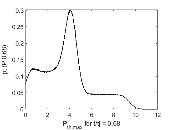
For each observer time , we run a Monte Carlo simulation drawing observing angles from a probability distribution. We then use the predicted polarization (Rossi et al. 2004) to derive the probability distribution of the observed polarization for . An example of the derived distributions is shown in Figure 3. By repeating this process for every observation we obtain a set of probability distributions, each associated with one polarization measurement. Under our assumption that all bursts are statistically drawn from a single population with only the viewing angle as a variable we can now evaluate a best value for our ratio that maximizes the probability of the measurement sample.
Let be the probability of measuring a polarization value within an interval around the value , for an observed time and , i.e., the maximum theoretical value. For a given we then have:
| (2) |
We therefore have that the log-likelihood of all our measurements sharing a single value of is given by:
| (3) |
where the index runs over all the measurements in Table 1. Note that the probability distributions are convolved with a Gaussian function with standard deviation equal to the uncertainty of the polarization measurements. This is done to smooth out sharp features in the theoretical probability distributions that could not be reproduced in a dataset that is affected by uncertainties.
| GRB | Ref() | Ref() | ||
|---|---|---|---|---|
| 990510 | 0.51 | 1.7 | Stanek et al. 1999 | Covino et al. 1999 |
| 0.57 | 1.6 | Wijers et al. 1999 | ||
| 020405 | 0.73 | 1.5 | Price et al. 2003 | Masetti et al. 2003 |
| 1.3 | 1.96 | Covino et al. 2003 | ||
| 1.9 | 1.47 | Covino et al. 2003 | ||
| 020813 | 3.08 | 1.07 | Lazzati et al. 2004 | Gorosabel et al. 2004 |
| 3.21 | 1.42 | Gorosabel et al. 2004 | ||
| 3.34 | 1.11 | Gorosabel et al. 2004 | ||
| 3.48 | 1.05 | Gorosabel et al. 2004 | ||
| 3.82 | 1.43 | Gorosabel et al. 2004 | ||
| 6.78 | 1.26 | Gorosabel et al. 2004 | ||
| 021004 | 0.13 | 0.51 | Holland et al. 2003 | Lazzati et al. 2003 |
| 0.14 | 0.71 | Rol et al. 2003 | ||
| 030328 | 1.54 | 2.4 | Maiorano et al. 2006 | Maiorano et al. 2006 |
| 080928 | 0.68 | 2.5 | Leventis et al. 2014 | Covino & Gotz 2016 |
| 091018 | 0.53 | 1.07 | Wiersema et al. 2012 | Wiersema et al. 2012 |
| 0.98 | 1.44 | Wiersema et al. 2012 | ||
| 2.46 | 1.73 | Wiersema et al. 2012 | ||
| 2.50 | 3.25 | Wiersema et al. 2012 | ||
| 2.53 | 1.99 | Wiersema et al. 2012 | ||
| 2.57 | 1.42 | Wiersema et al. 2012 | ||
| 3.01 | 0.97 | Wiersema et al. 2012 | ||
| 3.13 | 1.08 | Wiersema et al. 2012 | ||
| 5.16 | 1.45 | Wiersema et al. 2012 |
III. Results
The value of the log-likelihood as a function of the parameter is shown in Figure 4. We found that the value of with the maximum likelihood was
| (4) |
but a second high-probability peak is visible at . The red line in Figure 4 marks the confidence region and is obtained by allowing for a drop of in the log-likelihood below its best value. The most likely value of did not change significantly with a change in the assumed value of . The independence of the probability distribution on the assumed value of also ensures that our result would remain unaltered even if we assumed a probability distribution for the jet opening angle of different bursts.
The fact that maximizes the likelihood does not ensure that the model is consistent with the data. In order to verify this, we compare the distribution of measured polarization with the average of the individual distributions . The comparison is shown in Figure 5. A comparison of the predicted and observed polarization rates was done using the Kolmogorov-Smirnov test. This test resulted in a probability that the observed and model points came from the same distribution. As can be seen in Figure 5, there is a range between 2.5% and 6% polarization predicted in the model that is not accounted for in the observations.

To put our result in context, consider that the observed polarization is related to the ratio of the energy density of the parallel and perpendicular components of the magnetic field (Gruzinov & Waxman 1999; Sari 1999; Granot & Königl 2003)
| (5) |
through the equation:
| (6) |
which relates the observed polarization in a given direction with the one locally achievable in a fully ordered field for a viewer at a comoving angle from the shock normal. Since most of the radiation from a burst afterglow comes from a thin ring at (Panaitescu & Mészáros 1998; Granot et al. 1999), we simplify the equation as
| (7) |
after integration over the emitting surface. A more precise relationship between and would require a case-by-case integration over the emitting surface that is beyond the scope of this paper (see, e.g., Gill & Granot 2019). Note that the above equation predicts the possibility of negative polarization, which is impossible. Polarization sign, in this case, is used as an indication of the position angle of linear polarization. Polarization of opposite sign imply position angles orthogonal to each other. Since we cannot investigate position angle, our value of should be allowed to be negative as well as positive. We therefore find a double constraint on the geometry of the magnetic field:
| (8) |
and
| (9) |
where the first number corresponts to the most probable and the second to the secondary probability peak at . All values are consistent with the estimate obtained by Granot & Königl 2003. We notice that, in all cases, the perpendicular component of the field dominates: = 1.2 , 1.1 , 3.3 , and 3.7, respectively. An alternative parameterization was recently proposed by Gill & Granot 2019, who define the ratio as the amount of stretch of the field along the parallel direction with respect to an isotropic field (which would have ). They find that and our analysis therefore yields:
| (10) |

IV. Discussion
We have presented an analysis of the available ensemble of linear polarization measurements in the optical afterglow of long-duration gamma-ray bursts. The analysis is aimed at finding the ratio between the measured polarization and the maximum theoretically possible, which would be observed if the magnetic field would be either completely ordered parallel to the shock normal or entirely contained in the plane of the shock. The ratio is a proxy for the geometry of the magnetic field that can be quantified either through the parameter (Gruzinov & Waxman 1999; Sari 1999) or through the stretch parameter (Gill & Granot 2019).
We find that the available measurements are highly constraining of the polarization of the afterglows and, consequently, of the field geometry. We also find that our result is in some tension with the analysis of Gill & Granot 2019, who looked at the upper limit on the polarization of GW170817, a short gamma-ray burst for which the viewing geometry is known. However, several simplifying assumptions were made and significant systematic uncertainties are brought about by the choice of polarization model, outflow geometry, and jet dynamics. Here we discuss all these choices and approximations to inform the reader of their potential impact.
First, we chose to adopt a top hat jet for our polarization model. The rationale behind this choice is that it makes the probability of detection of an afterglow independent on the observer angle. This makes our calculation more straightforward and robust, since we do not have to assume a detection threshold, nor that all bursts are observed in the same way and with the same sensitivity. On the other hand, it seems likely that real GRB jets are structured, at least to some level (e.g., Granot & Kumar 2003; Kumar & Granot 2003; Rossi et al. 2004; Zhang et al. 2004; Morsony et al. 2007; Lazzati et al. 2018). Since the polarization curve for a structured jet is qualitatively different from that of a top-hat jet, our result would apply to that case only at the order of magnitude level. We note that Gill & Granot 2019 adopt a structured jet in their analysis, a difference that is most likely at the origin of the tension between the two results. An extension of this work to include structured jets is planned. As a matter of fact, the polarization measurements shown in Figure 2 do hint at a maximum of the measured polarization at about the jet break time, a feature that is characteristic of structured jets. Another hint that our jet model might be oversimplified can be gleaned from Figure 5. The figure shows how the models predict polarization of up to , which are not observed, yielding a low Kolmogorov-Smirnov probability (see Section III). Since the highest polarization is predicted for observers right on the edge of the jet, such prediction would be overestimated if the jet had a smooth transition, rather than an abrupt edge as implied by the top-hat model. In support of our choice, however, there are at least two bursts in which the rotation of the polarization angle that is characteristic of a top-hat jet has been observed: GRB091018 (Wiersema et al. 2012) and GRB121024A (which is, however, excluded from the sample due to the peculiarity of having significant circular polarization, Wiersema et al. 2014).
Another important choice we made was selecting the model of Rossi et al. 2004 as our fiducial model. Calculations by different authors differ in the details, and consequently there are differences in the order of a few tens of percent among the theoretical models (see, e.g., Granot et al. 2002). In addition, different assumptions on the sideways expansion dynamics cause different polarization, in some cases even adding to the complexity by causing a third peak to appear in the polarization curve (Sari 1999; Figure 5 in Rossi et al. 2004). To test the sensitivity of our results to the assumption on the sideways expansion, we repeated the analysis using the models in Figure 9 of Rossi et al. 2004, which assume that the jet expands sideways with relativistic speed of sound . We found a most probable value , associated with a lower KS probability . These significantly different values underline the sensitivity of polarization on poorly known dynamic properties of the outflows. We plan to address some of these uncertainties in future publications. Hopefully, additional data will then be available to further constrain the models and interpretations.
References
- Beloborodov (2011) Beloborodov, A. M. 2011, ApJ, 737, 68, doi: 10.1088/0004-637X/737/2/68
- Beloborodov (2013) —. 2013, ApJ, 764, 157, doi: 10.1088/0004-637X/764/2/157
- Björnsson et al. (2001) Björnsson, G., Hjorth, J., Jakobsson, P., Christensen, L., & Holland, S. 2001, ApJ, 552, L121, doi: 10.1086/320328
- Burgess et al. (2019) Burgess, J. M., Bégué, D., Greiner, J., et al. 2019, Nature Astronomy, 471, doi: 10.1038/s41550-019-0911-z
- Covino & Gotz (2016) Covino, S., & Gotz, D. 2016, Astronomical and Astrophysical Transactions, 29, 205. https://arxiv.org/abs/1605.03588
- Covino et al. (1999) Covino, S., Lazzati, D., Ghisellini, G., et al. 1999, A&A, 348, L1. https://arxiv.org/abs/astro-ph/9906319
- Covino et al. (2003) Covino, S., Malesani, D., Ghisellini, G., et al. 2003, A&A, 400, L9, doi: 10.1051/0004-6361:20030133
- Daigne & Mochkovitch (1998) Daigne, F., & Mochkovitch, R. 1998, MNRAS, 296, 275, doi: 10.1046/j.1365-8711.1998.01305.x
- Gendre et al. (2010) Gendre, B., Klotz, A., Palazzi, E., et al. 2010, MNRAS, 405, 2372, doi: 10.1111/j.1365-2966.2010.16601.x
- Ghirlanda et al. (2019) Ghirlanda, G., Salafia, O. S., Paragi, Z., et al. 2019, Science, 363, 968, doi: 10.1126/science.aau8815
- Ghisellini & Lazzati (1999) Ghisellini, G., & Lazzati, D. 1999, MNRAS, 309, L7, doi: 10.1046/j.1365-8711.1999.03025.x
- Giannios (2006) Giannios, D. 2006, A&A, 457, 763, doi: 10.1051/0004-6361:20065000
- Gill & Granot (2018) Gill, R., & Granot, J. 2018, MNRAS, 478, 4128, doi: 10.1093/mnras/sty1214
- Gill & Granot (2019) —. 2019, MNRAS, 2980, doi: 10.1093/mnras/stz3340
- Gorosabel et al. (2004) Gorosabel, J., Rol, E., Covino, S., et al. 2004, A&A, 422, 113, doi: 10.1051/0004-6361:20034409
- Granot & Königl (2003) Granot, J., & Königl, A. 2003, ApJ, 594, L83, doi: 10.1086/378733
- Granot & Kumar (2003) Granot, J., & Kumar, P. 2003, ApJ, 591, 1086, doi: 10.1086/375489
- Granot et al. (2002) Granot, J., Panaitescu, A., Kumar, P., & Woosley, S. E. 2002, ApJ, 570, L61, doi: 10.1086/340991
- Granot et al. (1999) Granot, J., Piran, T., & Sari, R. 1999, ApJ, 513, 679, doi: 10.1086/306884
- Greiner et al. (2003) Greiner, J., Klose, S., Reinsch, K., et al. 2003, Nature, 426, 157, doi: 10.1038/nature02077
- Gruzinov & Waxman (1999) Gruzinov, A., & Waxman, E. 1999, ApJ, 511, 852, doi: 10.1086/306720
- Holland et al. (2003) Holland, S. T., Weidinger, M., Fynbo, J. P. U., et al. 2003, AJ, 125, 2291, doi: 10.1086/374235
- Kumar & Granot (2003) Kumar, P., & Granot, J. 2003, ApJ, 591, 1075, doi: 10.1086/375186
- Lazzati et al. (2009) Lazzati, D., Morsony, B. J., & Begelman, M. C. 2009, ApJ, 700, L47, doi: 10.1088/0004-637X/700/1/L47
- Lazzati et al. (2013) Lazzati, D., Morsony, B. J., Margutti, R., & Begelman, M. C. 2013, ApJ, 765, 103, doi: 10.1088/0004-637X/765/2/103
- Lazzati et al. (2018) Lazzati, D., Perna, R., Morsony, B. J., et al. 2018, Phys. Rev. Lett., 120, 241103, doi: 10.1103/PhysRevLett.120.241103
- Lazzati et al. (2003) Lazzati, D., Covino, S., di Serego Alighieri, S., et al. 2003, A&A, 410, 823, doi: 10.1051/0004-6361:20031321
- Lazzati et al. (2004) Lazzati, D., Covino, S., Gorosabel, J., et al. 2004, A&A, 422, 121, doi: 10.1051/0004-6361:20035951
- Leventis et al. (2014) Leventis, K., Wijers, R. A. M. J., & van der Horst, A. J. 2014, MNRAS, 437, 2448, doi: 10.1093/mnras/stt2055
- Maiorano et al. (2006) Maiorano, E., Masetti, N., Palazzi, E., et al. 2006, A&A, 455, 423, doi: 10.1051/0004-6361:20054728
- Masetti et al. (2003) Masetti, N., Palazzi, E., Pian, E., et al. 2003, A&A, 404, 465, doi: 10.1051/0004-6361:20030491
- Mészáros & Rees (1997) Mészáros, P., & Rees, M. J. 1997, ApJ, 476, 232, doi: 10.1086/303625
- Mooley et al. (2018) Mooley, K. P., Deller, A. T., Gottlieb, O., et al. 2018, Nature, 561, 355, doi: 10.1038/s41586-018-0486-3
- Morsony et al. (2007) Morsony, B. J., Lazzati, D., & Begelman, M. C. 2007, ApJ, 665, 569, doi: 10.1086/519483
- Panaitescu & Mészáros (1998) Panaitescu, A., & Mészáros, P. 1998, ApJ, 493, L31, doi: 10.1086/311127
- Pe’er et al. (2005) Pe’er, A., Mészáros, P., & Rees, M. J. 2005, ApJ, 635, 476, doi: 10.1086/497360
- Pe’er et al. (2006) —. 2006, ApJ, 642, 995, doi: 10.1086/501424
- Price et al. (2003) Price, P. A., Kulkarni, S. R., Berger, E., et al. 2003, ApJ, 589, 838, doi: 10.1086/374730
- Rees & Meszaros (1994) Rees, M. J., & Meszaros, P. 1994, ApJ, 430, L93, doi: 10.1086/187446
- Rol et al. (2003) Rol, E., Wijers, R. A. M. J., Fynbo, J. P. U., et al. 2003, A&A, 405, L23, doi: 10.1051/0004-6361:20030731
- Rossi et al. (2002) Rossi, E., Lazzati, D., & Rees, M. J. 2002, MNRAS, 332, 945, doi: 10.1046/j.1365-8711.2002.05363.x
- Rossi et al. (2004) Rossi, E. M., Lazzati, D., Salmonson, J. D., & Ghisellini, G. 2004, MNRAS, 354, 86, doi: 10.1111/j.1365-2966.2004.08165.x
- Salmonson (2003) Salmonson, J. D. 2003, ApJ, 592, 1002, doi: 10.1086/375580
- Sari (1999) Sari, R. 1999, ApJ, 524, L43, doi: 10.1086/312294
- Sari & Piran (1997) Sari, R., & Piran, T. 1997, MNRAS, 287, 110, doi: 10.1093/mnras/287.1.110
- Sari et al. (1998) Sari, R., Piran, T., & Narayan, R. 1998, ApJ, 497, L17, doi: 10.1086/311269
- Stanek et al. (1999) Stanek, K. Z., Garnavich, P. M., Kaluzny, J., Pych, W., & Thompson, I. 1999, ApJ, 522, L39, doi: 10.1086/312219
- Tchekhovskoy et al. (2008) Tchekhovskoy, A., McKinney, J. C., & Narayan, R. 2008, MNRAS, 388, 551, doi: 10.1111/j.1365-2966.2008.13425.x
- van Eerten & MacFadyen (2013) van Eerten, H., & MacFadyen, A. 2013, ApJ, 767, 141, doi: 10.1088/0004-637X/767/2/141
- Vurm & Beloborodov (2016) Vurm, I., & Beloborodov, A. M. 2016, ApJ, 831, 175, doi: 10.3847/0004-637X/831/2/175
- Wiersema et al. (2012) Wiersema, K., Curran, P. A., Krühler, T., et al. 2012, MNRAS, 426, 2, doi: 10.1111/j.1365-2966.2012.20943.x
- Wiersema et al. (2014) Wiersema, K., Covino, S., Toma, K., et al. 2014, Nature, 509, 201, doi: 10.1038/nature13237
- Wijers et al. (1999) Wijers, R. A. M. J., Vreeswijk, P. M., Galama, T. J., et al. 1999, ApJ, 523, L33, doi: 10.1086/312262
- Zhang & Mészáros (2002) Zhang, B., & Mészáros, P. 2002, ApJ, 571, 876, doi: 10.1086/339981
- Zhang & Yan (2011) Zhang, B., & Yan, H. 2011, ApJ, 726, 90, doi: 10.1088/0004-637X/726/2/90
- Zhang et al. (2004) Zhang, W., Woosley, S. E., & Heger, A. 2004, ApJ, 608, 365, doi: 10.1086/386300