Adaptive Control Barrier Functions for Safety-Critical Systems
Abstract
Recent work showed that stabilizing affine control systems to desired (sets of) states while optimizing quadratic costs and observing state and control constraints can be reduced to quadratic programs (QP) by using control barrier functions (CBF) and control Lyapunov functions. In our own recent work, we defined high order CBFs (HOCBFs) to accommodating systems and constraints with arbitrary relative degrees, and a penalty method to increase the feasibility of the corresponding QPs. In this paper, we introduce adaptive CBF (AdaCBFs) that can accommodate time-varying control bounds and dynamics noise, and also address the feasibility problem. Central to our approach is the introduction of penalty functions in the definition of an AdaCBF and the definition of auxiliary dynamics for these penalty functions that are HOCBFs and are stabilized by CLFs. We demonstrate the advantages of the proposed method by applying it to a cruise control problem with different road surfaces, tires slipping, and dynamics noise.
I INTRODUCTION
Barrier functions (BFs) are Lyapunov-like functions [16][17], whose use can be traced back to optimization problems [5]. More recently, they have been employed to prove set invariance [4][14][18] and for multi-objective control [13]. In [16], it was proved that if a BF for a given set satisfies Lyapunov-like conditions, then the set is forward invariant. A less restrictive form of a BF, which is allowed to grow when far away from the boundary of the set, was proposed in [2]. Another approach that allows a BF to be zero was proposed in [8] [11]. This simpler form has also been considered in time-varying cases and applied to enforce Signal Temporal Logic (STL) formulas as hard constraints [11].
Control BFs (CBFs) are extensions of BFs for control systems, and are used to map a constraint that is defined over system states to a constraint on the control input. Recently, it has been shown that, to stabilize an affine control system while optimizing a quadratic cost and satisfying states and control constraints, CBFs can be combined with control Lyapunov functions (CLFs) [15][3][6][1] to form quadratic programs (QPs) [7][2][8] that are solved in real time.
The CBFs from [2] and [8] work for constraints that have relative degree one with respect to the system dynamics. A backstepping approach was introduced in [9] to address higher relative degree constraints, and it was shown to work for relative degree two. A CBF method for position-based constraints with relative degree two was also proposed in [19]. A more general form, which works for arbitrarily high relative degree constraints, was proposed in [12]. The method in [12] employs input-output linearization and finds a pole placement controller with negative poles to stabilize the CBF to zero. Thus, this CBF is an exponential CBF. The high order CBF (HOCBF) that we proposed in [20] is simpler and more general than the exponential CBF [12]. However, the QPs can easily be infeasible when both state constraints (enforced by HOCBFs) and tight control bounds are involved. Although the penalties involved in the definition of the HOCBF can help to improve feasibility [20], this might not work under time-varying control bounds and dynamics noise. In addition, the HOCBF method is conservative in the sense that the satisfaction of the HOCBF constraint is only sufficient for the satisfaction of the original constraint, which can limit the system performance.
To improve the problem feasibility under time-varying control bounds and dynamics noise, in this paper we propose adaptive CBFs (AdaCBFs). The proposed AdaCBFs can also help to alleviate the conservativeness of the HOCBF method. Specifically, we introduce penalty functions in the definition of an AdaCBF, and define auxiliary dynamics for these penalty functions that are HOCBFs (such that they are guaranteed to be non-negative) and are stabilized by CLFs. This way, the AdaCBF constraint is relaxed by the penalty functions through the control inputs of the auxiliary dynamics, while the forward invariance property of the HOCBF method is guaranteed. Since the AdaCBF constraint is relaxed through the penalty functions, we show that its satisfaction is a necessary and sufficient condition for the satisfaction of the original constraint, which leads to improvements in the performance of the system.
We formulate optimal control problems with constraints given by AdaCBFs and CLFs, and show the adaptivity of the proposed AdaCBF on an adaptive cruise control (ACC) problem with different and time-varying control bounds (e.g., on different road surfaces and with tires slipping), as well as with dynamics noise. The results clearly demonstrate the advantages of the proposed AdaCBF.
II PRELIMINARIES
Definition 1
(Class function [10]) A continuous function is said to belong to class if it is strictly increasing and .
Consider an affine control system of the form
| (1) |
where , and are globally Lipschitz, and ( denotes the control constraint set). Solutions of (1), starting at (we set the initial time to 0 without loss of generality), , are forward complete.
Suppose the control bound is defined as (the inequality is interpreted componentwise):
| (2) |
with .
Definition 2
A set is forward invariant for system (1) if its solutions starting at any satisfy for .
Definition 3
(Relative degree) The relative degree of a (sufficiently many times) differentiable function with respect to system (1) is the number of times we need to differentiate it along its dynamics until the control explicitly shows in the corresponding derivative.
In this paper, since function is used to define a constraint , we will also refer to the relative degree of as the relative degree of the constraint.
For a constraint with relative degree , , and , we define a sequence of functions :
| (3) |
where denotes a order differentiable class function.
We further define a sequence of sets associated with (3) in the form:
| (4) |
Definition 4
(High Order Control Barrier Function (HOCBF) [20]) Let be defined by (4) and be defined by (3). A function is a high order control barrier function (HOCBF) of relative degree for system (1) if there exist order differentiable class functions and a class function such that
| (5) |
for all . In (5), () denotes Lie derivatives along () (one) times, denotes the remaining Lie derivatives along with degree less than or equal to (omitted for simplicity, see [20]).
The HOCBF is a general form of the relative degree one CBF [2] [8] [11] (set in the HOCBF, and we can show that the CBF form in [2] is the same as [8] [11]), and it is also a general form of the exponential CBF [12] for high relative degree constraints (define all the class functions in linear form in Def. 4).
Given a HOCBF , we define the set of all control values that satisfy (5) as:
| (6) | |||
Theorem 1
Definition 5
Theorem 2
Note that (8) can be relaxed by replacing 0 with a relaxation variable at its right-hand side, and we wish to minimize this relaxation variable [1]. Recent works [2], [11], [12] combine CBFs and CLFs with quadratic costs to form optimization problems. Time is discretized and an optimization problem with constraints given by CBFs and CLFs is solved at each time step. Note that these constraints are linear in control since the state is fixed at the value at the beginning of the interval, and therefore the optimization problem is a quadratic program (QP). The optimal control obtained by solving the QP is applied at the current time step and held constant for the whole interval. The dynamics (1) are updated, and the procedure is repeated. This method works conditioned on the fact that the QP at every time step is feasible. However, this is not guaranteed, in particular under tight control bounds. In this paper, we show how the QP feasibility can be improved by using adaptive CBFs.
III ADAPTIVE CONTROL BARRIER FUNCTIONS
In this section, we define adaptive CBFs (AdaCBFs). We use a simple example to motivate the need for such functions and to illustrate the main ideas.
III-A Example: Simplified Adaptive Cruise Control
Consider the simplified adaptive cruise control (SACC) problem11 1 A more realistic version of this problem, called the adaptive cruise control problem (ACC), is defined in Sec. IV. with the ego (controlled) vehicle dynamics in the form:
| (9) |
where and denote the position and velocity of the controlled vehicle along its lane, respectively, and is its control.
We also have control constraints:
| (10) |
where and are the minimum and maximum control input, respectively.
We require that the distance between the ego vehicle and its immediately preceding vehicle (the coordinates of the ego vehicle and of the preceding vehicle, respectively, are measured from the same origin and ) be greater than , i.e.,
| (11) |
Assume the preceding vehicle runs at constant speed . Let and . The relative degree of is 2, so we choose a HOCBF with . We define , and in Def. 4 and find a control for the ego vehicle such that the constraint (11) is satisfied. The control should satisfy:
| (12) | |||
Suppose we wish to minimize . We can then use the QP based method introduced at the end of the last section to solve this SACC problem. However, the HOCBF constraint (12) can easily conflict with in (10) when the two vehicles get close to each other, as shown in [20]. When this happens, the QP will be infeasible. We can use the penalty method from [20] to improve the QP feasibility, i.e., by adding a positive constant penalty on both . Then the control should satisfy:
| (13) | |||
Given , we can find a small enough value for such that (13) will not conflict with in (10), i.e., the QP is always feasible. However, the lower bound of the control is not a constant in reality. The value of depends on the weather condition and the road surface roughness, etc.. For example, the vehicle maximum braking force (directly corresponding to ) in a rainy day is usually smaller than the one in a sunny day. When we choose a proper for the HOCBF constraint (13) in the sunny day such that the QP in the SACC problem is always feasible, the QP may be infeasible in the rainy day. The unknown roughness of the road surface can further make the choice of the value difficult. Moreover, the assumption of a constant speed for the front vehicle is too strong, and there are also vehicle dynamics noise that could make the QP infeasible. This motivates us to define an AdaCBF that works for time-varying control bounds and dynamics noise (i.e., the QP is always feasible).
III-B Adaptive Control Barrier Function (AdaCBF)
We consider a function that defines an invariant set for system (1). For a relative degree function , let . Instead of using a constant penalty for each class function for the penalty method [20] in the definition of a HOCBF, we define as a penalty function of time and multiply it to each class function , respectively. Let . Thus, we define a sequence of functions in the form:
| (14) | ||||
where is a order differentiable class function, is a class function.
The remaining question is how to choose . As shown in the definition of a HOCBF, will be differentiated times, while with not be differentiated (so we can just set as a variable). Let where denotes a new defined state variable that will be used later ( is a single variable, and we need to differentiate it once). We define input-output linearizable auxiliary dynamics (take as the output with relative degree ) for each (we skip the time variable from now on for simplicity) in the form:
| (16) | ||||
where , denotes the control input for the auxiliary dynamics (16). Note that the auxiliary dynamics (16) are defined in general form. For simplicity, we can just define the auxiliary dynamics (16) in linear form. For example, we define (since we need to differentiate twice as shown in Def. 4), and define (since we need to differentiate once). Theoretically, we can initialize to any real number vector as long as .
Definition 6
Let be defined by (15), be defined by (14), and the auxiliary dynamics be defined by (16). A function is an adaptive control barrier function (AdaCBF) with relative degree for (1) if every is a HOCBF with relative degree for the auxiliary dynamics (16), and there exist order differentiable class functions , a class function such that
| (17) | |||
for all , and all . In (17), denotes the remaining Lie derivative terms of (or ) along (or ) with degree less than (or ). These terms are skipped for simplicity but examples can be found in the revisited example or in the next section.
Let , where comes from the auxiliary dynamics (16). Note that is constrained by the HOCBF constraints (defined in the following constraint set) for each since is a HOCBF with relative degree for (16). We define a constraint set for in the form:
| (18) | |||
where is defined in (3) by replacing with .
Given an AdaCBF , we consider all control values that satisfy:
| (19) | |||
Theorem 3
Proof:
If is an AdaCBF, then we have that . Constraint (17) is equivalent to . If , it follows from Thm. 1 that . If , then . Since (i.e., is initially satisfied), we have that . Because is a HOCBF for the auxiliary dynamics (16), we have from Thm. 1 that . Then, we can recursively prove that similarly to the case , and eventually prove that , i.e., . Therefore, the sets and are forward invariant. ∎
Remark 1
In the AdaCBF constraint (17), the control input of system (1) depends on the control input of the auxiliary dynamics (16). The control input is only constrained by the corresponding HOCBF constraint (shown in (18)) since we require that is a HOCBF, and there are no control bounds on . Therefore, we somewhat relax the constraints on the control input of system (1) in the AdaCBF by allowing the penalty function to change. However, the forward invariance of the set is guaranteed, i.e., the original constraint is guaranteed to be satisfied. This is the adaptivity of the AdaCBF. Note that we may not need to define a penalty function for every class function in (14)-we can just define penalty functions for some of them.
Adaptivity to changing control bounds and dynamics noise: In the HOCBF method, the problem may be infeasible in the presence of both control limitations (2) and the HOCBF constraint (5). There are two reasons for the problem to become infeasible: the control limitations (2) are too tight or the control limitations are time-varying such that the HOCBF constraint (5) will conlict with (2) after it becomes active; the dynamics (1) are not accurately modeled, and there may be uncertain variables, etc. (we consider all of them as dynamics noise). In this case, the HOCBF constraint (5) might also conlict with (2) when both of them become active. This is because the state variables also show up in the HOCBF constraint (5), and thus, the dynamics noise can easily (and randomly) change the HOCBF constraint (5) through the (noised) state variables such that (5) may conflict with the control limitations when they are also active. However, the problem feasibility is improved in the AdaCBF method since the control in the AdaCBF constraint (17) is relaxed by , as discussed in Remark 1. In order to make the original constraint not be violated by the noise, we can define high order class functions (such as high order polynomials) such that the value of the AdaCBF will stay away from 0 in the long run after the corresponding AdaCBF constraint (17) becomes active, as shown in [20].
Theorem 4
Proof:
If , it follows from Thm. 3 that we can always choose proper class functions (such as linear functions, quadratic functions, etc.) such that and (note that ). Thus, the satisfaction of the AdaCBF constraint (17) is a sufficient condition for the satisfaction of the original constraint .
If , we have that there exists a penalty function (since is a HOCBF) such that for any with respect to dynamics (1) (because ). Note from (14) that , we have (i.e., ). The derivative of shows in , and we can also prove similarly that there exists a penalty function (since is a HOCBF) such that in a recursive way. Eventually, there exists such that (i.e., ). Since is equivalent to the satisfaction of the AdaCBF constraint (17), we have that the satisfaction of the AdaCBF constraint (17) is a necessary condition for the satisfaction of the original constraint . ∎
Remark 2
Since is required to be order differentiable, it is usually not guaranteed to find such functions when we find the control by solving the QPs introduced at the end of Sec. II. Since the satisfaction of the AdaCBF constraint (17) is equivalent to the satisfaction of the original constraint, the system performance is not reduced in the mapping of a constraint from state to control.
Example revisited. For the SACC problem introduced in Sec.III-A, the relative degree of the constraint from Eqn. (11) is 2, i.e., we need an AdaCBF with . We still choose and in the definition of an AdaCBF in Def. 6. Suppose we only consider a penalty function on the class function and define linear dynamics for in the form . In order for to be an AdaCBF for (9), a control input should satisfy
| (20) | |||
Since depends on that is without control bounds, the control input in the above AdaCBF constraint is relaxed. Thus, this constraint is adaptive to the change of the control bound in (10) and the uncertainties of and from the front vehicle, etc.. Note that should be a HOCBF for the auxiliary dynamics . The control input is constrained by the corresponding HOCBF constraint such that is satisfied.
III-C Optimal Control with AdaCBFs
Consider an optimal control problem for system (1) with the cost defined as:
| (21) |
where denotes the 2-norm of a vector, is a strictly increasing function of its argument, and .
System (1) is not accurately modeled, as well as is with uncertain variables (both are unknown, and we can assign uncertain variables with the values of measured expection). In addition, system (1) has time-varying control bound defined as:
| (22) |
with .
Assume a (safety) constraint with relative degree has to be satisfied by system (1). In order to improve the problem feasibility, we use the AdaCBF method. Then should satisfy the AdaCBF constraint (17). Moreover, each is constrained by the HOCBF constraint (5) corresponding to the constraint for the auxiliary dynamics (16).
Note that the control from the auxiliary dynamics are without control bounds, and are only constrained by the HOCBF constraints defined in (18). However, the HOCBF constraint for each is only constrained from one side, i.e.,
| (23) |
if . Therefore, is unbounded in the (positive) infinity side. The adaptivity of an AdaCBF depends on the auxiliary dynamics (16) (i.e., depends on ). If changes too fast, it can affect the smoothness of the control obtained through solving the QPs, and thus, may damage the performance of system (1).
If we add control bounds on , the problem feasibility may be decreased (i.e., the adaptivity of an AdaCBF is weakened). If we try to minimize each in the cost, may stay at a large value, which contradicts with the penalty method from [20] (i.e., we wish to have small enough value of to improve the problem feasibility). Therefore, we wish to stabilize the values of and always try to decrease when it is large. We usually stabilize each to a small enough value (recommended by the penalty method from [20] or by the optimal penalties learned in [21]). We choose smaller if is a high order function (such as polynomial function) than a low order one. Suppose the auxiliary dynamics (16) are input-output linearized (otherwise, we can do input-output linearization as we have assumed that (16) is input-output linearizable), we can use either the tracking control from [10] or the CLF method to stabilize , i.e., if , we wish to minimize (take as a decision variable), if , we define a CLF as in Def. 5, and if , we find a desired state feedback for in the form:
| (24) |
where . In the last equation, if , we can directly define a CLF as in Def. 5.
Then we can define a CLF (the relative degree of is one) to stabilize each with in Def. 5, any control input should satisfy:
| (25) |
where denotes a relaxation variable that we want to minimize.
In all cases, we may also want to stabilize that is not differentiated, we can just minimize (take as a decision variable). As discussed in the above, we wish to decrease when it is large, so we always want to minimize . Therefore, we can reformulate the cost (21) by the AdaCBF in the form (let ):
| (26) | |||
subject to (1), (22), (17), (16), the HOCBF constraint in (18) for each , , and the CLF constraint (25). , and .
Complexity: The time complexity of QP (active-set method) is polynomial in the dimension of decision variables on average. In general, the complexity is , where denotes the dimension of the decision variable space. In the HOCBF based QP, the complexity is (recall that is the dimension of the control ). However, in (26), the complexity becomes . We increase the adaptivity of the CBF method at the cost of more computation time, but the AdaCBF based QP is still fast enough in most problems, as we will see in the simulations.
IV ACC PROBLEM FORMULATION
In this section, we consider a more realistic version of the adaptive cruise control (ACC) problem introduced in Sec.III-A, which was referred to as the simplified adaptive cruise control (SACC) problem. we consider that the safety constraint is critical and study the adaptivity of AdaCBF discussed in the last section.
Vehicle Dynamics: Instead of using the simple dynamics in (9), we consider more accurate vehicle dynamics in the form:
| (27) |
where denotes the mass of the controlled vehicle. denotes the resistance force, which is expressed [10] as:
| (28) |
where and are scalars determined empirically. The first term in denotes the coulomb friction force, the second term denotes the viscous friction force and the last term denotes the aerodynamic drag.
Constraint 1 (Vehicle limitations): There are constraints on the speed and acceleration, i.e.,
| (29) | |||
where and denote the maximum and minimum allowed speeds, while and are deceleration and acceleration coefficients, respectively, and is the gravity constant.
Constraint 2 (Safety): Eqn. (11).
Objective 1 (Desired Speed): The controlled vehicle always attempts to achieve a desired speed .
Objective2 (Minimum Energy Consumption): We also want to minimize the energy consumption:
| (30) |
Problem 1
Determine control laws to achieve Objectives 1, 2 subject to Constraints 1, 2, for the controlled vehicle governed by dynamics (27).
V ACC PROBLEM REFORMULATION
For Problem 1, we use the quadratic program (QP) - based method introduced in [2]. The relative degree of (11) is 2, so we defined an AdaCBF with . We consider a quadratic class function for and a linear class function for in the definition of the AdaCBF.
V-A Desired Speed (Objective 1)
V-B Vehicle Limitations (Constraint 1)
The relative degrees of speed limitations are 1, we use HOCBFs with to map the limitations from speed to control input . Let , and choose in Def. 4 for both HOCBFs. Then any control input should satisfy
| (32) |
| (33) |
Since the control limitations are already constraints on control input, we do not need HOCBFs for them.
V-C Safety Constraint (Constraint 2)
Since the HOCBF constraint for (11) can easily conflict with the control limitations in (29), we use an AdaCBF with (the relative degree of the safety constraint (11) is two). Let , we define in the form:
| (34) | ||||
We define an auxiliary dynamics for (we will not take derivatives on , so we just set as a decision variable to be determined (also time-varying)) in the form
| (35) |
Combining the dynamics (27) with (34), any control input should satisfy (the AdaCBF constraint):
| (36) | |||
Since has to be a HOCBF (), and its relative degree is 1 for (35), any control input should satisfy (define as in a linear function in Def. 4):
| (37) |
with .
We wish to stabilize to a desired (usually a small number), and define a CLF , with and in Def. 5. Any control input should satisfy:
| (38) |
Note that we may also wish to minimize , where .
V-D Reformulated ACC Problem
We partition the time interval into a set of equal time intervals , where . In each interval (), we assume the control is constant (i.e., the overall control will be piece-wise constant), and reformulate (approximately) Problem 1 as a sequence of QPs. Specifically, at (), we solve
| (39) |
where (We also assume is a constant vector in each interval), subject to
where the constraint parameters are
Remark 3
The control bound is usually not a constant (the same for , but it does not make sense to change since the AdaCBF constraint (36) can only conflict with ). We can also add noise to (27) as the AdaCBF constraint (36) is relaxed by , and thus is adaptive to the change of the control bound and dynamics noise.
VI IMPLEMENTATION AND RESULTS
In this section, we present case studies for Problem 1 to illustrate the adaptive property of the AdaCBF described in Sec.III.
All simulations were conducted in MATLAB. We used quadprog to solve the QPs and ode45 to integrate the dynamics. The parameters are listed in Table I. If we apply HOCBF implement the safety constraint (11) with , the QP will be infeasible after the corresponding HOCBF constraint becomes active. Therefore, we need the AdaCBF to implement this safety constraint, as shown next.
| Parameter | Value | Units | Parameter | Value | Units |
|---|---|---|---|---|---|
| 20 | 100 | ||||
| 13.89 | 24 | ||||
| 1650 | g | 9.81 | |||
| 0.1 | 5 | ||||
| 0.25 | 10 | ||||
| 30 | 0 | ||||
| 0.1 | 10 | unitless | |||
| TBD | unitless | 0.4 | unitless | ||
| 1 | unitless | 2 | unitless | ||
| unitless | unitless |
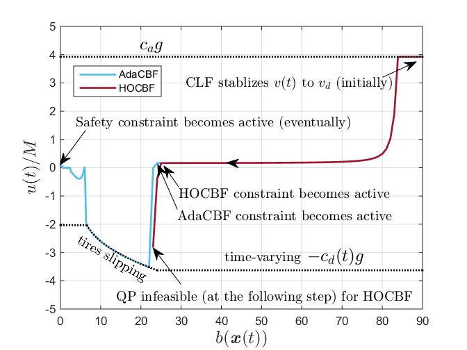
Adaptivity to the changing control bound : We first studies what happens when we change the lower control bound . In each simulation trajectory, we set the lower control bound coefficient to a different constant or to be time-varying (such as linearly decrease ). In this case, we set . We first present a case study of linearly decreasing (for example, due to tires slipping), as shown in Fig. 1. When we decrease (weaken the braking capability of the vehicle) after the HOCBF constraint becomes active, the QPs can easily become infeasible in the HOCBF method, as the red line shown in Fig. 1. In the AdaCBF method, the QPs are always feasible as shown in Fig. 1, which shows the adaptivity of the AdaCBF to the time-varying control bound (wheels slipping). The computational time at each time step for both the HOCBF and AdaCBF methods are less than in MATLAB (Intel(R) Core(TM) i7-8700 CPU @ 3.2GHz). Note that there is an over-shot for the control when is small, we can put more weight on control or decrease the weights to alleviate this overshot after the control constraint is not active, as the light blue curve shown in Fig. 2. The simulation trajectories for different (constant) values (for example, on different road surfaces) are shown in Figs. 2 and 3.
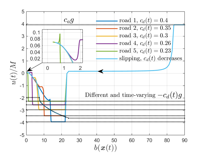

As shown in Fig. 2, when we set , the QP itself has good feasibility. This induces only a little change on the penalty varible and no change on , as shown in Fig. 3. As we decrease to a smaller one in another simulation (i.e., limit the braking capability of the vehicle), the variation of the penalty varibale becomes large after the AdaCBF constraint (36) becomes active. As we decrease to , the vehicle needs to brake with almost all the way to the safety constraint (11) becoming active, as green curves shown in Figs. 2 and 3. This value is close to the vehicle limit (i.e., only brake with the maximum braking force) such that the safety constraint can be satisifed. On the other hand, the penalty functions both change to a big value, as shown in Fig. 3. If we further decrease , the safety constraint (11) will be violated. The value change of the penalty functions demonstrates the adaptivity of the AdaCBF to the change of the control bound. The penalty method [20] shows that we wish to have smaller panelties to improve the QP feasibility before the HOCBF constraint becomes active, but the AdaCBF shows that we may actually want to increase the value of the penalties after the AdaCBF constraint becomes active, as the last frame shown in Fig. 3. This is also demonstrated on another example shown next.
Suppose we decrese from to , and we want to compare the minimum we can take beween them, as well as study what happens when we disable the penalty function in the AdaCBF, i.e., fix to a constant value. Simulation results are shown in Figs. 4 and 5.
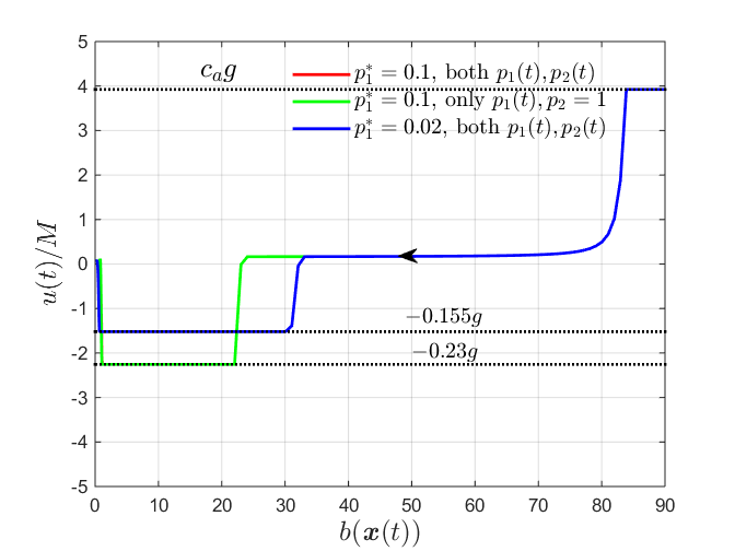

We can see that when we set to a constant instead of a penalty value, the control input profiles are almost the same, but require bigger values after the AdaCBF constraint (36) becomes active. When we decrease from to , we can further decrease to 0.155, as shown in Figs. 4 and 5. This is consistent with the penalty method [20] that we wish to take smaller penalties before the CBF constraint becomes active.
Adaptivity to dynamics noise: Suppose we add two noise terms to the speed and acceleration in dynamics (27), respective, where denote two random processes defined in an appropriate probability space. In the simulation, randomly take values in and with equal probability at time , respectively. We fix the value of to 0.23 in (29) and set . The simulation results under different noise levels are shown in Figs. 6 and 7, the noise is based on and for , respectively.


When the control constraint is active on , it can easily conflict with the HOCBF constraint (if we apply the HOCBF method) that is subjected to noise (which may make the safety constraint (11) violated if we apply the last moment control afterwards, as the blue line shown in Fig. 7), but the AdaCBF constraint is relaxed by the penalty functions (through ) and , and thus is adaptive to different dynamics noise levels and can make the QPs feasible, as shown in Fig. 6. The forward invariance of and is shown in Fig. 7. Note that might be temporarily negative due to noise during simulation, but will be positive again soon. This is due to the definition of in (34). When we have , the AdaCBF constraint ensures , and thus, (since ). Therefore, will be increasing and eventually becomes positive. In this paper, we consider high order polynomial class functions to make stay away from zero [20] (for example, we define as a quadratic function in (34)) such that is guaranteed in the presence of noise. The forward invariance gurantee can also be achieved by considering the noise bounds in the AdaCBF constraint. We will compare these two approaches in future work. Note that we can also define as a quadratic function in the definition of the AdaCBF in (34) to make also stay away from 0 in Fig. 7, and define as a higher order polynomial function to make the AdaCBF stay further away to 0, and thus it can be adaptive (in the sense of both QP feasibility and forward invariance) to higher noise levels.
VII CONCLUSION & FUTURE WORK
We introduce adaptive control barrier functions that can accommodate time-varying control bounds and dynamics noise, and also address the feasibility problem in this paper. The proposed adaptive control barrier function can also alleviate the conservativeness of the control barrier function method, and thus improve the system performance. We demonstrate the advantages of the proposed adaptive control barrier function by applying it to an adaptive cruise control problem. In the future, we will apply the adaptive control barrier function method to complex problems and systems.
References
- [1] Aaron D. Ames, K. Galloway, and J. W. Grizzle. Control lyapunov functions and hybrid zero dynamics. In Proc. of 51rd IEEE Conference on Decision and Control, pages 6837–6842, 2012.
- [2] Aaron D. Ames, Jessy W. Grizzle, and Paulo Tabuada. Control barrier function based quadratic programs with application to adaptive cruise control. In Proc. of 53rd IEEE Conference on Decision and Control, pages 6271–6278, 2014.
- [3] Zvi Artstein. Stabilization with relaxed controls. Nonlinear Analysis: Theory, Methods & Applications, 7(11):1163–1173, 1983.
- [4] Jean Pierre Aubin. Viability theory. Springer, 2009.
- [5] Stephen P Boyd and Lieven Vandenberghe. Convex optimization. Cambridge university press, New York, 2004.
- [6] R. A. Freeman and P. V. Kokotovic. Robust Nonlinear Control Design. Birkhauser, 1996.
- [7] K. Galloway, K. Sreenath, A. D. Ames, and J.W. Grizzle. Torque saturation in bipedal robotic walking through control lyapunov function based quadratic programs. preprint arXiv:1302.7314, 2013.
- [8] P. Glotfelter, J. Cortes, and M. Egerstedt. Nonsmooth barrier functions with applications to multi-robot systems. IEEE control systems letters, 1(2):310–315, 2017.
- [9] Shao-Chen Hsu, Xiangru Xu, and Aaron D. Ames. Control barrier function based quadratic programs with application to bipedal robotic walking. In Proc. of the American Control Conference, pages 4542–4548, 2015.
- [10] Hassan K. Khalil. Nonlinear Systems. Prentice Hall, third edition, 2002.
- [11] L. Lindemann and D. V. Dimarogonas. Control barrier functions for signal temporal logic tasks. IEEE Control Systems Letters, 3(1):96–101, 2019.
- [12] Quan Nguyen and Koushil Sreenath. Exponential control barrier functions for enforcing high relative-degree safety-critical constraints. In Proc. of the American Control Conference, pages 322–328, 2016.
- [13] D. Panagou, D. M. Stipanovic, and P. G. Voulgaris. Multi-objective control for multi-agent systems using lyapunov-like barrier functions. In Proc. of 52nd IEEE Conference on Decision and Control, pages 1478–1483, Florence, Italy, 2013.
- [14] Stephen Prajna, Ali Jadbabaie, and George J. Pappas. A framework for worst-case and stochastic safety verification using barrier certificates. IEEE Transactions on Automatic Control, 52(8):1415–1428, 2007.
- [15] E. Sontag. A lyapunov-like stabilization of asymptotic controllability. SIAM Journal of Control and Optimization, 21(3):462–471, 1983.
- [16] Keng Peng Tee, Shuzhi Sam Ge, and Eng Hock Tay. Barrier lyapunov functions for the control of output-constrained nonlinear systems. Automatica, 45(4):918–927, 2009.
- [17] Peter Wieland and Frank Allgower. Constructive safety using control barrier functions. In Proc. of 7th IFAC Symposium on Nonlinear Control System, 2007.
- [18] Rafael Wisniewski and Christoffer Sloth. Converse barrier certificate theorem. In Proc. of 52nd IEEE Conference on Decision and Control, pages 4713–4718, Florence, Italy, 2013.
- [19] Guofan Wu and Koushil Sreenath. Safety-critical and constrained geometric control synthesis using control lyapunov and control barrier functions for systems evolving on manifolds. In Proc. of the American Control Conference, pages 2038–2044, 2015.
- [20] Wei Xiao and Calin Belta. Control barrier functions for systems with high relative degree. In Proc. of 58th IEEE Conference on Decision and Control, pages 474–479, Nice, France, 2019. available in arXiv:1903.04706.
- [21] Wei Xiao, Calin Belta, and Christos G. Cassandras. Feasibility guided learning for robust control in constrained optimal control problems. In preprint in arXiv:1912.04066, 2019.