跳到论文正文
W Papers独立论文阅读器 arXiv:2002.04457 论文正文 计算阅读时间 · 0%
引用这篇论文根据当前论文元数据生成,正式投稿前建议核对。


License: arXiv.org perpetual non-exclusive license
arXiv:2002.04457v1 [cs.SI] 10 Feb 2020

Community Detection on Mixture Multi-layer Networks via Regularized Tensor Decomposition

Bing-Yi Jing    Ting Li    Zhongyuan Lyu    Dong Xia Affiliation: Hong Kong University of Science and Technology
(August 11, 2026)
Abstract

We study the problem of community detection in multi-layer networks, where pairs of nodes can be related in multiple modalities. We introduce a general framework, i.e., mixture multi-layer stochastic block model (MMSBM), which includes many earlier models as special cases. We propose a tensor-based algorithm (TWIST) to reveal both global/local memberships of nodes, and memberships of layers. We show that the TWIST procedure can accurately detect the communities with small misclassification error as the number of nodes and/or number of layers increases. Numerical studies confirm our theoretical findings. To our best knowledge, this is the first systematic study on the mixture multi-layer networks using tensor decomposition. The method is applied to two real datasets: worldwide trading networks and malaria parasite genes networks, yielding new and interesting findings.

11footnotetext: Jing and Li’s research is partially supported by the Hong Kong RGC Grants GRF 16304419 and GRF 16305616. Lyu and Xia’s research is partially supported by the Hong Kong RGC Grant ECS 26302019 and WeBank-HKUST project WEB19EG01-g.

1 Introduction

Networks arise in many areas of research and applications, which come in all shapes and sizes. The most studied and best understood are static network models. Many other network models are also in existence, but have been less studied. One such example is the multi-layer networks, which are a powerful representation of relational data, and commonly encountered in contemporary data analysis (Kivelä et al. 2014). The nodes in a multi-layer network represent the entities of interest and the edges in different layers indicate the multiple relations among those entities. Examples include brain connectivity networks, world trading networks, gene-gene interactive networks and so on. In this paper, we focus on the multi-layer networks with the same nodes set of each layer and there are no edges between two different layers.

The study on multi-layer networks has received an increasing interest. Considering the dependency among the different layers, Paul and Chen 2016 derives consistency results for the community assignments from the maximum likelihood estimators in two models. Consistency properties of various methods for community detection under the multi-layer stochastic block model are investigated in Paul and Chen 2017. Three different matrix factorization-based algorithms are employed in Tang et al. 2009, Nickel et al. 2011 and Dong et al. 2012 separately. Common community structures for multiple networks are identified via two spectral clustering algorithms with theoretical guarantee in Bhattacharyya and Chatterjee 2018. In Arroyo et al. 2019, authors introduce the common subspace independent-edge multiple random graph model to describe a heterogeneous collection of networks with a shared latent structure and propose a joint spectral embedding of adjacency matrices to simultaneously and consistently estimate underlying parameters for each graph. Consistency results for a least squares estimation of memberships under the multi-layer stochastic block model framework are derived in Lei et al. 2019. Several literature focus on recovering the network from a collection of networks with edge contamination. The original network is estimated from multiple noisy realizations utilizing community structure in Le et al. 2018 and low-rank expectation in Levin et al. 2019. A weighted latent position graph model contaminated via an edge weight gross error model is proposed in Tang et al. 2017 with an estimation methodology based on robust LqL_{q} estimation followed by low-rank adjacency spectral decomposition.

In applications, a random effects stochastic block model is proposed by Paul and Chen 2018 for the neuroimaging data and a statistical framework with a significance and a robustness test for detecting common modules in the Drosophila melanogaster dynamic gene regulation network is proposed in Zhang and Cao 2017.

Most of the literature about community detection in multi-layer networks is limited to consistent membership setting, which means all the layers carry information about the same community assignment. However, in reality, different layers may have different community structures. For instance, in a social network, layers related with sports (people connected with the same sport hobbies) may have different community structure with layers about movie taste (people connected with similar movie taste). Understanding the large-scale structure of multi-layer networks is made difficult by the fact that the patterns of one type of link may be similar to, uncorrelated with, or different from the patterns of another type of link. These differences from layer to layer may exist at the level of individual links, connectivity patterns among groups of nodes, or even the hidden groups themselves to which each node belongs. In De Bacco et al. 2017, authors pointed out that, in order to do community detection on multi-layer networks, it is crucial to know which layers have related structure and which layer are unrelated, since redundant information across layers may provide stronger evidence for clear communities than each layer would on its own. Such situation is not clearly discussed in the works mentioned above. Although, in Matias and Miele 2017, authors introduced community structure variety as time varying, it is hard to be applied in general multi-layer networks without time ordering.

In this paper, we introduce a general framework, i.e., mixture multi-layer stochastic block model (MMSBM), and propose a tensor-based algorithm (TWIST) to reveal both global/local memberships of nodes, and memberships of layers. To fix ideas, we start with a simple motivating example, illustrated in Figure 1. We have L=3L=3 layers of networks {𝒢1,𝒢2,𝒢3}\{{\cal G}_{1},{\cal G}_{2},{\cal G}_{3}\}, each containing 3 local communities. The 3 networks are of m=2m=2 types: {𝒢2}\{{\cal G}_{2}\} and {𝒢1,𝒢3}\{{\cal G}_{1},{\cal G}_{3}\}. The community structure differs between {𝒢2}\{{\cal G}_{2}\} and the other two networks as some members in the third community g23g_{23} are in the second one g12g_{12} in {𝒢1}\{{\cal G}_{1}\} and {𝒢3}\{{\cal G}_{3}\}. Viewing the 3 layers of networks together, we notice that there are 4 global communities, in which members stay in all layers throughout. Clearly, the global communities are related to, but different from the local ones in each network. Our interest lies in detecting both local as well as global community structures, which are of great value in theory and practice. There is an increasing literature on the global community structure as mention earlier. However, to the best of our knowledge, there is no systematic investigation into detecting local and global community structure together.

Refer to caption
Figure 1: A toy example.

Our line of attack can be illustrated via the following diagram in Figure 2. First, we pool adjacency matrices from all layers of networks to form a tensor (multi-way array), and then apply the TWIST (to be introduced later) to obtain the global community structure as well as labels of each layer. We then group the layers of networks with the same labels, which will be used to detect local community structures. Details will be unfolded next.
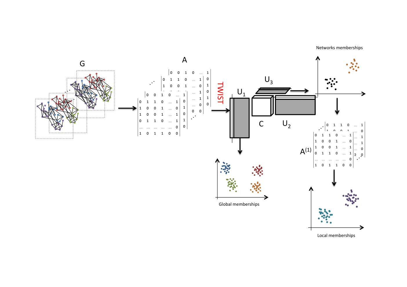
Refer to caption
Figure 2: The general procedure of TWIST.

The main contributions of this paper are summarized as follows.

First, we propose a very general model to handle the type of problems discussed above. To be more specific, we will introduce the so-called mixture multi-layer stochastic block model (MMSBM), which can characterize the different community structures among different layers of the multi-layer network. In some way, the MMSBM resembles the relatively well studied multi-layer stochastic block model (MLSBM) Paul and Chen 2017; Han et al. 2015; Paul and Chen 2016. However, the MMSBM is more general in that it allows the multi-layer network to contain different block structures. Thus, the MMSBM not only allows each layer to have different community structures, but also can maintain the consistent structure in the network.

Secondly, we propose a tensor-based method to study the MMSBM. The approach is referred to as the Tucker decomposition with integrated SVD transformation (TWIST). Unlike earlier approaches for multi-layer network analysis, TWIST can uncover the clusters of layers, the local and global membership of nodes simultaneously. On the theoretical front, we prove for MMSBM that TWIST can consistently recover the layer labels and global memberships of nodes under near optimal network sparsity conditions. In addition, network labels can be exactly recovered under a slightly stronger network sparsity condition. To the best of our knowledge, this is the first systematic study on statistical guarantees about community detection in a mixture multi-layer networks using tensor decomposition. Our primary technical tool is a sharp concentration inequality of sparse tensors which might be of independent interest.

Finally, two real-world applications of the proposed methodology demonstrated to be a powerful tool in analysing multi-layer networks. The algorithm is easy to use and can help practitioners quickly uncover interesting findings, which would otherwise be difficult by using other tools.

The rest of the paper is organized as follows. Section 2 introduces the mixture multi-layer stochastic block model (MMSBM) for describing the mixture structure. A new algorithm, the TWIST, is proposed in Section 3. We explore the theoretical properties of the TWIST under the MMSBM in Section 4. Moreover, we make comparisons between our main results and the cutting-edge theoretical results. The advantages of the proposed method is numerically evaluated with several simulations in Section 6 and two real data examples in Section 7. Section 8 gives concluding remarks and discussions. All the proofs are shown in the supplement.

2 Model framework

2.1 Mixture multi-layer stochastic block model (MMSBM)

The observed data contains LL-layers of networks on the same set of vertices: 𝒱=[n]:={1,2,⋯,n}{\cal V}=[n]:=\{1,2,\cdots,n\}:

𝒢={𝒢l:l=1,⋯,L}.{\cal G}=\{{\cal G}_{l}:\ l=1,\cdots,L\}.

Assume that these networks are generated from a mixture of mm latent networks with probability π=(π1,…,πm)\pi=(\pi_{1},...,\pi_{m}). Denoting ℓl∈{1,⋯,m}\ell_{l}\in\{1,\cdots,m\} as a latent label of 𝒢l{\cal G}_{l} with 1≤l≤L1\leq l\leq L, then

ℙ⁡(ℓl=j)=πj,with∑j=1mπj=1\mathbb{P}(\ell_{l}=j)=\pi_{j},\quad\mbox{with}\ \ \sum_{j=1}^{m}\pi_{j}=1

Assume that each of the mm classes of networks satisfies the stochastic block model (SBM). More specifically, for j∈[m]j\in[m], the jj-th class SBM is described by the membership matrix Zj∈{0,1}n×KjZ_{j}\in\{0,1\}^{n\times K_{j}} and the probability matrix Bj∈[0,1]Kj×KjB_{j}\in[0,1]^{K_{j}\times K_{j}} where KjK_{j} is the number of communities. Each row of ZjZ_{j} has exactly one entry which is non-zero. For simplicity, we denote

  • •

    SBM(Zj,Bj)=(Z_{j},B_{j})= the jj-th SBM with parameter ZjZ_{j} and BjB_{j}, j=1,…,mj=1,...,m.

  • •

    𝒱kj={\cal V}^{j}_{k}= the kk-th community in the jj-th SBM. So 𝒱kj⊂𝒱{\cal V}^{j}_{k}\subset{\cal V} and ∪k=1Kj𝒱kj=𝒱\cup_{k=1}^{K_{j}}{\cal V}_{k}^{j}={\cal V}.

  • •

    Lj=#{l:ℓl=j,1≤l≤L}=L_{j}=\#\{l:\ell_{l}=j,1\leq l\leq L\}= the number of layers generated by SBM(Zj,Bj)(Z_{j},B_{j}). Clearly, L=∑j=1mLjL=\sum_{j=1}^{m}L_{j}.

  • •

    K̊=K1+⋯+Km\mathring{K}=K_{1}+\cdots+K_{m} and 𝕃={ℓl}l=1L\mathbb{L}=\{\ell_{l}\}_{l=1}^{L} and 𝕍j:={𝒱kj}k=1Kj\mathbb{V}^{j}:=\{{\cal V}^{j}_{k}\}_{k=1}^{K_{j}}.

The observed adjacency matrix Al∈{0,1}n×nA_{l}\in\{0,1\}^{n\times n} of 𝒢l{\cal G}_{l} obeys Bernoulli distribution:

Al(i1,i2)∼i​i​dBern(Zℓl(i1,:)BℓlZℓl(i2,:)⊤)⟺Al∼i​i​dBern(ZℓlBℓlZℓl⊤)A_{l}(i_{1},i_{2})\sim_{iid}{\rm Bern}\big(Z_{\ell_{l}}(i_{1},:)B_{\ell_{l}}Z_{\ell_{l}}(i_{2},:)^{\top}\big)\ \Longleftrightarrow\ A_{l}\sim_{iid}{\rm Bern}\big(Z_{\ell_{l}}B_{\ell_{l}}Z_{\ell_{l}}^{\top}\big) (2.1)

for all i1≤i2∈[n]i_{1}\leq i_{2}\in[n], where Z(i,:)Z(i,:) denotes the ii-th row of ZZ.

The resulting model is referred to as “mixture multi-layer stochastic block model” (MMSBM).

2.2 Adjacency tensor and its decomposition

Observing the LL layers of networks, we define the adjacency tensor 𝐀∈ℝn×n×L\mathbf{A}\in\mathbb{R}^{n\times n\times L} so that 𝐀\mathbf{A}’s ll-th slice

A(:,:,l)=Al,∀1≤l≤L.A(:,:,l)=A_{l},\quad\forall 1\leq l\leq L.

See Kolda and Bader 2009 for an introduction to tensor and applications. It follows from (2.1) that

𝔼⁡(Al|ℓl)=Zℓl​Bℓl​Zℓl⊤,∀1≤l≤L,\mathbb{E}(A_{l}|\ell_{l})=Z_{\ell_{l}}B_{\ell_{l}}Z_{\ell_{l}}^{\top},\quad\forall 1\leq l\leq L,

from which we can derive the following tensor representation, whose proof is in the Appendix.

Lemma 1 (Tensor representation).

We have

𝔼(𝐀|𝕃)=𝐁×1Z¯×2Z¯×3W,\mathbb{E}(\mathbf{A}|\mathbb{L})=\mathbf{B}\times_{1}\bar{Z}\times_{2}\bar{Z}\times_{3}W, (2.2)

where 𝕃={ℓl}l=1L\mathbb{L}=\{\ell_{l}\}_{l=1}^{L} and

  • •

    Z¯=(Z1,Z2,⋯,Zm)∈{0,1}n×K̊\bar{Z}=(Z_{1},Z_{2},\cdots,Z_{m})\in\{0,1\}^{n\times\mathring{K}} is the global membership matrix, whereas each ZjZ_{j} is the local membership matrix,

  • •

    W=(eℓ1,eℓ2,⋯,eℓL)⊤∈{0,1}L×mW=(e_{\ell_{1}},e_{\ell_{2}},\cdots,e_{\ell_{L}})^{\top}\in\{0,1\}^{L\times m} is the network label matrix with each row of WW having exactly one non-zero entry, and ej∈ℝme_{j}\in\mathbb{R}^{m} being the jj-th canonical basis vector,

  • •

    𝐁∈ℝK̊×K̊×m\mathbf{B}\in\mathbb{R}^{\mathring{K}\times\mathring{K}\times m} is a 3-way probability tensor whose jj-th frontal slide is

    B(:,:,j)=diag(0K1,⋯,0Kj−1,Bj,0Kj+1,⋯,0Km),1≤j≤mB(:,:,j)={\rm}diag(0_{K_{1}},\cdots,0_{K_{j-1}},B_{j},0_{K_{j+1}},\cdots,0_{K_{m}}),\quad 1\leq j\leq m

    with 0K0_{K} being a K×KK\times K zero matrix.

2.3 Local versus global memberships via Tucker decomposition

The matrix Z¯\bar{Z} defined in Lemma 1 suggests the existence of global community structures. We say that two nodes i1i_{1} and i2i_{2} belong to the same global community if and only if they belong to the same local community for all the mm classes of SBM, i.e.,

Z¯(i1,:)=Z¯(i2,:).\bar{Z}(i_{1},:)=\bar{Z}(i_{2},:).

Let K¯\bar{K} denote the number of global communities. Clearly, maxj⁡Kj≤K¯≤∏jKj\max_{j}K_{j}\leq\bar{K}\leq\prod_{j}K_{j}. Denote 𝕍¯={𝒱¯k}k=1K¯\bar{\mathbb{V}}=\{\bar{{\cal V}}_{k}\}_{k=1}^{\bar{K}} the global community clusters such that ∪k=1K¯𝒱¯k=𝒱\cup_{k=1}^{\bar{K}}\bar{{\cal V}}_{k}={\cal V}. Therefore, for two nodes i1≠i2i_{1}\neq i_{2},

{i1,i2}∈𝒱¯k⟺{i1,i2}∈𝒱kjj,kj∈[Kj],∀j∈[m],\{i_{1},i_{2}\}\in\bar{{\cal V}}_{k}\qquad\Longleftrightarrow\qquad\{i_{1},i_{2}\}\in{\cal V}^{j}_{k_{j}},\quad k_{j}\in[K_{j}],\ \ \forall j\in[m], (2.3)

Let r=rank⁡(Z¯)r={\rm rank}(\bar{Z}) denote the rank of Z¯\bar{Z}. We hereby write the thin SVD of Z¯\bar{Z} as

Z¯=U¯​D¯​R¯⊤\bar{Z}=\bar{U}\bar{D}\bar{R}^{\top} (2.4)

where U¯∈ℝn×r\bar{U}\in\mathbb{R}^{n\times r}, R¯∈ℝ(K̊)×r\bar{R}\in\mathbb{R}^{(\mathring{K})\times r} have orthonormal columns, and D¯\bar{D} is the singular value diagonal matrix

D¯=d​i​a​g​(σ1​(D¯),⋯,σr​(D¯))∈ℝr×r,σ1​(D¯)≥⋯≥σr​(D¯)>0.\bar{D}=diag(\sigma_{1}(\bar{D}),\cdots,\sigma_{r}(\bar{D}))\in\mathbb{R}^{r\times r},\qquad\sigma_{1}(\bar{D})\geq\cdots\geq\sigma_{r}(\bar{D})>0.

The global community structure can be checked by U¯\bar{U} as in Lemma 2.

Lemma 2.

For i1∈𝒱¯k1i_{1}\in\bar{{\cal V}}_{k_{1}} and i2∈𝒱¯k2i_{2}\in\bar{{\cal V}}_{k_{2}} with k1≠k2k_{1}\neq k_{2}, then,

∥U¯(i1,:)−U¯(i2,:)∥ℓ2≥1σ1​(D¯).\|\bar{U}(i_{1},:)-\bar{U}(i_{2},:)\|_{\ell_{2}}\geq\frac{1}{\sigma_{1}(\bar{D})}.

By (2.4), the population adjacency tensor 𝔼⁡(𝐀|𝕃)\mathbb{E}(\mathbf{A}|\mathbb{L}) admits the Tucker decomposition as

𝔼(𝐀|𝕃)=𝐂¯×1U¯×2U¯×3W¯\mathbb{E}(\mathbf{A}|\mathbb{L})=\bar{\mathbf{C}}\times_{1}\bar{U}\times_{2}\bar{U}\times_{3}\bar{W} (2.5)

where the core tensor ¯​𝐂∈ℝr×r×m\bar{}\mathbf{C}\in\mathbb{R}^{r\times r\times m} is defined by

𝐂¯=𝐁×1(D¯R¯⊤)×2(D¯R¯⊤)×3DL1/2\bar{\mathbf{C}}=\mathbf{B}\times_{1}(\bar{D}\bar{R}^{\top})\times_{2}(\bar{D}\bar{R}^{\top})\times_{3}D_{L}^{1/2} (2.6)

and W¯=WDL−1/2∈ℝL×m\bar{W}=WD_{L}^{-1/2}\in\mathbb{R}^{L\times m} so that W¯⊤​W¯=Im\bar{W}^{\top}\bar{W}=I_{m}, and the diagonal matrix

DL=diag⁡(L1,L2,⋯,Lm).D_{L}={\rm diag}(L_{1},L_{2},\cdots,L_{m}).

We assume that 𝐂¯\bar{\mathbf{C}} has Tucker ranks (r,r,m)(r,r,m). Further assume that m≤rm\leq r, which is reasonable as one new type of network will introduce at least one new global community.

The decomposition (2.5) shows that the singular vectors of 𝔼⁡(𝐀|𝕃)\mathbb{E}(\mathbf{A}|\mathbb{L}) contain the latent network information. More exactly, the singular vectors in the 11-st dimension of 𝔼⁡(𝐀|𝕃)\mathbb{E}(\mathbf{A}|\mathbb{L}) could identify the global community structures and singular vectors in the 33-rd dimension could identify the latent network labels. After identifying the latent network labels, a post-processing procedure can identify the local community structures.

3 Methodology: TWIST

By observing the multi-layer networks {𝒢l}l=1L\{{\cal G}_{l}\}_{l=1}^{L} satisfying model (2.1), our goals are to:

  1. (1)

    recover the global community structures of vertices {𝒱¯k}k=1K¯\{\bar{{\cal V}}_{k}\}_{k=1}^{\bar{K}};

  2. (2)

    identify network classes {ℓl}l=1L\{\ell_{l}\}_{l=1}^{L}, and grouping networks with the same class;

  3. (3)

    recover the local community structures of the vertices 𝕍j:={𝒱kj:k∈[Kj]}\mathbb{V}^{j}:=\{{\cal V}_{k}^{j}:k\in[K_{j}]\} for all j∈[m]j\in[m].

Note that in order to efficiently recover the local community structures, it is necessary to first identify the network classes. As a result, task (3) usually follows from task (2).

By the decomposition of oracle tensor (2.5), the singular vectors U¯\bar{U} contains information of global memberships since its column space comes from Z¯\bar{Z}. Additionally, the singular vectors W¯\bar{W} contains information of network classes. Therefore, task (1) and task (2) are both related with the Tucker decomposition of oracle tensor 𝔼⁡(𝐀|𝕃)\mathbb{E}(\mathbf{A}|\mathbb{L}). Since the oracle is unavailable, we seek a low-rank approximation of 𝐀\mathbf{A}.

3.1 Tucker decomposition with integrated SVD transformation (TWIST)

In order to utilize the low rank structure of the tensor and the non-negative property of the elements, we propose a new algorithm called Tucker decomposition with integrated SVD transformation (TWIST). The general procedure is summarized below and illustrated in Figure 2.

  • •

    Step 1: Decomposition of adjacency tensor
    Apply the regularized tensor power iterations to 𝐀\mathbf{A} to obtain its low-rank approximation. The outputs are U^\widehat{U} and W^\widehat{W}. Details are given in Algorithm 1.

  • •

    Step 2: Global memberships
    Apply the standard K-means algorithm on the rows of U^\widehat{U} to identify the global community memberships and output 𝕍¯^={𝒱¯^k}k=1K¯\widehat{\bar{\mathbb{V}}}=\{\widehat{\bar{{\cal V}}}_{k}\}_{k=1}^{\bar{K}}.

  • •

    Step 3: Network classes
    Use the rows of W^\widehat{W} to identify the network classes and output the network classes: 𝕃^={ℓ^l∈[m]}l=1L\widehat{\mathbb{L}}=\{\hat{\ell}_{l}\in[m]\}_{l=1}^{L}. We can use either the standard K-means or the sup-norm related algorithm (Algorithm 2).

  • •

    Step 4: Local memberships
    We can find the local membership 𝕍j={𝒱kj}\mathbb{V}^{j}=\{{\cal V}_{k}^{j}\} by focusing on networks with the same labels (Lei and Rinaldo 2015; Rohe et al. 2011). More precisely, for each j∈{1,…,m}j\in\{1,...,m\}, we can apply K-means either

    • –

      to the sum of those networks with the same label ∑l:ℓ^l=jAl\sum_{l:\hat{\ell}_{l}=j}A_{l}, or

    • –

      to the sub-tensor A(:,:,{l:ℓ^l=j})A(:,:,\{l:\hat{\ell}_{l}=j\})), those slides with the same labels.

    Outputs are 𝕍^j={𝒱^kj}k=1Kj\widehat{\mathbb{V}}^{j}=\{\widehat{{\cal V}}^{j}_{k}\}_{k=1}^{K_{j}}.

Algorithm 1 Regularized power iterations for sparse tensor decomposition
𝐀(n×n×L)\mathbf{A}_{(n\times n\times L)}, warm initialization U^(0)\widehat{U}^{(0)} and W^(0)\widehat{W}^{(0)}
      maximum iterations itermax{\rm iter}_{\max} and regularization parameters δ1,δ2>0.\delta_{1},\delta_{2}>0.
U^\widehat{U} and W^\widehat{W}
Set counter iter=0.{\rm iter}=0.
while iter<itermax{\rm iter}<{\rm iter}_{\max} do
  Regularization: U~(iter)←𝒫δ1​(U^(iter))\widetilde{U}^{({\rm iter})}\leftarrow{\cal P}_{\delta_{1}}(\widehat{U}^{({\rm iter})}) and W~(iter)←𝒫δ2​(W^(iter))\widetilde{W}^{({\rm iter})}\leftarrow{\cal P}_{\delta_{2}}(\widehat{W}^{({\rm iter})}) by (3.1).
  iter←iter+1{\rm iter}\leftarrow{\rm iter}+1
  Set U^(iter)\widehat{U}^{({\rm iter})} to be the top rr left singular vectors of ℳ1(𝐀×2U~(iter−1)⊤×3W~(iter−1)⊤).{\cal M}_{1}\big(\mathbf{A}\times_{2}\widetilde{U}^{({\rm iter}-1)\top}\times_{3}\widetilde{W}^{({\rm iter}-1)\top}\big).
  set W^(iter)\widehat{W}^{({\rm iter})} to be the top mm left singular vectors of ℳ3(𝐀×1U~(iter−1)⊤×2U~(iter−1)⊤){\cal M}_{3}\big(\mathbf{A}\times_{1}\widetilde{U}^{({\rm iter}-1)\top}\times_{2}\widetilde{U}^{({\rm iter}-1)\top}\big).
end while
Return U^←U^(iter)\widehat{U}\leftarrow\widehat{U}^{({\rm iter})} and W^←W^(iter)\widehat{W}\leftarrow\widehat{W}^{({\rm iter})}.
Algorithm 2 Network clustering by sup-norm K-means
W^\widehat{W}, number of clusters mm and threshold ε∈(0,1)\varepsilon\in(0,1)
Network labels 𝕃^={ℓ^l}l=1L\widehat{\mathbb{L}}=\{\hat{\ell}_{l}\}_{l=1}^{L}
Initiate 𝒞←{1}{\cal C}\leftarrow\{1\}, ℓ^1←1\hat{\ell}_{1}\leftarrow 1, k←1k\leftarrow 1 and l←2l\leftarrow 2.
while l≤Ll\leq L do
  Compute j←argminj∈𝒞∥W^(l,:)−W^(j,:)∥j\leftarrow\argmin_{j\in{\cal C}}\|\widehat{W}(l,:)-\widehat{W}(j,:)\|
  if ∥W^(l,:)−W^(j,:)∥>ε\|\widehat{W}(l,:)-\widehat{W}(j,:)\|>\varepsilon then
   k←k+1k\leftarrow k+1
   ℓ^l←k\hat{\ell}_{l}\leftarrow k
   𝒞←𝒞∪{l}{\cal C}\leftarrow{\cal C}\cup\{l\}
  else
   ℓ^l←ℓ^j\hat{\ell}_{l}\leftarrow\hat{\ell}_{j}
  end if
  l←l+1l\leftarrow l+1
end while
if k>mk>m (or k<mk<m) then
  Set ε←2​ε\varepsilon\leftarrow 2\varepsilon (or set ε←ε/2\varepsilon\leftarrow\varepsilon/2); Re-run the algorithm.
else
  Output 𝕃^={ℓ^l}l=1L\widehat{\mathbb{L}}=\{\hat{\ell}_{l}\}_{l=1}^{L}
end if

3.2 Features about TWIST

There are several key features concerning the TWIST.

Warm starts for U^(0)\widehat{U}^{(0)} and W^(0)\widehat{W}^{(0)} in Algorithm 1

Computing the optimal low-rank approximation of a tensor 𝐀\mathbf{A} is NP-hard in general; see Hillar and Lim 2013. Algorithms with random initializations are almost always trapped in non-informative local minimals which can be nearly orthogonal to the truth, see Arous et al. 2019. To avoid these issues, tensor decomposition algorithms usually run from a warm starting point Zhang and Xia 2018; Xia and Yuan 2019a; Xia et al. 2020+; Richard and Montanari 2014; Jain and Oh 2014; Ke et al. 2019; Zhang 2019; Sun et al. 2017; Cai et al. 2019b; Wang and Li 2018.

In Section 5.5, we will introduce a warm initialization algorithm, obtained by applying a spectral method for initializing U^(0)\widehat{U}^{(0)} by summing up all the network layers. Initialization of W^(0)\widehat{W}^{(0)} is easy whenever U^(0)\widehat{U}^{(0)} is available. We show in Lemma 5 that these initializations can indeed improve estimation accuracy.

Regularized power iterations for sparse tensor decomposition

Adjacency matrices from some layers are often very sparse and the individual layers are even disconnected graphs. For example, in the Malaria parasite genes networks given in Section 7, three out of nine networks are very sparse and and disconnected. Under these circumstances, the popular tensor power iteration algorithm, i.e., high-order orthogonal iterations (HOOI, see Sheehan and Saad 2007) may not work. In fact, its statistical optimality was proved by Zhang and Xia 2018 only for dense tensors, while its properties on sparse random tensors remain much more challenging.

To handle sparse random tensors, we employ a regularized tensor power iteration algorithm in Algorithm 1, which was used in Ke et al. 2019 to deal with sparse hypergraph networks. Regularizations to singular vectors U^(t),W^(t)\widehat{U}^{(t)},\widehat{W}^{(t)} are applied before each power iteration. We take U^(t)\widehat{U}^{(t)} for example as W^(t)\widehat{W}^{(t)} can be treated similarly. The regularization 𝒫δ​(U){\cal P}_{\delta}(U) is done by

𝒫δ(U)=SVDr(U⋆)whereU⋆(i,:):=U(i,:)⋅min{δ,∥U(i,:)∥}∥U(i,:)∥i∈[n],{\cal P}_{\delta}(U)={\rm SVD}_{r}(U_{\star})\quad{\rm where}\quad U_{\star}(i,:):=U(i,:)\cdot\frac{\min\{\delta,\|U(i,:)\|\}}{\|U(i,:)\|}\quad i\in[n], (3.1)

The effect of regularization is to dampen the influence of “large” rows of U^(t)\widehat{U}^{(t)}, which is due to the communities of small sizes, besides stochastic errors. Following Lemma 4, the true singular vectors U¯\bar{U} are incoherent with maxj⁡‖ej⊤​U¯‖=O⁡(r/n)\max_{j}\|e_{j}^{\top}\bar{U}\|=O(\sqrt{r/n}) if community sizes are balanced. In practice, we suggest

δ^1=2​r⋅max1≤i≤n⁡degi∑idegi2andδ^2=2​m⋅max1≤l≤L⁡negl∑lnegl2\hat{\delta}_{1}=2\sqrt{r}\cdot\frac{\max_{1\leq i\leq n}{\rm deg}_{i}}{\sqrt{\sum_{i}{\rm deg}_{i}^{2}}}\quad{\rm and}\quad\hat{\delta}_{2}=2\sqrt{m}\cdot\frac{\max_{1\leq l\leq L}{\rm neg}_{l}}{\sqrt{\sum_{l}{\rm neg}_{l}^{2}}} (3.2)

where the node degree degi=∑j,lA⁡(i,j,l){\rm deg}_{i}=\sum_{j,l}A(i,j,l) and layer degree negl=∑i,jA⁡(i,j,l){\rm neg}_{l}=\sum_{i,j}A(i,j,l).

K-means with sup-norm distance

Clearly, the accuracy of local membership clustering (Step 4) hinges on the reliability of layer labelling. In Algorithm 2, a sup-norm version of K-means is applied to the singular vectors W^\widehat{W} obtained from Algorithm 1, and then outputs the network labels 𝕃^={ℓ^l}l=1L\widehat{\mathbb{L}}=\{\hat{\ell}_{l}\}_{l=1}^{L}. The sup-norm K-means has recently been extensively investigated and shown to perform well in network community detection. See, e.g. Chen et al. 2019; Abbe et al. 2017; Kim et al. 2018 and references therein.

The rationale of Algorithm 2 is that when the rows of W¯\bar{W} are well-separated (similar to Lemma 2), a row-wise screening of W^\widehat{W} can immediately recover the true network labels as long as the row-wise perturbation bound of W^−W\widehat{W}-W is small enough. As shown in Section 5, Algorithm 2 guarantees exact clustering of networks under weak conditions.

In Steps 2-4, one could use alternative methods other than K-means clustering, which might improve its performances. For example, we can use DBSCAN, Gaussian mixture model, the SCORE method (Jin 2015; Jin et al. 2017; Ke et al. 2019).

4 Preliminary Results

4.1 Notations and definitions

For ease of exposition, we introduce the following notations.

  • •

    Denote c,cj,C,Cj,Cj′,j≥1c,c_{j},C,C_{j},C_{j}^{\prime},\ j\geq 1 as generic constants, which may vary from line to line.

  • •

    Denote eke_{k} as the kk-th canonical basis vector in Euclidean space (i.e., with only the kk-th entry equal to 1 and others 0), whose dimension depends on each context.

  • •

    For a matrix M={mi​j}M=\{m_{ij}\}, let

    σi​(M)=\sigma_{i}(M)= the ii-th largest singular value of MM,

    ‖M‖max=maxi,j⁡|mi​j|\|M\|_{\max}=\max_{i,j}|m_{ij}|, the maximal absolute value of all entries of MM,

    ‖M‖=max⁡{σi​(MT​M)}1/2\|M\|=\max\{\sigma_{i}(M^{T}M)\}^{1/2}, the spectral norm (Euclidean norm for vectors).

  • •

    For a d1×d2×d3d_{1}\times d_{2}\times d_{3} tensor 𝐓\mathbf{T}, let ℳj​(𝐓){\cal M}_{j}(\mathbf{T}) be a dj×(d1​d2​d3/dj)d_{j}\times(d_{1}d_{2}d_{3}/d_{j}) matrix by unfolding 𝐓\mathbf{T} in the jj-th dimension.

4.2 Signal Strengths

Recall the low-rank decomposition of 𝔼⁡(𝐀|𝕃)\mathbb{E}(\mathbf{A}|\mathbb{L}) in (2.5) with

𝔼(𝐀|𝕃)=𝐂¯×1U¯×2U¯×3W¯\mathbb{E}(\mathbf{A}|\mathbb{L})=\bar{\mathbf{C}}\times_{1}\bar{U}\times_{2}\bar{U}\times_{3}\bar{W}

where 𝕃={ℓl}l=1L\mathbb{L}=\{\ell_{l}\}_{l=1}^{L} and the core tensor

𝐂¯\displaystyle\bar{\mathbf{C}} =\displaystyle= 𝐁×1(D¯R¯⊤)×2(D¯R¯⊤)×3DL1/2\displaystyle\mathbf{B}\times_{1}(\bar{D}\bar{R}^{\top})\times_{2}(\bar{D}\bar{R}^{\top})\times_{3}D_{L}^{1/2}
=\displaystyle= 𝐁¯×1D¯×2D¯×3DL1/2\displaystyle\bar{\mathbf{B}}\times_{1}\bar{D}\times_{2}\bar{D}\times_{3}D_{L}^{1/2}

where

𝐁¯=𝐁×1R¯⊤×2R¯⊤∈ℝr×r×m\bar{\mathbf{B}}=\mathbf{B}\times_{1}\bar{R}^{\top}\times_{2}\bar{R}^{\top}\in\mathbb{R}^{r\times r\times m} (4.1)

Denote the signal strengths of 𝐂¯\bar{\mathbf{C}} and 𝐁¯\bar{\mathbf{B}} by σmin​(𝐂¯)\sigma_{\min}(\bar{\mathbf{C}}) and σmin​(𝐁¯)\sigma_{\min}(\bar{\mathbf{B}}), respectively, where

σmin(𝐓)=min{σrj(ℳj(𝐓)):j=1,2,3}\sigma_{\min}({\bf T})=\min\big\{\sigma_{r_{j}}\big({\cal M}_{j}({\bf T})\big):j=1,2,3\big\} (4.2)

if 𝐓\mathbf{T} has Tucker ranks (r1,r2,r3)(r_{1},r_{2},r_{3}).

We give a lower bound for the signal strength in the population adjacency tensor. The following conditions can sometimes greatly simplify our presentation.

Condition 1.

Assume that

  • •

    (A​1)(A1): σmin​(𝐁¯)≥c1​pmax\sigma_{\min}(\bar{\mathbf{B}})\geq c_{1}p_{\max}, where pmax=maxi,j,l⁡[𝔼​Al]i​jp_{\text{max}}=\max_{i,j,l}[\mathbb{E}A_{l}]_{ij},

  • •

    (A​2)(A2): D¯\bar{D} is well-conditioned, i.e. σ1​(D¯)≤κ0​σr​(D¯).\sigma_{1}(\bar{D})\leq\kappa_{0}\sigma_{r}(\bar{D}).

  • •

    (A3): Minimal network balance condition: Lmin≍L/mL_{\min}\asymp L/m, where Lmin=min1≤j≤m⁡LjL_{\min}=\min_{1\leq j\leq m}L_{j}.

  • •

    (A4): Maximal network balance condition: Lmax≍L/mL_{\max}\asymp L/m, where Lmax=max1≤j≤m⁡LjL_{\max}=\max_{1\leq j\leq m}L_{j}.

Lemma 3 (signal strength).

If conditions (A1) and (A2) hold, then we have

σmin​(𝐂¯)≥r−1​κ0−2⋅m​pmax​n​Lmin.\sigma_{\min}(\bar{\mathbf{C}})\geq r^{-1}\kappa_{0}^{-2}\cdot mp_{\max}n\sqrt{L_{\min}}.

Further if (A3) holds and m,r,κ0m,r,\kappa_{0} are fixed, then

σmin​(𝐂¯)≥C​L​n​pmax.\sigma_{\min}(\bar{\mathbf{C}})\geq C\sqrt{L}np_{\max}.

Condition (A1) is mild since we assumed that 𝐂¯\bar{\mathbf{C}} has Tucker ranks (r,r,m)(r,r,m) implying that 𝐁¯\bar{\mathbf{B}} also has the same Tucker ranks. By Lemma 3, the signal strength of 𝐂¯\bar{\mathbf{C}} is characterized by the overall network sparsity.

4.3 Incoherence Property

Theoretically, the ideal regularization parameters in Algorithm 1 are

δ1=maxj⁡‖ej⊤​U¯‖,andδ2=maxj⁡‖ej⊤​W¯‖.\delta_{1}=\max_{j}\|e_{j}^{\top}\bar{U}\|,\qquad\mbox{and}\qquad\delta_{2}=\max_{j}\|e_{j}^{\top}\bar{W}\|.

Incoherence property ensures that singular vectors U¯\bar{U} and W¯\bar{W} are not too correlated with or incoherent to the standard basis ej{e_{j}}’s, as stated in the next lemma, which the sharp convergence rates of regularized tensor power iteration algorithm rely crucially on.

Lemma 4 (Incoherence of U¯\bar{U} and W¯\bar{W}).

If conditions (A1) and (A2) hold, we have

δ1≤κ0​rnandδ2≤κ0​rm​Lmin.\delta_{1}\leq\kappa_{0}\sqrt{\frac{r}{n}}\quad{\rm and}\quad\delta_{2}\leq\frac{\kappa_{0}r}{m\sqrt{L_{\min}}}.

Denote A≍BA\asymp B iff A=O⁡(B)A=O(B) and B=O⁡(A)B=O(A). Then under conditions (A1)-(A3), it follows from Lemma 4:

δ2≤C​κ0​r/m​L.\delta_{2}\leq C\kappa_{0}r/\sqrt{mL}.

4.4 Tensor incoherent norms and a concentration inequality

Given a random tensor 𝐀\mathbf{A}, we write

𝐀=𝔼​𝐀+(𝐀−𝔼​𝐀)=the signal + noise part.\mathbf{A}=\mathbb{E}\mathbf{A}+(\mathbf{A}-\mathbb{E}\mathbf{A})=\mbox{the signal + noise part}.

A tensor norm is needed to measure the size of the noise. In order to deal with extremely sparse tensors, we will adopt the following definition, first introduced in Yuan and Zhang 2017.

Definition 1 (Tensor incoherent norm Yuan and Zhang 2017).

For δ∈(0,1]\delta\in(0,1] and k=1,2,3k=1,2,3, define

‖𝐀−𝔼​𝐀‖k,δ:=sup𝐔∈𝒰k​(δ)⟨𝐀−𝔼​𝐀,𝐔⟩\|\mathbf{A}-\mathbb{E}\mathbf{A}\|_{k,\delta}:=\sup\nolimits_{\mathbf{U}\in\mathcal{U}_{k}(\delta)}\ \langle\mathbf{A}-\mathbb{E}\mathbf{A},\mathbf{U}\rangle

where 𝒰k(δ):={u1⊗u2⊗u3:∥uj∥ℓ2≤1,∀j;∥uk∥ℓ∞≤δ}\mathcal{U}_{k}(\delta):=\{u_{1}\otimes u_{2}\otimes u_{3}:\|u_{j}\|_{\ell_{2}}\leq 1,\forall j;\|u_{k}\|_{\ell_{\infty}}\leq\delta\}, and ‖u‖ℓp\|u\|_{\ell_{p}} is the lpl_{p}-norm of uu.

We now present a concentration inequality for tensor incoherent norms for sparse random tensors, which is essential in proving Theorem 2 and Corollary 1 later.

Theorem 1 (A concentration inequality for tensor incoherent norm).

Suppose that L≤nL\leq n and L​n​pmax≥log⁡nLnp_{\text{max}}\geq\log n. Denote n1=n2=nn_{1}=n_{2}=n and n3=Ln_{3}=L. Then for k=1,2,3k=1,2,3, we have

ℙ{∥𝐀−𝔼𝐀∥k,δ≥3t}≤2n2+10(logn)2⌈log2δ2nk⌉[exp(−t2C3​pmax)+exp(−3​tC4​δ)]\displaystyle\mathbb{P}\left\{\|\mathbf{A}-\mathbb{E}\mathbf{A}\|_{k,\delta}\geq 3t\right\}\leq\frac{2}{n^{2}}+10(\log n)^{2}\lceil\log_{2}\delta^{2}n_{k}\rceil\left[\exp\left(-\frac{t^{2}}{C_{3}p_{\text{max}}}\right)+\exp\left(-\frac{3t}{C_{4}\delta}\right)\right]

provided

t≥max⁡{C1,C2​δ​nk​log⁡(n)}​n​pmax​log⁡(δ2​nk)​log⁡(n).t\geq\max\left\{C_{1},C_{2}\delta\sqrt{n_{k}}\log(n)\right\}\sqrt{np_{\text{max}}}\log(\delta^{2}n_{k})\log(n).

We make several remarks concerning the inequality.

  1. 1.

    The bound in Theorem 1 is sharper than that in Yuan and Zhang 2017, in order to deal with extremely sparse networks. Analogous results were previously established for sparse hypergraph networks (Ke et al. 2019), however, the dimension sizes (nn and LL) in our model can be drastically different from (Ke et al. 2019), which needs more careful treatments.

  2. 2.

    Clearly, if δ=1\delta=1, ‖𝐀−𝔼​𝐀‖k,δ\|\mathbf{A}-\mathbb{E}\mathbf{A}\|_{k,\delta} reduces to the standard tensor operator norm ‖𝐀−𝔼​𝐀‖\|\mathbf{A}-\mathbb{E}\mathbf{A}\|. From Lemma 3, the signal strength is of the order L​n​pmax\sqrt{L}np_{\max}. By using the standard operator norm to control 𝐀−𝔼​𝐀\mathbf{A}-\mathbb{E}\mathbf{A}, the success of power iterations then requires, with high probability, that

    L​n​pmax≥C1′​‖𝐀−𝔼​𝐀‖.\displaystyle\sqrt{L}np_{\max}\geq C_{1}^{\prime}\|\mathbf{A}-\mathbb{E}\mathbf{A}\|. (4.3)

    Under the condition L​n​pmax≫1Lnp_{\max}\gg 1, it is easy to check (by the maximum number of non-zero entries on the fibers of 𝐀−𝔼​𝐀\mathbf{A}-\mathbb{E}\mathbf{A}) that ‖𝐀−𝔼​𝐀‖≫1\|\mathbf{A}-\mathbb{E}\mathbf{A}\|\gg 1 with high probability (see (Lei et al. 2019, Theorem 2)). Consequently, by using the standard tensor operator norm to control the size of noise part, condition (4.3) requires that L​n​pmax≫1\sqrt{L}np_{\max}\gg 1 rather than the optimal condition L​n​pmax≫1Lnp_{\max}\gg 1. Indeed, if δ1=O⁡(1/n)\delta_{1}=O(1/\sqrt{n}) and δ2=O⁡(1/L)\delta_{2}=O(1/\sqrt{L}), Theorem 1 shows that ‖𝐀−𝔼​𝐀‖1,δ1,‖𝐀−𝔼​𝐀‖3,δ2=Op​(n​pmax)\|\mathbf{A}-\mathbb{E}\mathbf{A}\|_{1,\delta_{1}},\|\mathbf{A}-\mathbb{E}\mathbf{A}\|_{3,\delta_{2}}=O_{p}(\sqrt{np_{\max}}) up to some logarithmic factor. It can be much smaller than ‖𝐀−𝔼​𝐀‖≫1\|\mathbf{A}-\mathbb{E}\mathbf{A}\|\gg 1 (w.h.p.) when LL is large.

  3. 3.

    To apply tensor incoherent norms to analyze the convergence property of power iterations, it is necessary to prove that {U^(t)}\{\widehat{U}^{(t)}\} and {W^(t)}\{\widehat{W}^{(t)}\} are incoherent. It is possible to generalize the methods in Koltchinskii and Xia 2016; Xia and Zhou 2019; Xia and Yuan 2019b; Cai et al. 2019a for this purpose whose actual proof can be very involved. For simplicity, we adopt an auxiliary regularization step (3.1) to truncate those singular vectors.

5 Main results

5.1 Error Bound of Regularized Power Iteration

Theorem 2 states that regularized power iteration method (Algorithm 1) works if we have a warm initialization and a strong enough signal-to-noise ratio. These conditions are typically required (see, e.g., Zhang and Xia 2018; Xia et al. 2020+; Ke et al. 2019; Xia and Yuan 2019a) and generally unavoidable (Zhang and Xia 2018).

For V^,V∈𝕆p,r={V∈ℝp×r:VT​V=Ir}\widehat{V},V\in\mathbb{O}_{p,r}=\{V\in\mathbb{R}^{p\times r}:V^{T}V=I_{r}\}, the distance between their column spaces is

d⁡(V^,V):=infO∈𝕆r,r‖V^−V​O‖{\rm d}(\hat{V},V):=\inf_{O\in\mathbb{O}_{r,r}}\|\hat{V}-VO\|

Define

Err⁡(t)=max⁡{d⁡(U^(t),U¯),d⁡(W^(t),W¯)}.{\rm Err}(t)=\max\{{\rm d}(\widehat{U}^{(t)},\bar{U}),\ {\rm d}(\widehat{W}^{(t)},\bar{W})\}.

We have the following result.

Theorem 2 (General convergence results of regularized power iterations).

Assume that

  • •

    the initializations U^(0)\widehat{U}^{(0)} and W^(0)\widehat{W}^{(0)} are warm, i.e., Err⁡(0)≤1/4{\rm Err}(0)\leq 1/4,

  • •

    the signal strength of 𝐂¯\bar{\mathbf{C}} satisfies

    σmin​(𝐂¯)r∧2​m≥(C1+C2​((δ1​n)∨(δ2​L))​log⁡n)​log⁡(δ12​n∨δ22​L)​n​pmax​log⁡(n).\frac{\sigma_{\min}(\bar{\mathbf{C}})}{\sqrt{r\wedge 2m}}\geq\Big(C_{1}+C_{2}\big((\delta_{1}\sqrt{n})\vee(\delta_{2}\sqrt{L})\big)\log n\Big)\log\big(\delta_{1}^{2}n\vee\delta_{2}^{2}L\big)\sqrt{np_{\max}}\log(n).

Then with probability at least 1−2​n−21-2n^{-2},

  1. 1.

    for all t≤tmaxt\leq t_{\max}, we have

    Err⁡(t)≤12⋅Err⁡(t−1)+C3​n​pmax​log⁡n+δ1​δ2​log⁡nσmin​(𝐂¯){\rm Err}(t)\leq\frac{1}{2}\cdot{\rm Err}({t-1})+C_{3}\frac{\sqrt{np_{\max}\log n}+\delta_{1}\delta_{2}\log n}{\sigma_{\min}(\bar{\mathbf{C}})}
  2. 2.

    for t≥tmax=C​log⁡(σmin​(𝐂¯)/(n​pmax+δ1​δ2))t\geq t_{\max}=C\log\big(\sigma_{\min}(\bar{\mathbf{C}})/(\sqrt{np_{\max}}+\delta_{1}\delta_{2})\big) iterations, we have

    Err⁡(tmax)≤C3​n​pmax​log⁡n+δ1​δ2​log⁡nσmin​(𝐂¯).{\rm Err}({t_{\max}})\leq C_{3}\frac{\sqrt{np_{\max}\log n}+\delta_{1}\delta_{2}\log n}{\sigma_{\min}(\bar{\mathbf{C}})}.

Theorem 2 holds true on general tensor structures. Specializing Theorem 2 to the mixture multi-layer network model (Section 2) yields the following corollary.

Corollary 1.

Assume that (A1)-(A3) hold. Further assume

  • •

    the initializations U^(0)\widehat{U}^{(0)} and W^(0)\widehat{W}^{(0)} are warm, i.e., Err⁡(0)≤1/4{\rm Err}(0)\leq 1/4,

  • •

    the signal strength of 𝐂¯\bar{\mathbf{C}} satisfies

    L​n​pmax≥(C1+C2​κ02​(r/m)​log⁡(n))​r​κ02​log⁡(κ0​r)​log⁡(n).\sqrt{Lnp_{\max}}\geq\big(C_{1}+C_{2}\kappa_{0}^{2}(r/\sqrt{m})\log(n)\big)r\kappa_{0}^{2}\log(\kappa_{0}r)\log(n). (5.1)

Then with probability at least 1−2​n−21-2n^{-2}, after at most tmax=O⁡(log⁡(n))t_{\max}=O(\log(n)) iterations,

Err⁡(tmax)≤C3​κ02​rm⋅log⁡nL​n​pmax.{\rm Err}({t_{\max}})\leq C_{3}\frac{\kappa_{0}^{2}r}{\sqrt{m}}\cdot\sqrt{\frac{\log n}{Lnp_{\max}}}.

By Corollary 1, if κ0,r,m\kappa_{0},r,m are fixed and the network sparsity satisfies L​n​pmax≥C​log4​nLnp_{\max}\geq C\log^{4}n, then

OPENErr⁡(tmax)=Op​(log⁡(n)/(L​n​pmaxCLOSE)).{\rm Err}({t_{\max}})=O_{p}(\sqrt{\log(n)/(Lnp_{\max}})). (5.2)

The convergence rate (5.2) is optimal up to the logarithmic factor.

5.2 Consistency of recovering global memberships

Recall from Section 2 that the global community structure is denoted as 𝒱=∪k=1K¯𝒱¯k{\cal V}=\cup_{k=1}^{\bar{K}}\bar{{\cal V}}_{k} with disjoint communities {𝒱¯j}j=1K¯\{\bar{{\cal V}}_{j}\}_{j=1}^{\bar{K}} where node i1i_{1} and i2i_{2} belong to the same global community if and only if (ei1−ei1)⊤​Z¯=0(e_{i_{1}}-e_{i_{1}})^{\top}\bar{Z}=0. In the TWIST algorithm, after applying the K-means to the rows of U^\widehat{U}, we get the vertices’ global membership 𝕍¯^={𝒱¯^k,k∈[K¯]}\widehat{\bar{\mathbb{V}}}=\{\widehat{\bar{{\cal V}}}_{k},k\in[\bar{K}]\}.

We measure the performance by the Hamming error of clustering:

ℒ(𝕍¯^,𝕍¯)=minτ: a permutation on ​[K¯]∑i=1n𝟏(i∈𝒱¯k,i∉𝒱¯^τ⁡(k)){\cal L}(\widehat{\bar{\mathbb{V}}},\bar{\mathbb{V}})=\min_{\tau:\textrm{ a permutation on }[\bar{K}]}\sum_{i=1}^{n}{\bf 1}\big(i\in\bar{{\cal V}}_{k},i\notin\widehat{\bar{{\cal V}}}_{\tau(k)}\big)

where 𝕍¯={𝒱¯k,k∈[K¯]}\bar{\mathbb{V}}=\{\bar{{\cal V}}_{k},k\in[\bar{K}]\}.

Theorem 3 (Consistency of global clustering).

Assume that (A1)-(A4) hold, and that mink⁡|𝒱¯k|≍n/K¯\min_{k}|\bar{{\cal V}}_{k}|\asymp n/\bar{K}. Then with probability at least 1−n−21-n^{-2}, we have

n−1⋅ℒ⁡(𝕍¯^,𝕍¯)≤C3​κ06​r2​log⁡nL​n​pmaxn^{-1}\cdot{\cal L}(\widehat{\bar{\mathbb{V}}},\bar{\mathbb{V}})\leq C_{3}\kappa_{0}^{6}\frac{r^{2}\log n}{Lnp_{\max}}

provided that the network sparsity satisfies

L​n​pmax≥(C1​K¯+C2​κ0​r​log⁡(n))​(κ03​r/m)​log⁡(κ0​r)​log⁡(n),\sqrt{Lnp_{\max}}\geq\big(C_{1}\sqrt{\bar{K}}+C_{2}\kappa_{0}r\log(n)\big)(\kappa_{0}^{3}r/\sqrt{m})\log(\kappa_{0}r)\log(n), (5.3)

From Theorem 3, it follows that the relative clustering error is Op​(log−3⁡(n))O_{p}\big(\log^{-3}(n)\big) when K¯,m,κ0\bar{K},m,\kappa_{0} are bounded. Therefore, vertices’ global memberships can be consistently recovered under near optimal network sparsity conditions.

We now compare our method with some other available ones in the literature.

  • •

    A special case when m=1m=1 was considered by Lei et al. 2019, who showed that their algorithm is able to consistently recover the communities if n​pmax​L≫log3/2⁡nnp_{\max}\sqrt{L}\gg\log^{3/2}n. On the other hand, our result deals with more general mixture multi-layer model, is computationally more efficient, and requires weaker network sparsity: n​pmax​L≫log4⁡(n)np_{\max}L\gg\log^{4}(n). The dependence of LL in (5.3) is optimal, if we ignore the logarithmic term. This improvement is due to a sharper concentration inequality of 𝐀−𝔼​𝐀\mathbf{A}-\mathbb{E}\mathbf{A} in terms of tensor incoherent norm.

  • •

    A joint matrix factorization method (Co-reg) was proposed in Paul and Chen 2017 for a special case with m=1m=1 and different BjB_{j}s, in which they proved that their method can consistently recover the vertices memberships if L​n​pmax≫log⁡nLnp_{\max}\gg\log n and the signal strengths of BjB_{j}s are similar. Their network sparsity condition is similar to (5.3) above up to the logarithmic factor. On the other hand, our approach differs from Paul and Chen 2017 in several aspects. Our method can perform vertices clustering and network clustering simultaneously when m>1m>1. Computationally, Paul and Chen 2017 employed a BFGS algorithm to solve the non-convex programming, which is more computationally intensive than TWIST. More will be discussed later in the paper after Lemma 5.

5.3 Network classification

We now show that the standard K-means algorithm on W^\widehat{W} can consistently uncover the network classes of LL layers under the near optimal network sparsity condition (5.3). Further under a slightly stronger network sparsity condition (5.4), we can apply Algorithm 2 to exactly recover the layer labels with high probability. This shows that more layers will provide more information about layer structure and be very helpful in exact clustering of networks. Similarly, we denote

ℒ(𝕃^,𝕃)=minτ: permutation of ​[m]∑l=1L𝟏(ℓl≠τ(ℓ^l)).{\cal L}(\hat{\mathbb{L}},\mathbb{L})=\min_{\tau:\textrm{ permutation of }[m]}\sum_{l=1}^{L}{\bf 1}(\ell_{l}\neq\tau(\hat{\ell}_{l})).
Theorem 4 (Consistency and exact recovery of network classes).

Let 𝕃~={ℓ~l}l=1L\widetilde{\mathbb{L}}=\{\tilde{\ell}_{l}\}_{l=1}^{L} be the output of the standard K-means algorithm applied to W^\widehat{W}.

  1. 1.

    Under the same conditions in Theorem 3, we have, with probability at least 1−n−21-n^{-2},

    L−1⋅ℒ⁡(𝕃~,𝕃)≤C3​κ04​(r2/m)​log⁡nL​n​pmaxL^{-1}\cdot{\cal L}\big(\widetilde{\mathbb{L}},\mathbb{L}\big)\leq C_{3}\kappa_{0}^{4}\frac{(r^{2}/m)\log n}{Lnp_{\max}}

    where 𝕃={ℓl}l=1L\mathbb{L}=\{\ell_{l}\}_{l=1}^{L}.

  2. 2.

    We further assume

    L​n​pmax≥C1​m−1​κ05​r5/2​log⁡(r​κ0)​log5/2⁡(n).\sqrt{L}np_{\max}\geq C_{1}m^{-1}\kappa_{0}^{5}r^{5/2}\log(r\kappa_{0})\log^{5/2}(n). (5.4)

    Then with probability at least 1−3​n−21-3n^{-2}, we have

    ℒ⁡(𝕃^,𝕃)=0{\cal L}(\widehat{\mathbb{L}},\mathbb{L})=0

    where 𝕃^={ℓ^l}l=1L\widehat{\mathbb{L}}=\{\hat{\ell}_{l}\}_{l=1}^{L} is the output of Algorithm 2 with parameters mm and ε∈[c1,c2]​m/L\varepsilon\in[c_{1},c_{2}]\sqrt{m/L}.

By Theorem 4, in the case r,m,κ0=O⁡(1)r,m,\kappa_{0}=O(1), Algorithm 2 is capable to exactly recover the network classes 𝕃={ℓl}l=1L\mathbb{L}=\{\ell_{l}\}_{l=1}^{L} with appropriately chosen parameter ε\varepsilon if the network sparsity (5.4) satisfies L​n​pmax≫log5/2⁡n\sqrt{L}np_{\max}\gg\log^{5/2}n. On the other hand, consistent network clustering requires, by (5.3), network sparsity L​n​pmax≫log4⁡nLnp_{\max}\gg\log^{4}n. Therefore, condition (5.4) is stronger with respect to the number of layers LL.

Remark 1.

Clustering of networks is essentially a problem of clustering or classifying high-dimensional data. Without exploring network structures, a simple method for clustering high-dimensional data is by spectral clustering on the left singular vectors of ℳ3​(𝐀){\cal M}_{3}(\mathbf{A}) which is a highly rectangular matrix. A simple fact is that ‖ℳ3​(𝐀−𝔼​𝐀)‖=Op​(n​pmax)\|{\cal M}_{3}(\mathbf{A}-\mathbb{E}\mathbf{A})\|=O_{p}(n\sqrt{p_{\max}}) implying that a naive spectral clustering on ℳ3​(𝐀){\cal M}_{3}(\mathbf{A}) requires very strong condition of network sparsity for consistent network clustering. The cause of such a sub-optimality is due to the ignorance of matrix structures of rows of ℳ3​(𝐀){\cal M}_{3}(\mathbf{A}).

5.4 Consistency of local clustering

After obtaining the network classes, it suffices to apply spectral clustering on ∑l:ℓ^l=jAl\sum_{l:\hat{\ell}_{l}=j}A_{l} for all j∈[m]j\in[m] to recover the local memberships 𝕍j={𝒱kj}k=1Kj\mathbb{V}^{j}=\{{\cal V}_{k}^{j}\}_{k=1}^{K_{j}}. Its consistency can be directly proved by existing results in the literature (see, e.g., Lei and Rinaldo 2015). We hereby omit the proof of the following theorem.

Theorem 5.

Suppose that the conditions of Theorem 4 and (5.4) hold. For all j∈[m]j\in[m], let 𝕍^j={𝒱^kj}k=1Kj\widehat{\mathbb{V}}^{j}=\{\hat{\cal V}_{k}^{j}\}_{k=1}^{K_{j}} denote the output of K-means algorithm on ∑l:ℓ^l=jAl\sum_{l:\hat{\ell}_{l}=j}A_{l}. If σmin​(Bj)≥c1​pmax\sigma_{\min}(B_{j})\geq c_{1}p_{\max} for some absolute constant c1>0c_{1}>0 and |𝒱kj|≍n/Kj|{\cal V}_{k}^{j}|\asymp n/K_{j} for all k∈[Kj]k\in[K_{j}], then with probability at least 1−3​n−21-3n^{-2},

n−1⋅ℒ⁡(𝕍^j,𝕍j)≤C1​m−1​κ04⋅Kj2​log⁡nL​n​pmax.n^{-1}\cdot{\cal L}(\widehat{\mathbb{V}}^{j},\mathbb{V}^{j})\leq C_{1}m^{-1}\kappa_{0}^{4}\cdot\frac{K_{j}^{2}\log n}{Lnp_{\max}}.

5.5 Warm initialization for regularized power iteration

An important condition for the success of Algorithm 1 is the existence of warm initialization

Err⁡(0)=max⁡{d⁡(U^(0),U¯),d⁡(W^(0),W¯)}≤1/4.{\rm Err}(0)=\max\{{\rm d}(\widehat{U}^{(0)},\bar{U}),{\rm d}(\widehat{W}^{(0)},\bar{W})\}\leq 1/4.

In this section, we introduce a spectral method for initializing U^(0)\widehat{U}^{(0)} by summing up all the layers of networks. After that, we initialize W^(0)\widehat{W}^{(0)} by taking the left singular vectors of ℳ3​(𝐀)​(U~(0)⊗U~(0)){\cal M}_{3}(\mathbf{A})(\widetilde{U}^{(0)}\otimes\widetilde{U}^{(0)}) where U~(0)=𝒫δ1​(U^(0))\widetilde{U}^{(0)}={\cal P}_{\delta_{1}}(\widehat{U}^{(0)}). The following lemma shows that these initializations are indeed close to the truth under reasonable conditions.

Lemma 5 (Initialization).

Let U^(0)\widehat{U}^{(0)} denote the top-rr left singular vectors of ∑l=1LAl\sum_{l=1}^{L}A_{l} and let W^(0)\widehat{W}^{(0)} be the top-rr left singular vectors of ℳ3​(𝐀)​(U~(0)⊗U~(0)){\cal M}_{3}(\mathbf{A})(\widetilde{U}^{(0)}\otimes\widetilde{U}^{(0)}) where U~(0)=𝒫δ1​(U^(0))\widetilde{U}^{(0)}={\cal P}_{\delta_{1}}(\widehat{U}^{(0)}) with δ1=maxj⁡‖ej⊤​U¯‖\delta_{1}=\max_{j}\|e_{j}^{\top}\bar{U}\|. Then with probability at least 1−3​n−21-3n^{-2},

d⁡(U^(0),U¯)≤min⁡{C3​n​pmax​log2​nσr​(𝐂¯×3(𝐝L/L)1/2), 2}{\rm d}(\widehat{U}^{(0)},\bar{U})\leq\min\Big\{\frac{C_{3}\sqrt{np_{\max}}\log^{2}n}{\sigma_{r}\big(\bar{\mathbf{C}}\times_{3}(\mathbf{d}_{L}/L)^{1/2}\big)},\ 2\Big\} (5.5)

where 𝐝L=(L1,⋯,Lm)\mathbf{d}_{L}=(L_{1},\cdots,L_{m}). If δ1=O⁡(r/n)\delta_{1}=O(\sqrt{r/n}) and

σr​(𝐂¯×3(𝐝L/L)1/2)≥4​C3​n​pmax​log2​n,\sigma_{r}\big(\bar{\mathbf{C}}\times_{3}(\mathbf{d}_{L}/L)^{1/2}\big)\geq 4C_{3}\sqrt{np_{\max}}\log^{2}n, (5.6)

then with same probability,

d⁡(W^(0),W¯)≤min⁡{C4​m​r​n​pmax​log2⁡(n)​log⁡(r)σmin​(𝐂¯), 2}.{\rm d}(\widehat{W}^{(0)},\bar{W})\leq\min\Big\{\frac{C_{4}\sqrt{mrnp_{\max}}\log^{2}(n)\log(r)}{\sigma_{\min}(\bar{\mathbf{C}})},\ 2\Big\}.

It is possible to improve log2⁡n\log^{2}n to log⁡n\sqrt{\log n} in (5.5) as in Paul and Chen 2016. Comparing the rate of initialization (5.5) and the rate after regularized power iterations in Theorem 2, Algorithm 1 improve the estimation error by a ratio of σmin​(𝐂¯)\sigma_{\min}(\bar{\mathbf{C}}) and σr​(𝐂¯×3(𝐝L/L)1/2)\sigma_{r}\big(\bar{\mathbf{C}}\times_{3}(\mathbf{d}_{L}/L)^{1/2}\big). In special cases, such an improvement can be significant. For instance, consider m=r=2m=r=2 and L1=L2L_{1}=L_{2} and 𝐂¯∈ℝ2×2×2\bar{\mathbf{C}}\in\mathbb{R}^{2\times 2\times 2} with

C¯(:,:,1)=(1+ε001+ε)andC¯(:,:,2)=(01−ε1−ε0)\bar{C}(:,:,1)=\left(\begin{array}[]{cc}1+\varepsilon&0\\ 0&1+\varepsilon\end{array}\right)\quad{\rm and}\quad\bar{C}(:,:,2)=\left(\begin{array}[]{cc}0&1-\varepsilon\\ 1-\varepsilon&0\end{array}\right)

for some small number ε∈(0,1)\varepsilon\in(0,1). It is easy to check that σmin​(𝐂¯)=σ2​(ℳ3​(𝐂¯))=2​(1−ε)\sigma_{\min}(\bar{\mathbf{C}})=\sigma_{2}\big({\cal M}_{3}(\bar{\mathbf{C}})\big)=\sqrt{2}(1-\varepsilon). On the other hand,

σ2​(𝐂¯×3(𝐝L/L)1/2)=2​ε.\sigma_{2}\big(\bar{\mathbf{C}}\times_{3}(\mathbf{d}_{L}/L)^{1/2}\big)=\sqrt{2}\varepsilon.

Moreover, if ε=0\varepsilon=0, then 𝐂¯×3(𝐝L/L)1/2\bar{\mathbf{C}}\times_{3}(\mathbf{d}_{L}/L)^{1/2} is rank deficient implying that simply projecting the multi-layer networks into a graph can potentially cause serious information loss. See more details in Ke et al. 2019 and a similar discussion in Lei et al. 2019.

It is worthwhile pointing out that one could use other methods to initialize U^(0)\widehat{U}^{(0)} (the initialization of W^(0)\widehat{W}^{(0)} is easy once it is done for U^(0)\widehat{U}^{(0)}). Examples include the HOSVD by extracting the top-rr left singular vectors of ℳ1​(𝐀){\cal M}_{1}(\mathbf{A}), the joint matrix factorization method in Paul and Chen 2017, and random projection Ke et al. 2019.

6 Simulation studies

We conduct several simulations to test the performance of the TWIST on the MMSBM with different choices of network sparsity, ”out-in” ratio, number of layers and the size of each layer. We use K-means as the clustering algorithm. The evaluation criterion is the mis-clustering rate. All the experiments are replicated 100 times and the average performance across the repetitions is reported.

We generate the data according to the MMSBM in Section 2 in the following fashion. The underlying class ℓl\ell_{l} for each layer ll is generated from the multinomial distribution with ℙ(ℓl=j)=1/m,j=1,⋯,m.\mathbb{P}(\ell_{l}=j)=1/m,\ j=1,\cdots,m. The membership zijz_{i}^{j} for each node ii in layer type jj is generated from the multinomial distribution with ℙ(zij=s)=1/K,s=1,⋯,K.\mathbb{P}(z_{i}^{j}=s)=1/K,\ s=1,\cdots,K. We choose the connection matrix as B=p​I+q⁡(𝟏𝟏T−I),B=pI+q(\mathbf{1}\mathbf{1}^{T}-I), where 𝟏\mathbf{1} is a KK-dimensional vector with all elements being 1.1. Let α=q/p\alpha=q/p be the out-in ratio.

6.1 Global memberships

First, we consider the task to detect the global memberships defined in Section 2. We compare the performance of the TWIST with Tucker decomposition with HOSVD initialization (HOSVD-Tucker), and we also adopt a baseline method by performing spectral clustering on the sum of the adjacency matrices from all layers (Sum-Adj). Sum-Adj has been considered in literature (Paul and Chen 2017, Dong et al. 2012, Tang et al. 2009) as a simple but effective procedure Kumar et al. 2011. The function ”tucker” from the R package ”rTensor” Li et al. 2018 is adopted to apply Tucker decomposition for HOSVD-Tucker.

In Simulation 1, the networks are generated with the number of node n=600n=600, the number of layers L=20L=20, number of types of networks m=3,m=3, number of communities of each network K=2K=2 and out-in ratio of each layer α=0.4.\alpha=0.4. The average degree dd of each layer varies from 22 to 20.20.

In Simulation 2, the setting is the same as in Simulation 1 except the average degree of each layer is fixed at d=10d=10 and the out-in ration α\alpha of each layer varies from 0.10.1 to 0.8.0.8.

In Simulation 3, the setting is the same as in Simulation 1, except that the out-in ratio α=0.6\alpha=0.6 and the number of layers LL varies from 1010 to 60.60.

In Simulation 4, the setting is the same as that in in Simulation 3, except that the out-in ratio is L=20L=20 and the number of nodes nn varies from 100100 to 1200.1200.

(a) The result of Simulation 1: n=600n=600, K=2K=2, m=3m=3, L=20L=20, α=0.4\alpha=0.4, varying d.d.
(b) The result of Simulation 2: n=600n=600, K=2K=2, m=3m=3, L=20L=20, d=10d=10, varying α.\alpha.
(c) The result of Simulation 3: n=600n=600, K=2K=2, m=3m=3, d=10d=10, α=0.6\alpha=0.6, varying L.L.
(d) The result of Simulation 3: K=2K=2, m=3m=3, d=10d=10, L=20L=20, α=0.6\alpha=0.6, varying n.n.
Figure 3: Overall, the TWIST and the HOSVD-Tucker perform much better than Sum-Adj. The TWIST outperforms the HOSVD-Tucker when the signal is not strong enough, for instance d<6d<6 in (a), α>0.5\alpha>0.5 in (b), L<50L<50 in (c) and n<800n<800 in (d).

The results of Simulations 1-4 are given in Figure 3.

  1. 1.

    Clearly, the mis-clustering rate of all the methods decreases as the average degree of each layer increases, the out-in ratio of each layer decreases and the number of layers increases. This is consistent with our theoretical findings.

  2. 2.

    TWIST and HOSVD-Tucker, both utilizing tensor structure, perform much better than Sum-Adj, which only uses the matrix structure. The mis-clustering rate of the TWIST and the HOSVD-Tucker decreases more rapidly.

  3. 3.

    TWIST outperforms HOSVD-Tucker when the signal is not strong enough, e.g., for d<6d<6 in Simulation 1; for α>0.5\alpha>0.5 in Simulation 2; for L<50L<50 in Simulation 3; and for n<800n<800 in Simulation 4.

6.2 Layers’ labels

We now explore the task of clustering different types of layers. We compare the TWIST with the HOSVD-Tucker and spectral clustering applied to the mode-3 flatting of 𝐀\mathbf{A}(M3-SC).

In Simulation 5, the networks are generated with the number of node n=600n=600, the number of layers L=20L=20, number of types of networks m=3,m=3, number of communities of each network K=3K=3 and out-in ratio of each layer α=0.6.\alpha=0.6. The average degree dd of each layer varies from 33 to 30.30.

In Simulation 6, the networks are generated as in Simulation 5, except that the average degree of each layer d=10,d=10, the number of layers L=30L=30 and the out-in ration rr of each layer varies from 0.10.1 to 0.9.0.9.

In Simulation 7, the networks are the same as in Simulation 6, except that the out-in ratio α=0.6\alpha=0.6 and the number of layers LL varies from 2020 to 80.80.

In Simulation 8, the networks are the same as in Simulation 7, except that the average degree of each layer d=0.02​nd=0.02n and the the size of each layer nn varies from 100100 to 1200.1200.

(a) The result of Simulation 4: n=600n=600, K=3K=3, m=3m=3, L=20L=20, α=0.6\alpha=0.6, varying d.d.
(b) The result of Simulation 5: n=600n=600, K=3K=3, m=3m=3, d=10d=10, L=30L=30, varying α.\alpha.
(c) The result of Simulation 6: n=600n=600, K=3K=3, m=3m=3, d=10d=10, α=0.6\alpha=0.6, varying L.L.
(d) The result of Simulation 7: K=3K=3, m=3m=3, d=0.02​nd=0.02n, α=0.6\alpha=0.6, L=30,L=30, varying n.n.
Figure 4: The TWIST is the best overall, particularly when the signal is not strong enough, for instance, d<15d<15 in (a), r>0.4r>0.4 in (b), L<50L<50 in (c) and n<800n<800 in (d). From Simulation 7, the naive method M3-SC hardly changes as the number of layers increases.

The results are presented in Figure 4. We make the following observations.

  1. 1.

    The mis-clustering rates of all three methods decrease as the average degree of each layer increases, the out-in ratio of each layer decreases, the number of layers increases and the size of each layer increases. This agrees with our theoretical results.

  2. 2.

    From Simulation 7, the naive method M3-SC shows no response to the increase of the number of layers, as might be expected.

  3. 3.

    Overall, the TWIST performs the best among the three methods. This can be clearly seen when the signal is not strong enough, for instance, d<15d<15 in Simulation 5, α>0.4\alpha>0.4 in Simulation 6, L<50L<50 in Simulation 7 and n<800n<800 in Simulation 8.

7 Real data analysis

In this section, we apply the TWIST to two real data sets: worldwide food trading networks and Malaria parasite genes networks. The two datasets have been studied in the literature before. However, with the TWIST, we are able to make some new, interesting, and sometimes surprising findings, which the earlier methods have failed to do so.

7.1 Malaria parasite genes networks

The var genes of the human malaria parasite Plasmodium falciparum present a challenge to population geneticists due to their extreme diversity, which is generated by high rates of recombination. Var gene sequences are characterized by pronounced mosaicism, precluding the use of traditional phylogenetic tools. Larremore et al. 2013 identifies 9 highly variable regions (HVRs), and then maps each HVR to a complex network, see Figure 5. They showed that the recombinational constraints of some HVRs are correlated, while others are independent, suggesting that this micromodular structuring facilitates independent evolutionary trajectories of neighboring mosaic regions, allowing the parasite to retain protein function while generating enormous sequence diversity.

(a) Extracted highly variable regions.
(b) HVR1.
(c) HVR2.
(d) HVR3.
(e) HVR4.
(f) HVR5.
(g) HVR6.
(h) HVR7.
(i) HVR8.
(j) HVR9.
Refer to caption
(k) The 212×212×9212\times 212\times 9 mixture multi-layer tensor.
Figure 5: 9 extracted highly variable regions and corresponding networks. HVR2, HVR3 and HVR4 are quite sparse and not mainly connected with only some small components.

Despite the innovative network approach, there are still some drawbacks in Larremore et al. 2013.

  1. 1.

    Even though 9 HVRs have been identified, only 6 HVRs have been used in the analysis, while the other three HRVs are discarded due to their sparse structures, as seen in Figure 5 (c,d,e). However, these sparse networks still contain valuable information, which would be of great interest to researchers and practitioners.

  2. 2.

    Community structures are identified individually for each network, and then compared with each other to identify similar structures. This is not only very demanding and tedious computationally, but also involves much human intervention. This becomes increasing undesirable as the number of networks grows bigger.

Here we propose to employ the TWIST to the problem, in order to overcome the above difficulties. The data under investigation are the 9 highly variable regions (HVRs) used in Larremore et al. 2013. Each network is derived from the same set of 307 genetic sequences from var genes of malaria parasites. A node represents a specific gene and an edge is generated by comparing sequences pair-wisely within each HVR. More information about the data and data pre-processing could be found in Larremore et al. 2013. In our study, we consider 212 nodes which appear on all 9 layers. This results in a 212×212×9212\times 212\times 9 mixture multi-layer tensor, as shown in Figure 5 (k).

We apply the TWIST to this 212×212×9212\times 212\times 9 tensor with the core tensor 15×15×3.15\times 15\times 3. The embedding of each layer is plotted in Figure 6. We make the following comments.

  1. 1.

    The 9 HVRs fall into 4 groups (Figure 6 (a)): {1,2,3,4,5,6},{7},{8},{9}.\{1,2,3,4,5,6\},\{7\},\{8\},\{9\}.

    By comparison, Larremore et al. 2013 found that the 6 HVRs fall into 4 groups (without layers 2-4): {1,5,6},{7},{8},{9}.\{1,5,6\},\{7\},\{8\},\{9\}. The two findings are consistent.

  2. 2.

    TWIST places sparse networks of layers 2-4 to the same group as layers 1 and 5.

    By comparison, the sparse layers 2-4 had to be discarded in Larremore et al. 2013. The new result implies that the sequences remains mostly unchanged in the beginning (HVRs 1-6), and start to diversity from HVR 7 onward.

  3. 3.

    Hierarchical structure of the 9 HVRs.

    If we zoom in the mini group {1,2,3,4,5,6}\{1,2,3,4,5,6\} (Figure 6(b)), we notice that the first 5 layers are more tied together, so we have a finer partition: {1,2,3,4,5},{6}\{1,2,3,4,5\},\{6\}. This operation can be repeated. Therefore, TWIST can be easily used to form a hierarchical structure of the 9 HVRs (Figure 6 (c)).

  4. 4.

    Computational ease of the TWIST

    TWIST can easily cluster layers and nodes using KK-means. This is much easier than the procedure in Larremore et al. 2013, which first finds the community structure for each layer, and then computes their similarities.

  5. 5.

    Better community structure is obtained by combining information from similar layers.

    TWIST is applied to the first 6 similar layers {1,2,3,4,5,6}\{1,2,3,4,5,6\} to identify their common local structure, while spectral clustering is applied to HVR 6 to find its community structure, as was done in Larremore et al. 2013, see Figure 7 (a)-(b). Clearly, the 4 local communities are much more separated in Figure 7(a) than in (b).

(a) Embedding of each network.
(b) Zoom center area in (a).
Refer to caption
(c) Hierarchical structure of network classes.
Figure 6: Embedding of each layer in malaria parasite genes networks and hierarchical structure of network classes.
Refer to caption
(a) TWIST applied to HVRs 1-6
Refer to caption
(b) Spectral clustering applied to HVR 6
Figure 7: Nodes embedding using TWIST and spectral decompositions with K=4K=4.

7.2 Worldwide food trading networks

We consider the dataset on the worldwide food trading networks, which is collected by De Domenico et al. 2015, and is available at http://www.fao.org. The data contains an economic network in which layers represent different products, nodes are countries and edges at each layer represent trading relationships of a specific food product among countries.

We focus on the trading data in 2010 only. We convert the original directed networks to undirected ones by ignoring the directions. We delete the links with weight less than 8 (the first quartile) and abandon the layers whose largest component consists less than 150 nodes. These are done to to filter out the less important information. Finally we extract the intersections of the largest components of the remaining layers.

After data preprocessing, we obtained a 30-layers network with 99 nodes at each layer. Each layer represents trading relationships between 99 countries/regions worldwide with respect to 30 different food products. Together they form a mixture multi-layer tensor of dimension 99×99×3099\times 99\times 30.

We first apply Algorithm 1 in the TWIST procedure to the mixture multi-layer tensor, which results in a tensor decomposition with a core tensor of dimension 20×20×220\times 20\times 2. The resulting two clusters of layers are listed in Table 1. We then apply Algorithm 2 in the TWIST procedure to each cluster separately (here we have two clusters) to find the community structures for each cluster, in order to obtain the clustering result of countries. This time, we take the core tensor of dimension 4×4×1.4\times 4\times 1. The embedding of 99 countries with clustering results from K-means are shown in Fig. 8. For the two types of networks, we plot the sum of adjacency matrices with nodes arranged according the community labels in Figure 9 to have a glance of different community structures of two network types.

Food cluster 1: Beverages non alcoholic, Food prep nes, Chocolate products nes, Crude materials, Fruit prepared nes, Beverages distilled alcoholic, Coffee green, Pastry, Sugar confectionery, Wine, Tobacco unmanufactured
Food cluster 2: Cheese whole cow milk, Cigarettes, Flour wheat, Beer of barley, Cereals breakfast, Milk skimmed dried, Juice fruit nes, Maize, Macaroni, Oil palm, Milk whole dried, Oil essential nes, Rice milled, Sugar refined, Tea, Spices nes, Vegetables preserved nes, Waters ice etc, Vegetables fresh nes
Table 1: List of two clusters of food.
(a) Embedding of countries for networks in cluster 1
(b) Embedding of countries for networks in cluster 2
Figure 8: Embedding of countries on two different types of food trading networks.
(a) Heat map of networks in cluster 1.
(b) Heat map of networks in cluster 2.
Figure 9: Heat maps of two types of networks.

We make the following remarks from Table 1, Figures 8 and 9.

  1. 1.

    Trading patterns of food are different for unprocessed and processed foods.

    Specifically, cluster 1 consists mainly of raw or unprocessed food (e.g., crude materials, coffee green, unmanufactured tobacco), while cluster 2 is mainly made of processed food (e.g., such as cigarettes, flour wheat, essential oil, milled rice, refined sugar).

  2. 2.

    For unprocessed food, global trading is the more dominant trading pattern than regional one. Some countries have closer trading ties with countries across the globe.

    From cluster 1, a small number of countries, such as China, Canada, United Kingdom, United States, France, Germany, are very active in trading with others as well as amongst themselves. This small group of countries is called a hub community. This implies reflects the fact that these large countries import unprocessed food from, and/or export unprocessed food to a great number of other countries worldwide.

  3. 3.

    For processed foods, regional trading is very dominant. In fact, the world trading map is striking similar to the world geography map in Figure 8 (b).

    I cluster 2, countries are mainly clustered by the geographical location, i.e., countries in the same continent have closer trading ties. Examples of these clusters include countries in America (United State, Canada, Mexico, Brazil, Chile), in Asia and Africa (China, Japan, Singapore, Thailand, Indonesia, Philippines, India), and in Europe (Germany, Italy, Poland, Spain, Denmark, Switzerland). Regional trading of processed food can have many advantages, e.g., keeping the food cost low due to lower transportation cost, and keeping food refresh due to faster delivery.

    There are some interesting ”outliers” as well. For instance, United Kingdom has closer trading ties with African and Middle Eastern countries than its European neighbor, which might be interesting to delve into further.

8 Conclusion and discussion

In this paper, we have proposed a novel mixture multi-layer stochastic block model (MMSBM) to capture the intrinsic local as well as global community structures. A tensor-based algorithm, TWIST, was proposed to conduct community detection on multi-layer networks and shown to have near optimal error bounds under weak conditions in the MMSBM framework. In particular, the method allows for very sparse networks in many layers. The proposed method outperforms other state of the art methods both in nodes community detection and layers clustering by extensive simulation studies. We also applied the algorithm to two real dataset and found some interesting results.

A number of future directions are worth exploring. As a natural extension, one can generalize the tensor-based representation to account for adjacency matrices capturing the degree heterogeneity of nodes. The layers of networks could have the spacial and temporal structures of networks in many real applications, one could incorporate these into the model. On a more theoretical level, it is of interest to explore theoretical properties in more sparse scenario. It is also important to develop scalable algorithms which can handle millions nodes with thousands layers in this big data era.

References

  • Abbe et al. (2017) Emmanuel Abbe, Jianqing Fan, Kaizheng Wang, and Yiqiao Zhong. Entrywise eigenvector analysis of random matrices with low expected rank. arXiv preprint arXiv:1709.09565, 2017.
  • Arous et al. (2019) Gerard Ben Arous, Song Mei, Andrea Montanari, and Mihai Nica. The landscape of the spiked tensor model. Communications on Pure and Applied Mathematics, 72(11):2282–2330, 2019.
  • Arroyo et al. (2019) Jesús Arroyo, Avanti Athreya, Joshua Cape, Guodong Chen, Carey E Priebe, and Joshua T Vogelstein. Inference for multiple heterogeneous networks with a common invariant subspace. arXiv preprint arXiv:1906.10026, 2019.
  • Bhattacharyya and Chatterjee (2018) Sharmodeep Bhattacharyya and Shirshendu Chatterjee. Spectral clustering for multiple sparse networks: I. arXiv preprint arXiv:1805.10594, 2018.
  • Cai et al. (2019a) Changxiao Cai, Gen Li, Yuejie Chi, H Vincent Poor, and Yuxin Chen. Subspace estimation from unbalanced and incomplete data matrices: ℓ2,∞\ell_{2,\infty} statistical guarantees. arXiv preprint arXiv:1910.04267, 2019a.
  • Cai et al. (2019b) Changxiao Cai, Gen Li, H Vincent Poor, and Yuxin Chen. Nonconvex low-rank tensor completion from noisy data. In Advances in Neural Information Processing Systems, pages 1861–1872, 2019b.
  • Chen et al. (2019) Yuxin Chen, Jianqing Fan, Cong Ma, and Kaizheng Wang. Spectral method and regularized mle are both optimal for top-kk ranking. The Annals of Statistics, 47(4):2204–2235, 2019.
  • Davis and Kahan (1970) Chandler Davis and William Morton Kahan. The rotation of eigenvectors by a perturbation. iii. SIAM Journal on Numerical Analysis, 7(1):1–46, 1970.
  • De Bacco et al. (2017) Caterina De Bacco, Eleanor A Power, Daniel B Larremore, and Cristopher Moore. Community detection, link prediction, and layer interdependence in multilayer networks. Physical Review E, 95(4):042317, 2017.
  • De Domenico et al. (2015) Manlio De Domenico, Vincenzo Nicosia, Alexandre Arenas, and Vito Latora. Structural reducibility of multilayer networks. Nature communications, 6:6864, 2015.
  • Dong et al. (2012) Xiaowen Dong, Pascal Frossard, Pierre Vandergheynst, and Nikolai Nefedov. Clustering with multi-layer graphs: A spectral perspective. IEEE Transactions on Signal Processing, 60(11):5820–5831, 2012.
  • Giné and Zinn (1984) Evarist Giné and Joel Zinn. Some limit theorems for empirical processes. The Annals of Probability, 12(4):929–989, 1984.
  • Han et al. (2015) Qiuyi Han, Kevin Xu, and Edoardo Airoldi. Consistent estimation of dynamic and multi-layer block models. In International Conference on Machine Learning, pages 1511–1520, 2015.
  • Hillar and Lim (2013) Christopher J Hillar and Lek-Heng Lim. Most tensor problems are np-hard. Journal of the ACM (JACM), 60(6):45, 2013.
  • Jain and Oh (2014) Prateek Jain and Sewoong Oh. Provable tensor factorization with missing data. In Advances in Neural Information Processing Systems, pages 1431–1439, 2014.
  • Jin (2015) Jiashun Jin. Fast community detection by score. The Annals of Statistics, 43(1):57–89, 2015.
  • Jin et al. (2017) Jiashun Jin, Zheng Tracy Ke, and Shengming Luo. Estimating network memberships by simplex vertex hunting. arXiv preprint arXiv:1708.07852, 2017.
  • Ke et al. (2019) Zheng Tracy Ke, Feng Shi, and Dong Xia. Community detection for hypergraph networks via regularized tensor power iteration. arXiv preprint arXiv:1909.06503, 2019.
  • Keshavan et al. (2010) Raghunandan H Keshavan, Andrea Montanari, and Sewoong Oh. Matrix completion from a few entries. IEEE transactions on information theory, 56(6):2980–2998, 2010.
  • Kim et al. (2018) Chiheon Kim, Afonso S Bandeira, and Michel X Goemans. Stochastic block model for hypergraphs: Statistical limits and a semidefinite programming approach. arXiv preprint arXiv:1807.02884, 2018.
  • Kivelä et al. (2014) Mikko Kivelä, Alex Arenas, Marc Barthelemy, James P Gleeson, Yamir Moreno, and Mason A Porter. Multilayer networks. Journal of complex networks, 2(3):203–271, 2014.
  • Kolda and Bader (2009) Tamara G Kolda and Brett W Bader. Tensor decompositions and applications. SIAM review, 51(3):455–500, 2009.
  • Koltchinskii and Xia (2015) Vladimir Koltchinskii and Dong Xia. Optimal estimation of low rank density matrices. Journal of Machine Learning Research, 16(53):1757–1792, 2015.
  • Koltchinskii and Xia (2016) Vladimir Koltchinskii and Dong Xia. Perturbation of linear forms of singular vectors under gaussian noise. In High Dimensional Probability VII, pages 397–423. Springer, 2016.
  • Kumar et al. (2011) Abhishek Kumar, Piyush Rai, and Hal Daume. Co-regularized multi-view spectral clustering. In Advances in neural information processing systems, pages 1413–1421, 2011.
  • Larremore et al. (2013) Daniel B Larremore, Aaron Clauset, and Caroline O Buckee. A network approach to analyzing highly recombinant malaria parasite genes. PLoS computational biology, 9(10):e1003268, 2013.
  • Le et al. (2018) Can M Le, Keith Levin, Elizaveta Levina, et al. Estimating a network from multiple noisy realizations. Electronic Journal of Statistics, 12(2):4697–4740, 2018.
  • Lei and Rinaldo (2015) Jing Lei and Alessandro Rinaldo. Consistency of spectral clustering in stochastic block models. The Annals of Statistics, 43(1):215–237, 2015.
  • Lei et al. (2019) Jing Lei, Kehui Chen, and Brian Lynch. Consistent community detection in multi-layer network data. Biometrika, 2019.
  • Levin et al. (2019) Keith Levin, Asad Lodhia, and Elizaveta Levina. Recovering low-rank structure from multiple networks with unknown edge distributions. arXiv preprint arXiv:1906.07265, 2019.
  • Li et al. (2018) James Li, Jacob Bien, and Martin T Wells. rtensor: An r package for multidimensional array (tensor) unfolding, multiplication, and decomposition. Journal of Statistical Software, 87(10):1–31, 2018.
  • Matias and Miele (2017) Catherine Matias and Vincent Miele. Statistical clustering of temporal networks through a dynamic stochastic block model. Journal of the Royal Statistical Society: Series B (Statistical Methodology), 79(4):1119–1141, 2017.
  • Nickel et al. (2011) Maximilian Nickel, Volker Tresp, and Hans-Peter Kriegel. A three-way model for collective learning on multi-relational data. In ICML, volume 11, pages 809–816, 2011.
  • Paul and Chen (2016) Subhadeep Paul and Yuguo Chen. Consistent community detection in multi-relational data through restricted multi-layer stochastic blockmodel. Electronic Journal of Statistics, 10(2):3807–3870, 2016.
  • Paul and Chen (2017) Subhadeep Paul and Yuguo Chen. Spectral and matrix factorization methods for consistent community detection in multi-layer networks. arXiv preprint arXiv:1704.07353, 2017.
  • Paul and Chen (2018) Subhadeep Paul and Yuguo Chen. A random effects stochastic block model for joint community detection in multiple networks with applications to neuroimaging. arXiv preprint arXiv:1805.02292, 2018.
  • Richard and Montanari (2014) Emile Richard and Andrea Montanari. A statistical model for tensor pca. In Advances in Neural Information Processing Systems, pages 2897–2905, 2014.
  • Rohe et al. (2011) Karl Rohe, Sourav Chatterjee, and Bin Yu. Spectral clustering and the high-dimensional stochastic blockmodel. The Annals of Statistics, 39(4):1878–1915, 2011.
  • Sheehan and Saad (2007) Bernard N Sheehan and Yousef Saad. Higher order orthogonal iteration of tensors (hooi) and its relation to pca and glram. In Proceedings of the 2007 SIAM International Conference on Data Mining, pages 355–365. SIAM, 2007.
  • Sun et al. (2017) Will Wei Sun, Junwei Lu, Han Liu, and Guang Cheng. Provable sparse tensor decomposition. Journal of the Royal Statistical Society: Series B (Statistical Methodology), 79(3):899–916, 2017.
  • Tang et al. (2017) Runze Tang, Minh Tang, Joshua T Vogelstein, and Carey E Priebe. Robust estimation from multiple graphs under gross error contamination. arXiv preprint arXiv:1707.03487, 2017.
  • Tang et al. (2009) Wei Tang, Zhengdong Lu, and Inderjit S Dhillon. Clustering with multiple graphs. In 2009 Ninth IEEE International Conference on Data Mining, pages 1016–1021. IEEE, 2009.
  • Tropp (2012) Joel A Tropp. User-friendly tail bounds for sums of random matrices. Foundations of computational mathematics, 12(4):389–434, 2012.
  • Wang and Li (2018) Miaoyan Wang and Lexin Li. Learning from binary multiway data: Probabilistic tensor decomposition and its statistical optimality. arXiv preprint arXiv:1811.05076, 2018.
  • Xia and Yuan (2019a) Dong Xia and Ming Yuan. On polynomial time methods for exact low-rank tensor completion. Foundations of Computational Mathematics, 19(6):1265–1313, 2019a.
  • Xia and Yuan (2019b) Dong Xia and Ming Yuan. Statistical inferences of linear forms for noisy matrix completion. arXiv preprint arXiv:1909.00116, 2019b.
  • Xia and Zhou (2019) Dong Xia and Fan Zhou. The sup-norm perturbation of hosvd and low rank tensor denoising. Journal of Machine Learning Research, 20(61):1–42, 2019.
  • Xia et al. (2020+) Dong Xia, Ming Yuan, and Cun-Hui Zhang. Statistically optimal and computationally efficient low rank tensor completion from noisy entries. The Annals of Statistics, 2020+.
  • Yuan and Zhang (2016) Ming Yuan and Cun-Hui Zhang. On tensor completion via nuclear norm minimization. Foundations of Computational Mathematics, 16(4):1031–1068, 2016.
  • Yuan and Zhang (2017) Ming Yuan and Cun-Hui Zhang. Incoherent tensor norms and their applications in higher order tensor completion. IEEE Transactions on Information Theory, 63(10):6753–6766, 2017.
  • Zhang (2019) Anru Zhang. Cross: Efficient low-rank tensor completion. The Annals of Statistics, 47(2):936–964, 2019.
  • Zhang and Xia (2018) Anru Zhang and Dong Xia. Tensor svd: Statistical and computational limits. IEEE Transactions on Information Theory, 64(11):7311–7338, 2018.
  • Zhang and Cao (2017) Jingfei Zhang and Jiguo Cao. Finding common modules in a time-varying network with application to the drosophila melanogaster gene regulation network. Journal of the American Statistical Association, 112(519):994–1008, 2017.

9 Proofs

9.1 Proof of Lemma 1

Write 𝐗=𝐁×1Z¯×2Z¯×3W\mathbf{X}=\mathbf{B}\times_{1}\bar{Z}\times_{2}\bar{Z}\times_{3}W, then

𝐗(:,:,l)\displaystyle\mathbf{X}(:,:,l) =𝐗×3el(L)=𝐁×1Z¯×2Z¯×3W×3(el(L))T\displaystyle=\mathbf{X}\times_{3}e_{l}^{(L)}=\mathbf{B}\times_{1}\bar{Z}\times_{2}\bar{Z}\times_{3}W\times_{3}(e_{l}^{(L)})^{T}
=𝐁×1Z¯×2Z¯×3(el(L))TW\displaystyle=\mathbf{B}\times_{1}\bar{Z}\times_{2}\bar{Z}\times_{3}(e_{l}^{(L)})^{T}W
=𝐁×1Z¯×2Z¯×3(el(L))T(eℓ1(m),eℓ2(m),…,eℓL(m))T\displaystyle=\mathbf{B}\times_{1}\bar{Z}\times_{2}\bar{Z}\times_{3}(e_{l}^{(L)})^{T}({e}_{\ell_{1}}^{(m)},{e}_{\ell_{2}}^{(m)},...,{e}_{\ell_{L}}^{(m)})^{T}
=𝐁×1Z¯×2Z¯×3(eℓl(m))T\displaystyle=\mathbf{B}\times_{1}\bar{Z}\times_{2}\bar{Z}\times_{3}({e}_{\ell_{l}}^{(m)})^{T}
=B(:,:,ℓl)×1Z¯×2Z¯\displaystyle={B}(:,:,\ell_{l})\times_{1}\bar{Z}\times_{2}\bar{Z}
=Z¯​(0K1⋱⏟ℓl−10Kℓl−1Bℓl0Kℓl+1⋱⏟m−ℓl0Km)​Z¯T\displaystyle=\bar{Z}\left(\begin{array}[]{rrrrrrr}0_{K_{1}}&&&&&&\\ &\ddots&&&&&\\ \makebox[0.0pt][l]{$\smash{\underbrace{\phantom{\begin{matrix}~~~&~~~&0_{K_{\ell_{l}-1}}\end{matrix}}}_{\text{$\ell_{l}-1$}}}$}&&0_{K_{\ell_{l}-1}}&&&&\\ &&&B_{\ell_{l}}&&&\\ &&&&0_{K_{\ell_{l}+1}}&&\\ &&&&&\ddots&\\ &&&&\makebox[0.0pt][l]{$\smash{\underbrace{\phantom{\begin{matrix}~~~&~~~&0_{K_{m}}\end{matrix}}}_{\text{$m-\ell_{l}$}}}$}&&0_{K_{m}}\\ &&&&&\\ \end{array}\right)\bar{Z}^{T}
=Zℓl​Bℓl​ZℓlT=𝔼⁡(Al|ℓl).\displaystyle=Z_{\ell_{l}}B_{\ell_{l}}Z_{\ell_{l}}^{T}=\mathbb{E}(A_{l}|\ell_{l}).

Hence we conclude that 𝔼(𝐀|𝕃)=𝐗=𝐁×1Z¯×2Z¯×3W.\mathbb{E}(\mathbf{A}|\mathbb{L})=\mathbf{X}=\mathbf{B}\times_{1}\bar{Z}\times_{2}\bar{Z}\times_{3}W.

9.2 Proof of Lemma 2

Since k1≠k2k_{1}\neq k_{2},

1\displaystyle 1 ≤∥Z¯(i1,:)−Z¯(i2,:)∥ℓ2=∥(U¯(i1,:)−U¯(i2,:))D¯R¯T∥ℓ2\displaystyle\leq\|\bar{Z}(i_{1},:)-\bar{Z}(i_{2},:)\|_{\ell_{2}}=\|\left(\bar{U}(i_{1},:)-\bar{U}(i_{2},:)\right)\bar{D}\bar{R}^{T}\|_{\ell_{2}}
≤∥(U¯(i1,:)−U¯(i2,:))D¯∥ℓ2\displaystyle\leq\|\left(\bar{U}(i_{1},:)-\bar{U}(i_{2},:)\right)\bar{D}\|_{\ell_{2}}
≤σ1(D¯)∥U¯(i1,:)−U¯(i2,:)∥ℓ2.\displaystyle\leq\sigma_{1}(\bar{D})\|\bar{U}(i_{1},:)-\bar{U}(i_{2},:)\|_{\ell_{2}}.

It immediately implies the claim.

9.3 Proof of Lemma 3

By the definition of 𝐁¯\bar{\mathbf{B}}, it is clear that σmin​(𝐂¯)≥σmin​(𝐁¯)⋅σr2​(D¯)​Lmin\sigma_{\min}(\bar{\mathbf{C}})\geq\sigma_{\min}(\bar{\mathbf{B}})\cdot\sigma_{r}^{2}(\bar{D})\sqrt{L_{\min}}. Recall that D¯\bar{D} consists of the singular values of Z¯\bar{Z}. It is obvious by definition that ‖Z¯‖F=n​m\|\bar{Z}\|_{\rm F}=nm. Therefore, σr2​(D¯)≥κ0−2​r−1⋅n​m\sigma_{r}^{2}(\bar{D})\geq\kappa_{0}^{-2}r^{-1}\cdot nm which concludes the proof.

9.4 Proof of Lemma 4

Recall that ℳ3​(𝔼⁡(𝐀|𝕃))=W¯​ℳ3​(𝐂¯)​(U¯⊗U¯)⊤{\cal M}_{3}\big(\mathbb{E}(\mathbf{A}|\mathbb{L})\big)=\bar{W}{\cal M}_{3}(\bar{\mathbf{C}})(\bar{U}\otimes\bar{U})^{\top}. Therefore,

∥el⊤W¯∥σmin(𝐂¯)≤∥el⊤W¯ℳ3(𝐂¯)(U¯⊗U¯)⊤∥=∥𝔼Al|ℓl∥F≤npmax.\|e_{l}^{\top}\bar{W}\|\sigma_{\min}(\bar{\mathbf{C}})\leq\|e_{l}^{\top}\bar{W}{\cal M}_{3}(\bar{\mathbf{C}})(\bar{U}\otimes\bar{U})^{\top}\|=\|\mathbb{E}A_{l}|\ell_{l}\|_{\rm F}\leq np_{\max}.

By Lemma 3, we conclude that maxl⁡‖el⊤​W¯‖≤κ02​r/(m​Lmin)\max_{l}\|e_{l}^{\top}\bar{W}\|\leq\kappa_{0}^{2}r/(m\sqrt{L_{\min}}). Similarly, recall that Z¯=U¯​D¯​R¯⊤\bar{Z}=\bar{U}\bar{D}\bar{R}^{\top} is the singular value decomposition of Z¯\bar{Z}. Then,

‖ej⊤​U¯‖=‖ej⊤​Z¯​R¯​D¯−1‖≤1σr​(D¯)​‖ej⊤​Z¯‖=mσr​(D¯)≤κ0​rn,\|e_{j}^{\top}\bar{U}\|=\|e_{j}^{\top}\bar{Z}\bar{R}\bar{D}^{-1}\|\leq\frac{1}{\sigma_{r}({\bar{D}})}\|e_{j}^{\top}\bar{Z}\|=\frac{\sqrt{m}}{\sigma_{r}(\bar{D})}\leq\kappa_{0}\sqrt{\frac{r}{n}},

where the last inequality is due to σr​(D¯)≥κ0−1​m​n/r\sigma_{r}(\bar{D})\geq\kappa_{0}^{-1}\sqrt{mn/r} by the proof of Lemma 3.

9.5 Proof of Theorem 2

For t≥1t\geq 1, we begin with the bound for d⁡(U^(t),U¯){\rm d}(\widehat{U}^{(t)},\bar{U}) where U^(t)\widehat{U}^{(t)} is the output of a regularized power iteration with input U^(t−1)\widehat{U}^{(t-1)} and W^(t−1)\widehat{W}^{(t-1)}. Without loss of generality, assume that d⁡(U^(t−1),U¯)∨d⁡(W^(t−1),W¯)≤1/4{\rm d}(\widehat{U}^{(t-1)},\bar{U})\vee{\rm d}(\widehat{W}^{(t-1)},\bar{W})\leq 1/4. For all integers t≥0t\geq 0, denote

Errt=max⁡{d⁡(U^(t−1),U¯),d⁡(W^(t−1),W¯)}.{\rm Err}_{t}=\max\Big\{{\rm d}(\widehat{U}^{(t-1)},\bar{U}),{\rm d}(\widehat{W}^{(t-1)},\bar{W})\Big\}.

By Algorithm 1, U^(t)\widehat{U}^{(t)} is the top-rr left singular vectors of ℳ1​(𝐀)​(U~(t−1)⊗W~(t−1))\mathcal{M}_{1}(\mathbf{A})\big(\widetilde{U}^{(t-1)}\otimes\widetilde{W}^{(t-1)}\big) where we abuse the notation and denote ⊗\otimes the Kronecker product. By Algorithm 1 and property of regularization (see Keshavan et al. 2010 and Ke et al. 2019),

d⁡(U~(t−1),U¯)≤2​2⋅d⁡(U^(t−1),U¯)andmaxj⁡‖ej⊤​U~(t−1)‖≤2​δ1{\rm d}(\widetilde{U}^{(t-1)},\bar{U})\leq 2\sqrt{2}\cdot{\rm d}(\widehat{U}^{(t-1)},\bar{U})\quad{\rm and}\quad\max_{j}\|e_{j}^{\top}\widetilde{U}^{(t-1)}\|\leq\sqrt{2}\delta_{1} (9.1)

and

d⁡(W~(t−1),W¯)≤2​2⋅d⁡(W^(t−1),W¯)andmaxj⁡‖ej⊤​W~(t−1)‖≤2​δ2.{\rm d}(\widetilde{W}^{(t-1)},\bar{W})\leq 2\sqrt{2}\cdot{\rm d}(\widehat{W}^{(t-1)},\bar{W})\quad{\rm and}\quad\max_{j}\|e_{j}^{\top}\widetilde{W}^{(t-1)}\|\leq\sqrt{2}\delta_{2}. (9.2)

Write

ℳ1​(𝐀)​(U~(t−1)⊗W~(t−1))=ℳ1​(𝔼​𝐀)​(U~(t−1)⊗W~(t−1))+ℳ1​(𝐀−𝔼​𝐀)​(U~(t−1)⊗W~(t−1)).\mathcal{M}_{1}(\mathbf{A})\big(\widetilde{U}^{(t-1)}\otimes\widetilde{W}^{(t-1)}\big)=\mathcal{M}_{1}(\mathbb{E}\mathbf{A})\big(\widetilde{U}^{(t-1)}\otimes\widetilde{W}^{(t-1)}\big)+\mathcal{M}_{1}(\mathbf{A}-\mathbb{E}\mathbf{A})\big(\widetilde{U}^{(t-1)}\otimes\widetilde{W}^{(t-1)}\big).

Observe that the left singular space of ℳ1​(𝔼​𝐀)​(U~(t−1)⊗W~(t−1))\mathcal{M}_{1}(\mathbb{E}\mathbf{A})\big(\widetilde{U}^{(t-1)}\otimes\widetilde{W}^{(t-1)}\big) is the column space of U¯\bar{U}. In addition,

σr​(ℳ1​(𝔼​𝐀)​(U~(t−1)⊗W~(t−1)))=σr​(ℳ1​(𝐂¯)​((U¯⊤​U~(t−1))⊗(W¯⊤​W~(t−1))))\displaystyle\sigma_{r}\Big(\mathcal{M}_{1}(\mathbb{E}\mathbf{A})\big(\widetilde{U}^{(t-1)}\otimes\widetilde{W}^{(t-1)}\big)\Big)=\sigma_{r}\Big({\cal M}_{1}(\bar{\mathbf{C}})\big((\bar{U}^{\top}\widetilde{U}^{(t-1)})\otimes(\bar{W}^{\top}\widetilde{W}^{(t-1)})\big)\Big)
≥σr​(ℳ1​(𝐂¯))⋅σmin​(U¯⊤​U~(t−1))​σmin​(W¯⊤​W~(t−1))≥σr​(ℳ1​(𝐂¯))/4,\displaystyle\geq\sigma_{r}({\cal M}_{1}(\bar{\mathbf{C}}))\cdot\sigma_{\min}(\bar{U}^{\top}\widetilde{U}^{(t-1)})\sigma_{\min}(\bar{W}^{\top}\widetilde{W}^{(t-1)})\geq\sigma_{r}({\cal M}_{1}(\bar{\mathbf{C}}))/4,

where we used the fact

‖I−(U¯⊤​U~(t−1))​(U~(t−1)⊤​U)‖≤22,\|I-(\bar{U}^{\top}\widetilde{U}^{(t-1)})(\widetilde{U}^{(t-1)\top}U)\|\leq\frac{\sqrt{2}}{2},

implying that σmin​(U¯⊤​U~(t−1))≥1/2\sigma_{\min}(\bar{U}^{\top}\widetilde{U}^{(t-1)})\geq 1/2.

We next bound the operator norm of ℳ1​(𝐀−𝔼​𝐀)​(U~(t−1)⊗W~(t−1))\mathcal{M}_{1}(\mathbf{A}-\mathbb{E}\mathbf{A})\big(\widetilde{U}^{(t-1)}\otimes\widetilde{W}^{(t-1)}\big). For notational simplicity, denote 𝚫=𝐀−𝔼​𝐀\boldsymbol{\Delta}=\mathbf{A}-\mathbb{E}\mathbf{A}. Write

∥ℳ1(\displaystyle\big\|{\cal M}_{1}\big( 𝚫×2(U~(t−1))⊤×3(W~(t−1))⊤)∥\displaystyle\boldsymbol{\Delta}\times_{2}(\widetilde{U}^{(t-1)})^{\top}\times_{3}(\widetilde{W}^{(t-1)})^{\top}\big)\big\|
≤\displaystyle\leq ∥ℳ1(𝚫×2(U~(t−1))⊤×3(W~(t−1)−W¯O~(t−1)W)⊤)∥+∥ℳ1(𝚫×2(U¯O~U(t−1))⊤×3(W¯O~W(t−1))⊤)∥\displaystyle\big\|\mathcal{M}_{1}\big(\boldsymbol{\Delta}\times_{2}(\widetilde{U}^{(t-1)})^{\top}\times_{3}(\widetilde{W}^{(t-1)}-\bar{W}\widetilde{O}^{(t-1)}_{W})^{\top}\big)\big\|+\big\|\mathcal{M}_{1}\big(\boldsymbol{\Delta}\times_{2}(\bar{U}\widetilde{O}_{U}^{(t-1)})^{\top}\times_{3}(\bar{W}\widetilde{O}_{W}^{(t-1)})^{\top}\big)\big\|
+∥ℳ1(𝚫×2(U~(t−1)−U¯O~U(t−1))⊤×3(W¯O~(t−1)W)⊤)∥\displaystyle+\big\|\mathcal{M}_{1}\big(\boldsymbol{\Delta}\times_{2}(\widetilde{U}^{(t-1)}-\bar{U}\widetilde{O}_{U}^{(t-1)})^{\top}\times_{3}(\bar{W}\widetilde{O}^{(t-1)}_{W})^{\top}\big)\big\|

where O~U(t−1)=argminO∈𝕆r⁡‖U~(t−1)−U¯​O‖\widetilde{O}^{(t-1)}_{U}=\argmin_{O\in\mathbb{O}_{r}}\|\widetilde{U}^{(t-1)}-\bar{U}O\| and O~W(t−1)=argminO∈𝕆m⁡‖W~(t−1)−W¯​O‖\widetilde{O}^{(t-1)}_{W}=\argmin_{O\in\mathbb{O}_{m}}\|\widetilde{W}^{(t-1)}-\bar{W}O\|.
By Lemma 6 (from (Xia et al. 2020+, Lemma 6)), we obtain

∥ℳ1(𝚫×2\displaystyle\big\|\mathcal{M}_{1}\big(\boldsymbol{\Delta}\times_{2} (U~(t−1))⊤×3(W~(t−1)−W¯O~(t−1)W)⊤)∥\displaystyle(\widetilde{U}^{(t-1)})^{\top}\times_{3}(\widetilde{W}^{(t-1)}-\bar{W}\widetilde{O}^{(t-1)}_{W})^{\top}\big)\big\|
≤\displaystyle\leq 2​r​mmax⁡{r,2​m}∥𝚫×2(U~(t−1))⊤×3(W~(t−1)−W¯O~W(t−1))⊤∥\displaystyle\sqrt{\frac{2rm}{\max\{r,2m\}}}\big\|\boldsymbol{\Delta}\times_{2}(\widetilde{U}^{(t-1)})^{\top}\times_{3}\big(\widetilde{W}^{(t-1)}-\bar{W}\widetilde{O}_{W}^{(t-1)}\big)^{\top}\big\|
=r∧2​m⋅∥𝚫×2(U~(t−1))⊤×3(W~(t−1)−W¯O~W(t−1))⊤∥.\displaystyle=\sqrt{r\wedge 2m}\cdot\big\|\boldsymbol{\Delta}\times_{2}(\widetilde{U}^{(t-1)})^{\top}\times_{3}\big(\widetilde{W}^{(t-1)}-\bar{W}\widetilde{O}_{W}^{(t-1)}\big)^{\top}\big\|.

The last term can be sharply bounded via the tensor incoherent norm. Indeed, for any v1∈ℝn,v2∈ℝr,v3∈ℝmv_{1}\in\mathbb{R}^{n},v_{2}\in\mathbb{R}^{r},v_{3}\in\mathbb{R}^{m} with ∥vj∥ℓ2≤1,j=1,2,3\|v_{j}\|_{\ell_{2}}\leq 1,j=1,2,3,

⟨𝚫×2(U~2(t−1))⊤×3(W~(t−1)−W¯O~W(t−1))⊤,v1⊗v2⊗v3⟩\displaystyle\big<\boldsymbol{\Delta}\times_{2}(\widetilde{U}_{2}^{(t-1)})^{\top}\times_{3}\big(\widetilde{W}^{(t-1)}-\bar{W}\widetilde{O}_{W}^{(t-1)}\big)^{\top},v_{1}\otimes v_{2}\otimes v_{3}\big>
=⟨𝚫,v1⊗(U~(t−1)v2)⊗((W~(t−1)−W¯O~W(t−1))v3)⟩\displaystyle=\big<\boldsymbol{\Delta},\ v_{1}\otimes(\widetilde{U}^{(t-1)}v_{2})\otimes\big((\widetilde{W}^{(t-1)}-\bar{W}\widetilde{O}_{W}^{(t-1)})v_{3}\big)\big>
=∥W~(t−1)−W¯O~W(t−1)∥⋅⟨𝚫,v1⊗(U~(t−1)v2)⊗(((W~(t−1)−W¯O~W(t−1))v3)/∥W~(t−1)−W¯O~W(t−1)∥)⟩\displaystyle=\|\widetilde{W}^{(t-1)}-\bar{W}\widetilde{O}_{W}^{(t-1)}\|\cdot\Big<\boldsymbol{\Delta},v_{1}\otimes(\widetilde{U}^{(t-1)}v_{2})\otimes\Big(\big((\widetilde{W}^{(t-1)}-\bar{W}\widetilde{O}_{W}^{(t-1)})v_{3}\big)/\|\widetilde{W}^{(t-1)}-\bar{W}\widetilde{O}_{W}^{(t-1)}\|\Big)\Big>
≤‖W~(t−1)−W¯​O~W(t−1)‖⋅‖𝚫‖2,2​δ1\displaystyle\leq\big\|\widetilde{W}^{(t-1)}-\bar{W}\widetilde{O}_{W}^{(t-1)}\big\|\cdot\|\boldsymbol{\Delta}\|_{2,\sqrt{2}\delta_{1}}

where we use (9.1) and the fact that

|ej⊤​U~(t−1)​v2|≤‖ej⊤​U~(t−1)‖≤2​δ1.|e_{j}^{\top}\widetilde{U}^{(t-1)}v_{2}|\leq\|e_{j}^{\top}\widetilde{U}^{(t-1)}\|\leq\sqrt{2}\delta_{1}.

Thus,

∥ℳ1(𝚫×2(U~(t−1))⊤×3(W~(t−1)−W¯O~W(t−1))⊤)∥≤r∧2​m⋅∥W~(t−1)−W¯O~W(t−1)∥⋅∥𝚫∥2,2​δ1.\big\|\mathcal{M}_{1}\big(\boldsymbol{\Delta}\times_{2}(\widetilde{U}^{(t-1)})^{\top}\times_{3}(\widetilde{W}^{(t-1)}-\bar{W}\widetilde{O}^{(t-1)}_{W})^{\top}\big)\big\|\leq\sqrt{r\wedge 2m}\cdot\|\widetilde{W}^{(t-1)}-\bar{W}\widetilde{O}_{W}^{(t-1)}\|\cdot\|\boldsymbol{\Delta}\|_{2,\sqrt{2}\delta_{1}}. (9.3)

In the same fashion,

∥ℳ1(𝚫×2(U~(t−1)−U¯O~U(t−1))⊤×3(W¯O~W(t−1))⊤)∥≤r∧2​m⋅∥U~(t−1)−U¯O~U(t−1)∥⋅∥𝚫∥3,2​δ2.\big\|\mathcal{M}_{1}\big(\boldsymbol{\Delta}\times_{2}(\widetilde{U}^{(t-1)}-\bar{U}\widetilde{O}_{U}^{(t-1)})^{\top}\times_{3}(\bar{W}\widetilde{O}^{(t-1)}_{W})^{\top}\big)\big\|\leq\sqrt{r\wedge 2m}\cdot\|\widetilde{U}^{(t-1)}-\bar{U}\widetilde{O}_{U}^{(t-1)}\|\cdot\|\boldsymbol{\Delta}\|_{3,\sqrt{2}\delta_{2}}. (9.4)

Putting together (9.3) and (9.4), we obtain

∥ℳ1(𝚫×2(U~(t−1))⊤\displaystyle\big\|{\cal M}_{1}\big(\boldsymbol{\Delta}\times_{2}(\widetilde{U}^{(t-1)})^{\top} ×3(W~(t−1))⊤)∥≤∥ℳ1(𝚫×2U¯⊤×3W¯⊤)∥\displaystyle\times_{3}(\widetilde{W}^{(t-1)})^{\top}\big)\big\|\leq\big\|{\cal M}_{1}(\boldsymbol{\Delta}\times_{2}\bar{U}^{\top}\times_{3}\bar{W}^{\top})\big\|
+\displaystyle+ r∧2​m⋅(‖W~(t−1)−W¯​O~W(t−1)‖⋅‖𝚫‖2,2​δ1+‖U~(t−1)−U¯​O~U(t−1)‖⋅‖𝚫‖3,2​δ2).\displaystyle\sqrt{r\wedge 2m}\cdot\Big(\|\widetilde{W}^{(t-1)}-\bar{W}\widetilde{O}_{W}^{(t-1)}\|\cdot\|\boldsymbol{\Delta}\|_{2,\sqrt{2}\delta_{1}}+\|\widetilde{U}^{(t-1)}-\bar{U}\widetilde{O}_{U}^{(t-1)}\|\cdot\|\boldsymbol{\Delta}\|_{3,\sqrt{2}\delta_{2}}\Big).

It remains to bound ∥ℳ1(𝚫×2U¯⊤×3W¯⊤)∥\|{\cal M}_{1}(\boldsymbol{\Delta}\times_{2}\bar{U}^{\top}\times_{3}\bar{W}^{\top})\| where U¯\bar{U} and W¯\bar{W} are deterministic singular vectors. Towards that end, a matrix Bernstein inequality could yield a sharp bound. Indeed, write

∥ℳ1(𝚫×2U¯⊤×3W¯⊤)∥≤∥∑i3=1L∑(i1,i2)∈ℑn2(A(i1,i2,i3)−𝔼A(i1,i2,i3))ei1((U¯⊤ei2)⊗(W¯⊤ei3))⊤∥\displaystyle\big\|{\cal M}_{1}(\boldsymbol{\Delta}\times_{2}\bar{U}^{\top}\times_{3}\bar{W}^{\top})\big\|\leq\Big\|\sum_{i_{3}=1}^{L}\sum_{(i_{1},i_{2})\in\mathfrak{I}_{n}^{2}}\big(A(i_{1},i_{2},i_{3})-\mathbb{E}A(i_{1},i_{2},i_{3})\big)e_{i_{1}}\big((\bar{U}^{\top}e_{i_{2}})\otimes(\bar{W}^{\top}e_{i_{3}})\big)^{\top}\Big\|
+‖∑i3=1L∑(i1,i2)∈ℑn2(A⁡(i2,i1,i3)−𝔼​A​(i2,i1,i3))​ei2​((U¯⊤​ei1)⊗(W¯⊤​ei3))⊤‖\displaystyle+\Big\|\sum_{i_{3}=1}^{L}\sum_{(i_{1},i_{2})\in\mathfrak{I}_{n}^{2}}\big(A(i_{2},i_{1},i_{3})-\mathbb{E}A(i_{2},i_{1},i_{3})\big)e_{i_{2}}\big((\bar{U}^{\top}e_{i_{1}})\otimes(\bar{W}^{\top}e_{i_{3}})\big)^{\top}\Big\|

where ℑn2={(i1,i2),1≤i1<i2≤n}\mathfrak{I}_{n}^{2}=\{(i_{1},i_{2}),1\leq i_{1}<i_{2}\leq n\}. Clearly, it is equivalent to bound the spectral norm of the sum of independent random matrices. The following bounds are obvious.

‖(A⁡(i1,i2,i3)−𝔼​A​(i1,i2,i3))​ei1​((U¯⊤​ei2)⊗(W¯⊤​ei3))⊤‖≤δ1​δ2\big\|\big(A(i_{1},i_{2},i_{3})-\mathbb{E}A(i_{1},i_{2},i_{3})\big)e_{i_{1}}\big((\bar{U}^{\top}e_{i_{2}})\otimes(\bar{W}^{\top}e_{i_{3}})\big)^{\top}\big\|\leq\delta_{1}\delta_{2}

and

‖∑i3=1L∑(i1,i2)∈ℑn2Var⁡(A⁡(i1,i2,i3)−𝔼​A​(i1,i2,i3))⋅((U¯⊤​ei2)⊗(W¯⊤​ei3))​((U¯⊤​ei2)⊗(W¯⊤​ei3))⊤‖\displaystyle\Big\|\sum_{i_{3}=1}^{L}\sum_{(i_{1},i_{2})\in\mathfrak{I}_{n}^{2}}{\rm Var}\big(A(i_{1},i_{2},i_{3})-\mathbb{E}A(i_{1},i_{2},i_{3})\big)\cdot\big((\bar{U}^{\top}e_{i_{2}})\otimes(\bar{W}^{\top}e_{i_{3}})\big)\big((\bar{U}^{\top}e_{i_{2}})\otimes(\bar{W}^{\top}e_{i_{3}})\big)^{\top}\Big\|
≤n​pmax.\displaystyle\leq np_{\max}.

Therefore, by matrix Bernstein inequality (Tropp 2012 and Koltchinskii and Xia 2015), with probability at least 1−n−21-n^{-2},

∥ℳ1(𝚫×2U¯⊤×3W¯⊤)∥≤C1n​pmax​log⁡n+C2δ1δ2logn\displaystyle\big\|{\cal M}_{1}(\boldsymbol{\Delta}\times_{2}\bar{U}^{\top}\times_{3}\bar{W}^{\top})\big\|\leq C_{1}\sqrt{np_{\max}\log n}+C_{2}\delta_{1}\delta_{2}\log n

for some absolute constants C1,C2>0C_{1},C_{2}>0. By Davis-Kahan Theorem,

d⁡(U^(t),U¯)≤8​2⋅r∧2​m⋅(d⁡(W^(t−1),W¯)​‖𝚫‖2,2​δ1+d⁡(U^(t−1),U¯)​‖𝚫‖3,2​δ2)σr​(ℳ1​(𝐂¯))\displaystyle{\rm d}(\widehat{U}^{(t)},\bar{U})\leq 8\sqrt{2}\cdot\frac{\sqrt{r\wedge 2m}\cdot\big({\rm d}(\widehat{W}^{(t-1)},\bar{W})\|\boldsymbol{\Delta}\|_{2,\sqrt{2}\delta_{1}}+{\rm d}\big(\widehat{U}^{(t-1)},\bar{U}\big)\|\boldsymbol{\Delta}\|_{3,\sqrt{2}\delta_{2}}\big)}{\sigma_{r}\big({\cal M}_{1}(\bar{\mathbf{C}})\big)}
+C1​n​pmax​log⁡n+C2​δ1​δ2​log⁡nσr​(ℳ1​(𝐂¯)).\displaystyle+\frac{C_{1}\sqrt{np_{\max}\log n}+C_{2}\delta_{1}\delta_{2}\log n}{\sigma_{r}({\cal M}_{1}(\bar{\mathbf{C}}))}.

By Theorem 1, if L​n​pmax≥log⁡nLnp_{\max}\geq\log n, there exist absolute constants C3,C4>0C_{3},C_{4}>0 such that

‖𝚫‖2,2​δ1≤C3​n​pmax​log⁡(n)​log⁡(δ12​n)+C4​δ1​n2​pmax​log2⁡(n)​log⁡(δ12​n)\|\boldsymbol{\Delta}\|_{2,\sqrt{2}\delta_{1}}\leq C_{3}\sqrt{np_{\text{max}}}\log(n)\log(\delta_{1}^{2}n)+C_{4}\delta_{1}\sqrt{n^{2}p_{\text{max}}}\log^{2}(n)\log(\delta_{1}^{2}n)

and

‖𝚫‖3,2​δ2≤C3​n​pmax​log⁡(n)​log⁡(δ22​L)+C4​δ2​n​L​pmax​log2⁡(n)​log⁡(δ22​L)\|\boldsymbol{\Delta}\|_{3,\sqrt{2}\delta_{2}}\leq C_{3}\sqrt{np_{\text{max}}}\log(n)\log(\delta_{2}^{2}L)+C_{4}\delta_{2}\sqrt{nLp_{\text{max}}}\log^{2}(n)\log(\delta_{2}^{2}L)

with probability at least 1−n−21-n^{-2}.

As a result, we get

d⁡(CLOSE\displaystyle{\rm d}( OPENU^(t),U¯)\displaystyle\widehat{U}^{(t)},\bar{U})
≤Errt−1⋅r∧2​m​(C3​n​pmax​log⁡(n)+C4​n​pmax​((δ1​n)∨(δ2​L))​log2​n)​log⁡(δ12​n∨δ22​L)σr​(ℳ1​(𝐂¯))\displaystyle\leq{\rm Err}_{t-1}\cdot\frac{\sqrt{r\wedge 2m}\Big(C_{3}\sqrt{np_{\max}}\log(n)+C_{4}\sqrt{np_{\max}}\big((\delta_{1}\sqrt{n})\vee(\delta_{2}\sqrt{L})\big)\log^{2}n\Big)\log\big(\delta_{1}^{2}n\vee\delta_{2}^{2}L\big)}{\sigma_{r}\big({\cal M}_{1}(\bar{\mathbf{C}})\big)}
+C1​n​pmax​log⁡n+C2​δ1​δ2​log⁡nσr​(ℳ1​(𝐂¯)).\displaystyle\hskip 85.35826pt+\frac{C_{1}\sqrt{np_{\max}\log n}+C_{2}\delta_{1}\delta_{2}\log n}{\sigma_{r}\big({\cal M}_{1}(\bar{\mathbf{C}})\big)}.

Similarly, under the same event (only ‖𝚫‖2,δ\|\boldsymbol{\Delta}\|_{2,\delta}, ‖𝚫‖3,δ\|\boldsymbol{\Delta}\|_{3,\delta} and ‖ℳ1​(𝚫)​(U¯⊗W¯)‖\|{\cal M}_{1}(\boldsymbol{\Delta})(\bar{U}\otimes\bar{W})\| involve probabilities), the bound holds for d⁡(W^(t),W¯){\rm d}(\widehat{W}^{(t)},\bar{W}). To this end, we conclude with

Errt\displaystyle{\rm Err}_{t} ≤Errt−1⋅r∧2​m​(C3​n​pmax​log⁡(n)+C4​n​pmax​((δ1​n)∨(δ2​L))​log2​n)​log⁡(δ12​n∨δ22​L)σmin​(𝐂¯)\displaystyle\leq{\rm Err}_{t-1}\cdot\frac{\sqrt{r\wedge 2m}\Big(C_{3}\sqrt{np_{\max}}\log(n)+C_{4}\sqrt{np_{\max}}\big((\delta_{1}\sqrt{n})\vee(\delta_{2}\sqrt{L})\big)\log^{2}n\Big)\log\big(\delta_{1}^{2}n\vee\delta_{2}^{2}L\big)}{\sigma_{\min}(\bar{\mathbf{C}})}
+C1​n​pmax​log⁡n+C2​δ1​δ2​log⁡nσmin​(𝐂¯)\displaystyle\hskip 85.35826pt+\frac{C_{1}\sqrt{np_{\max}\log n}+C_{2}\delta_{1}\delta_{2}\log n}{\sigma_{\min}(\bar{\mathbf{C}})}

where we denote σmin​(𝐂¯)=min⁡{σr​(ℳ1​(𝐂¯)),σm​(ℳ3​(𝐂¯))}\sigma_{\min}(\bar{\mathbf{C}})=\min\big\{\sigma_{r}\big({\cal M}_{1}(\bar{\mathbf{C}})\big),\sigma_{m}\big({\cal M}_{3}(\bar{\mathbf{C}})\big)\big\}. To guarantee a contraction property, we assume that

σmin​(𝐂¯)≥2​r∧2​m​(C3​n​pmax​log⁡(n)+C4​n​pmax​((δ1​n)∨(δ2​L))​log2​n)​log⁡((δ1∨δ2)2​n)\sigma_{\min}(\bar{\mathbf{C}})\geq 2\sqrt{r\wedge 2m}\Big(C_{3}\sqrt{np_{\max}}\log(n)+C_{4}\sqrt{np_{\max}}\big((\delta_{1}\sqrt{n})\vee(\delta_{2}\sqrt{L})\big)\log^{2}n\Big)\log\big((\delta_{1}\vee\delta_{2})^{2}n\big) (9.5)

for some large enough absolute constants C3,C4>0C_{3},C_{4}>0. If condition (9.5), then for all t=1,2,⋯,tmaxt=1,2,\cdots,t_{\max},

Errt≤12⋅Errt−1+C1​n​pmax​log⁡n+C2​δ1​δ2​log⁡nσmin​(𝐂¯){\rm Err}_{t}\leq\frac{1}{2}\cdot{\rm Err}_{t-1}+\frac{C_{1}\sqrt{np_{\max}\log n}+C_{2}\delta_{1}\delta_{2}\log n}{\sigma_{\min}(\bar{\mathbf{C}})}

which holds with probability at least 1−2​n−21-2n^{-2} and C1,C2>0C_{1},C_{2}>0 are also some absolute constants. The above contraction inequality implies that after

tmax=O⁡(log⁡(σmin​(𝐂¯)/(n​pmax+δ1​δ2))∨1)t_{\max}=O\Big(\log\big(\sigma_{\min}(\bar{\mathbf{C}})/(\sqrt{np_{\max}}+\delta_{1}\delta_{2})\big)\vee 1\Big)

iterations, with probability at least 1−2​n−21-2n^{-2},

Errtmax≤C1​n​pmax​log⁡n+C2​δ1​δ2​log⁡nσmin​(𝐂¯){\rm Err}_{t_{\max}}\leq\frac{C_{1}\sqrt{np_{\max}\log n}+C_{2}\delta_{1}\delta_{2}\log n}{\sigma_{\min}(\bar{\mathbf{C}})}

for some absolute constants C1,C2>0C_{1},C_{2}>0 which concludes the proof.

9.6 Proof of Thoerem 1

Without loss of generality, we only prove ‖𝐀−𝔼​𝐀‖1,δ\|\mathbf{A}-\mathbb{E}\mathbf{A}\|_{1,\delta}. The spirit of proving ‖𝐀−𝔼​𝐀‖3,δ\|\mathbf{A}-\mathbb{E}\mathbf{A}\|_{3,\delta} is similar. The main ideal of proving sharp concentration inequality for tensor incoherent norms is a combination of the techqniues in Yuan and Zhang 2016; Yuan and Zhang 2017 and Ke et al. 2019 (see also Xia et al. 2020+).

Let 𝐄\mathbf{E} be an n×n×Ln\times n\times L random tensor with each entry being a Rademacher random variable such that for ∀i1,i2∈[n],i3∈[L]\forall i_{1},i_{2}\in[n],i_{3}\in[L]

ℙ⁡(E⁡(i1,i2,i3)=+1)=ℙ⁡(E⁡(i1,i2,i3)=−1)=12\mathbb{P}(E(i_{1},i_{2},i_{3})=+1)=\mathbb{P}({E}(i_{1},i_{2},i_{3})=-1)=\frac{1}{2}

and 𝐄\mathbf{E} is partially symmetric such that

E⁡(i1,i2,i3)=E⁡(i2,i1,i3).E(i_{1},i_{2},i_{3})=E(i_{2},i_{1},i_{3}).

By a standard symmetrization argument (e.g., Giné and Zinn 1984), we get for any t>0t>0,

ℙ{∥𝐀−𝔼𝐀∥1,δ≥3t}≤maxu1⊗u2⊗u3∈𝒰1​(δ)ℙ{⟨𝐀−𝔼𝐀,u1⊗u2⊗u3⟩≥t}+4ℙ{∥𝐄⊙𝐀∥1,δ≥t}\mathbb{P}\left\{\|\mathbf{A}-\mathbb{E}\mathbf{A}\|_{1,\delta}\geq 3t\right\}\leq\max_{u_{1}\otimes u_{2}\otimes u_{3}\in\mathcal{U}_{1}(\delta)}\mathbb{P}\{\langle\mathbf{A}-\mathbb{E}\mathbf{A},u_{1}\otimes u_{2}\otimes u_{3}\rangle\geq t\}+4\mathbb{P}\{\|\mathbf{E}\odot\mathbf{A}\|_{1,\delta}\geq t\}

where ⊙\odot denotes a Hadamard product of matrices.

We begin with the probabilistic upper bound of |⟨𝐀−𝔼​𝐀,u1⊗u2⊗u3⟩||\langle\mathbf{A}-\mathbb{E}\mathbf{A},u_{1}\otimes u_{2}\otimes u_{3}\rangle|. Fix any u1⊗u2⊗u3∈𝒰1​(δ)u_{1}\otimes u_{2}\otimes u_{3}\in\mathcal{U}_{1}(\delta), we write 𝚫=𝐀−𝔼​𝐀\boldsymbol{\Delta}=\mathbf{A}-\mathbb{E}\mathbf{A} and

⟨𝐀−𝔼​𝐀,u1⊗u2⊗u3⟩=∑i3=1L∑(i1,i2)∈ℑn2Δ⁡(i1,i2,i3)​∑(i1′,i2′)∈{(i1,i2),(i2,i1)}u1​i1′​u2​i2′​u3​i3\langle\mathbf{A}-\mathbb{E}\mathbf{A},u_{1}\otimes u_{2}\otimes u_{3}\rangle=\sum_{i_{3}=1}^{L}\sum_{(i_{1},i_{2})\in\mathfrak{I}_{n}^{2}}\Delta(i_{1},i_{2},i_{3})\sum_{(i_{1}^{\prime},i_{2}^{\prime})\in\{(i_{1},i_{2}),(i_{2},i_{1})\}}u_{1i_{1}^{\prime}}u_{2i_{2}^{\prime}}u_{3i_{3}}

where we denote ℑn2={(i1,i2):1≤i1≤i2≤n}\mathfrak{I}_{n}^{2}=\{(i_{1},i_{2}):1\leq i_{1}\leq i_{2}\leq n\}. The following bounds are clear.

||Δ(i1,i2,i3)∑(i1′,i2′)∈{(i1,i2),(i2,i1)}u1​i1′u2​i2′u3​i3|≤2δ\Big||\Delta(i_{1},i_{2},i_{3})\sum_{(i_{1}^{\prime},i_{2}^{\prime})\in\{(i_{1},i_{2}),(i_{2},i_{1})\}}u_{1i_{1}^{\prime}}u_{2i_{2}^{\prime}}u_{3i_{3}}\Big|\leq 2\delta

and

Var\displaystyle{\rm Var} (∑i3=1L∑i1,i2∈ℑn2Δ⁡(i1,i2,i3)​∑(i1′,i2′)∈{(i1,i2),(i2,i1)}u1​i1′​u2​i2′​u3​i3)\displaystyle\Big(\sum_{i_{3}=1}^{L}\sum_{i_{1},i_{2}\in\mathfrak{I}_{n}^{2}}\Delta(i_{1},i_{2},i_{3})\sum_{(i_{1}^{\prime},i_{2}^{\prime})\in\{(i_{1},i_{2}),(i_{2},i_{1})\}}u_{1i_{1}^{\prime}}u_{2i_{2}^{\prime}}u_{3i_{3}}\Big)
=∑i3=1L∑i1,i2∈ℑn2𝔼​(Δ⁡(i1,i2,i3))2​(∑(i1′,i2′)∈{(i1,i2),(i2,i1)}u1​i1′​u2​i2′​u3​i3)2\displaystyle=\sum_{i_{3}=1}^{L}\sum_{i_{1},i_{2}\in\mathfrak{I}_{n}^{2}}\mathbb{E}\left(\Delta(i_{1},i_{2},i_{3})\right)^{2}\Big(\sum_{(i_{1}^{\prime},i_{2}^{\prime})\in\{(i_{1},i_{2}),(i_{2},i_{1})\}}u_{1i_{1}^{\prime}}u_{2i_{2}^{\prime}}u_{3i_{3}}\Big)^{2}
≤∑i3=1L∑i1,i2∈ℑn2pmax⋅2∑(i1′,i2′)∈{(i1,i2),(i2,i1)}u1​i1′2u2​i2′2u3​i32≤2pmax.\displaystyle\leq\sum_{i_{3}=1}^{L}\sum_{i_{1},i_{2}\in\mathfrak{I}_{n}^{2}}p_{\text{max}}\cdot 2\sum_{(i_{1}^{\prime},i_{2}^{\prime})\in\{(i_{1},i_{2}),(i_{2},i_{1})\}}u_{1i_{1}^{\prime}}^{2}u_{2i_{2}^{\prime}}^{2}u_{3i_{3}}^{2}\leq 2p_{\text{max}}.

By Bernstein inequality, we obtain

maxu1⊗u2⊗u3∈𝒰1​(δ)ℙ{⟨𝐀−𝔼𝐀,u1⊗u2⊗u3⟩≥t}≤exp(−t28​pmax)+exp(−3​t8​δ).\max_{u_{1}\otimes u_{2}\otimes u_{3}\in\mathcal{U}_{1}(\delta)}\mathbb{P}\{\langle\mathbf{A}-\mathbb{E}\mathbf{A},u_{1}\otimes u_{2}\otimes u_{3}\rangle\geq t\}\leq\exp\left(\frac{-t^{2}}{8p_{\text{max}}}\right)+\exp\left(\frac{-3t}{8\delta}\right).

Now, we are to bound ℙ{∥𝐄⊙𝐀∥1,δ≥t}\mathbb{P}\{\|\mathbf{E}\odot\mathbf{A}\|_{1,\delta}\geq t\}. For notational simplicity, we write n1:=n,n2:=n,n3:=Ln_{1}:=n,n_{2}:=n,n_{3}:=L. Define a discretized version of 𝒰1​(δ)\mathcal{U}_{1}(\delta) as

𝒰1∗(δ):={u1⊗u2⊗u3∈𝒰1(δ):∥uj∥ℓ2≤cj,uj∈{±2k/2cj/2​nj,k=0,1,…,mj}nj,∀j=1,2,3}\mathcal{U}_{1}^{*}(\delta):=\{u_{1}\otimes u_{2}\otimes u_{3}\in\mathcal{U}_{1}(\delta):\|u_{j}\|_{\ell_{2}}\leq c_{j},u_{j}\in\{\pm 2^{k/2}c_{j}/\sqrt{2n_{j}},k=0,1,...,m_{j}\}^{n_{j}},\forall j=1,2,3\}

with mj=⌈log2⁡(δ2​nj)−1⌉m_{j}=\lceil\log_{2}(\delta^{2}n_{j})-1\rceil for j=1j=1 and mj=⌈log2⁡(nj)−1⌉m_{j}=\lceil\log_{2}(n_{j})-1\rceil for j=2,3j=2,3. By choosing 1/2≤c1≤11/2\leq c_{1}\leq 1 and 1/2≤cj≤11/\sqrt{2}\leq c_{j}\leq 1 for j=2,3j=2,3, we can guarantee, for u1⊗u2⊗u3∈𝒰1∗​(δ)u_{1}\otimes u_{2}\otimes u_{3}\in{\cal U}_{1}^{*}(\delta), that

u1∈{±2−k/2,k=2+⌈log2(δ−2)⌉,…,2+⌈log2(δ−2)⌉+⌈log2(δ2n1)−1⌉}n1u_{1}\in\{\pm 2^{-k/2},k=2+\lceil\log_{2}(\delta^{-2})\rceil,...,2+\lceil\log_{2}(\delta^{-2})\rceil+\lceil\log_{2}(\delta^{2}n_{1})-1\rceil\}^{n_{1}}

and such that for j=2,3j=2,3,

uj∈{±2−k/2,k=2,…,⌈log2(nj)−1⌉+2}nj.u_{j}\in\{\pm 2^{-k/2},k=2,...,\lceil\log_{2}(n_{j})-1\rceil+2\}^{n_{j}}.

It is well known that (see, e.g., Yuan and Zhang 2017)

‖𝐄⊙𝐀‖1,δ\displaystyle\|\mathbf{E}\odot\mathbf{A}\|_{1,\delta} =maxu1⊗u2⊗u3∈𝒰1​(δ)⁡⟨𝐄⊙𝐀,u1⊗u2⊗u3⟩≤23∏j=13cj​maxu1⊗u2⊗u3∈𝒰1∗​(δ)​⟨𝐄⊙𝐀,u1⊗u2⊗u3⟩\displaystyle=\max_{u_{1}\otimes u_{2}\otimes u_{3}\in\mathcal{U}_{1}(\delta)}\langle\mathbf{E}\odot\mathbf{A},u_{1}\otimes u_{2}\otimes u_{3}\rangle\leq\frac{2^{3}}{\prod_{j=1}^{3}c_{j}}\max_{u_{1}\otimes u_{2}\otimes u_{3}\in\mathcal{U}^{*}_{1}(\delta)}\langle\mathbf{E}\odot\mathbf{A},u_{1}\otimes u_{2}\otimes u_{3}\rangle
≤25​maxu1⊗u2⊗u3∈𝒰1∗​(δ)​⟨𝐄⊙𝐀,u1⊗u2⊗u3⟩\displaystyle\leq 2^{5}\max_{u_{1}\otimes u_{2}\otimes u_{3}\in\mathcal{U}^{*}_{1}(\delta)}\langle\mathbf{E}\odot\mathbf{A},u_{1}\otimes u_{2}\otimes u_{3}\rangle

implying that it suffices to bound maxu1⊗u2⊗u3∈𝒰1∗​(δ)⁡⟨𝐄⊙𝐀,u1⊗u2⊗u3⟩\max_{u_{1}\otimes u_{2}\otimes u_{3}\in\mathcal{U}^{*}_{1}(\delta)}\langle\mathbf{E}\odot\mathbf{A},u_{1}\otimes u_{2}\otimes u_{3}\rangle.

A simple fact of cardinality bound is log⁡|𝒰1∗​(δ)|≤4​(2​n∨L)≤8​n\log\left|\mathcal{U}^{*}_{1}(\delta)\right|\leq 4(2n\vee L)\leq 8n where we assume L≤nL\leq n. For a sharper union bound, define, for ∀𝐔∈𝒰1∗​(δ)\forall\mathbf{U}\in\mathcal{U}^{*}_{1}(\delta), that

Ak(𝐔)={(i2,i3):|u2​i2u3​i3|=2−k/2}A_{k}(\mathbf{U})=\{(i_{2},i_{3}):\left|u_{2i_{2}}u_{3i_{3}}\right|=2^{-k/2}\}

for ∀k=4,⋯,⌈log2⁡(n2)−1⌉+⌈log2⁡(n3)−1⌉+4\forall k=4,\cdots,\lceil\log_{2}(n_{2})-1\rceil+\lceil\log_{2}(n_{3})-1\rceil+4 and

Bk,s(𝐔)={i1:(i2,i3)∈Ak(U),Ω(i1,i2,i3)≠0,|u1​i1|=2−s/2}B_{k,s}(\mathbf{U})=\{i_{1}:(i_{2},i_{3})\in A_{k}(U),\Omega(i_{1},i_{2},i_{3})\neq 0,\left|u_{1i_{1}}\right|=2^{-s/2}\}

for ∀s=2+⌈log2⁡(δ−2)⌉,…,2+⌈log2⁡(δ−2)⌉+⌈log2⁡(δ2​n1)−1⌉\forall s=2+\lceil\log_{2}(\delta^{-2})\rceil,...,2+\lceil\log_{2}(\delta^{-2})\rceil+\lceil\log_{2}(\delta^{2}n_{1})-1\rceil and where 𝛀\boldsymbol{\Omega} denotes the support of 𝐀\mathbf{A}, i.e., 𝛀⁡(i1,i2,i3)=𝟏​(𝐀⁡(i1,i2,i3)>0)\boldsymbol{\Omega}(i_{1},i_{2},i_{3})={\bf 1}(\mathbf{A}(i_{1},i_{2},i_{3})>0).

Moreover, for a positive integer k⋆k^{\star} (whose value is determined later), define

S2,3,k⋆(𝐔)={(i2,i3):|u2​i2u3​i3|≤2−k⋆/2−1/2}.S_{2,3,k^{\star}}(\mathbf{U})=\{(i_{2},i_{3}):|u_{2i_{2}}u_{3i_{3}}|\leq 2^{-k^{\star}/2-1/2}\}.

For notational simplicity, let us omit the dependence of Ak​(𝐔)A_{k}(\mathbf{U}), Bk,s​(𝐔)B_{k,s}(\mathbf{U}), S2,3,k⋆​(𝐔)S_{2,3,k^{\star}}(\mathbf{U}) on 𝐔\mathbf{U} when no confusion occurs.

For ∀𝐔∈𝒰1∗​(δ)\forall\mathbf{U}\in\mathcal{U}^{*}_{1}(\delta) and ∀k⋆∈ℕ+\forall k^{\star}\in\mathbb{N}_{+}, the following decomposition holds

⟨𝐄⊙𝐀,u1⊗u2⊗u3⟩\displaystyle\langle\mathbf{E}\odot\mathbf{A},u_{1}\otimes u_{2}\otimes u_{3}\rangle =⟨𝐄⊙𝐀,u1⊗𝒫S2,3,k⋆​(U2,3)⟩\displaystyle=\langle\mathbf{E}\odot\mathbf{A},u_{1}\otimes\mathcal{P}_{S_{2,3,k^{\star}}}(U_{2,3})\rangle
+∑4≤k≤k⋆∑s=2+⌈log2⁡(δ−2)⌉2+⌈log2⁡(δ−2)⌉+⌈log2⁡(δ2​n1)−1⌉⟨𝐄⊙𝐀,𝒫Bk,s(u1)⊗𝒫Ak(U2,3)⟩\displaystyle+\sum_{4\leq k\leq k^{\star}}\sum_{s=2+\lceil\log_{2}(\delta^{-2})\rceil}^{2+\lceil\log_{2}(\delta^{-2})\rceil+\lceil\log_{2}(\delta^{2}n_{1})-1\rceil}\langle\mathbf{E}\odot\mathbf{A},\mathcal{P}_{B_{k,s}}(u_{1})\otimes\mathcal{P}_{A_{k}}(U_{2,3})\rangle

where we write U2,3:=u2⊗u3U_{2,3}:=u_{2}\otimes u_{3}. The notation 𝒫C​(u)\mathcal{P}_{C}(u) is the projection operator which projects uu onto the support of CC.

Let us write 𝐘:=𝐄⊙𝐀\mathbf{Y}:=\mathbf{E}\odot\mathbf{A} for brevity in the following discussion.

Bounding for ⟨𝐘,𝒫Bk,s​(u1)⊗𝒫Ak​(U2,3)⟩\langle\mathbf{Y},\mathcal{P}_{B_{k,s}}(u_{1})\otimes\mathcal{P}_{A_{k}}(U_{2,3})\rangle

To take the advantage of the sparsity of 𝐘\mathbf{Y}, we define the aspect ratio (see, e.g., Yuan and Zhang 2016 and Xia et al. 2020+) for a tensor 𝐗∈ℝn1×…×nm\mathbf{X}\in\mathbb{R}^{n_{1}\times...\times n_{m}} such that for 1≤j1<…<jl≤m1\leq j_{1}<...<j_{l}\leq m and 1≤l≤m1\leq l\leq m,

νj1,…,jl(𝐗)=maxij1∈[nj1],…,ijl∈[njl]|{(i1,i2,…,im):X(i1,i2,…,im)≠0,ik∈[nk],k∈[m]\{j1,…,jl}}|.\nu_{j_{1},...,j_{l}}(\mathbf{X})=\max_{i_{j_{1}}\in[n_{j_{1}}],...,i_{j_{l}}\in[n_{j_{l}}]}\left|\{(i_{1},i_{2},...,i_{m}):X(i_{1},i_{2},...,i_{m})\neq 0,i_{k}\in[n_{k}],k\in[m]\backslash\{j_{1},...,j_{l}\}\}\right|.

By Chernoff bound (see, e.g., Yuan and Zhang 2016), we get

ℙ{ν2,3(𝐘)≥13(n1pmax+logn)}≤n−2\mathbb{P}\{\nu_{2,3}(\mathbf{Y})\geq 13(n_{1}p_{\text{max}}+\log n)\}\leq n^{-2}

and

ℙ{ν3(𝐘)≥13(n1n2pmax+logn)}≤n−2\mathbb{P}\{\nu_{3}(\mathbf{Y})\geq 13(n_{1}n_{2}p_{\text{max}}+\log n)\}\leq n^{-2}

Write ν2,3⋆=26​max⁡{n1​pmax,log⁡n}\nu_{2,3}^{\star}=26\max\{n_{1}p_{\text{max}},\log n\} and ν3⋆=26​max⁡{n1​n2​pmax,log⁡n}\nu_{3}^{\star}=26\max\{n_{1}n_{2}p_{\text{max}},\log n\}. Denote the event ℰ2,3={ν2,3(𝐘)≤ν2,3⋆}{\cal E}_{2,3}=\{\nu_{2,3}(\mathbf{Y})\leq\nu_{2,3}^{\star}\} and ℰ3={ν3(𝐘)≤ν3⋆}{\cal E}_{3}=\{\nu_{3}(\mathbf{Y})\leq\nu_{3}^{\star}\}. We discuss two cases.
(1) If n1​pmax≥log⁡nn_{1}p_{\text{max}}\geq\log n (recall that n1=nn_{1}=n), then ν2,3⋆=26​n1​pmax\nu_{2,3}^{\star}=26n_{1}p_{\text{max}}. Under the event ℰ2,3{\cal E}_{2,3}, define

𝔅1(k,l):={𝐕=𝒫B(u1)⊗𝒫Ak(U2,3):|Ak|≤2k−l,|B|≤ν2,3⋆2k−l,u1⊗U2,3∈𝒰1∗(δ)}\mathfrak{B}_{1}(k,l):=\{\mathbf{V}=\mathcal{P}_{B}(u_{1})\otimes\mathcal{P}_{A_{k}}(U_{2,3}):|A_{k}|\leq 2^{k-l},|B|\leq\nu_{2,3}^{\star}2^{k-l},u_{1}\otimes U_{2,3}\in\mathcal{U}^{*}_{1}(\delta)\}

for ∀k∈ℕ\forall k\in\mathbb{N} and ∀0≤l≤k\forall 0\leq l\leq k.

Then, under ℰ2,3{\cal E}_{2,3}, for any 𝐔∈𝒰1∗​(δ)\mathbf{U}\in\mathcal{U}^{*}_{1}(\delta), we have 𝒫Bk,s​(u1)⊗𝒫Ak​(U2,3)∈𝔅1​(k,l)\mathcal{P}_{B_{k,s}}(u_{1})\otimes\mathcal{P}_{A_{k}}(U_{2,3})\in\mathfrak{B}_{1}(k,l) for some ll. Therefore, we write

∑4≤k≤k⋆∑s=2+⌈log2⁡(δ−2)⌉2+⌈log2⁡(δ−2)⌉+⌈log2⁡(δ2​n1)−1⌉⟨𝐘,𝒫Bk,s​(u1)⊗𝒫Ak​(U2,3)⟩\displaystyle\sum_{4\leq k\leq k^{\star}}\sum_{s=2+\lceil\log_{2}(\delta^{-2})\rceil}^{2+\lceil\log_{2}(\delta^{-2})\rceil+\lceil\log_{2}(\delta^{2}n_{1})-1\rceil}\langle\mathbf{Y},\mathcal{P}_{B_{k,s}}(u_{1})\otimes\mathcal{P}_{A_{k}}(U_{2,3})\rangle
≤k⋆​⌈log2⁡(δ2​n1)⌉​max4≤k≤k⋆2+⌈log2⁡(δ−2)⌉≤s≤2+⌈log2⁡(δ−2)⌉+⌈log2⁡(δ2​n)−1⌉​⟨𝐘,𝒫Bk,s​(u1)⊗𝒫Ak​(U2,3)⟩\displaystyle\leq k^{\star}\lceil\log_{2}(\delta^{2}n_{1})\rceil\max_{\begin{subarray}{c}4\leq k\leq k^{\star}\\ 2+\lceil\log_{2}(\delta^{-2})\rceil\leq s\leq 2+\lceil\log_{2}(\delta^{-2})\rceil+\lceil\log_{2}(\delta^{2}n)-1\rceil\end{subarray}}\langle\mathbf{Y},\mathcal{P}_{B_{k,s}}(u_{1})\otimes\mathcal{P}_{A_{k}}(U_{2,3})\rangle
≤k⋆​⌈log2⁡(δ2​n1)⌉​max4≤k≤k⋆​max0≤l≤k​max𝐕∈𝔅1​(k,l)​⟨𝐘,𝐕⟩\displaystyle\leq k^{\star}\lceil\log_{2}(\delta^{2}n_{1})\rceil\max_{\begin{subarray}{c}4\leq k\leq k^{\star}\end{subarray}}\max_{0\leq l\leq k}\max_{\mathbf{V}\in\mathfrak{B}_{1}(k,l)}\langle\mathbf{Y},\mathbf{V}\rangle

As shown by Yuan and Zhang (2016) Yuan and Zhang 2017,

log⁡|𝔅1​(k,l)|≤3⋅2(k−l)/2​4​ν2,3⋆​(⋁jnj)​log⁡(⋁jnj)=3⋅2(k−l)/2​4​ν2,3⋆​n​log⁡n.\log|\mathfrak{B}_{1}(k,l)|\leq 3\cdot 2^{(k-l)/2}\sqrt{4\nu_{2,3}^{\star}(\bigvee_{j}n_{j})\log(\bigvee_{j}n_{j})}=3\cdot 2^{(k-l)/2}\sqrt{4\nu_{2,3}^{\star}n\log n}.

Now, we bound sup𝐕∈𝔅1​(k,l)⟨𝐘,𝐕⟩\sup_{\mathbf{V}\in\mathfrak{B}_{1}(k,l)}\langle\mathbf{Y},\mathbf{V}\rangle. For ∀𝐕∈𝔅1​(k,l)\forall\mathbf{V}\in\mathfrak{B}_{1}(k,l),

⟨𝐘,𝐕⟩=∑i3=1L∑(i1,i2)∈ℑn2Y⁡(i1,i2,i3)​∑(i1′,i2′)∈{(i1,i2),(i2,i1)}V⁡(i1′,i2′,i3).\langle\mathbf{Y},\mathbf{V}\rangle=\sum_{i_{3}=1}^{L}\sum_{(i_{1},i_{2})\in\mathfrak{I}_{n}^{2}}Y(i_{1},i_{2},i_{3})\sum_{(i_{1}^{\prime},i_{2}^{\prime})\in\{(i_{1},i_{2}),(i_{2},i_{1})\}}V(i_{1}^{\prime},i_{2}^{\prime},i_{3}).

Then,

|Y(i1,i2,i3)∑(i1′,i2′)∈{(i1,i2),(i2,i1)}V(i1′,i2′,i3)|≤2∥V∥max≤2−k/2+1δ\Big|Y(i_{1},i_{2},i_{3})\sum_{(i_{1}^{\prime},i_{2}^{\prime})\in\{(i_{1},i_{2}),(i_{2},i_{1})\}}V(i_{1}^{\prime},i_{2}^{\prime},i_{3})\Big|\leq 2\|V\|_{\text{max}}\leq 2^{-k/2+1}\delta

and

Var⁡(∑i3=1L∑(i1,i2)∈ℑn2Y⁡(i1,i2,i3)​∑(i1′,i2′)∈{(i1,i2),(i2,i1)}V⁡(i1′,i2′,i3))\displaystyle\rm{\displaystyle Var}\Big(\sum_{i_{3}=1}^{L}\sum_{(i_{1},i_{2})\in\mathfrak{I}_{n}^{2}}Y(i_{1},i_{2},i_{3})\sum_{(i_{1}^{\prime},i_{2}^{\prime})\in\{(i_{1},i_{2}),(i_{2},i_{1})\}}V(i_{1}^{\prime},i_{2}^{\prime},i_{3})\Big)
=∑i3=1L∑(i1,i2)∈ℑn2𝔼⁡(A​(i1,i2,i3)2​E​(i1,i2,i3)2)​(∑(i1′,i2′)∈{(i1,i2),(i2,i1)}V⁡(i1′,i2′,i3))2\displaystyle=\sum_{i_{3}=1}^{L}\sum_{(i_{1},i_{2})\in\mathfrak{I}_{n}^{2}}\mathbb{E}\left(A(i_{1},i_{2},i_{3})^{2}{E}(i_{1},i_{2},i_{3})^{2}\right)\Big(\sum_{(i_{1}^{\prime},i_{2}^{\prime})\in\{(i_{1},i_{2}),(i_{2},i_{1})\}}V(i_{1}^{\prime},i_{2}^{\prime},i_{3})\Big)^{2}
≤2​∑i3=1L∑(i1,i2)∈ℑn2pmax​∑(i1′,i2′)∈{(i1,i2),(i2,i1)}V​(i1′,i2′,i3)2≤2​pmax​‖𝐕‖F2≤2−l+1​pmax\displaystyle\leq 2\sum_{i_{3}=1}^{L}\sum_{(i_{1},i_{2})\in\mathfrak{I}_{n}^{2}}p_{\text{max}}\sum_{(i_{1}^{\prime},i_{2}^{\prime})\in\{(i_{1},i_{2}),(i_{2},i_{1})\}}V(i_{1}^{\prime},i_{2}^{\prime},i_{3})^{2}\leq 2p_{\text{max}}\|\mathbf{V}\|_{F}^{2}\leq 2^{-l+1}p_{\text{max}}

where we use the fact ∥𝐕∥F2=‖𝒫Bk,s(u1)‖F2‖𝒫Ak(U2,3)‖F2≤2k−l⋅(2−k/2)2≤2−l\|\mathbf{V}\|_{\rm F}^{2}=\left\|\mathcal{P}_{B_{k,s}}(u_{1})\right\|_{\rm F}^{2}\left\|\mathcal{P}_{A_{k}}(U_{2,3})\right\|_{\rm F}^{2}\leq 2^{k-l}\cdot(2^{-k/2})^{2}\leq 2^{-l}.

By Bernstein’s inequality, for each fixed 𝐕∈𝔅1​(k,l)\mathbf{V}\in\mathfrak{B}_{1}(k,l),

ℙ{⟨𝐘,𝐕⟩≥2−5​t2​k⋆}\displaystyle\mathbb{P}\left\{\langle\mathbf{Y},\mathbf{V}\rangle\geq\frac{2^{-5}t}{2k^{\star}}\right\} ≤exp⁡(−t24⋅212​k⋆2⋅2−l+1​pmax)+exp⁡(−3​t4⋅26k⋆⋅2−k/2+1δ)\displaystyle\leq\exp\left(\frac{-t^{2}}{4\cdot 2^{12}{k^{\star}}^{2}\cdot 2^{-l+1}p_{\text{max}}}\right)+\exp\left(\frac{-3t}{4\cdot 2^{6}k^{\star}\cdot 2^{-k/2+1}\delta}\right)
≤exp⁡(−t2215⋅2−l​k⋆2​pmax)+exp⁡(−3​t29⋅2−k/2k⋆δ).\displaystyle\leq\exp\left(\frac{-t^{2}}{2^{15}\cdot 2^{-l}{k^{\star}}^{2}p_{\text{max}}}\right)+\exp\left(\frac{-3t}{2^{9}\cdot 2^{-k/2}k^{\star}\delta}\right).

Therefore,

ℙ{max𝐕∈𝔅1​(k,l)⟨𝐘,𝐕⟩≥2−5​t2​k⋆​log⁡(δ2​n)}\displaystyle\mathbb{P}\left\{\max_{\mathbf{V}\in\mathfrak{B}_{1}(k,l)}\langle\mathbf{Y},\mathbf{V}\rangle\geq\frac{2^{-5}t}{2k^{\star}\log(\delta^{2}n)}\right\}
≤exp⁡(8​n−t2215⋅2−l​k⋆2​pmax​log2⁡(δ2​n))+exp⁡(3⋅2(k−l)/2​4​ν2,3⋆​n​log⁡n−3​t29⋅2−k/2δk⋆log(δ2n)).\displaystyle\leq\exp\left(8n-\frac{t^{2}}{2^{15}\cdot 2^{-l}k^{\star 2}p_{\text{max}}\log^{2}(\delta^{2}n)}\right)+\exp\left(3\cdot 2^{(k-l)/2}\sqrt{4\nu_{2,3}^{\star}n\log n}-\frac{3t}{2^{9}\cdot 2^{-k/2}\delta k^{\star}\log(\delta^{2}n)}\right).

It turns out that for

t≥max⁡{29​k⋆​pmax​n​log⁡(δ2​n),211​k⋆​δ​ν2,3⋆​n​log⁡n​log⁡(δ2​n)},t\geq\max\left\{2^{9}k^{\star}\sqrt{p_{\text{max}}n}\log(\delta^{2}n),2^{11}k^{\star}\delta\sqrt{\nu_{2,3}^{\star}n\log n}\log(\delta^{2}n)\right\},

we get

ℙ{max𝐕∈𝔅1​(k,l)⟨𝐘,𝐕⟩≥2−5​t2​k⋆​log⁡(δ2​n)}≤exp(−t2216​k⋆2​pmax​log2⁡(δ2​n))+exp(−3​t29​k⋆​δ​log⁡(δ2​n)).\displaystyle\mathbb{P}\left\{\max_{\mathbf{V}\in\mathfrak{B}_{1}(k,l)}\langle\mathbf{Y},\mathbf{V}\rangle\geq\frac{2^{-5}t}{2k^{\star}\log(\delta^{2}n)}\right\}\leq\exp\left(-\frac{t^{2}}{2^{16}{k^{\star}}^{2}p_{\text{max}}\log^{2}(\delta^{2}n)}\right)+\exp\left(-\frac{3t}{2^{9}k^{\star}\delta\log(\delta^{2}n)}\right).

Recall that ν2,3⋆=26​n1​pmax\nu_{2,3}^{\star}=26n_{1}p_{\text{max}}. In this case, the condition becomes

t≥max⁡{29​k⋆​pmax​n​log⁡(δ2​n), 211​26​k⋆​δ​n2​pmax​log⁡n​log⁡(δ2​n)}.t\geq\max\left\{2^{9}k^{\star}\sqrt{p_{\text{max}}n}\log(\delta^{2}n),\ \ 2^{11}\sqrt{26}k^{\star}\delta\sqrt{n^{2}p_{\text{max}}\log n}\log(\delta^{2}n)\right\}.

(2) If n1​pmax<log⁡nn_{1}p_{\text{max}}<\log n, then ν2,3⋆=26​log⁡n\nu_{2,3}^{\star}=26\log n. In this case, the network can be extremely sparse. Then, we need a sharper analysis for max𝐔∈𝒰1∗​(δ)⁡⟨𝐘,𝒫Bk,s​(u1)⊗𝒫Ak​(U2,3)⟩\max_{\mathbf{U}\in\mathcal{U}^{*}_{1}(\delta)}\langle\mathbf{Y},{\cal P}_{B_{k,s}}(u_{1})\otimes{\cal P}_{A_{k}}(U_{2,3})\rangle for any positive integers k≤k⋆k\leq k^{\star} and s≤2+log⁡(δ−2)+log⁡(δ2​n)s\leq 2+\log(\delta^{-2})+\log(\delta^{2}n). Now, define

𝔅1(𝛀,k,s,l):={V=𝒫Bk,s(u1)⊗𝒫Ak(U2,3):|Ak|≤2k−l,|Bk,s|≤ν2,3(𝛀)2k−l∧n\displaystyle\mathfrak{B}_{1}(\boldsymbol{\Omega},k,s,l):=\big\{V=\mathcal{P}_{B_{k,s}}(u_{1})\otimes\mathcal{P}_{A_{k}}(U_{2,3}):|A_{k}|\leq 2^{k-l},|B_{k,s}|\leq\nu_{2,3}(\boldsymbol{\Omega})2^{k-l}\wedge n
,u1⊗U2,3∈𝒰∗1(δ)}\displaystyle,u_{1}\otimes U_{2,3}\in\mathcal{U}^{*}_{1}(\delta)\big\}

for which we need a sharper analysis of the cardinality of 𝔅1​(𝛀,k,s,l)\mathfrak{B}_{1}(\boldsymbol{\Omega},k,s,l) with respect to the sparsity of 𝛀\boldsymbol{\Omega}.

We start with

𝒰2,3(k,l):={𝒫Ak(U2,3):U2,3=u2\displaystyle{\cal U}_{2,3}(k,l):=\big\{{\cal P}_{A_{k}}(U_{2,3}):U_{2,3}=u_{2} ⊗u3,|Ak|≤2k−l\displaystyle\otimes u_{3},|A_{k}|\leq 2^{k-l}
, uj∈{±2−k/2,k=2,⋯,⌈log(nj)−1⌉+2}nj,j=2,3}.\displaystyle u_{j}\in\{\pm 2^{-k/2},k=2,\cdots,\lceil\log(n_{j})-1\rceil+2\}^{n_{j}},j=2,3\big\}.

To investigate the respective sparsity on the fibers of 𝒫Ak​(U2,3){\cal P}_{A_{k}}(U_{2,3}), recall the inner product

⟨𝐘,𝒫Bk,s​(u1)⊗𝒫Ak​(U2,3)⟩=⟨𝐘×1𝒫Bk,s⊤​(u1),𝒫Ak​(U2,3)⟩\langle\mathbf{Y},{\cal P}_{B_{k,s}}(u_{1})\otimes{\cal P}_{A_{k}}(U_{2,3})\rangle=\langle\mathbf{Y}\times_{1}{\cal P}_{B_{k,s}}^{\top}(u_{1}),{\cal P}_{A_{k}}(U_{2,3})\rangle

where 𝐘×1𝒫Bk,s⊤​(u1)\mathbf{Y}\times_{1}{\cal P}_{B_{k,s}}^{\top}(u_{1}) is a n×Ln\times L matrix. It is easy to check that the sparsity of fibers (row and column vector) of 𝐘×1𝒫Bk,s⊤​(u1)\mathbf{Y}\times_{1}{\cal P}_{B_{k,s}}^{\top}(u_{1}) is bounded by ν3​(𝛀)\nu_{3}(\boldsymbol{\Omega}). As a result, it suffices to restrict to 𝒫Ak​(U2,3){\cal P}_{A_{k}}(U_{2,3}) whose fiber sparsity is bounded by ν3​(𝐀)\nu_{3}(\mathbf{A}). See, for instance, (Yuan and Zhang 2016, Lemma 11).

To this end, define

ν⁡(𝒫Ak​(U2,3)):=maxi=1,2⁡νi​(𝒫Ak​(U2,3))≤ν3​(𝛀)\nu(\mathcal{P}_{A_{k}}(U_{2,3})):=\max_{i=1,2}\nu_{i}(\mathcal{P}_{A_{k}}(U_{2,3}))\leq\nu_{3}(\boldsymbol{\Omega})

and

𝔅1(2,3)(𝛀,k,l):={V=𝒫Ak(U2,3):V∈𝒰2,3(k,l),ν(V)≤ν3(𝛀)}.\mathfrak{B}_{1}^{(2,3)}(\boldsymbol{\Omega},k,l):=\{V=\mathcal{P}_{A_{k}}(U_{2,3}):V\in{\cal U}_{2,3}(k,l),\nu(V)\leq\nu_{3}(\boldsymbol{\Omega})\}.

To eliminate the dependence of 𝔅1(2,3)​(𝛀,k,l)\mathfrak{B}_{1}^{(2,3)}(\boldsymbol{\Omega},k,l) on 𝛀\boldsymbol{\Omega}, we condition on event ℰ3{\cal E}_{3} so that ν3​(𝛀)≤ν3⋆=26​n2​pmax\nu_{3}(\boldsymbol{\Omega})\leq\nu_{3}^{\star}=26n^{2}p_{\rm max} (where we assumed n​L​pmax≥log⁡nnLp_{\max}\geq\log n). Then, define

𝔅1(2,3)⋆(k,l):=⋃𝛀:ν3​(𝛀)≤ν3⋆𝔅12,3(𝛀,k,l).\mathfrak{B}_{1}^{(2,3)\star}(k,l):=\bigcup_{\boldsymbol{\Omega}:\nu_{3}(\boldsymbol{\Omega})\leq\nu_{3}^{\star}}\mathfrak{B}_{1}^{2,3}(\boldsymbol{\Omega},k,l).

As shown in (Yuan and Zhang 2016, Lemma 11), conditioned on 𝛀\boldsymbol{\Omega} (or 𝐀\mathbf{A}), for all 𝒫Bk,s⊤​(u1){\cal P}_{B_{k,s}}^{\top}(u_{1}), the following holds

maxV∈𝒰2,3​(k,l)⟨𝐘×1𝒫Bk,s⊤(u1),V⟩≤maxV∈𝔅1(2,3)⋆(k,l)⟨𝐘×1𝒫Bk,s⊤(u1),V⟩.\max_{V\in{\cal U}_{2,3}(k,l)}\langle\mathbf{Y}\times_{1}{\cal P}_{B_{k,s}}^{\top}(u_{1}),V\rangle\leq\max_{V\in\mathfrak{B}_{1}^{(2,3)\star}(k,l)}\langle\mathbf{Y}\times_{1}{\cal P}_{B_{k,s}}^{\top}(u_{1}),V\rangle. (9.6)

Now we consider the cardinality of 𝔅1(2,3)⋆(k,l)\mathfrak{B}_{1}^{(2,3)\star}(k,l). Note that the aspect ratio (on each fiber) of 𝔅1(2,3)⋆(k,l)\mathfrak{B}_{1}^{(2,3)\star}(k,l) is bounded by ν3⋆\nu_{3}^{\star} and there are at most 2k−l2^{k-l} non-zero entries with each equal to 2−k/22^{-k/2}. By Lemma 12 in Yuan and Zhang 2016 (or (Xia et al. 2020+, Lemma 1)),

log|𝔅1(2,3)⋆(k,l)|≤(21/4)(k+2)ν3⋆​2k−l⋅L(ν3⋆​2k−l,(k+2)n)\displaystyle\log\left|\mathfrak{B}_{1}^{(2,3)\star}(k,l)\right|\leq(21/4)(k+2)\sqrt{\nu_{3}^{\star}2^{k-l}}\cdot L(\sqrt{\nu_{3}^{\star}2^{k-l}},(k+2)n)

where the function L⁡(x,y)=max⁡{1,log⁡(e​y/x)}L(x,y)=\max\{1,\log(ey/x)\}. Therefore,

log|𝔅1(2,3)⋆(k,l)|≤10(k+2)ν3⋆​2k−l⋅logn.\log\left|\mathfrak{B}_{1}^{(2,3)\star}(k,l)\right|\leq 10(k+2)\sqrt{\nu_{3}^{\star}2^{k-l}}\cdot\log n.

Next, we need to study the respective cardinality for the set of 𝒫Bk,s​(u1){\cal P}_{B_{k,s}}(u_{1}) in the right hand side of (9.6). A sharper analysis of sparsity of 𝒫Bk,s​(u1){\cal P}_{B_{k,s}}(u_{1}) is needed. For each fixed V∈𝔅1(2,3)⋆(k,l)V\in\mathfrak{B}_{1}^{(2,3)\star}(k,l), |supp⁡(V)|≤2k−l|{\rm supp}(V)|\leq 2^{k-l} and

⟨𝐘×1𝒫Bk,s⊤(u1),V⟩=∑ω∈supp⁡(V)⟨Y(:,ω)V(ω),𝒫Bk,s(u1)⟩\langle\mathbf{Y}\times_{1}{\cal P}_{B_{k,s}}^{\top}(u_{1}),V\rangle=\sum_{\omega\in{\rm supp}(V)}\big<Y(:,\omega)V(\omega),{\cal P}_{B_{k,s}}(u_{1})\big>

implying that sparse 𝒫Bk,s​(u1){\cal P}_{B_{k,s}}(u_{1}) suffices to realize the maximum above when choosing u1u_{1}. For each fixed V∈𝔅1(2,3)⋆(k,l)V\in\mathfrak{B}_{1}^{(2,3)\star}(k,l) with |supp⁡(V)|≤2k−l|{\rm supp}(V)|\leq 2^{k-l}, by Bernstein inequality of the sum of Bernoulli random variables (for each ω∈supp⁡(V)\omega\in{\rm supp}(V), Ω(:,ω)\Omega(:,\omega) has nn independent Bernoulli random variable),

ℙ(|{Ω(:,ω):ω∈supp(V)}|≥4⋅2k−lnpmax+4t)≤e−t\mathbb{P}\Big(\Big|\big\{\Omega(:,\omega):\omega\in{\rm supp}(V)\big\}\Big|\geq 4\cdot 2^{k-l}np_{\max}+4t\Big)\leq e^{-t}

for any t≥1t\geq 1. Now, taking the union bound for all V∈𝔅1(2,3)⋆(k,l)V\in\mathfrak{B}_{1}^{(2,3)\star}(k,l), we obtain

ℙ(maxV∈𝔅1(2,3)⋆(k,l)|{Ω(:,ω):ω∈supp(V)}|≥4⋅2k−lnpmax+4t)≤Card(𝔅1(2,3)⋆(k,l))⋅e−t\displaystyle\mathbb{P}\Big(\max_{V\in\mathfrak{B}_{1}^{(2,3)\star}(k,l)}\Big|\big\{\Omega(:,\omega):\omega\in{\rm supp}(V)\big\}\Big|\geq 4\cdot 2^{k-l}np_{\max}+4t\Big)\leq{\rm Card}\big(\mathfrak{B}_{1}^{(2,3)\star}(k,l)\big)\cdot e^{-t}
≤e−t+10​(k+2)​ν3⋆​2k−l​log⁡n.\displaystyle\leq e^{-t+10(k+2)\sqrt{\nu_{3}^{\star}2^{k-l}}\log n}.

As a result, we conclude that with probability at least 1−n−31-n^{-3},

maxV∈𝔅1(2,3)⋆(k,l)|{Ω(:,ω):ω∈supp(V)}|≤4⋅2k−lnpmax+10(k+2)ν3⋆​2k−llogn+3logn.\max_{V\in\mathfrak{B}_{1}^{(2,3)\star}(k,l)}\Big|\big\{\Omega(:,\omega):\omega\in{\rm supp}(V)\big\}\Big|\leq 4\cdot 2^{k-l}np_{\max}+10(k+2)\sqrt{\nu_{3}^{\star}2^{k-l}}\log n+3\log n.

There are three terms on the above right hand side. If 4⋅2k−l​n​pmax4\cdot 2^{k-l}np_{\max} dominates, then it suffices to consider 𝒫Bk,s​(u1){\cal P}_{B_{k,s}}(u_{1}) with |Bk,s|≤8⋅2k−l​n​pmax|B_{k,s}|\leq 8\cdot 2^{k-l}np_{\max}. This is exactly the case (1) where in the definition of 𝔅1​(k,l)\mathfrak{B}_{1}(k,l) the cardinality is bounded as |B|=O⁡(2k−l​n​pmax)|B|=O(2^{k-l}np_{\max}). Therefore, there is no need to consider the case when 4⋅2k−l​n​pmax4\cdot 2^{k-l}np_{\max} dominates. To this end, we assume that 10​(k+2)​ν3⋆​2k−l​log⁡n+3​log⁡n10(k+2)\sqrt{\nu_{3}^{\star}2^{k-l}}\log n+3\log n dominates and then with probability at least 1−n−31-n^{-3},

maxV∈𝔅1(2,3)⋆(k,l)|{Ω(:,ω):ω∈supp(V)}|≤20(k+2)ν3⋆​2k−llogn+6logn.\max_{V\in\mathfrak{B}_{1}^{(2,3)\star}(k,l)}\Big|\big\{\Omega(:,\omega):\omega\in{\rm supp}(V)\big\}\Big|\leq 20(k+2)\sqrt{\nu_{3}^{\star}2^{k-l}}\log n+6\log n. (9.7)

Denote the event ℰ2,3′{\cal E}_{2,3}^{\prime} and define

𝔅1(1)⋆(s)=\displaystyle\mathfrak{B}_{1}^{(1)\star}(s)= {Ds(u1):∥Ds(u1)∥ℓ0≤20(k+2)ν3⋆​2k−llogn\displaystyle\Big\{D_{s}(u_{1}):\|D_{s}(u_{1})\|_{\ell_{0}}\leq 20(k+2)\sqrt{\nu_{3}^{\star}2^{k-l}}\log n
, u1∈{±2−k/2,k=2+⌈log(δ−2)⌉,⋯,2+⌈log(δ−2)⌉+⌈log(δ2n1)−1⌉}n1}\displaystyle u_{1}\in\{\pm 2^{-k/2},k=2+\lceil\log(\delta^{-2})\rceil,\cdots,2+\lceil\log(\delta^{-2})\rceil+\lceil\log(\delta^{2}n_{1})-1\rceil\}^{n_{1}}\Big\}

where the operator Ds​(⋅)D_{s}(\cdot) zeros the entries whose absolute values are not 2−s/22^{-s/2}. As a result ((Yuan and Zhang 2016, Lemma 11)), we conclude that, conditioned on ℰ2,3∩ℰ3∩ℰ2,3′{\cal E}_{2,3}\cap{\cal E}_{3}\cap{\cal E}^{\prime}_{2,3},

max𝐔∈𝒰1⋆​(δ)⟨𝐘,𝒫Bk,s(u1)⊗𝒫Ak(U2,3)⟩≤maxv1∈𝔅1(1)⋆(s),V2,3∈𝔅1(2,3)⋆(k,l)⟨𝐘,v1⊗V2,3⟩.\max_{\mathbf{U}\in{\cal U}_{1}^{\star}(\delta)}\big<\mathbf{Y},{\cal P}_{B_{k,s}}(u_{1})\otimes{\cal P}_{A_{k}}(U_{2,3})\big>\leq\max_{v_{1}\in\mathfrak{B}_{1}^{(1)\star}(s),V_{2,3}\in\mathfrak{B}_{1}^{(2,3)\star}(k,l)}\langle\mathbf{Y},v_{1}\otimes V_{2,3}\rangle.

Meanwhile, the cardinality of the product sets

log|𝔅1(1)⋆(s)×𝔅1(2,3)⋆(k,l)|\displaystyle\log\left|\mathfrak{B}_{1}^{(1)\star}(s)\times\mathfrak{B}_{1}^{(2,3)\star}(k,l)\right| ≤log|𝔅1(1)⋆(s)|+log|𝔅1(2,3)⋆(k,l)|\displaystyle\leq\log\left|\mathfrak{B}_{1}^{(1)\star}(s)\right|+\log\left|\mathfrak{B}_{1}^{(2,3)\star}(k,l)\right|
≤C1​n2​pmax​2k−l​log2​n\displaystyle\leq C_{1}\sqrt{n^{2}p_{\max}2^{k-l}}\log^{2}n

where C1>0C_{1}>0 is an absolute constants and we used the fact that the set 𝔅1(1)⋆(s)\mathfrak{B}_{1}^{(1)\star}(s) contains sparse vectors whose sparsity is bounded by (9.7) .

For each 𝐕=v1⊗V2,3\mathbf{V}=v_{1}\otimes V_{2,3} with v1∈𝔅1(1)⋆(s),V2,3∈𝔅1(2,3)⋆(k,l)v_{1}\in\mathfrak{B}_{1}^{(1)\star}(s),V_{2,3}\in\mathfrak{B}_{1}^{(2,3)\star}(k,l), we apply Bernstein inequality to bound ⟨𝐘,v1⊗V2,3⟩\langle\mathbf{Y},v_{1}\otimes V_{2,3}\rangle. Clearly (similar to the first case),

|Y(i1,i2,i3)∑(i1′,i2′)∈{(i1,i2),(i2,i1)}V(i1′,i2′,i3)|≤2∥𝐕∥max≤2−(k+s)/2+1\left|Y(i_{1},i_{2},i_{3})\sum_{(i_{1}^{\prime},i_{2}^{\prime})\in\{(i_{1},i_{2}),(i_{2},i_{1})\}}V(i_{1}^{\prime},i_{2}^{\prime},i_{3})\right|\leq 2\|\mathbf{V}\|_{\text{max}}\leq 2^{-(k+s)/2+1}

and

Var⁡(∑i3=1L∑(i1,i2)∈ℑn2Y⁡(i1,i2,i3)​∑(i1′,i2′)∈{(i1,i2),(i2,i1)}V⁡(i1′,i2′,i3))≤2−l+1​pmax\displaystyle\rm{\displaystyle Var}\left(\sum_{i_{3}=1}^{L}\sum_{(i_{1},i_{2})\in\mathfrak{I}_{n}^{2}}Y(i_{1},i_{2},i_{3})\sum_{(i_{1}^{\prime},i_{2}^{\prime})\in\{(i_{1},i_{2}),(i_{2},i_{1})\}}V(i_{1}^{\prime},i_{2}^{\prime},i_{3})\right)\leq 2^{-l+1}p_{\text{max}}

By Bernstein’s inequality and the union bound (also n2​pmax≥log⁡nn^{2}p_{\max}\geq\log n), when

t≥max⁡{29​C1​n​pmax,C2​δ​n2​pmax​log2​n}\displaystyle t\geq\max\left\{2^{9}\sqrt{C_{1}np_{\text{max}}},C_{2}\delta\sqrt{n^{2}p_{\max}}\log^{2}n\right\}

where C1,C2>0C_{1},C_{2}>0 are absolute constants, we have

ℙ{maxU∈𝒰1⋆​(δ)⟨𝐘,𝒫Bk,s(u1)⊗𝒫Ak(U2,3)⟩≥2−6t}≤exp(−t2216​pmax)+exp(−3​t27​δ)\displaystyle\mathbb{P}\left\{\max_{U\in{\cal U}_{1}^{\star}(\delta)}\langle\mathbf{Y},{\cal P}_{B_{k,s}}(u_{1})\otimes{\cal P}_{A_{k}}(U_{2,3})\rangle\geq 2^{-6}t\right\}\leq\exp\left(-\frac{t^{2}}{2^{16}{p_{\text{max}}}}\right)+\exp\left(-\frac{3t}{2^{7}\delta}\right)

where we use the fact that 2−s/2≤δ/22^{-s/2}\leq\delta/2 and 2−k/2≤2−12^{-k/2}\leq 2^{-1}.

Combining (1) and (2) together and applying the union bound on l,k,sl,k,s, we can conclude that for

t≥max⁡{C1​n​pmax​log⁡n,C2​δ​n2​pmax​log2​n}t\geq\max\left\{C_{1}\sqrt{np_{\text{max}}}\log n,C_{2}\delta\sqrt{n^{2}p_{\text{max}}}\log^{2}n\right\} (9.8)
ℙ\displaystyle\mathbb{P} {maxU∈𝒰1⋆​(δ)∑4≤k≤k⋆∑s=2+⌈log2⁡(δ−2)⌉2+⌈log2⁡(δ−2)⌉+⌈log2⁡(δ2​n1)−1⌉⟨𝐘,𝒫Bk,s(u1)⊗𝒫Ak(U2,3)⟩≥2−5t}\displaystyle\left\{\max_{U\in\mathcal{U}_{1}^{\star}(\delta)}\sum_{4\leq k\leq k^{\star}}\sum_{s=2+\lceil\log_{2}(\delta^{-2})\rceil}^{2+\lceil\log_{2}(\delta^{-2})\rceil+\lceil\log_{2}(\delta^{2}n_{1})-1\rceil}\langle\mathbf{Y},\mathcal{P}_{B_{k,s}}(u_{1})\otimes\mathcal{P}_{A_{k}}(U_{2,3})\rangle\geq 2^{-5}t\right\}
≤9​(log⁡n)2​⌈log2⁡(δ2​n)⌉​[exp⁡(−t2C32​pmax)+exp⁡(−3​tC4​δ)]\displaystyle\leq 9(\log n)^{2}\lceil\log_{2}(\delta^{2}n)\rceil\left[\exp\left(-\frac{t^{2}}{C_{3}^{2}p_{\text{max}}}\right)+\exp\left(-\frac{3t}{C_{4}\delta}\right)\right]

where C1,C2,C3,C4>0C_{1},C_{2},C_{3},C_{4}>0 are some absolute constants.

Bounding for ⟨𝐘,u1⊗𝒫S2,3,k⋆​(U2,3)⟩\langle\mathbf{Y},u_{1}\otimes\mathcal{P}_{S_{2,3,k^{\star}}}(U_{2,3})\rangle

For ∀𝐕:=u1⊗𝒫S2,3,k⋆​(U2,3)\forall\mathbf{V}:=u_{1}\otimes\mathcal{P}_{S_{2,3,k^{\star}}}(U_{2,3}), write

⟨𝐘,𝐕⟩=∑i3=1L∑(i1,i2)∈ℑn2Y⁡(i1,i2,i3)​∑(i1′,i2′)∈{(i1,i2),(i2,i1)}V⁡(i1′,i2′,i3).\langle\mathbf{Y},\mathbf{V}\rangle=\sum_{i_{3}=1}^{L}\sum_{(i_{1},i_{2})\in\mathfrak{I}_{n}^{2}}Y(i_{1},i_{2},i_{3})\sum_{(i_{1}^{\prime},i_{2}^{\prime})\in\{(i_{1},i_{2}),(i_{2},i_{1})\}}V(i_{1}^{\prime},i_{2}^{\prime},i_{3}).

The following bounds hold

|Y(i1,i2,i3)∑(i1′,i2′)∈{(i1,i2),(i2,i1)}V(i1′,i2′,i3)|≤2∥𝐕∥max≤2−k⋆/2+1/2δ\left|Y(i_{1},i_{2},i_{3})\sum_{(i_{1}^{\prime},i_{2}^{\prime})\in\{(i_{1},i_{2}),(i_{2},i_{1})\}}V(i_{1}^{\prime},i_{2}^{\prime},i_{3})\right|\leq 2\|\mathbf{V}\|_{\text{max}}\leq 2^{-k^{\star}/2+1/2}\delta
V​a​r​(∑i3=1L∑(i1,i2)∈ℑn2Y⁡(i1,i2,i3)​∑(i1′,i2′)∈{(i1,i2),(i2,i1)}V⁡(i1′,i2′,i3))≤2​pmax​‖𝐕‖F2≤2​pmax\displaystyle Var\left(\sum_{i_{3}=1}^{L}\sum_{(i_{1},i_{2})\in\mathfrak{I}_{n}^{2}}Y(i_{1},i_{2},i_{3})\sum_{(i_{1}^{\prime},i_{2}^{\prime})\in\{(i_{1},i_{2}),(i_{2},i_{1})\}}V(i_{1}^{\prime},i_{2}^{\prime},i_{3})\right)\leq 2p_{\text{max}}\|\mathbf{V}\|_{\rm F}^{2}\leq 2p_{\text{max}}

By Bernstein’s inequality and applying the union bound, we get

ℙ{maxu1⊗u2⊗u3∈𝒰1​(δ)\displaystyle\mathbb{P}\Big\{\max_{u_{1}\otimes u_{2}\otimes u_{3}\in\mathcal{U}_{1}(\delta)} ⟨𝐘,u1⊗𝒫S2,3,k⋆(U2,3)⟩≥t26}\displaystyle\langle\mathbf{Y},u_{1}\otimes\mathcal{P}_{S_{2,3,k^{\star}}}(U_{2,3})\rangle\geq\frac{t}{2^{6}}\Big\}
≤exp⁡(12​n−t2215​pmax)+exp⁡(12​n−3​t282−k⋆/2+1/2δ)\displaystyle\leq\exp\left(12n-\frac{t^{2}}{2^{15}p_{\text{max}}}\right)+\exp\left(12n-\frac{3t}{2^{8}2^{-k^{\star}/2+1/2}\delta}\right)

We choose k⋆=⌈2​log2​n⌉k^{\star}=\lceil 2\log_{2}n\rceil so that 2−k⋆/2≤1/n2^{-k^{\star}/2}\leq 1/n, then if

t≥max⁡{C1​pmax​n,C2​δ},t\geq\max\left\{C_{1}\sqrt{p_{\text{max}}n},C_{2}\delta\right\}, (9.9)

we get

ℙ{maxU∈𝒰1⋆​(δ)⟨𝐘,u1⊗𝒫S2,3,k⋆(U2,3)⟩≥t26}≤exp(−t2C3​pmax)+exp(−3​n​tC4​δ)\displaystyle\mathbb{P}\left\{\max_{U\in\mathcal{U}_{1}^{\star}(\delta)}\langle\mathbf{Y},u_{1}\otimes\mathcal{P}_{S_{2,3,k^{\star}}}(U_{2,3})\rangle\geq\frac{t}{2^{6}}\right\}\leq\exp\left(-\frac{t^{2}}{C_{3}p_{\text{max}}}\right)+\exp\left(-\frac{3nt}{C_{4}\delta}\right)

for some absolute constants C1,C2,C3,C4>0C_{1},C_{2},C_{3},C_{4}>0.

Combining bounds together

Combining (9.8) and (9.9) gives the condition on tt:

t≥max⁡{C1​n​pmax​(log⁡n)​log⁡(δ2​n),C2​δ​n2​pmax​(log⁡n)2​log⁡(δ2​n)}t\geq\max\left\{C_{1}\sqrt{np_{\text{max}}}(\log n)\log(\delta^{2}n),C_{2}\delta\sqrt{n^{2}p_{\text{max}}}(\log n)^{2}\log(\delta^{2}n)\right\} (9.10)

where C1,C2>0C_{1},C_{2}>0 are absolute constants, and (on event ℰ2,3∩ℰ3∩ℰ2,3′{\cal E}_{2,3}\cap{\cal E}_{3}\cap{\cal E}_{2,3}^{\prime}) we have

ℙ{∥𝐄⊙𝐀∥1,δ≥t}\displaystyle\mathbb{P}\{\|\mathbf{E}\odot\mathbf{A}\|_{1,\delta}\geq t\} ≤ℙ{max𝐔∈𝒰1∗​(δ)⟨𝐄⊙𝐀,u1⊗u2⊗u3⟩≥2−5t}\displaystyle\leq\mathbb{P}\left\{\max_{\mathbf{U}\in\mathcal{U}^{*}_{1}(\delta)}\langle\mathbf{E}\odot\mathbf{A},u_{1}\otimes u_{2}\otimes u_{3}\rangle\geq 2^{-5}t\right\}
≤ℙ{max𝐔∈𝒰1∗​(δ)⟨𝐄⊙𝐀,u1⊗𝒫S2,3,k⋆(U2,3)⟩≥2−5​t2}\displaystyle\leq\mathbb{P}\left\{\max_{\mathbf{U}\in\mathcal{U}^{*}_{1}(\delta)}\langle\mathbf{E}\odot\mathbf{A},u_{1}\otimes\mathcal{P}_{S_{2,3,k^{\star}}}(U_{2,3})\rangle\geq\frac{2^{-5}t}{2}\right\}
+ℙ{max𝐔∈𝒰1∗​(δ)∑4≤k≤k⋆∑s=2+⌈log2⁡(δ−2)⌉2+⌈log2⁡(δ−2)⌉+⌈log2⁡(δ2​n)−1⌉⟨𝐄⊙𝐀,𝒫Bk,s(u1)⊗𝒫Ak(U2,3)⟩≥2−5​t2}\displaystyle+\mathbb{P}\left\{\max_{\mathbf{U}\in\mathcal{U}^{*}_{1}(\delta)}\sum_{4\leq k\leq k^{\star}}\sum_{s=2+\lceil\log_{2}(\delta^{-2})\rceil}^{2+\lceil\log_{2}(\delta^{-2})\rceil+\lceil\log_{2}(\delta^{2}n)-1\rceil}\langle\mathbf{E}\odot\mathbf{A},\mathcal{P}_{B_{k,s}}(u_{1})\otimes\mathcal{P}_{A_{k}}(U_{2,3})\rangle\geq\frac{2^{-5}t}{2}\right\}
≤10​(log⁡n)2​⌈log2⁡δ2​n⌉​[exp⁡(−t2C3​pmax)+exp⁡(−3​tC4​δ)]\displaystyle\leq 10(\log n)^{2}\lceil\log_{2}\delta^{2}n\rceil\left[\exp\left(-\frac{t^{2}}{C_{3}p_{\text{max}}}\right)+\exp\left(-\frac{3t}{C_{4}\delta}\right)\right]

Finally, we can decompose the probability with respect to event ℰ2,3∩ℰ3∩ℰ2,3′{\cal E}_{2,3}\cap{\cal E}_{3}\cap{\cal E}^{\prime}_{2,3} and (ℰ2,3∩ℰ3∩ℰ2,3′)c({\cal E}_{2,3}\cap{\cal E}_{3}\cap{\cal E}_{2,3}^{\prime})^{\rm c} and get

ℙ{∥𝐀−𝔼𝐀∥1,δ≥3t}≤2n2+10(logn)2⌈log2δ2n⌉[exp(−t2C3​pmax)+exp(−3​tC4​δ)]\displaystyle\mathbb{P}\left\{\|\mathbf{A}-\mathbb{E}\mathbf{A}\|_{1,\delta}\geq 3t\right\}\leq\frac{2}{n^{2}}+10(\log n)^{2}\lceil\log_{2}\delta^{2}n\rceil\left[\exp\left(-\frac{t^{2}}{C_{3}p_{\text{max}}}\right)+\exp\left(-\frac{3t}{C_{4}\delta}\right)\right]

when (9.10) holds.

9.7 Proof of Thoerem 3

Under the conditions of Corollary 1, we get with probability at least 1−n−21-n^{-2} that,

‖U^−U¯​O^‖≤R†\|\widehat{U}-\bar{U}\widehat{O}\|\leq R^{\dagger}

with O^=argminO∈𝕆r⁡‖U^−U¯​O‖\widehat{O}=\argmin_{O\in\mathbb{O}_{r}}\|\widehat{U}-\bar{U}O\| and R†=C3​κ02​(r/m)⋅log⁡n/L​n​pmaxR^{\dagger}=C_{3}\kappa_{0}^{2}(r/\sqrt{m})\cdot\sqrt{\log n}/\sqrt{Lnp_{\max}} for some absolute constant C3>0C_{3}>0.

Since the rank of U^−U¯​O^\widehat{U}-\bar{U}\widehat{O} is at most 2​r2r, we have

‖U^−U¯​O^‖F≤2​r​‖U^−U¯​O^‖≤2​r​R†.\|\widehat{U}-\bar{U}\widehat{O}\|_{\rm F}\leq\sqrt{2r}\|\widehat{U}-\bar{U}\widehat{O}\|\leq\sqrt{2r}R^{\dagger}.

Write U^=[u^1,⋯,u^n]⊤\widehat{U}=[\hat{u}_{1},\cdots,\hat{u}_{n}]^{\top} and U¯=[u¯1,⋯,u¯n]⊤\bar{U}=[\bar{u}_{1},\cdots,\bar{u}_{n}]^{\top}, where u^j⊤\hat{u}_{j}^{\top} and u¯j⊤\bar{u}_{j}^{\top} denote the jj-th row of U^\widehat{U} and U¯\bar{U} respectively. Hence

∑i=1n‖u^i−O^⊤​u¯i‖2=‖U^−U¯​O^‖F2≤2​r​R†2.\sum_{i=1}^{n}\|\hat{u}_{i}-\widehat{O}^{\top}\bar{u}_{i}\|^{2}=\|\widehat{U}-\bar{U}\widehat{O}\|_{\rm F}^{2}\leq 2rR^{\dagger 2}.

We claim that U¯\bar{U} has K¯\bar{K} distinct rows. To see this, define a K¯×K̊\bar{K}\times\mathring{K} matrix Z∗=[z1∗,⋯,zK¯∗]⊤Z^{*}=[z_{1}^{*},\cdots,z_{\bar{K}}^{*}]^{\top} where zk∗⁣⊤=Z¯(jk,:)z_{k}^{*{\top}}=\bar{Z}(j_{k},:) for some jk∈𝒱¯kj_{k}\in\mathcal{\bar{V}}_{k}, k∈[K¯]k\in[\bar{K}]. Then by the definition of Z∗Z^{*}, we have

u¯j=U¯(j,:)=Z¯(j,:)R¯D¯−1=zk∗⁣⊤R¯D¯−1=:v¯k∗,j∈𝒱k.\bar{u}_{j}=\bar{U}(j,:)=\bar{Z}(j,:)\bar{R}\bar{D}^{-1}=z_{k}^{*\top}\bar{R}\bar{D}^{-1}=:\bar{v}_{k}^{*},\quad j\in{\cal V}_{k}.

It implies that the rows of U¯\bar{U} in the same global community take the same value. Therefore, {u¯i}i=1n\{\bar{u}_{i}\}_{i=1}^{n} can only take K¯\bar{K} distinct values from {v¯k∗}k=1K¯\{\bar{v}_{k}^{*}\}_{k=1}^{\bar{K}}.

To investigate the performance of k-means, we first consider putting the KK clustering centers at {O^⊤​v¯k∗}k=1K¯\{\widehat{O}^{\top}\bar{v}_{k}^{*}\}_{k=1}^{\bar{K}}. The objective value (within-cluster sum of squares) of K-means algorithm, denoted by WCSS∗{\rm WCSS}^{*}, is

WCSS∗=∑k=1K¯∑j∈𝒱¯k‖u^j−O^⊤​v¯k∗‖2=∑i=1n‖u^i−O^⊤​u¯i‖2≤2​r​R†2.\displaystyle{\rm WCSS}^{*}=\sum_{k=1}^{\bar{K}}\sum_{j\in\mathcal{\bar{V}}_{k}}\|\hat{u}_{j}-\widehat{O}^{\top}\bar{v}_{k}^{*}\|^{2}=\sum_{i=1}^{n}\|\hat{u}_{i}-\widehat{O}^{\top}\bar{u}_{i}\|^{2}\leq 2rR^{\dagger 2}. (9.11)

Define the following index set

J={i∈[n]:‖u^i−O^⊤​u¯i‖≤α​r/3}J=\{i\in[n]:\|\hat{u}_{i}-\widehat{O}^{\top}\bar{u}_{i}\|\leq\alpha\sqrt{r}/3\}

where α=κ0−1/n​m\alpha=\kappa_{0}^{-1}/\sqrt{nm}. Clearly, |Jc|​(α​r/3)2≤∑i∈Jc‖u^i−O^⊤​u¯i‖2≤2​r​R†2\left|J^{c}\right|\left(\alpha\sqrt{r}/3\right)^{2}\leq\sum_{i\in J^{c}}\|\hat{u}_{i}-\widehat{O}^{\top}\bar{u}_{i}\|^{2}\leq 2rR^{\dagger 2} and hence

|Jc|≤18​R†2α2.\displaystyle\left|J^{c}\right|\leq\frac{18R^{\dagger 2}}{\alpha^{2}}. (9.12)

We now denote the objective value of K-means algorithm on U^\widehat{U} by WCSS^\widehat{{\rm WCSS}}. We make the following claim:

Claim 1.

For each k∈[K¯]k\in[\bar{K}], there exists a unique clustering center within a distance of α​r\alpha\sqrt{r} to O^⊤​v¯k∗\widehat{O}^{\top}\bar{v}_{k}^{*}.

To prove Claim 1, we first prove the existence of such a clustering center. Otherwise, assume for some k∈[K¯]k\in[\bar{K}], K-means algorithm assigns no center within a distance of α​r\alpha\sqrt{r} to O^⊤​v¯k∗\widehat{O}^{\top}\bar{v}_{k}^{*}. For any j∈𝒱¯k​⋂Jj\in\mathcal{\bar{V}}_{k}\bigcap J, denote the closest center to u^j\hat{u}_{j} by c^j\hat{c}_{j},

‖u^j−c^j‖≥‖c^j−O^⊤​u¯j‖−‖u^j−O^⊤​u¯j‖≥α​r−α​r3=2​α​r3.\|\hat{u}_{j}-\hat{c}_{j}\|\geq\|\hat{c}_{j}-\widehat{O}^{\top}\bar{u}_{j}\|-\|\hat{u}_{j}-\widehat{O}^{\top}\bar{u}_{j}\|\geq\alpha\sqrt{r}-\frac{\alpha\sqrt{r}}{3}=\frac{2\alpha\sqrt{r}}{3}.

By the conditions of Theorem 3, |𝒱¯k|≳n/K¯|\mathcal{\bar{V}}_{k}|\gtrsim n/\bar{K}. By (9.12), we get |𝒱¯k\J|≤18​R†2/α2|\mathcal{\bar{V}}_{k}\backslash J|\leq 18R^{\dagger 2}/\alpha^{2}. Then,

|𝒱¯k∩J|=|𝒱¯k|−|𝒱¯k\J|≳nK¯−18​R†2α2=O⁡(nK¯)\left|\mathcal{\bar{V}}_{k}\cap J\right|=\left|\mathcal{\bar{V}}_{k}\right|-\left|\mathcal{\bar{V}}_{k}\backslash J\right|\gtrsim\frac{n}{\bar{K}}-\frac{18R^{\dagger 2}}{\alpha^{2}}=O\left(\frac{n}{\bar{K}}\right)

where we use condition (5.3). Hence,

WCSS^\displaystyle\widehat{\rm WCSS} ≥|𝒱¯k∩J|⋅‖u^j−c^j‖2≳nK¯⋅(2​α​r3)2≳n​r​α2K¯=C​n​rK¯⋅1κ02​m​n.\displaystyle\geq\left|\mathcal{\bar{V}}_{k}\cap J\right|\cdot\|\hat{u}_{j}-\hat{c}_{j}\|^{2}\gtrsim\frac{n}{\bar{K}}\cdot\left(\frac{2\alpha\sqrt{r}}{3}\right)^{2}\gtrsim\frac{nr\alpha^{2}}{\bar{K}}=\frac{Cnr}{\bar{K}}\cdot\frac{1}{\kappa_{0}^{2}mn}.

However, (9.11) implies that WCSS∗≤2​r​R†2=o⁡(r/(κ02​m​K¯)){\rm WCSS}^{*}\leq 2rR^{\dagger 2}=o(r/(\kappa_{0}^{2}m\bar{K})) under condition (5.3), which is a contradiction. This proves the existence of such clustering centers.

Next for any k≠lk\neq l, by Lemma 2,

‖O^⊤​v¯k∗−O^⊤​v¯l∗‖=‖v¯k∗−v¯l∗‖≥1σ1​(D¯)\|\widehat{O}^{\top}\bar{v}_{k}^{*}-\widehat{O}^{\top}\bar{v}_{l}^{*}\|=\|\bar{v}_{k}^{*}-\bar{v}_{l}^{*}\|\geq\frac{1}{\sigma_{1}(\bar{D})}

and recall that

σ1​(D¯)≤κ0​σr​(D¯)≤κ0​‖Z¯‖Fr≤κ0​n​mr\sigma_{1}(\bar{D})\leq\kappa_{0}\sigma_{r}(\bar{D})\leq\frac{\kappa_{0}\|\bar{Z}\|_{\rm F}}{\sqrt{r}}\leq\kappa_{0}\sqrt{\frac{nm}{r}}

implying that ‖O^⊤​v¯k∗−O^⊤​v¯l∗‖≥3​α​r\|\widehat{O}^{\top}\bar{v}_{k}^{*}-\widehat{O}^{\top}\bar{v}_{l}^{*}\|\geq 3\alpha\sqrt{r}. Then one clustering center cannot be within a distance of α​r\alpha\sqrt{r} to two different clusters O^⊤​v¯k∗\widehat{O}^{\top}\bar{v}_{k}^{*} and O^⊤​v¯l∗\widehat{O}^{\top}\bar{v}_{l}^{*} at the same time. Therefore, for each k∈[K¯]k\in[\bar{K}], the clustering center within a distance of α​r\alpha\sqrt{r} to O^⊤​v¯k∗\widehat{O}^{\top}\bar{v}_{k}^{*} is unique. This completes the proof for Claim 1.
Now denote the clustering centers (in Claim 1) that minimize the K-means objective by {v^k}k=1[K¯]\{\hat{v}_{k}\}_{k=1}^{[\bar{K}]}. Then for ∀j∈𝒱¯k​⋂J\forall j\in\mathcal{\bar{V}}_{k}\bigcap J,

‖u^j−v^k‖≤|u^j−O^⊤​v¯k∗|+‖O^⊤​v¯k∗−v^k‖≤α​r3+α​r≤4​α​r3.\displaystyle\|\hat{u}_{j}-\hat{v}_{k}\|\leq\|\hat{u}_{j}-\widehat{O}^{\top}\bar{v}_{k}^{*}\|+\|\widehat{O}^{\top}\bar{v}_{k}^{*}-\hat{v}_{k}\|\leq\frac{\alpha\sqrt{r}}{3}+\alpha\sqrt{r}\leq\frac{4\alpha\sqrt{r}}{3}.

For any l≠kl\neq k, ‖O^⊤​v¯k∗−v^l‖≥‖v¯k⋆−v¯l⋆‖−‖v^l−O^⊤​v¯l∗‖≥3​α​r−α​r=2​α​r\|\widehat{O}^{\top}\bar{v}_{k}^{*}-\hat{v}_{l}\|\geq\|\bar{v}_{k}^{\star}-\bar{v}_{l}^{\star}\|-\|\hat{v}_{l}-\widehat{O}^{\top}\bar{v}_{l}^{*}\|\geq 3\alpha\sqrt{r}-\alpha\sqrt{r}=2\alpha\sqrt{r}, then

‖u^j−v^l‖≥|O^⊤​v¯k∗−v^l|−‖O^⊤​v¯k∗−u^j‖≥2​α​r−α​r3≥5​α​r3.\displaystyle\|\hat{u}_{j}-\hat{v}_{l}\|\geq\|\widehat{O}^{\top}\bar{v}_{k}^{*}-\hat{v}_{l}\|-\|\widehat{O}^{\top}\bar{v}_{k}^{*}-\hat{u}_{j}\|\geq 2\alpha\sqrt{r}-\frac{\alpha\sqrt{r}}{3}\geq\frac{5\alpha\sqrt{r}}{3}.

Then u^j\hat{u}_{j} can only be assigned to the center v^k\hat{v}_{k}, which indicates that nodes in JJ are all correctly clustered and those wrongly clustered can only happened in JcJ^{\rm c}. Therefore we conclude by (9.12) that

|Jc|≤18​R†2α2=C1κ02(nm)⋅R†2=C1κ06r2​n​log⁡nL​n​pmax\left|J^{\rm c}\right|\leq\frac{18R^{\dagger 2}}{\alpha^{2}}=C_{1}\kappa_{0}^{2}(nm)\cdot R^{\dagger^{2}}=C_{1}\kappa_{0}^{6}\frac{r^{2}n\log n}{Lnp_{\max}}

for some absolute constant C1>0C_{1}>0. Therefore,

n−1⋅ℒ⁡(𝕍¯^,𝕍¯)≤n−1​|Jc|≤C1​κ06​r2​log⁡nL​n​pmax.n^{-1}\cdot{\cal L}(\widehat{\bar{\mathbb{V}}},\bar{\mathbb{V}})\leq n^{-1}|J^{\rm c}|\leq\frac{C_{1}\kappa_{0}^{6}r^{2}\log n}{Lnp_{\max}}.

9.8 Proof of Thoerem 4

The proof of the first claim is identical to the proof of Theorem 3 by observing that

‖(ei1−ei2)⊤​W¯‖≥c1​mLifℓi1≠ℓi2\|(e_{i_{1}}-e_{i_{2}})^{\top}\bar{W}\|\geq c_{1}\sqrt{\frac{m}{L}}\quad{\rm if}\quad\ell_{i_{1}}\neq\ell_{i_{2}} (9.13)

for some absolute constants c1∈(0,1)c_{1}\in(0,1). We only prove the second claim.

Without loss of generality, denote W^\widehat{W} the left singular vectors of

ℳ3​(𝐀)​(U~⊗U~)=ℳ3​(𝔼​𝐀)​(U~⊗U~)+ℳ3​(𝚫)​(U~⊗U~)\displaystyle{\cal M}_{3}(\mathbf{A})(\widetilde{U}\otimes\widetilde{U})={\cal M}_{3}(\mathbb{E}\mathbf{A})(\widetilde{U}\otimes\widetilde{U})+{\cal M}_{3}(\boldsymbol{\Delta})(\widetilde{U}\otimes\widetilde{U})

where 𝚫=𝐀−𝔼​𝐀\boldsymbol{\Delta}=\mathbf{A}-\mathbb{E}\mathbf{A} and maxj⁡‖ej⊤​U~‖≤2​δ1\max_{j}\|e_{j}^{\top}\widetilde{U}\|\leq\sqrt{2}\delta_{1} and (by Corollary 1) with probability at least 1−n−21-n^{-2},

d⁡(U~,U¯)≤C3​κ02⋅(r/m)​log⁡nL​n​pmax{\rm d}(\widetilde{U},\bar{U})\leq C_{3}\kappa_{0}^{2}\cdot\frac{(r/\sqrt{m})\sqrt{\log n}}{\sqrt{Lnp_{\max}}}

where C3>0C_{3}>0 is some absolute constant. Write

ℳ3​(𝔼​𝐀)​(U~⊗U~)=W¯​ℳ3​(𝐂¯)​((U¯⊤​U~)⊗(U¯⊤​U~)).{\cal M}_{3}(\mathbb{E}\mathbf{A})(\widetilde{U}\otimes\widetilde{U})=\bar{W}{\cal M}_{3}(\bar{\mathbf{C}})\big((\bar{U}^{\top}\widetilde{U})\otimes(\bar{U}^{\top}\widetilde{U})\big).

By the fact σmin​(U¯⊤​U~)≥1/2\sigma_{\min}(\bar{U}^{\top}\widetilde{U})\geq 1/\sqrt{2} (under the lower bound condition of L​n​pmax\sqrt{Lnp_{\max}}), we have

σm​(ℳ3​(𝐂¯)​((U¯⊤​U~)⊗(U¯⊤​U~)))≥σm​(ℳ3​(𝐂¯))/2≥n​L​m​pmax2​r​κ02\sigma_{m}\Big({\cal M}_{3}(\bar{\mathbf{C}})\big((\bar{U}^{\top}\widetilde{U})\otimes(\bar{U}^{\top}\widetilde{U})\big)\Big)\geq\sigma_{m}\big({\cal M}_{3}(\bar{\mathbf{C}})\big)/2\geq\frac{n\sqrt{Lm}p_{\max}}{2r\kappa_{0}^{2}}

where the last inequality is due to Lemma 3. Denote the thin singular value decomposition of ℳ3​(𝔼​𝐀)​(U~⊗U~){\cal M}_{3}(\mathbb{E}\mathbf{A})(\widetilde{U}\otimes\widetilde{U}) by

ℳ3​(𝔼​𝐀)​(U~⊗U~)=ℳ3​(𝐂¯)​((U¯⊤​U~)⊗(U¯⊤​U~))=W¯​D~​K~⊤{\cal M}_{3}(\mathbb{E}\mathbf{A})(\widetilde{U}\otimes\widetilde{U})={\cal M}_{3}(\bar{\mathbf{C}})\big((\bar{U}^{\top}\widetilde{U})\otimes(\bar{U}^{\top}\widetilde{U})\big)=\bar{W}\widetilde{D}\widetilde{K}^{\top}

where D~\widetilde{D} is an m×mm\times m diagonal matrix and K~∈𝕆(2​r)×m\widetilde{K}\in\mathbb{O}_{(2r)\times m}. Meanwhile, denote the thin SVD of ℳ3​(𝐀)​(U~⊗U~){\cal M}_{3}(\mathbf{A})(\widetilde{U}\otimes\widetilde{U}) by

ℳ3​(𝐀)​(U~⊗U~)=W^​D^​K^⊤{\cal M}_{3}(\mathbf{A})(\widetilde{U}\otimes\widetilde{U})=\widehat{W}\widehat{D}\widehat{K}^{\top}

where D^\widehat{D} is an m×mm\times m diagonal matrix and K^∈𝕆(2​r)×m\widehat{K}\in\mathbb{O}_{(2r)\times m}. Therefore,

W^​D^​K^⊤=W¯​D~​K~⊤+ℳ3​(𝚫)​(U~⊗U~).\widehat{W}\widehat{D}\widehat{K}^{\top}=\bar{W}\widetilde{D}\widetilde{K}^{\top}+{\cal M}_{3}(\boldsymbol{\Delta})(\widetilde{U}\otimes\widetilde{U}).

Recall that maxj⁡‖ej⊤​U~‖≤2​δ1≤κ0​2​r/n\max_{j}\|e_{j}^{\top}\widetilde{U}\|\leq\sqrt{2}\delta_{1}\leq\kappa_{0}\sqrt{2r/n}. By Theorem 1 and Lemma 6, with probability at least 1−3​n−21-3n^{-2}, ‖ℳ3​(𝚫)​(U~⊗U~)‖≤r∧2​m​‖𝚫‖1,2​δ1≤C2​κ0​m​r​n​pmax​log2⁡(n)​log⁡(r​κ0)\big\|{\cal M}_{3}(\boldsymbol{\Delta})(\widetilde{U}\otimes\widetilde{U})\big\|\leq\sqrt{r\wedge 2m}\|\boldsymbol{\Delta}\|_{1,\sqrt{2}\delta_{1}}\leq C_{2}\kappa_{0}\sqrt{mrnp_{\max}}\log^{2}(n)\log(r\kappa_{0}) for some absolute constant C2>0C_{2}>0. On the same event, by Davis-Kahan theorem, there exists an orthonormal matrix O~1,O~2∈𝕆r\widetilde{O}_{1},\widetilde{O}_{2}\in\mathbb{O}_{r} so that

max⁡{‖K^−K~​O~2‖,‖W^−W¯​O~1‖}≤C2​κ03​r3/2​log2⁡(n)​log⁡(r​κ0)/L​n​pmax.\max\big\{\|\widehat{K}-\widetilde{K}\widetilde{O}_{2}\|,\ \|\widehat{W}-\bar{W}\widetilde{O}_{1}\|\}\leq C_{2}\kappa_{0}^{3}r^{3/2}\log^{2}(n)\log(r\kappa_{0})/\sqrt{Lnp_{\max}}.

and as a result

‖D^−O~1⊤​D~​O~2‖≤C3​κ0​m​r​n​pmax​log2⁡(n)​log⁡(r​κ0).\|\widehat{D}-\widetilde{O}_{1}^{\top}\widetilde{D}\widetilde{O}_{2}\|\leq C_{3}\kappa_{0}\sqrt{mrnp_{\max}}\log^{2}(n)\log(r\kappa_{0}).

Therefore,

W^=\displaystyle\widehat{W}= W¯​D~​K~⊤​K^​D^−1+ℳ3​(𝚫)​(U~⊗U~)​K^​D^−1\displaystyle\bar{W}\widetilde{D}\widetilde{K}^{\top}\widehat{K}\widehat{D}^{-1}+{\cal M}_{3}(\boldsymbol{\Delta})(\widetilde{U}\otimes\widetilde{U})\widehat{K}\widehat{D}^{-1}
=\displaystyle= W¯​O~1​(O~1⊤​D~​O~2)​(K~​O~2)⊤​K^​D^−1+ℳ3​(𝚫)​(U~⊗U~)​K^​D^−1\displaystyle\bar{W}\widetilde{O}_{1}(\widetilde{O}_{1}^{\top}\widetilde{D}\widetilde{O}_{2})(\widetilde{K}\widetilde{O}_{2})^{\top}\widehat{K}\widehat{D}^{-1}+{\cal M}_{3}(\boldsymbol{\Delta})(\widetilde{U}\otimes\widetilde{U})\widehat{K}\widehat{D}^{-1}\

implying that

W^−W¯​O~1=W¯​O~1​((O~1⊤​D~​O~2)​(K~​O~2)⊤​K^​D^−1−Im)+ℳ3​(𝚫)​(U~⊗U~)​K^​D^−1.\displaystyle\widehat{W}-\bar{W}\widetilde{O}_{1}=\bar{W}\widetilde{O}_{1}\big((\widetilde{O}_{1}^{\top}\widetilde{D}\widetilde{O}_{2})(\widetilde{K}\widetilde{O}_{2})^{\top}\widehat{K}\widehat{D}^{-1}-I_{m}\big)+{\cal M}_{3}(\boldsymbol{\Delta})(\widetilde{U}\otimes\widetilde{U})\widehat{K}\widehat{D}^{-1}.

Therefore, for any l∈[L]l\in[L],

∥el⊤(\displaystyle\big\|e_{l}^{\top}( W^−W¯O~1)∥\displaystyle\widehat{W}-\bar{W}\widetilde{O}_{1})\big\|
≤\displaystyle\leq ‖el⊤​W¯‖⋅‖(O~1⊤​D~​O~2)​(K~​O~2)⊤​K^​D^−1−Im‖+‖el⊤​ℳ3​(𝚫)​(U~⊗U~)​K^​D^−1‖\displaystyle\|e_{l}^{\top}\bar{W}\|\cdot\big\|(\widetilde{O}_{1}^{\top}\widetilde{D}\widetilde{O}_{2})(\widetilde{K}\widetilde{O}_{2})^{\top}\widehat{K}\widehat{D}^{-1}-I_{m}\big\|+\|e_{l}^{\top}{\cal M}_{3}(\boldsymbol{\Delta})(\widetilde{U}\otimes\widetilde{U})\widehat{K}\widehat{D}^{-1}\|
≤\displaystyle\leq ‖el⊤​W¯‖⋅C2​κ03​r3/2​log2⁡(n)​log⁡(r​κ0)L​n​pmax+‖el⊤​ℳ3​(𝚫)​(U~⊗U~)‖⋅‖D^−1‖.\displaystyle\|e_{l}^{\top}\bar{W}\|\cdot\frac{C_{2}\kappa_{0}^{3}r^{3/2}\log^{2}(n)\log(r\kappa_{0})}{\sqrt{Lnp_{\max}}}+\|e_{l}^{\top}{\cal M}_{3}(\boldsymbol{\Delta})(\widetilde{U}\otimes\widetilde{U})\|\cdot\|\widehat{D}^{-1}\|.

To bound the last term, write

‖el⊤​ℳ3​(𝚫)​(U~⊗U~)‖≤‖el⊤​ℳ3​(𝚫)​(U¯⊗U¯)‖+‖el⊤​ℳ3​(𝚫)​(U¯⊗(U~−U¯​O^))‖\displaystyle\|e_{l}^{\top}{\cal M}_{3}(\boldsymbol{\Delta})(\widetilde{U}\otimes\widetilde{U})\|\leq\|e_{l}^{\top}{\cal M}_{3}(\boldsymbol{\Delta})(\bar{U}\otimes\bar{U})\|+\|e_{l}^{\top}{\cal M}_{3}(\boldsymbol{\Delta})\big(\bar{U}\otimes(\widetilde{U}-\bar{U}\widehat{O})\big)\|
+‖el⊤​ℳ3​(𝚫)​((U~−U¯​O^)⊗U~)‖\displaystyle+\|e_{l}^{\top}{\cal M}_{3}(\boldsymbol{\Delta})\big((\widetilde{U}-\bar{U}\widehat{O})\otimes\widetilde{U}\big)\|

where O^=argminO∈𝕆r⁡‖U^−U¯​O‖\widehat{O}=\argmin_{O\in\mathbb{O}_{r}}\|\widehat{U}-\bar{U}O\|. Since maxl⁡‖el⊤​U¯‖≤δ1\max_{l}\|e_{l}^{\top}\bar{U}\|\leq\delta_{1} and maxl⁡‖el⊤​U^‖≤2​δ1\max_{l}\|e_{l}^{\top}\widehat{U}\|\leq\sqrt{2}\delta_{1},

‖el⊤​ℳ3​(𝚫)​(U~⊗U~)‖≤‖el⊤​ℳ3​(𝚫)​(U¯⊗U¯)‖+2​2​m​‖𝚫‖1,2​δ1⋅d⁡(U^,U¯)\displaystyle\|e_{l}^{\top}{\cal M}_{3}(\boldsymbol{\Delta})(\widetilde{U}\otimes\widetilde{U})\|\leq\|e_{l}^{\top}{\cal M}_{3}(\boldsymbol{\Delta})(\bar{U}\otimes\bar{U})\|+2\sqrt{2m}\|\boldsymbol{\Delta}\|_{1,\sqrt{2}\delta_{1}}\cdot{\rm d}(\widehat{U},\bar{U})
≤|el⊤​ℳ3​(𝚫)​(U¯⊗U¯)|+C3​κ03​r3/2​log2⁡(n)​log⁡(r​κ0)​log⁡(n)/L\displaystyle\leq\|e_{l}^{\top}{\cal M}_{3}(\boldsymbol{\Delta})(\bar{U}\otimes\bar{U})\|+C_{3}\kappa_{0}^{3}r^{3/2}\log^{2}(n)\log(r\kappa_{0})\sqrt{\log(n)/L}

where the last inequality is due to Corollary 1 and Theorem 1. By Bernstein inequality, it is easy to get that

maxl⁡‖el⊤​ℳ3​(𝚫)​(U¯⊗U¯)‖≤C3​r​pmax​log⁡n+C4​δ12​log⁡n≤C3′​r​pmax​log⁡n\max_{l}\|e_{l}^{\top}{\cal M}_{3}(\boldsymbol{\Delta})(\bar{U}\otimes\bar{U})\|\leq C_{3}r\sqrt{p_{\max}\log n}+C_{4}\delta_{1}^{2}\log n\leq C_{3}^{\prime}r\sqrt{p_{\max}\log n}

which holds with probability at least 1−n−21-n^{-2} and where the last inequality holds for δ1=O⁡(κ0​r/n)\delta_{1}=O(\kappa_{0}\sqrt{r/n}) and L​n​pmax≥log⁡nLnp_{\max}\geq\log n.

As a result, under the condition (5.1), for all l∈[L]l\in[L],

‖el⊤​(W^−W¯​O~1)‖≤‖el⊤​W¯‖⋅C2​κ03​r3/2​log2⁡(n)​log⁡(r​κ0)L​n​pmax+C3​r2​κ02​log⁡nn​L​m​pmax\displaystyle\big\|e_{l}^{\top}(\widehat{W}-\bar{W}\widetilde{O}_{1})\big\|\leq\|e_{l}^{\top}\bar{W}\|\cdot\frac{C_{2}\kappa_{0}^{3}r^{3/2}\log^{2}(n)\log(r\kappa_{0})}{\sqrt{Lnp_{\max}}}+\frac{C_{3}r^{2}\kappa_{0}^{2}\sqrt{\log n}}{n\sqrt{Lmp_{\max}}}
+C4​κ05​r5/2​log5/2⁡(n)​log⁡(r​κ0)L​n​m​pmax\displaystyle+\frac{C_{4}\kappa_{0}^{5}r^{5/2}\log^{5/2}(n)\log(r\kappa_{0})}{Ln\sqrt{m}p_{\max}}
≤c1/6⋅mL+C3​r2​κ02​log⁡nn​L​m​pmax+C4​κ05​r5/2​log5/2⁡(n)​log⁡(r​κ0)L​n​m​pmax\displaystyle\leq c_{1}/6\cdot\sqrt{\frac{m}{L}}+\frac{C_{3}r^{2}\kappa_{0}^{2}\sqrt{\log n}}{n\sqrt{Lmp_{\max}}}+\frac{C_{4}\kappa_{0}^{5}r^{5/2}\log^{5/2}(n)\log(r\kappa_{0})}{Ln\sqrt{m}p_{\max}}

where the constant c1c_{1} is the same constant in (9.13). Therefore, if condition (5.1) holds and for some large enough constant C1>0C_{1}>0

L​n​pmax≥C1​m−1​κ05​r5/2​log5/2⁡(n)​log⁡(r​κ0),\sqrt{L}np_{\max}\geq C_{1}m^{-1}\kappa_{0}^{5}r^{5/2}\log^{5/2}(n)\log(r\kappa_{0}),

then for all l∈[L]l\in[L],

‖el⊤​(W^−W¯​O~1)‖<c1/5⋅m/L\|e_{l}^{\top}(\widehat{W}-\bar{W}\widetilde{O}_{1})\|<c_{1}/5\cdot\sqrt{m/L}

with probability at least 1−3​n−21-3n^{-2}. On this event, if ℓi1=ℓi2\ell_{i_{1}}=\ell_{i_{2}} for i1≠i2∈[L]i_{1}\neq i_{2}\in[L], then ‖(ei1−ei2)⊤​W^‖<2​c1/5⋅m/L\|(e_{i_{1}}-e_{i_{2}})^{\top}\widehat{W}\|<2c_{1}/5\cdot\sqrt{m/L}. On the other hand, if ℓi1≠ℓi2\ell_{i_{1}}\neq\ell_{i_{2}}, then ‖(ei1−ei2)⊤​W^‖>3​c1/5⋅m/L\|(e_{i_{1}}-e_{i_{2}})^{\top}\widehat{W}\|>3c_{1}/5\cdot\sqrt{m/L}. It suggests that if ε∈[0.4​c1​m/L,0.6​c2​m/L]\varepsilon\in[0.4c_{1}\sqrt{m/L},0.6c_{2}\sqrt{m/L}], then Algorithm 2 with parameter ε\varepsilon and mm can exactly recover the network classes.

9.9 Proof of Lemma 5

We begin with d⁡(U^(0),U¯){\rm d}(\widehat{U}^{(0)},\bar{U}). By definition, U^(0)\widehat{U}^{(0)} are the top-rr left singular vectors of

𝐀×3𝟏L⊤=𝔼​𝐀×3𝟏L⊤+𝚫×3𝟏L⊤\mathbf{A}\times_{3}{\bf 1}_{L}^{\top}=\mathbb{E}\mathbf{A}\times_{3}{\bf 1}_{L}^{\top}+\boldsymbol{\Delta}\times_{3}{\bf 1}_{L}^{\top}

where 𝚫=𝐀−𝔼​𝐀\boldsymbol{\Delta}=\mathbf{A}-\mathbb{E}\mathbf{A}. Recall the decomposition (2.5), 𝐀=𝐂¯×1U¯×2U¯×3W¯\mathbf{A}=\bar{\mathbf{C}}\times_{1}\bar{U}\times_{2}\bar{U}\times_{3}\bar{W} and then

𝐀×3𝟏L⊤=U¯​(𝐂¯×3(𝟏L⊤​W¯))​U¯⊤+𝚫×3𝟏L⊤.\displaystyle\mathbf{A}\times_{3}{\bf 1}_{L}^{\top}=\bar{U}\big(\bar{\mathbf{C}}\times_{3}({\bf 1}_{L}^{\top}\bar{W})\big)\bar{U}^{\top}+\boldsymbol{\Delta}\times_{3}{\bf 1}_{L}^{\top}.

By definition of W¯\bar{W}, it is clear that 𝟏L⊤​W¯=𝐝L{\bf 1}_{L}^{\top}\bar{W}=\sqrt{\mathbf{d}_{L}} where 𝐝L=(L1,⋯,Lm)\mathbf{d}_{L}=(L_{1},\cdots,L_{m}). Therefore,

σr​(𝐂¯×3(𝟏L⊤​W¯))=σr​(𝐂¯×3𝐝L).\sigma_{r}\big(\bar{\mathbf{C}}\times_{3}({\bf 1}_{L}^{\top}\bar{W})\big)=\sigma_{r}(\bar{\mathbf{C}}\times_{3}\sqrt{\mathbf{d}_{L}}).

By definition, it is obvious that ‖𝚫×3𝟏L⊤‖≤L⋅‖𝚫‖3,1/L\|\boldsymbol{\Delta}\times_{3}{\bf 1}_{L}^{\top}\|\leq\sqrt{L}\cdot\|\boldsymbol{\Delta}\|_{3,1/\sqrt{L}}. By Theorem 1, with probability at least 1−3​n−21-3n^{-2},

‖𝚫×3𝟏L⊤‖≤L⋅‖𝚫‖3,1/L≤C2​L​n​pmax​log2​n.\|\boldsymbol{\Delta}\times_{3}{\bf 1}_{L}^{\top}\|\leq\sqrt{L}\cdot\|\boldsymbol{\Delta}\|_{3,1/\sqrt{L}}\leq C_{2}\sqrt{Lnp_{\max}}\log^{2}n.

Therefore, by Davis-Kahan theorem,

d⁡(U^(0),U¯)≤min⁡{C3​n​pmax​log2​nσr​(𝐂¯×3(𝐝L/L)1/2), 2}{\rm d}(\widehat{U}^{(0)},\bar{U})\leq\min\Big\{C_{3}\frac{\sqrt{np_{\max}}\log^{2}n}{\sigma_{r}\big(\bar{\mathbf{C}}\times_{3}(\mathbf{d}_{L}/L)^{1/2}\big)},\ 2\Big\}

which holds with probability at least 1−3​n−21-3n^{-2}.

Next, we investigate d⁡(W^(0),W¯){\rm d}(\widehat{W}^{(0)},\bar{W}). As shown in Theorem 2, as long as

σr​(𝐂¯×3(𝐝L/L)1/2)≥4​C3​n​pm​a​x​log2​n,\sigma_{r}\big(\bar{\mathbf{C}}\times_{3}(\mathbf{d}_{L}/L)^{1/2}\big)\geq 4C_{3}\sqrt{np_{\,max}}\log^{2}n, (9.14)

then the regularization can guarantee d⁡(U~(0),U)≤2​d​(U^(0),U¯){\rm d}(\widetilde{U}^{(0)},U)\leq\sqrt{2}{\rm d}(\widehat{U}^{(0)},\bar{U}) and maxj⁡‖ej⊤​U~(0)‖≤2​δ1\max_{j}\|e_{j}^{\top}\widetilde{U}^{(0)}\|\leq\sqrt{2}\delta_{1}. Recall that W^(0)\widehat{W}^{(0)} are the top-mm left singular vectors of

ℳ3​(𝐀)​(U~(0)⊗U~(0))=ℳ3​(𝔼​𝐀)​(U~(0)⊗U~(0))+ℳ3​(𝚫)​(U~(0)⊗U~(0)).{\cal M}_{3}(\mathbf{A})(\widetilde{U}^{(0)}\otimes\widetilde{U}^{(0)})={\cal M}_{3}(\mathbb{E}\mathbf{A})(\widetilde{U}^{(0)}\otimes\widetilde{U}^{(0)})+{\cal M}_{3}(\boldsymbol{\Delta})(\widetilde{U}^{(0)}\otimes\widetilde{U}^{(0)}).

As shown in the proof of Theorem 2, under Condition (9.14),

σm​(ℳ3​(𝔼​𝐀)​(U~(0)⊗U~(0)))≥σm​(ℳ3​(𝐂¯))/4≥σmin​(𝐂¯)/4.\displaystyle\sigma_{m}\big({\cal M}_{3}(\mathbb{E}\mathbf{A})(\widetilde{U}^{(0)}\otimes\widetilde{U}^{(0)})\big)\geq\sigma_{m}\big({\cal M}_{3}(\bar{\mathbf{C}})\big)/4\geq\sigma_{\min}(\bar{\mathbf{C}})/4.

To bound the operator norm of ℳ3​(𝚫)​(U~(0)⊗U~(0)){\cal M}_{3}(\boldsymbol{\Delta})(\widetilde{U}^{(0)}\otimes\widetilde{U}^{(0)}), we use the following lemma ((Xia et al. 2020+, Lemma 6)):

Lemma 6.

For a tensor 𝐀∈ℝn1×n2×n3\mathbf{A}\in\mathbb{R}^{n_{1}\times n_{2}\times n_{3}} with multilinear ranks (r1,r2,r3)(r_{1},r_{2},r_{3}), the following fact holds for j=1,2,3j=1,2,3:

‖ℳj​(𝐀)‖≤‖𝐀‖​(r1​r2​r3)/rjmaxj′≠j⁡rj\|\mathcal{M}_{j}(\mathbf{A})\|\leq\|\mathbf{A}\|\sqrt{\frac{(r_{1}r_{2}r_{3})/r_{j}}{\max_{j^{\prime}\neq j}r_{j}}}

By Lemma 6,

∥ℳ3(𝚫)(U~(0)⊗U~(0))∥=∥ℳ3(𝚫×1U~(0)⊤×2U~(0)⊤)∥≤m⋅∥𝚫×1U~(0)⊤×2U~(0)⊤∥.\big\|{\cal M}_{3}(\boldsymbol{\Delta})(\widetilde{U}^{(0)}\otimes\widetilde{U}^{(0)})\big\|=\big\|{\cal M}_{3}(\boldsymbol{\Delta}\times_{1}\widetilde{U}^{(0)\top}\times_{2}\widetilde{U}^{(0)\top})\big\|\leq\sqrt{m}\cdot\|\boldsymbol{\Delta}\times_{1}\widetilde{U}^{(0)\top}\times_{2}\widetilde{U}^{(0)\top}\|.

By the incoherence property of U~(0)\widetilde{U}^{(0)},

‖ℳ3​(𝚫)​(U~(0)⊗U~(0))‖≤m​‖𝚫‖1,2​δ1≤C1​δ1​m​n2​pmax​log2⁡(n)​log⁡(δ12​n)\big\|{\cal M}_{3}(\boldsymbol{\Delta})(\widetilde{U}^{(0)}\otimes\widetilde{U}^{(0)})\big\|\leq\sqrt{m}\|\boldsymbol{\Delta}\|_{1,\sqrt{2}\delta_{1}}\leq C_{1}\delta_{1}\sqrt{mn^{2}p_{\max}}\log^{2}(n)\log(\delta_{1}^{2}n)

where the last inequality, due to Theorem 1, holds with probability at least 1−3​n−21-3n^{-2}. By Davis-Kahan theorem (Davis and Kahan 1970), we obtain

d⁡(W^(0),W¯)≤min⁡{C4​δ1​m​n2​pmax​log2⁡(n)​log⁡(δ12​n)σmin​(𝐂¯), 2}{\rm d}\big(\widehat{W}^{(0)},\bar{W}\big)\leq\min\Big\{C_{4}\frac{\delta_{1}\sqrt{mn^{2}p_{\max}}\log^{2}(n)\log(\delta_{1}^{2}n)}{\sigma_{\min}(\bar{\mathbf{C}})},\ 2\Big\}

which completes the proof.