Hidden symmetry and (super)conformal mechanics
in a monopole background

The particle’s coordinates and kinetic momenta obey the Poisson brackets relations

$$\{r_{i},\pi_{j}\}=\delta_{ij}\,,\qquad\{r_{i},r_{j}\}=0\,,\qquad\{\pi_{i},\pi_{j}\}=e\epsilon_{ijk}B_{k}\,,$$

(2.2)

which give rise to the equations of motion

$$\dot{\boldmathe{r}}=\frac{1}{m}\textit{\mbox{\boldmath$\pi$}}\,,\qquad\dot{\textit{\mbox{\boldmath$\pi$}}}=\frac{1}{mr^{3}}(\alpha\boldmathe{n}-\nu\,\boldmathe{r}\times\textit{\mbox{\boldmath$\pi$}})-m\omega^{2}\boldmathe{r}\,,$$

(2.3)

where $\boldmathe{n}={\boldmathe{r}}/{r}$. From (2.3) we derive the equations

$$\frac{dr}{dt}=\frac{1}{m}\pi_{r}\,,\qquad\dot{\boldmathe{n}}=\frac{1}{mr^{2}}\,\boldmathe{J}\crossproduct\boldmathe{n}\,,$$

(2.4)

where we denote $\pi_{r}=\boldmathe{n}\cdot\textit{\mbox{\boldmath$\pi$}}$, and

$$\boldmathe{J}=\boldmathe{r}\crossproduct\textit{\mbox{\boldmath$\pi$}}-\nu\boldmathe{n}\,$$

(2.5)

is the conserved Poincaré vector identified as the angular momentum of the system,

$$\{J_{i},J_{j}\}=\epsilon_{ijk}J_{k}\,,\qquad\{J_{i},r_{j}\}=\epsilon_{ijk}r_{k}\,,\qquad\{J_{i},\pi_{j}\}=\epsilon_{ijk}\pi_{k}\,.$$

(2.6)

From (2.5) it folllows that $\boldmathe{J}\cdot\boldmathe{n}=-\nu$ and $\boldmathe{J}^{2}\geq\nu^{2}$, i.e. a trajectory of the particle lies on the surface of a cone with symmetry axis given by the angular momentum vector $\boldmathe{J}$ and cone’s angle

$$\theta=\arccos(-\nu/J)\,,\qquad J=\sqrt{\boldmathe{J}^{2}}\,.$$

(2.7)

In the limit case $J^{2}=\nu^{2}$ the cone degenerates into a half-line. If $\nu<0$, then $\theta=0$ and the particle moves on a half-line directed along the angular momentum $\boldmathe{J}$, whereas $\theta=\pi$ if $\nu>0$ and the particle moves on a half-line opposite to the direction of the vector $\boldmathe{J}$.

By means of Eq. (2.5), the Hamiltonian can be presented in the form

$$H=\frac{\pi_{r}^{2}}{2m}+\frac{\mathscr{L}^{2}}{2mr^{2}}+\frac{m\omega^{2}r^{2}}{2}\,,\qquad\mathscr{L}^{2}:=\boldmathe{J}^{2}-\nu^{2}+\alpha\,,$$

(2.8)

which shows that the radial dynamical variables $r$ and $\pi_{r}$, $\{r,\pi_{r}\}=1$, behave like $q$ and $p$ in the one dimensional AFF model (1.2). From (2.8) it follows that there is no fall to the center if $\mathscr{L}^{2}>0$, i.e. $\alpha>0$, that we will assume from now on. Eq. (2.8) also implies that the possible values of the angular momentum $J$ and energy obey the relation

$$\frac{\mathscr{L}\omega}{H}:=\lambda\leq 1\,.$$

(2.9)

Let $r_{0}=r(t_{0})$ corresponds to a turning point, $\dot{r}(t_{0})=0$. Then according to relation $\pi_{r}=m\dot{r}$ and (2.8), $r_{0}^{2}$ is defined by the equation

$$r_{0}^{4}-\frac{2H}{m\omega^{2}}r_{0}^{2}+\frac{\mathscr{L}^{2}}{m^{2}\omega^{2}}=0\,.$$

(2.10)

Its two solutions

$$r_{\pm}^{2}=\frac{H}{m\omega^{2}}(1\pm\rho)\,,\qquad 0\leq\rho=\sqrt{1-\lambda^{2}}<1\,,$$

(2.11)

satisfy the relation

$$r_{+}r_{-}=\frac{\mathscr{L}}{m\omega}\,.$$

(2.12)

If, for simplicity, we choose the initial moment of time $t_{0}=0$ such that $r(0)=r_{-}=r_{\mathrm{min}}$, integration of the first equation in (2.4) with taking into account Eq. (2.8) yields

$$r^{2}(t)=\frac{H}{m\omega^{2}}(1-\rho\cos(2\omega t))\,.$$

(2.13)

So, $r(t)$ oscillates between $r_{\mathrm{min}}=r_{-}$ and $r_{\mathrm{max}}=r_{+}$ with a period $\pi/\omega$. The particular case with $H=\mathscr{L}\omega$ corresponds to a circular motion for which $r(t)=r_{+}=r_{-}=(\mathscr{L}/m\omega)^{1/2}$. If $J^{2}=\nu^{2}$, the particle realizes one-dimensional oscillations (2.13) between $r_{\mathrm{min}}$ and $r_{\mathrm{max}}$ lying on the half-line specified below Eq. (2.7), see Fig. 1

To solve the vector equation in (2.4) in the case $J^{2}>\nu^{2}$, which we will assume in what follows, we decompose $\boldmathe{n}$ into the component parallel to the angular momentum and the orthogonal component,

$$\boldmathe{n}(t)=\boldmathe{n}_{\parallel}+\boldmathe{n}_{\bot}(t)=-\nu\,\frac{\,\hat{\hskip-2.84526pt\boldmathe{J}}}{J}+\boldmathe{n}_{\bot}(t),\qquad\boldmathe{J}\cdot\boldmathe{n}_{\bot}(t)=0\,,$$

(2.14)

where $\,\hat{\hskip-2.84526pt\boldmathe{J}}$ is the unit vector in the direction of $\boldmathe{J}$. Since the parallel component $\boldmathe{n}_{\parallel}$ is constant, we conclude that the orthogonal component $\boldmathe{n}_{\bot}(t)$ has constant length and thus describes a circle in the plane orthogonal to $\boldmathe{J}$,

$$\boldmathe{n}_{\bot}(t)=\boldmathe{n}_{\bot}(0)\cos\varphi(t)+\,\hat{\hskip-2.84526pt\boldmathe{J}}\crossproduct\boldmathe{n}_{\bot}(0)\sin\varphi(t)\,.$$

(2.15)

Using the second equation in (2.4) we then obtain

$$\dot{\varphi}=\frac{J}{mr^{2}}\,,$$

(2.16)

that yields the time-dependence of the angular variable²² 2 Eqs. (2.15) and (2.16) imply a rotation of $\boldmathe{n}_{\bot}$ in the positive, clockwise direction looking on it from the direction of the vector $\boldmathe{J}$. If $\boldmathe{J}$ is oriented along $\boldmathe{e}_{z}$, and $\nu<0$, $0<\theta<\pi/2$ in (2.7), the particle’s trajectory lies on the upper sheet of the cone and $\boldmathe{n}_{\bot}$ rotates in a clockwise direction in the horizontal plane. If $\boldmathe{J}$ is oriented along $-\boldmathe{e}_{z}$, and $\nu>0$, $\pi/2<\theta<\pi$, then the trajectory lies again on the upper sheet of the cone, but the vector $\boldmathe{n}_{\bot}$ rotates anti-clockwise in the $(x,y)$ plane if to look at it from $\boldmathe{e}_{z}$.. Integrating this equation with using (2.13) and assuming $\varphi(0)=0$, we obtain

$\displaystyle\varphi(t)=\frac{J}{\mathscr{L}}\arctan(\frac{r_\mathrm{max}}{r_\mathrm{min}}\tan(\omega t))\,.$

(2.17)

It is convenient to parametrize the orbits by expressing $\xi=1/r^{2}$ as a function of $\varphi$. We have $d\xi/d\varphi=-2r^{-3}\dot{r}/\dot{\varphi}$, and so,

$$\frac{d\xi}{d\varphi}=-\frac{2}{J}\sqrt{2mH\xi-m^{2}\omega^{2}-\mathscr{L}^{2}\xi^{2}}\,.$$

(2.18)

Integration of this equation yields

$\displaystyle\xi(\varphi)=\frac{1}{r^{2}(\varphi)}=\frac{mH}{\mathscr{L}^{2}}\left[1+\rho\cos(\frac{2\mathscr{L}}{J}\varphi)\right]\,,$

(2.19)

which corresponds to $r(\varphi=0)=r_{\mathrm{\min}}$ and the angular period $\pi J/\mathscr{L}$. The condition for a periodic trajectory is

$$\frac{2\mathscr{L}}{J}2\pi l_{r}=2\pi l_{a}\quad\Longleftrightarrow\quad\frac{2\mathscr{L}}{J}=\frac{l_{a}}{l_{r}},\qquad l_{r},l_{a}=1,2,\ldots\,.$$

(2.20)

From the definition of $\mathscr{L}$ in (2.8) we find that the trajectories are closed for arbitrary values of $J$ if and only if $\alpha=\nu^{2}$. If $\alpha\neq\nu^{2}$, the trajectory will be closed only for special values of the angular momentum given by the condition

$$\alpha=\nu^{2}+\left(\frac{1}{4}\frac{l_{a}^{2}}{l_{r}^{2}}-1\right)J^{2}\,,$$

(2.21)

and in this case Eq. (2.9) takes the form $\frac{l_{a}}{l_{r}}\leq\frac{2H}{\omega J}$.

Figure 2 illustrates several particular orbits lying on the corresponding conical surface in a general case $\alpha\neq\nu^{2}$ and in the special case $\alpha=\nu^{2}$. Trajectories $\boldmathe{r}(\varphi)$ are shown there for fixed values of $H$, $\boldmathe{J}$ and $\nu$, but for different values of $\alpha$.

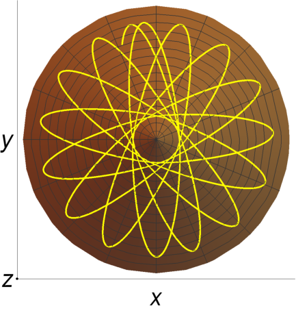
Below we shall see that when $\alpha=\nu^{2}$, the projection to the plane orthogonal to $\boldmathe{J}$ of the trajectory shown on the last plot is an ellipse centered at the origin of the coordinate system similarly to the case of the three-dimensional isotropic harmonic oscillator. This corresponds to a fundamental universal property of the magnetic monopole background which we discuss in the last section. Since the center of the projected elliptical trajectory is in the center of an ellipse, the angular period $P_{a}$ is twice the radial period $P_{r}$, $P_{a}/P_{r}=2$, similarly to the isotropic harmonic oscillator. This is different from the picture of the finite orbits in Kepler problem where the force center is in one of the foci, and as a result $P_{a}=P_{r}$. This similarity with the isotropic oscillator and contrast to the Kepler problem are also reflected in the spectra of the systems at the quantum level.

In this subsection we derive the conformal Newton-Hooke symmetry [61, 62, 63, 64] for the system (2.1) and compare it with the conformal symmetry of the model with $\omega=0$ studied in [32].

Using the AFF form of the Hamiltonian (2.8), one can show that the complex quantity

$$\,{\mathcal{C}}=e^{2i\omega t}\left(\frac{\pi_{r}^{2}}{2m}+\frac{\mathscr{L}^{2}}{2mr^{2}}-\frac{m\omega^{2}r^{2}}{2}-i\omega r\pi_{r}\right)=e^{2i\omega t}\left(H-m\omega^{2}r^{2}-i\omega r\pi_{r}\right)\,,$$

(2.22)

and its complex conjugate $\,{\mathcal{C}}^{*}$ are explicitly depending on time integrals of motion which together with $H$ generate the $\mathfrak{sl}(2,\mathbb{R})$ algebra

$$\{H,\,{\mathcal{C}}\}=2i\omega\,{\mathcal{C}}\,,\quad\{H,\,{\mathcal{C}}^{*}\}=-2i\omega\,{\mathcal{C}}^{*}\,,\quad\{\,{\mathcal{C}},\,{\mathcal{C}}^{*}\}=-4i\omega H\,.$$

(2.23)

In terms of $\,{\mathcal{C}}$ and $\,{\mathcal{C}}^{*}$, the generators of the Newton-Hooke symmetry are given by

$$D=\frac{i}{4\omega}(\,{\mathcal{C}}-\,{\mathcal{C}}^{*})\,,\qquad K=\frac{1}{4\omega^{2}}(2H-\,{\mathcal{C}}-\,{\mathcal{C}}^{*})\,,$$

(2.24)

and together with $H$ they satisfy the algebra

$$\{D,H\}=H-2\omega^{2}K\,,\qquad\{D,K\}=-K\,,\qquad\{K,H\}=2D\,,$$

(2.25)

whose Casimir invariant is

$$\mathscr{F}=D^{2}+\omega^{2}K^{2}-KH=-\frac{1}{4}\mathscr{L}^{2}\,.$$

(2.26)

In terms of these generators, the function $r^{2}(t)$ is presented in the form

$$r^{2}(t)=\frac{2}{m\omega^{2}}\big(\omega D\sin(2\omega t)+\omega^{2}K\cos(2\omega t)+H\sin^{2}(\omega t)\big)\,.$$

(2.27)

The values of the dynamical integrals $D$ and $K$ depend on the choice of initial conditions for $\boldmathe{r}$ and $\dot{\boldmathe{r}}$, and as follows from (2.22) and (2.24), our choice $r(0)=r_{\mathrm{min}}$, $\dot{r}(0)=0$ corresponds to $D=0$ and $K=\frac{1}{2}mr_{\mathrm{min}}^{2}$. For these values of $D$ and $K$, (2.27) takes the form (2.13). On the other hand, since $\boldmathe{J}\cdot\boldmathe{r}(t)=-\nu r(t)$, for a general choice of initial conditions Eq. (2.27) shows that the dynamics of the projection of $\boldmathe{r}(t)$ on the direction of the conserved angular momentum is controlled by the conformal Newton-Hooke symmetry of the system. According to (2.27), the oscillation period of $r(t)$ is $\pi/\omega$, and taking into account the value of the Casimir invariant, one can check that in the general case Eq. (2.27) also implies that $r(t)$ oscillates between the values $r_{\mathrm{min}}$ and $r_{\mathrm{max}}$ given by Eq. (2.11).

To conclude this part of the analysis, we comment on the limit $\omega\rightarrow 0$. In this case the generators $H$, $D$ and $K$ take the form

$$H_{0}=\frac{\pi_{r}^{2}}{2m}+\frac{\mathscr{L}^{2}}{2mr^{2}}\,,\qquad D_{0}=\frac{1}{2}r\pi_{r}-H_{0}t\,,\qquad K_{0}=\frac{mr^{2}}{2}-Dt-H_{0}t^{2}\,,$$

(2.28)

and satisfy the conformal algebra

$$\{D_{0},H_{0}\}=H_{0}\,,\qquad\{D_{0},K_{0}\}=-K_{0}\,,\qquad\{K_{0},H_{0}\}=2D_{0}\,.$$

(2.29)

The case $\alpha=0$ of the system $H_{0}$ corresponds to a geodesic motion on the dynamical cone [30, 31]. The special case of $\alpha=\nu^{2}$, on the other hand, was studied in [32]. It was shown there that the trajectory of the particle, projected to the plane orthogonal to $\boldmathe{J}$, is a straight line along which the projected particle’s motion takes place with constant velocity. Consistently with these peculiar properties, in the special case $\alpha=\nu^{2}$ the system with $H_{0}$ possesses a hidden symmetry described by the integral of motion $\boldmathe{V}=\textit{\mbox{\boldmath$\pi$}}\times\boldmathe{J}$ being a sort of Laplace-Runge-Lenz vector, in the plane orthogonal to which and parallel to $\boldmathe{J}$ the particle’s trajectory lies [32]. In Fig. 3 some plots of the trajectories are shown for the system (2.28).

In the case $\alpha=\nu^{2}$ the particle described by the Hamiltonian (2.1) admits additional integrals of motion responsible for the closed nature of the trajectories for arbitrary choice of initial conditions. The integrals are derived by an algebraic approach as in Fradkin’s construction for the isotropic three-dimensional harmonic oscillator [12].

Let us first consider arbitrary values of $\alpha$ assuming, as we indicated above, $J^{2}>\nu^{2}$. Our first step is to introduce the vector quantities

	$\displaystyle\boldmathe{I}_{1}$	$\displaystyle=\textit{\mbox{\boldmath$\pi$}}\crossproduct\boldmathe{J}\cos(\omega t)+\omega m\boldmathe{r}\crossproduct\boldmathe{J}\sin(\omega t)\,,$		(2.30)
	$\displaystyle\boldmathe{I}_{2}$	$\displaystyle=\textit{\mbox{\boldmath$\pi$}}\crossproduct\boldmathe{J}\sin(\omega t)-\omega m\boldmathe{r}\crossproduct\boldmathe{J}\cos(\omega t)\,.$		(2.31)

The time-dependence of these vectors in the plane orthogonal to $\boldmathe{J}$ follows from the time-dependence of $\pi$ and $\boldmathe{r}$ in (2.3),

$$\frac{d\boldmathe{I}_{1}}{dt}=\frac{1}{mr^{3}}(\alpha-\nu^{2})\boldmathe{n}\crossproduct\boldmathe{J}\cos(\omega t)\,,\qquad\frac{d\boldmathe{I}_{2}}{dt}=\frac{1}{mr^{3}}(\alpha-\nu^{2})\boldmathe{n}\crossproduct\boldmathe{J}\sin(\omega t)\,.$$

(2.32)

Then

$$\boldmathe{I}_{1}\cdot\boldmathe{I}_{2}=\frac{1}{2}(\nu^{2}-\alpha)(J^{2}-\nu^{2})\frac{\sin(2\omega t)}{2r^{2}}\,,$$

(2.33)

where we have taken into account our choice of the initial condition $\pi_{r}(0)=0$. The initial values of these vectors are

$$\boldmathe{I}_{1}(0)=\frac{J^{2}}{r_{\mathrm{min}}}\boldmathe{n}_{\bot}(0)\,,\qquad\boldmathe{I}_{2}(0)=m\omega r_{\mathrm{min}}\boldmathe{J}\crossproduct\boldmathe{n}_{\bot}(0)\,.$$

(2.34)

Thus, $\boldmathe{I}_{1}$ and $\boldmathe{I}_{2}$ are orthogonal to each other at $t=0$, but in general case of $\alpha\neq\nu^{2}$ their scalar product is not zero and changes periodically with period $\pi/\omega$.

For the particular choice $\alpha=\nu^{2}$, the vectors $\boldmathe{I}_{1}$ and $\boldmathe{I}_{2}$ are orthogonal vector integrals of motion of order 2 in the kinetic momenta, and so, they correspond to the “hidden symmetries” [1] of the system. They are, however, dynamical, explicitly time-dependent integrals of motion (similarly to generators of the conformal Newton-Hook symmetry $D$ and $K$), $\frac{d}{dt}\boldmathe{I}_{1,2}=\frac{\partial\boldmathe{I}_{1,2}}{\partial t}+\{\boldmathe{I}_{1,2},H\}=0$. Their lengths are also dynamical integrals whose values, again in the sense of a total time derivative, take constant values

$$|\boldmathe{I}_{1}|=m\omega\sqrt{J^{2}-\nu^{2}}\,r_{\mathrm{max}},\qquad|\boldmathe{I}_{2}|=m\omega\sqrt{J^{2}-\nu^{2}}\,r_{\mathrm{min}}\,,$$

(2.35)

where we have taken into account Eqs. (2.34) and (2.12). The sum of their squares, however, is a true integral of motion whose value is a function of $H$ and $J$,

$$\boldmathe{I}_{1}^{2}+\boldmathe{I}_{2}^{2}=2mH(J^{2}-\nu^{2})\,.$$

(2.36)

These vectors point in the direction of the semi-axes of the elliptic trajectory in the plane orthogonal to $\boldmathe{J}$. The lengths of semi-major and semi-minor axes correspond to those of the vectors $r\boldmathe{n}_{\bot}(0)$ and $r\,\hat{\hskip-2.84526pt\boldmathe{J}}\crossproduct\boldmathe{n}_{\bot}(0)$, and are equal to $r_{\mathrm{max}}\sqrt{1-\nu^{2}/J^{2}},$ and $r_{\mathrm{min}}\sqrt{1-\nu^{2}/J^{2}}$. We note that in general case $\alpha\neq\nu^{2}$ the periodic change of the scalar product of $\boldmathe{I}_{1}$ and $\boldmathe{I}_{2}$ implies a precession of the orbit, see Fig. 2.

Let us now investigate in more detail the most interesting case $\alpha=\nu^{2}$ given by the Hamiltonian

$$H=\frac{\textit{\mbox{\boldmath$\pi$}}^{2}}{2m}+\frac{m\omega^{2}}{2}r^{2}+\frac{\nu^{2}}{2mr^{2}}\,.$$

(2.37)

To express the general solution in terms of the conserved $\boldmathe{J}$ and dynamical integrals $\boldmathe{I}_{1}$ and $\boldmathe{I}_{2}$ in (2.30) and (2.31), which for $\alpha=\nu^{2}$ become true integrals of motion, we note that

$\displaystyle\boldmathe{r}(t)\crossproduct\boldmathe{J}=\frac{1}{m\omega}(\boldmathe{I}_{1}\sin(\omega t)-\boldmathe{I}_{2}\cos(\omega t))\,,\qquad\textit{\mbox{\boldmath$\pi$}}(t)\crossproduct\boldmathe{J}=\boldmathe{I}_{1}\cos(\omega t)+\boldmathe{I}_{2}\sin(\omega t)\,.$

(2.38)

By means of the relations

$$\boldmathe{J}\crossproduct(\boldmathe{r}(t)\crossproduct\boldmathe{J})=J^{2}\boldmathe{r}(t)+\nu r(t)\boldmathe{J}\,,\qquad|\boldmathe{r}\crossproduct\boldmathe{J}|^{2}=(J^{2}-\nu^{2})r^{2}(t)\,,\qquad$$

(2.39)

we can express the position $\boldmathe{r}(t)$ of the particle as follows,

$$\boldmathe{r}(t)=\frac{1}{m\omega J^{2}}\left(\boldmathe{J}\crossproduct\boldmathe{I}_{1}\sin\omega t-\boldmathe{J}\times\boldmathe{I}_{2}\cos\omega t-\nu\frac{\sqrt{I_{1}^{2}\sin^{2}\omega t+I_{2}^{2}\cos^{2}\omega t}}{\sqrt{J^{2}-\nu^{2}}}\boldmathe{J}\right)\,,$$

(2.40)

with $\boldmathe{I}_{1}=\boldmathe{I}_{1}(0)$ and $\boldmathe{I}_{2}=\boldmathe{I}_{2}(0)$. This yields us $\boldmathe{r}(t)$ and kinetic momentum $\textit{\mbox{\boldmath$\pi$}}=m\dot{\boldmathe{r}}$ at any given time presented in terms of the angular momentum and dynamical vector integrals.

Alternatively, one can follow a more algebraic approach to extract information on the trajectories without explicitly solving the equations of motion. It is well known from the seminal paper of Fradkin [12] that for the three-dimensional isotropic harmonic oscillator all symmetries of the trajectories are encoded in a tensor integral of motion. In the remainder of this subsection we construct an analogous tensor for the system at hand to find the trajectories by a linear algebra techniques. We begin with the tensor integrals

$$T^{ij}=T^{(ij)}+T^{[ij]}\,,\qquad T^{(ij)}=\frac{1}{2}(I_{1}^{i}I_{1}^{j}+I_{2}^{i}I_{2}^{j})\,,\qquad T^{[ij]}=\frac{1}{2}(I_{1}^{i}I_{2}^{j}-I_{1}^{j}I_{2}^{i})\,.$$

(2.41)

They, unlike the vectors $\boldmathe{I}_{1}$ and $\boldmathe{I}_{2}$, but like the quadratic expression (2.36) are the true, not depending explicitly on time integrals of motion, $\frac{d}{dt}T^{ij}=\{T^{ij},H\}=0$, whose explicit form in phase space variables is

$$2T^{ij}=(\textit{\mbox{\boldmath$\pi$}}\times\boldmathe{J})^{i}(\textit{\mbox{\boldmath$\pi$}}\times\boldmathe{J})^{j}+m^{2}\omega^{2}(\boldmathe{r}\times\boldmathe{J})^{i}(\boldmathe{r}\times\boldmathe{J})^{j}+\epsilon^{ijk}m\omega(J^{2}-\nu^{2})J_{k}\,.$$

(2.42)

In accordance with (2.36), their components satisfy relations

$$\text{tr}(T)=m(J^{2}-\nu^{2})H\,,\qquad\epsilon_{ijk}T^{[jk]}=m\omega(J^{2}-\nu^{2})J_{i}\,.$$

(2.43)

As the anti-symmetric part of $T^{ij}$ is related with the Poincaré integral, we only need to use the symmetric part $T^{(ij)}$, which is related but not identical to Fradkin’s tensor. Since the vectors (2.30), (2.31) are orthogonal to each other and to $\boldmathe{J}$, we immediately conclude that $\boldmathe{J},\boldmathe{I}_{1}$ and $\boldmathe{I}_{2}$ are eigenvectors of $T^{(ij)}$ with eigenvalues equal, respectively, to zero and

	$\displaystyle\lambda_{1}=|\boldmathe{I}_{1}|^{2}$	$\displaystyle=\frac{1}{2}m^{2}\omega^{2}(J^{2}-\nu^{2})r^{2}_{\mathrm{max}}\,,$		(2.44)
	$\displaystyle\lambda_{2}=|\boldmathe{I}_{2}|^{2}$	$\displaystyle=\frac{1}{2}m^{2}\omega^{2}(J^{2}-\nu^{2})r^{2}_{\mathrm{min}}\,,$		(2.45)

where we have taken into account (2.35). The relations

$$\boldmathe{I}_{1}\cdot\boldmathe{r}=(J^{2}-\nu^{2})\cos(\omega t)\,,\qquad\boldmathe{I}_{2}\cdot\boldmathe{r}=(J^{2}-\nu^{2})\sin(\omega t)\,,$$

(2.46)

allow us to conclude that the quadratic form $\boldmathe{r}^{T}T\boldmathe{r}$ is time-independent,

$$2r_{i}T^{ij}r_{j}=(\boldmathe{I}_{1}\cdot\boldmathe{r})^{2}+(\boldmathe{I}_{2}\cdot\boldmathe{r})^{2}=(J^{2}-\nu^{2})^{2}\,.$$

(2.47)

In a coordinate system with orthonormal base $\boldmathe{e}_{x}=\hat{\boldmathe{I}}_{1},\boldmathe{e}_{y}=\hat{\boldmathe{I}}_{2}$ and $\boldmathe{e}_{z}=\hat{\boldmathe{J}}$, the quadratic form (2.47) simplifies to

$$\lambda_{1}x^{2}+\lambda_{2}y^{2}=(J^{2}-\nu^{2})^{2}\,.$$

(2.48)

With $r_{\mathrm{max}}r_{\mathrm{min}}=J/(m\omega)$ one ends up with the equation for an ellipse in the plane orthogonal to $\boldmathe{J}$:

$$\frac{x^{2}}{r^{2}_{\mathrm{min}}}+\frac{y^{2}}{r^{2}_{\mathrm{max}}}=\frac{J^{2}-\nu^{2}}{J^{2}}\,.$$

(2.49)

The lengths of the semi-major axis and semi-minor axis of the ellipse are $r_{\mathrm{max}}\sqrt{1-\nu^{2}/J^{2}}$, $r_{\mathrm{min}}\sqrt{1-\nu^{2}/J^{2}}$ in accordance with that was found above.

For quantum theory it is of advantage to use the complex form of dynamical integrals of motion

$$\boldmathe{a}=\frac{1}{\sqrt{2}}(\boldmathe{I}_{1}+i\boldmathe{I}_{2})=\boldmathe{b}\crossproduct\boldmathe{J}\,e^{i\omega t}\,,\quad\boldmathe{b}=\frac{1}{\sqrt{2}}(\textit{\mbox{\boldmath$\pi$}}-i\omega m\boldmathe{r})\,,$$

(2.50)

and its complex conjugate $\boldmathe{a}^{*}$. They satisfy the non-linear Poisson bracket relations

	$\displaystyle\{H,\boldmathe{a}\}=i\omega\boldmathe{a}\,,\qquad\{J_{i},a_{j}^{\#}\}=\epsilon_{ijk}a_{k}^{\#}\,,\qquad\{a_{i}^{\#},a_{j}^{\#}\}=-m\,\,{\mathcal{C}}^{\#}\epsilon_{ijk}J_{k}\,,$		(2.51)
	$\displaystyle\{a_{i}^{*},a_{j}\}=im\omega[(2J^{2}-\nu^{2})\delta_{ij}-J_{i}J_{j})]-mH\epsilon_{ijk}J_{k}\,,$		(2.52)

and are related to the generators (2.22) of the conformal symmetry,

$\displaystyle a_{i}^{\#}a_{i}^{\#}=m(J^{2}-\nu^{2})\,{\mathcal{C}}^{\#}\,,$

(2.53)

where $a^{\#}_{i}$ denotes either $a_{i}$ or $a^{*}_{i}$, and similarly for $\,{\mathcal{C}}$, $\,{\mathcal{C}}^{*}$. The $a^{\#}_{i}$ and $\,{\mathcal{C}}^{\#}$ are classical analogues of the ladder operators in the related quantum system. In terms of $a^{\#}_{i}$ the tensor integrals $T_{(ij)}=T^{(ij)}$ and $T_{[ij]}=T^{[ij]}$ take the form

$$T_{(ij)}=\tfrac{1}{2}\big(a_{i}^{*}a_{j}+a_{j}^{*}a_{i}\big),\qquad T_{[ij]}=\tfrac{i}{2}\big(a_{i}a_{j}^{*}-a_{j}a_{i}^{*}\big)=\tfrac{1}{2}m\omega(J^{2}-\nu^{2})\epsilon_{ijk}J_{k}\,.$$

(2.54)

In fact, such kind of tensors were considered in earlier studies of the quantized system by Vinet et al [65]. We find it useful to exploit these integrals for the classical system at hand.

Symmetric tensor integral $T_{(ij)}$ satisfies the Poisson bracket reations

$$\{J_{i},T_{(jk)}\}=\epsilon_{ijl}T_{(lk)}+\epsilon_{ikl}T_{(jl)}\,,$$

(2.55)

and

$$\{T_{(ij)},T_{(lk)}\}=m(\epsilon_{ils}\mathcal{F}_{jk}+\epsilon_{iks}\mathcal{F}_{jl}+\epsilon_{jls}\mathcal{F}_{ik}+\epsilon_{jks}\mathcal{F}_{im})J_{s}\,,$$

(2.56)

where

$$\mathcal{F}_{ij}=\tfrac{1}{4}m\omega^{2}(J^{2}-\nu^{2})^{2}\delta_{ij}-HT_{(ij)}\,,$$

(2.57)

and we have used Eqs. (2.51), (2.52) and the equality

$$\,{\mathcal{C}}^{*}a_{i}a_{j}+a_{i}^{*}a_{j}^{*}\,{\mathcal{C}}=2HT_{(ij)}+m\omega^{2}(J^{2}-\nu^{2})[J^{2}\delta_{ij}-J_{i}J_{j}]\,.$$

(2.58)

In the following section we shall see that the quantum analog of the classical integrals of motion $\,{\mathcal{C}}^{\#}$ and $\boldmathe{a}^{\#}$, due to their dynamical nature of conservation, provide us with a complete set of the spectrum generating operators for the quantum system with Hamiltonian (2.37).

To conclude this section, we comment on the limit $\nu\rightarrow 0$, when we recover the isotropic harmonic oscillator. In this limit the integral $\boldmathe{a}$ and its complex conjugate reduce to the vector product of the orbital angular momentum and the classical analogs of the first order ladder operators. Instead of considering the dynamical integral $\boldmathe{a}$ one may choose the vector

$$\boldmathe{z}=\big(\boldmathe{b}+\frac{\nu}{J^{2}}(\boldmathe{b}\cdot\boldmathe{n})\boldmathe{J}\big)e^{i\omega t}=\frac{1}{J^{2}}\boldmathe{J}\crossproduct\boldmathe{a}\,$$

(2.59)

with $\boldmathe{b}$ defined in (2.50). This integral and its complex conjugate, which indeed contain the same physical information as $\boldmathe{a}$ and $\boldmathe{a}^{\#}$, fulfill the Poisson bracket relations

$$\{\boldmathe{z}_{i}^{\#},\boldmathe{z}_{k}^{\#}\}=-\frac{\nu^{2}}{2J^{4}}\,{\mathcal{C}}^{\#}\epsilon_{ikl}J_{l}\,,\qquad\{\boldmathe{z}_{i},\boldmathe{z}_{k}^{*}\}=-im\omega\delta_{i,k}+\frac{1}{J^{4}}\mathcal{O}(\nu^{2})\,,$$

(2.60)

where $\mathcal{O}(\nu^{2})$ are terms of order $\nu^{2}$. In the limit $\nu\rightarrow 0$ they are just the classical analogs of the first order ladder operators satisfying the Heisenberg algebra. However, the appearance of the non-local operator $1/J^{2}$ in quantum mechanics complicates the analysis considerably and we prefer to use the integrals (2.50) to deal with local operators in what follows.

References

- [1] M. Cariglia, “Hidden symmetries of dynamics in classical and quantum physics,” Rev. Mod. Phys. 86, 1283 (2014) [arXiv:1411.1262[math-th]].
- [2] O. Evnin and R. Nivesvivat, “Hidden symmetries of the Higgs oscillator and the conformal algebra,” J. Phys. A 50 no.1, 015202 (2017) [arXiv:1604.00521 [nlin.SI]].
- [3] O. Evnin and C. Krishnan, “A hidden symmetry of AdS resonances,” Phys. Rev. D 91, 126010 (2015) [arXiv:1502.03749 [hep-th]].
- [4] O. Evnin and R. Nivesvivat, “AdS perturbations, isometries, selection rules and the Higgs oscillator,” JHEP 1601, 151 (2016) [arXiv:1512.00349 [hep-th]].
- [5] S. P. Novikov, S.V. Manakov, L. P. Pitaevskii, and V. E. Zakharov, Theory of Solitons (Plenum, New York, 1984).
- [6] F. Correa, O. Lechtenfeld and M. Plyushchay, “Nonlinear supersymmetry in the quantum Calogero model,” JHEP 1404, 151 (2014) [arXiv:1312.5749 [hep-th]].
- [7] V. Frolov, P. Krtous and D. Kubiznak, “Black holes, hidden symmetries, and complete integrability,” Living Rev. Rel. 20, no. 1, 6 (2017) [arXiv:1705.05482 [gr-qc]].
- [8] A. Kirchberg, J. D. Lange, P. A. G. Pisani and A. Wipf, “Algebraic solution of the supersymmetric hydrogen atom in d-dimensions,” Annals Phys. 303, 359 (2003), [hep-th/0208228].
- [9] E. Ivanov, S. Krivonos and O. Lechtenfeld, “New variant of N=4 superconformal mechanics,” JHEP 0303, 014 (2003) [hep-th/0212303].
- [10] F. Correa, V. Jakubsky, L. M. Nieto and M. S. Plyushchay, “Self-isospectrality, special supersymmetry, and their effect on the band structure,” Phys. Rev. Lett. 101, 030403 (2008) [arXiv:0801.1671 [hep-th]].
- [11] M. S. Plyushchay, “Nonlinear supersymmetry as a hidden symmetry,” In: Integrability, Supersymmetry and Coherent States. Ş. Kuru, J. Negro and L.M. Nieto (eds). CRM Series in Mathematical Physics. Springer, Cham (2019) 163-186 [arXiv:1811.11942 [hep-th]].
- [12] D. M. Fradkin, “Three-dimensional isotropic harmonic oscillator and SU3,” Am. J. Phys. 33, 207 (1965).
- [13] W. Pauli, “Über das Wasserstoffspektrum vom Standpunkt der neuen Quantenmechanik,” Z. Physik 36, 336 (1926).
- [14] D. Zwanziger, “Exactly soluble nonrelativistic model of particles with both electric and magnetic charges,” Phys. Rev. 176, 1480 (1986).
- [15] A. Arancibia and M. S. Plyushchay, ““Chiral asymmetry in propagation of soliton defects in crystalline backgrounds,” Phys. Rev. D 92, no. 10, 105009 (2015) [arXiv:1507.07060 [hep-th]].
- [16] J. F. Cariñena and M. S. Plyushchay, “ABC of ladder operators for rationally extended quantum harmonic oscillator systems,” J. Phys. A 50 (2017) no.27, 275202 [arXiv:1701.08657 [math-ph]].
- [17] J. Mateos Guilarte and M. S. Plyushchay, “Perfectly invisible PT-symmetric zero-gap systems, conformal field theoretical kinks, and exotic nonlinear supersymmetry,” JHEP 1712, 061 (2017) [arXiv:1710.00356 [hep-th]].
- [18] J. Mateos Guilarte and M. S. Plyushchay, “Nonlinear symmetries of perfectly invisible PT-regularized conformal and superconformal mechanics systems,” JHEP 1901, 194 (2019) [arXiv:1806.08740[hep-th]].
- [19] J. F. Cariñena, L. Inzunza and M. S. Plyushchay, “Rational deformations of conformal mechanics”, Phys. Rev. D 98, 026017 (2018) [arXiv:1707.07357 [math-ph]].
- [20] L. Inzunza and M. S. Plyushchay, “Hidden symmetries of rationally deformed superconformal mechanics”, Phys. Rev. D 99, no. 2, 025001 (2019) [arXiv:1809.08527 [hep-th]].
- [21] J. de Boer, F. Harmsze and T. Tjin, “Nonlinear finite W symmetries and applications in elementary systems,” Phys. Rept. 272, 139 (1996) [arXiv:hep-th/9503161].
- [22] E. D’Hoker and L. Vinet, “Supersymmetry of the Pauli equation in the presence of a magnetic monopole,” Phys. Lett. 137B, 72 (1984).
- [23] E. D’Hoker and L. Vinet, “Dynamical supersymmetry of the magnetic monopole and the potential,” Commun. Math. Phys. 97, 391 (1985).
- [24] F. De Jonghe, A. J. Macfarlane, K. Peeters, J. W. van Holten, “New supersymmetry of the monopole,” Phys. Lett. B 359, 114 (1995) [arXiv:hep-th/9507046].
- [25] G. W. Gibbons, R. H. Rietdijk and J. W. van Holten, “SUSY in the sky,” Nucl. Phys. B 404, 42 (1993) [arXiv:hep-th:9303112].
- [26] M. Tanimoto, “The role of Killing-Yano tensors in supersymmetric mechanics on a curved manifold,” Nucl. Phys. B 442, 549 (1995) [arXiv:gr-qc/9501006].
- [27] M. Cariglia, “Quantum mechanics of Yano tensors: Dirac equation in curved spacetime,” Class. Quant. Grav. 21, 1051 (2004) [arXiv:hep-th:0305153].
- [28] M. S. Plyushchay, “On the nature of fermion monopole supersymmetry,” Phys. Lett. B 485, 187 (2000) [arXiv:hep-th:0005122].
- [29] P. Goddard and D. I. Olive, “Magnetic monopoles in gauge field theories,” Rept. Prog. Phys. 41, 1357 (1978).
- [30] M. S. Plyushchay, “Monopole Chern-Simons term: Charge monopole system as a particle with spin,” Nucl. Phys. B 589, 413 (2000) [hep-th/0004032].
- [31] M. S. Plyushchay, “Free conical dynamics: Charge-monopole as a particle with spin, anyon and nonlinear fermion-monopole supersymmetry,” Nucl. Phys. Proc. Suppl. 102, 248 (2001) [hep-th/0103040].
- [32] M. S. Plyushchay and A. Wipf, “Particle in a self-dual dyon background: hidden free nature, and exotic superconformal symmetry,” Phys. Rev. D 89, no. 4, 045017 (2014) [arXiv:1311.2195 [hep-th]].
- [33] P. A. M. Dirac, “Forms of relativistic dynamics”, Rev. Mod. Phys. 21, 392 (1949).
- [34] L. Inzunza, M. S. Plyushchay and A. Wipf, “Conformal bridge between freedom and confinement,” [arXiv:1912.11752 [hep-th]].
- [35] E. Witten, “Dynamical breaking of supersymmetry,” Nucl. Phys. B 188, 513 (1981).
- [36] E. Witten, “Constraints on supersymmetry breaking,” Nucl. Phys. B 202, 253 (1982).
- [37] V. B. Matveev and M. A. Salle, Darboux Transformations and Solitons (Springer, Berlin, 1991).
- [38] F. Cooper, A. Khare and U. Sukhatme, “Supersymmetry and quantum mechanics,” Phys. Rept. 251, 267 (1995) [arXiv:hep-th/9405029].
- [39] A. Kirchberg, J. D. Lange and A. Wipf, “Extended supersymmetries and the Dirac operator,” Annals Phys. 315, 467 (2005) [hep-th/0401134].
- [40] S. Bellucci, S. Krivonos and A. Nersessian, “N=8 supersymmetric mechanics on special Kahler manifolds,” Phys. Lett. B 605, 181 (2005) [hep-th/0410029].
- [41] S. Bellucci, A. Nersessian and A. Yeranyan, “Hamiltonian reduction and supersymmetric mechanics with Dirac monopole,” Phys. Rev. D 74, 065022 (2006) [arXiv:hep-th:0606152].
- [42] N. Kozyrev, S. Krivonos, O. Lechtenfeld, A. Nersessian and A. Sutulin, “Curved Witten-Dijkgraaf-Verlinde-Verlinde equation and mechanics,” Phys. Rev. D 96, no. 10, 101702 (2017) [arXiv:1710.00884 [hep-th]].
- [43] N. Kozyrev, S. Krivonos, O. Lechtenfeld, A. Nersessian and A. Sutulin, “ supersymmetric mechanics on curved spaces,” Phys. Rev. D 97, no. 8, 085015 (2018) [arXiv:1711.08734 [hep-th]].
- [44] V. de Alfaro, S. Fubini and G. Furlan, “Conformal invariance in quantum mechanics,” Nuovo Cim. A 34, 569 (1976).
- [45] S. Fubini and E. Rabinovici, “Superconformal quantum mechanics,” Nucl. Phys. B 245, 17 (1984).
- [46] S. Fedoruk, E. Ivanov and O. Lechtenfeld, “Superconformal mechanics,” J. Phys. A, 45, 17 (2012) [arXiv:1112.1947[hep-th]].
- [47] R. Britto-Pacumio, J. Michelson, A. Strominger and A. Volovich, “Lectures on superconformal quantum mechaics and multi-black hole moduli spaces,” NATO Sci. Ser. C 556, 255 (2000) [arXiv:hep-th/9911066].
- [48] P. Claus, M. Derix, R. Kallosh, J. Kumar, P. K. Townsend and A. Van Proeyen, “Black holes and superconformal mechanics,” Phys. Rev. Lett. 81, 4553 (1998) [arXiv:hep-th/9804177].
- [49] J. A. de Azcárraga, J. M. Izquierdo, J. C. Pérez Bueno and P. K. Townsend, “Superconformal mechanics, black holes, and nonlinear realizations”, Phys. Rev. D 59, 084015 (1999) [arXiv:hep-th/9810230].
- [50] G. W. Gibbons and P. K. Townsend, “Black holes and Calogero models,” Phys. Lett. B 454, 187 (1999) [arXiv:hep-th/9812034].
- [51] J. Michelson and A. Strominger, “Superconformal multi-black hole quantum mechanics,” JHEP 9909, 005 (1999) [arXiv:hep-th/9908044].
- [52] C. Chamon, R. Jackiw, S. Y. Pi and L. Santos, “Conformal quantum mechanics as the CFT1 dual to AdS2,” Phys. Lett. B 701, 503 (2011) arXiv:106.0726 [hep-th]].
- [53] B. Pioline and A. Waldron, “Quantum Cosmology and Conformal Invariance,” Phys. Rev. Lett. 90, 031302 (2003) arXiv:0209044 [hep-th]].
- [54] J. B. Achour and E. R. Livine, “Cosmology as a CFT1,” JHEP 1912, 031 (2019) [arXiv:1909.13390 [gr-qc]]
- [55] S. Brodsky, G. de Teramond, H. Gunter and J. Erlich, “Light-front holographic QCD and emerging confinement”, Phys. Rept. 584, 1 (2015) [arXiv:1407.8131 [hep-ph]].
- [56] A. B. Balantekin, “Accidental degeneracies and supersymmetric quantum mechanics,” Ann. Phys. (NY) 164, 277 (1985).
- [57] M. Moshinsky and A. Szczepaniak, “The Dirac oscillator,” Journ. Phys. A: Mathematical and General 22, 17, L817 (1989).
- [58] J. Bentez, R. P. Martnez y Romero, H. N. Núez-Yépez, and A. L. Salas-Brito “Solution and hidden supersymmetry of a Dirac oscillator,” Phys. Rev. Lett. 64, 1643 (1990).
- [59] C. Quesne and M. Moshinsky, “Symmetry Lie algebra of the Dirac oscillator,” Journ. Phys. A: Mathematical and General 23, 12, 2263 (1990).
- [60] C. Quesne, “Supersymmetry and the Dirac oscillator,” Intern. Journ. Mod. Phys. A 06, 09, 1567 (1991).
- [61] U. Niederer, “The maximal kinematical invariance group of the harmonic oscillator,” Helv. Phys. Acta 46, 191 (1973).
- [62] A. Galajinsky, “Conformal mechanics in Newton-Hooke spacetime,” Nucl. Phys. B 832, 586 (2010) [arXiv:1002.2290 [hep-th]].
- [63] K. Andrzejewski, “Conformal Newton-Hooke algebras, Niederer’s transformation and Pais-Uhlenbeck oscillator,” Phys. Lett. B 738, 405 (2014) [arXiv:1409.3926 [hep-th]].
- [64] A. Galajinsky, “Geometry of the isotropic oscillator driven by the conformal mode,” Eur. Phys. J. C 78, no. 1, 72 (2018) [arXiv:1712.00742 [hep-th]].
- [65] S. Labelle, M. Mayrand, L. Vinet “Symmetries and degeneracies of a charged oscillator in the field of a magnetic monopole,” J. Math. Phys. 32, 1516 (1991).
- [66] H. V. Mcintosh and A. Cisneros, “Degeneracy in the presence of a magnetic monopole,” J. Math. Phys. 11 (1970) 896.
- [67] T. T. Wu and C. N. Yang, “Dirac monopole without strings: monopole harmonics,” Nucl. Phys. B 107, 365 (1976).
- [68] T. T. Wu and C. N. Yang, “Some properties of monopole harmonics,” Phys. Rev. D 16, 1018 (1977).
- [69] G. Lochak, “Wave equation for a magnetic monopole,” Int. J. Theor. Phys. (1985) 24: 1019.
- [70] M. S. Plyushchay, “Quantization of the classical system and representations of group,” J. Math. Phys. 34, 3954 (1993).
- [71] L. Inzunza and M. S. Plyushchay, “Klein four-group and Darboux duality in conformal mechanics,” Phys. Rev. D 99, 125016 (2019) [arXiv:1902.00538 [hep-th]].
- [72] A. Perelomov, Generelized Coherent States and Their Applications (Springer-Verlag, Berlin, 1986).
- [73] L. Inzunza and M. S. Plyushchay, “Hidden superconformal symmetry: Where does it come from?,” Phys. Rev. 97, 045002 (2018) [arXiv:1711.00616 [hep-th]].
- [74] L. D. Landau and E. M. Lifshitz, Quantum Mechaics. Course of Theoretical Physics, Vol. 3 (Pergamon Press, 1965).
- [75] H. Falomir, P. A. G. Pisani and A. Wipf, “Pole structure of the Hamiltonian zeta function for a singular potential,” J. Phys. A 35, 5427 (2002) [arXiv:math-ph/0112019].
- [76] H. Falomir and P. A. G. Pisani, “Self-adjoint extensions and SUSY breaking in supersymmetric quantum mechanics,” J. Phys. A 38, 4665 (2005) [arXiv:hep-th/0501083].
- [77] K. Kirsten and P. Loya, “Spectral functions for the Schrödinger operator on with a singular potential,” J. Math. Phys. 51, 053512 (2010).
- [78] A. Nersessian, “Elements of (super-)Hamiltonian formalism,” Lect. Notes Phys. 698, 139 (2006) [arXiv:hep-th:0506170].
- [79] L. Mardoyan, A. Nersessian and A. Yeranyan, “Relationship between quantum-mechanical systems with and without monopoles,” Phys. Lett. A 366, 30 (2007) [arXiv:hep-th:0610301].
- [80] M. Barriola and A. Vilenkin, “Gravitational field of a global monopole,” Phys. Rev. Lett. 63, 341 (1989).
- [81] A. Galajinsky and O. Lechtenfeld, “Spinning extensions of superconformal mechanics,” J. High Energ. Phys. 2019, 069 (2019) [arXiv:1902.06851 [hep-th]].
- [82] M. Cariglia, A. Galajinsky, G. W. Gibbons and P. A. Horvathy, “Cosmological aspects of the Eisenhart-Duval lift,” Eur. Phys. J. C 78, no. 4, 314 (2018) [arXiv:1802.03370 [gr-qc]].
- [83] J. Gamboa and M. Plyushchay, “Classical anomalies for spinning particles,” Nucl. Phys. B 512, 485 (1998) [arXiv:hep-th:9711170].
- [84] C. Leiva and M. S. Plyushchay, “Superconformal mechanics and nonlinear supersymmetry,” JHEP 0310, 069 (2003) [arXiv:hep-th:0304257].
- [85] A. Anabalon and M. S. Plyushchay, “Interaction via reduction and nonlinear superconformal symmetry,” Phys. Lett. B 572, 202 (2003) [arXiv:hep-th:0306210].
- [86] L. C. Biedenharn, J. D. Louck and P. A. Carruthers, Angular momentum in quantum physics: theory and application (Oxford University Press, Oxford 2009).