Task-Based Quantization with Application to MIMO ReceiversThis work received funding from the Benoziyo Endowment Fund for the Advancement of Science, the Estate of Olga Klein – Astrachan, the European Union’s Horizon 2020 research and innovation program under grant No. 646804-ERC-COG-BNYQ, and the Israel Science Foundation under grant No. 0100101. N. Shlezinger and Y. C. Eldar are with the Faculty of Math and CS, Weizmann Institute of Science, Rehovot, Israel (e-mail: nirshlezinger1@gmail.com; yonina@weizmann.ac.il).

We begin by briefly reviewing the standard quantization setup, and recall the definition of a quantizer:

In the standard quantization problem, a $Q_{M}^{n,n}\left(\cdot\right)$ quantizer is designed to minimize some distortion measure $d:\mathcal{X}^{n}\times\hat{\mathcal{X}}^{n}\mapsto\mathcal{R}^{+}$ between its input and its output. The performance of a quantizer is characterized using its quantization rate $R\triangleq\frac{1}{n}\log M$, and the expected distortion $\mathbb{E}\{d\left({{\boldsymbol{x}}},\hat{{{\boldsymbol{x}}}}\right)\}$. For a fixed input size $n$ and codebook size $M$, the optimal quantizer is $Q_{M}^{n,{\rm opt}}\left(\cdot\right)=\mathop{\arg\min}_{Q_{M}^{n,n}}\mathbb{E}\left\{d\left({{\boldsymbol{x}}},Q_{M}^{n,n}\left({{{\boldsymbol{x}}}}\right)\right)\right\}$. Characterizing the optimal quantizer and its trade-off between distortion and quantization rate is in general a very difficult task. Optimal quantizers are thus typically studied assuming either high quantization rate, i.e., $R\rightarrow\infty$, see, e.g., [24], or asymptotically large inputs, namely, $n\rightarrow\infty$, via rate-distortion theory [25, Ch. 10].

Here, we study task-based quantization [12], where the design objective of the quantizer is some task other than minimizing the distortion between its input and output. In the following, we focus on the generic task of acquiring a random vector ${{\boldsymbol{s}}}\in\mathcal{S}^{k}\subseteq\mathcal{R}^{k}$ from a statistically dependent random vector ${{\boldsymbol{x}}}\in\mathcal{R}^{n}$ of larger dimensionality, i.e., $n\geq k$. The set $\mathcal{S}$ represents the possible values of the unknown vector: It can be continuous, representing an estimation task; or discrete, for classification tasks. This formulation accommodates a broad range of applications, including channel estimation and symbol detection, that are the common tasks considered in mimo communications receivers [13], as well as covariance recovery [17], doa estimation [18], and source localization [26]. The recovered estimate of ${{\boldsymbol{s}}}$, denoted $\hat{{{\boldsymbol{s}}}}$, is represented in digital using up to $\log M$ bits, dictating the bit budget allowed for task-based quantization. The observed ${{\boldsymbol{x}}}$ is related to ${{\boldsymbol{s}}}$ via a conditional probability measure $f_{{{\boldsymbol{x}}}|{{\boldsymbol{s}}}}$. For example, in a communications setup. the conditional probability measure $f_{{{\boldsymbol{x}}}|{{\boldsymbol{s}}}}$ encapsulates the noisy channel.

The performance limits of task-based quantization with asymptotically large vectors, i.e., when $n\rightarrow\infty$ while $R=\frac{1}{n}\log M$ remains fixed, can be characterized using indirect rate-distortion theory [27]. Specifically, for estimation tasks with the mse distortion objective, i.e., $d({\boldsymbol{s}},\hat{{\boldsymbol{s}}})=\|{\boldsymbol{s}}-\hat{{\boldsymbol{s}}}\|^{2}$, the task-based quantization mapping which minimizes the mse for a fixed quantization rate $R$ was derived in [28] for fixed-size vectors. The resulting optimal strategy consists of applying vector quantization to the mmse (mmse) estimate of ${\boldsymbol{s}}$ from ${\boldsymbol{x}}$.

While vector quantizers allow to achieve more accurate digital representations of the acquired analog signal compared to their scalar counterparts [29, Ch. 23], practical adc typically utilize scalar quantizers. In particular, adc often apply the same continuous-to-discrete mapping to each sample, which is most commonly based on a uniform partition of the real line, i.e., scalar uniform quantization [4]. Nonetheless, in the presence of a task, one is not interested in recovering the analog signal, but rather estimate some underlying information embedded in it. This motivates the analysis of how to incorporate the presence of a task in the design of a quantization system utilizing scalar adc, and whether the distortion induced by conventional scalar quantization can be mitigated when recovering the task.

As discussed in the previous section, practical digital signal processing systems typically obtain a discrete representation of physical analog signals using scalar adc. In such systems, each continuous-amplitude sample is converted into a discrete representation using a single quantization rule. Therefore, in order to be able to account for the presence of a task in acquisition while operating with scalar adc, one must introduce some level of processing, in addition to that carried out in digital. We therefore consider hybrid acquisition systems as illustrated in Fig. 2, which is a common model in mimo communication receivers [19, 20]. Hybrid architectures were originally proposed as a method to reduce the number of costly RF chains in mimo receivers [19, 20], while here we exploit these structures to allow quantization under bit constraints for tasks. In such hybrid systems, a set of analog signals can be combined in analog prior to being converted to digital, a property which we exploit in order to facilitate extracting some desired information from them. This model can represent, e.g., sensor arrays or mimo receivers, and specializes the case of a single analog input signal. While acquiring a set of analog signals in digital hardware includes both sampling, i.e., continuous-to-discrete time conversion, as well as quantization, we henceforth focus only the quantization aspect assuming a fixed sampling mechanism. The joint design of sampling and quantization in light of a task is left for future studies; initial results can be found in [30].

In the proposed hybrid architecture, the input to the adc, denoted ${{\boldsymbol{z}}}\in\mathcal{R}^{p}$, where $p$ denotes the number of scalar quantizers, is obtained from ${{\boldsymbol{x}}}$ using a pre-quantization mapping referred to as analog combining. Then, ${{\boldsymbol{z}}}$ is quantized using $p$ identical scalar quantizers with resolution $\tilde{M}\triangleq\lfloor M^{1/p}\rfloor$ into a digital vector $Q({{\boldsymbol{z}}})$. The overall number of bits is $p\cdot\log\tilde{M}\leq\log M$. The adc output is processed in digital to obtain the estimate $\hat{{{\boldsymbol{s}}}}\in\mathcal{S}^{k}$. A schematic block diagram of the quantization system is depicted in Fig. 3. Designing task-based quantizers can be formulated as the joint optimization of the analog combining mapping, the scalar quantization rule, and the digital processing, such that the output $\hat{{{\boldsymbol{s}}}}$ will be an accurate estimate of the task vector ${{\boldsymbol{s}}}$, while operating under a fixed budget of up to $\log M$ bits.

The characterization of task-based quantization systems of the form of Fig. 3 consists of two complementary studies: First, we study in Section III how the overall system can be designed based on knowledge of the conditional distribution $f_{{{\boldsymbol{x}}}|{{\boldsymbol{s}}}}$ relating the observations and the task in a model-based fashion. Then, we discuss how task-based quantization mappings can be learned from labeled data building upon ml tools, and in particular, by utilizing dnn to adapt task-based quantization mappings, in Section IV. Our results demonstrate that by properly tuning the hybrid architecture of task-based quantizers, one can approach the performance limits dictated by indirect rate-distortion theory, achievable using complex vector quantizers, while using conventional scalar adc operating as part of an acquisition system of feasible hardware requirements.

In order to obtain a meaningful and tractable characterization of the task-based quantization system of Fig. 3, we henceforth introduce two model assumptions upon which we base our results in the remainder of this section:

1. A1

   We consider the task of estimating the task ${{\boldsymbol{s}}}$ in the mse sense, namely, our performance measure is the mse $\mathbb{E}\{\|{{\boldsymbol{s}}}-\hat{{{\boldsymbol{s}}}}\|^{2}\}$.

2. A2

   We focus on uniform adc, and model the their operation in our derivations as non-subtractive uniform dithered quantizers [31].

Model assumption A1 implies that the fidelity of an estimate $\hat{{{\boldsymbol{s}}}}$ can be represented as a sum of the mmse and the excess mse with respect to the mmse estimate $\tilde{{{\boldsymbol{s}}}}=\mathbb{E}\{{{\boldsymbol{s}}}|{{\boldsymbol{x}}}\}$, as $\mathbb{E}\{\|{{\boldsymbol{s}}}-\hat{{{\boldsymbol{s}}}}\|^{2}\}=\mathbb{E}\{\|{{\boldsymbol{s}}}-\tilde{{{\boldsymbol{s}}}}\|^{2}\}+\mathbb{E}\{\|\tilde{{{\boldsymbol{s}}}}-\hat{{{\boldsymbol{s}}}}\|^{2}\}$. Consequently, in the following we characterize the performance in terms of the excess mse $\mathbb{E}\{\|\tilde{{{\boldsymbol{s}}}}-\hat{{{\boldsymbol{s}}}}\|^{2}\}$. Since $\tilde{{{\boldsymbol{s}}}}$ is a function of ${{\boldsymbol{x}}}$, we divide our analysis based on the nature of this function, considering linear functions in Section III-B, extending to quadratic and more general forms in Section III-C.

Model assumption A2 imposes a structure on the scalar quantization mapping. To formulate the resulting input-output relationship of the adc, let $\gamma$ denote the support of the quantizer, and define $\Delta\triangleq\frac{2\gamma}{\tilde{M}}$ as the quantization spacing. The output of the uniform adc with input sequence $z_{1},z_{2},\ldots,z_{p}$ can be written as $Q\left(z_{i}\right)=q\left(z_{i}+u_{i}\right)$, where $u_{1},u_{2},\ldots,u_{p}$ are i.i.d. rv uniformly distributed over $\left[-\frac{\Delta}{2},\frac{\Delta}{2}\right]$, mutually independent of the input, representing the dither signal. The function $q(\cdot)$, which implements the uniform quantization, is given by

When $\tilde{M}=2$, the resulting quantizer is a standard one-bit sign quantizer of the form $q(z)=c\cdot{\rm sign}(z)$, where $c>0$ is determined by the support $\gamma$.

Dithered quantizers significantly facilitate the analysis, due to the following favorable property: When operating within the support, the output can be written as the sum of the input and an additive zero-mean white quantization noise signal uncorrelated with the input. The drawback of adding dither is that it increases the energy of the quantization noise, namely, it results in increased distortion [31]. Nonetheless, the favorable property of dithered quantization is also satisfied in uniform quantization without dithering for inputs with bandlimited characteristic functions, and is approximately satisfied for various families of input distributions [32]. Consequently, while our analysis assumes dithered quantization, exploiting the resulting statistical properties of the quantization noise, the proposed system is applicable without dithering, as we demonstrate in our numerical study.

We begin by focusing on scenarios in which the stochastic relationship between the vector of interest ${{\boldsymbol{s}}}$ and the observations ${{\boldsymbol{x}}}$ are such that the mmse estimate of ${{\boldsymbol{s}}}$ from ${{\boldsymbol{x}}}$ is a linear function of ${{\boldsymbol{x}}}$, i.e., $\exists{\boldsymbol{\Gamma}}\in\mathcal{R}^{k\times n}$ such that $\tilde{{{\boldsymbol{s}}}}={\boldsymbol{\Gamma}}{{\boldsymbol{x}}}$. Accordingly, we restrict the analog combining and the digital mapping components in Fig. 3 to be linear, namely, ${{\boldsymbol{z}}}={\boldsymbol{A}}{{\boldsymbol{x}}}$ and $\hat{{{\boldsymbol{s}}}}={\boldsymbol{B}}Q({{\boldsymbol{z}}})$, for some ${\boldsymbol{A}}\in\mathcal{R}^{p\times n}$ and ${\boldsymbol{B}}\in\mathcal{R}^{k\times p}$. An illustration of the considered system architecture is depicted in Fig. 4.

By focusing on these setups, we are able to explicitly derive the achievable distortion and to characterize the system which minimizes the mse. This derivation reveals some non-trivial insights. For example, we show that the optimal approach when using vector quantizers, namely, to quantize the mmse estimate [28], is no longer optimal when using standard scalar adc. Furthermore, as detailed in Section III-C, our analysis provides guidelines for designing task-based quantization systems which can be used for more general relationships between ${{\boldsymbol{s}}}$ and ${{\boldsymbol{x}}}$, such as the recovery of quadratic tasks.

Let ${\boldsymbol{\Sigma}}_{{{\boldsymbol{x}}}}$ be the covariance matrix of ${{\boldsymbol{x}}}$, assumed to be non-singular. Before we study the overall task-based quantization system, we first derive the digital processing matrix which minimizes the mse for a given analog combiner ${\boldsymbol{A}}$ and the resulting mse, stated in the following lemma [12, Lem. 1]:

The digital processing matrix in Lemma 2 is the linear mmse estimator of ${{\boldsymbol{s}}}$ from the vector ${\boldsymbol{A}}{{\boldsymbol{x}}}+{\boldsymbol{e}}$, where ${\boldsymbol{e}}$ represents the quantization noise, which is white and uncorrelated with ${\boldsymbol{A}}{{\boldsymbol{x}}}$. This stochastic representation is a result of the usage of non-overloaded dithered quantizers. Nonetheless, in the following we use the model on which Lemma 2 is based to design task-based quantizers operating with small yet non-zero probability of overloading, i.e., $\Pr\left(\big|\left({\boldsymbol{A}}{{\boldsymbol{x}}}\right)_{l}+u_{l}\big|>\gamma\right)\approx 0$ for each $l$. In such cases modeling ${\boldsymbol{A}}{{\boldsymbol{x}}}$ and ${\boldsymbol{e}}$ as uncorrelated becomes a reliable approximation. Therefore, in order to use Lemma 2 to design task-based quantizers, we explicitly require to avoid overloading with high probability. This is achieved by fixing $\gamma$ to be some multiple $\eta$ of the maximal standard deviation of the input, allowing to bound the overload probability via Chebyshev’s inequality [25, Pg. 64].

We now use Lemma 2 to obtain the analog combining matrix ${\boldsymbol{A}}^{\rm o}$ which minimizes the mse and the resulting system. Define the matrix $\tilde{{\boldsymbol{\Gamma}}}\triangleq{\boldsymbol{\Gamma}}{\boldsymbol{\Sigma}}_{{{\boldsymbol{x}}}}^{1/2}$, let $\{\lambda_{\tilde{{\boldsymbol{\Gamma}}},i}\}$ be its singular values arranged in a descending order, and set $\kappa\triangleq\eta^{2}\big(1-\frac{\eta^{2}}{3\tilde{M}^{2}}\big)^{-1}$. Note that for $i>{\rm rank}\big(\tilde{{\boldsymbol{\Gamma}}}\big)$, $\lambda_{\tilde{{\boldsymbol{\Gamma}}},i}=0$. The resulting task-based quantization system is stated in the following theorem [12, Thm. 1]:

The majorizing unitary matrix ${\boldsymbol{U}}_{{\boldsymbol{A}}}$ is guaranteed to exist by [33, Cor. 2.1], and can obtained via, e.g., [33, Alg. 2.2]. Since the design objective is the mse by A1, the optimal quantization system utilizing vector quantizers is known to recover $\tilde{{{\boldsymbol{s}}}}={\boldsymbol{\Gamma}}{{\boldsymbol{x}}}$ in the analog domain [28]. In the presence of scalar adc, Theorem 3 reveals two main differences in the desired pre-quantization mapping: First, the analog combiner essentially nullifies the weak eigenmodes of the correlation matrix of the mmse estimate in (3a), as these eigenmodes are likely to become indistinguishable by finite resolution uniform scalar quantization. Then, the unitary rotation matrix ${\boldsymbol{U}}_{{\boldsymbol{A}}}$, which guarantees that the entries of ${{\boldsymbol{z}}}$ have the same variance, minimizes the maximal variance of the quantized variables, allowing to use relatively fine quantization at a given resolution without risking high overloading probability. This combined operation of the analog mapping trades estimation error and quantization accuracy, allowing to optimize the digital representation in light of the task. An illustration of this analog combiner and its quantization rule compared to recovering $\tilde{{{\boldsymbol{s}}}}$ in analog is depicted in Fig. 5.

The characterization of the task-based quantization system in Theorem 3 gives rise to the following non-trivial insights: $1)$ In order to minimize the mse, $p$ must not be larger than the rank of the covariance matrix of $\tilde{{{\boldsymbol{s}}}}$ [12, Cor. 1]. This implies that reducing the dimensionality of the input prior to quantization contributes to recovering the task vector as higer resolution quantizers can be used without violating the overall bit constraint; and $2)$ When the covariance matrix of $\tilde{{{\boldsymbol{s}}}}$ is non-singular, quantizing the mmse estimate minimizes the mse if and only if the covariance matrix of $\tilde{{{\boldsymbol{s}}}}$ equals ${{\boldsymbol{I}}}_{k}$ up to a constant factor [12, Cor. 4]. This indicates that, except for very specific statistical models, quantizing the entries of the mmse estimate vector, which is the optimal strategy when using vector quantizers [28], does not minimize the mse when using uniform scalar adc.

To illustrate the gains of the task-based quantization system design which arises from Theorem 3, we next numerically evaluate its achievable mse in a simulation study. We consider the estimation of a scalar isi (isi) channel from quantized observations. In this scenario, the parameter vector ${{\boldsymbol{s}}}$ represents the coefficients of a multipath channel with $k$ taps. The channel is estimated from a set of $n=120$ noisy observations ${{\boldsymbol{x}}}$, given by $\left({{\boldsymbol{x}}}\right)_{i}=\sum_{l=1}^{k}\left({{\boldsymbol{s}}}\right)_{l}a_{i-l+1}+v_{i}$, where $a_{i}$ is a deterministic known training sequence, and $\{v_{i}\}_{i=1}^{n}$ are samples from an i.i.d. zero-mean unit variance Gaussian noise process independent of ${{\boldsymbol{s}}}$. In particular, the channel ${{\boldsymbol{s}}}$ is modeled as an $k=8$ tap zero-mean Gaussian vector with covariance matrix ${\boldsymbol{\Sigma}}_{{{\boldsymbol{s}}}}$, given by $\big({\boldsymbol{\Sigma}}_{{{\boldsymbol{s}}}}\big)_{i,j}=e^{-|i-j|}$, $i,j\in\{1,2,\ldots,k\}$, and $a_{i}=\cos\left(\frac{2\pi i}{n}\right)$ for $i>0$ and $a_{i}=0$ otherwise. Since ${{\boldsymbol{s}}}$ and ${{\boldsymbol{x}}}$ are jointly Gaussian, the mmse estimate is a linear function of ${{\boldsymbol{x}}}$.

The mse achievable by the task-based quantization system designed via Theorem 3 operating with conventional non-dithered uniform quantizers is compared to the mse in recovering the mmse estimate in analog prior to quantization, i.e., setting ${\boldsymbol{A}}={\boldsymbol{\Gamma}}$. We also numerically evaluate upper and lower bounds on the minimal mse under quantization constraints, achievable via indirect rate-distortion theory by applying the rate-distortion optimal source code to $\tilde{{{\boldsymbol{s}}}}$ (and thus given explicitly only in the limit $k\rightarrow\infty$ [34]), computed via [12, Prop. 1]. Finally, we evaluate the achievable mse in applying a vector quantizer designed to accurately represent ${{\boldsymbol{x}}}$, from which ${{\boldsymbol{s}}}$ is estimated in digital, computed via [12, Prop. 2]. The latter intuitively represents the vector quantization system one would design without prior knowledge of the task for which ${{\boldsymbol{x}}}$ is acquired, and is thus referred to as task-ignorant vector quantizer. The mse values are depicted in Fig. 7.

Observing Fig. 7, we note that the task-based quantizer substantially outperforms task-ignorant vector quantization, and approaches the optimal performance as $M$ increases. In particular, when each scalar quantizer uses at least five bits, i.e., $\log M\geq 5k$, the quantization error becomes negligible and the overall distortion is effectively the minimum achievable estimation error, i.e., the mmse. Furthermore, we note that task-based quantization outperforms recovering $\tilde{{{\boldsymbol{s}}}}$ in analog, and the gain is most notable at small values of $M$. These results demonstrate that by accounting for the presence of a task via joint optimization of the analog combiner, quantization rule, and digital processing, one can approach the optimal performance, dictated by indirect rate-distortion theory, using standard uniform adc commonly used in digital signal processing systems.

To evaluate the performance of task-based quantization in massive mimo systems, we consider a the recovery of multi-cell mimo channel based on the setup detailed in [13, Sec. V]. Here, the system consists of $7$ cells with $10$ single-antenna ut in each cell, and the receiver, that is equipped with $100$ antennas, estimates its intra-cell $100\times 10$ channel matrix from the channel output, which is corrupted by intercell interference and Gaussian noise with variance of $10^{-3}$. The ut are uniformly distributed in a hexagonal cell of radius $400$ m, following the model in [1], with receive side correlation dictated by Jakes model with $0.4$ wavelength element spacing [35]. Estimation is carried out based on $40$ pilot symbols determined by the first $10$ rows of the $40\times 40$ dft (dft) matrix.

The average mse of the proposed task-based quantizer compared to the indirect rate-distortion bound and the mmse achievable without quantization constraints is depicted in Fig. 7. The input vector ${{\boldsymbol{x}}}$ here represents the channel outputs corresponding to all transmitted pilot symbols, and thus the system designed via Theorem 3 combines samples received at different time instances, which may be difficult to implement in practice. Therefore, we also depict in Fig. 7 the mse when the analog processing is restricted to combine only samples received at the same time instance using the same linear mapping, i.e., spatial only combining, obtained using [13, Prop. 4]. Finally, we depict the mse without analog combining, i.e., a digital only receiver, in which the digital processing is based on the linear mmse channel estimator from quantized measurements, and thus consists a bound on the performance achievable using approximations of the linear mmse estimator, such the channel estimator proposed in [8].

Observing Fig. 7 we note that, similarly to the isi channel in Fig. 7, the mse achievable using task-based quantization is within a very small gap from the indirect rate-distortion curve for quantization rates larger than $R=1.5$. The task-based quantizer with spatial combining is capable of achieving near-optimal performance for $R>3$, due to its ability to exploit the spatial correlation. It is also observed that the average mse of estimating the channel only in the digital domain is notably higher compared to task-based quantization, which jointly operates in both analog and digital while tuning the quantization rule accordingly, demonstrating the gains of task-based quantization over digital-only designs.

In the previous section we showed that allowing the analog mapping to reduce dimensionality and rotate the quantized signal can contribute to the overall recovery performance by balancing estimation and quantization errors. However, this analysis was carried out only for scenarios in which $\tilde{{{\boldsymbol{s}}}}$ is a linear function of ${{\boldsymbol{x}}}$, resulting in $\mathbb{E}\big\{{{\boldsymbol{s}}}|{{\boldsymbol{z}}}\big\}$ being a linear function of the input to the quantizers ${{\boldsymbol{z}}}$. In many scenarios of interest, such as covariance estimation [17] and doa recovery [18] from quantized measurements, the desired information can be extracted from a quadratic function of the measurements, i.e., functions $\{{{\boldsymbol{x}}}^{T}{\boldsymbol{C}}_{i}{{\boldsymbol{x}}}\}_{i=1}^{k}$, where each ${\boldsymbol{C}}_{i}\in\mathcal{R}^{n\times n}$ is symmetric.

Here, we show how the analysis of the previous section can be applied for designing task-based quantizers for the task of recovering non-linear functions of ${{\boldsymbol{x}}}$ under quantization constraints, focusing on quadratic functions and Gaussian inputs. Our strategy is based on identifying a family of analog mappings $h(\cdot)$ for which ${{\boldsymbol{z}}}$ corresponds to the scenario studied in Section III-B. To that aim, we use pic-based analysis [16], which provides a decomposition of the statistical relationship between two rv, that is directly related to mmse estimation. In particular, for a pair of rv $(x,y)$, the principal inertia functions $\{f_{i}(\cdot)\}$ and $\{g_{i}(\cdot)\}$ formulate an orthonormal basis spanning the Hilbert space of functions of $x$ and $y$, respectively, which diagonalize mmse estimation, i.e., there exists a set of scalar coefficients $\{\rho_{i}\}$ such that $\mathbb{E}\{f_{i}(x)|y\}=\rho_{i}g+i(y)$ and $\mathbb{E}\{g_{i}(y)|x\}=\rho_{i}f_{i}(x)$. The benefit of using pic in our context is their ability to decompose functions of the observations in a manner which reflects on the structure of the mmse estimate. In particular, here we use this tool to identify a transformation of the input ${{\boldsymbol{x}}}$ under which recovering quadratic functions of it is converted to a linear manipulation. Defining $\bar{{{\boldsymbol{x}}}}\triangleq{\rm vec}({{\boldsymbol{x}}}{{\boldsymbol{x}}}^{T})$, this results in the following theorem [14, Thm. 1]:

Theorem 4 implies that the task-based quantization system design guidelines proposed in Theorem 3 can be utilized to facilitate the recovery of quadratic functions from quantized measurements by applying analog mappings of the form ${{\boldsymbol{z}}}={\boldsymbol{A}}h({{\boldsymbol{x}}})={\boldsymbol{A}}(\bar{{{\boldsymbol{x}}}}-\mathbb{E}\{\bar{{{\boldsymbol{x}}}}\})$. Here the matrix ${\boldsymbol{A}}\in\mathcal{R}^{p\times n^{2}}$ encapsulates the ability to reduce the dimensionality and to rotate the quantized vector, and can be designed via Theorem 3 by replacing the input ${{\boldsymbol{x}}}$ with $\bar{{{\boldsymbol{x}}}}-\mathbb{E}\{\bar{{{\boldsymbol{x}}}}\}$. The resulting quantization system is depicted in Fig. 8.

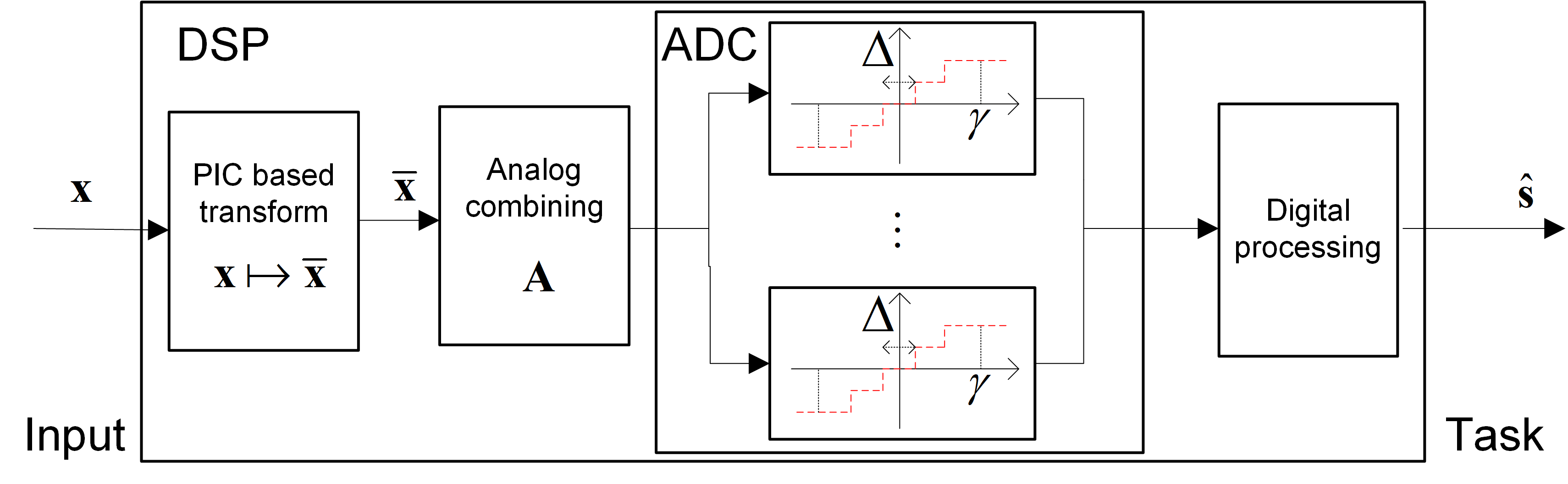
Although Theorem 4 specifically considers functionals $f({{\boldsymbol{x}}})$ of a quadratic form, analogous schemes could be constructed for broader classes of functions. The main feature of Theorem 4 is the ability to represent $\mathbb{E}\{f({{\boldsymbol{x}}})|{{\boldsymbol{z}}}\}$ either exactly, or possibly approximately, as a linear function of ${{\boldsymbol{z}}}={\boldsymbol{A}}h({{\boldsymbol{x}}})$ for some transformation $h(\cdot)$. Once the analog mapping satisfies this request, Theorem 3 can be applied to optimize the overall recovery accuracy of the quantization system. Formulated in terms of pic, the choice of $h(\cdot)$ imposes structure on the joint distribution $({{\boldsymbol{x}}},{{\boldsymbol{z}}})$. Consequently, when the task is to recover a function $f({{\boldsymbol{x}}})$ which can be decomposed using pic as $f({{\boldsymbol{x}}})=\sum\alpha_{i}f_{i}({{\boldsymbol{x}}})$, any analog processing which results in ${{\boldsymbol{z}}}$ such that

would allow to design the analog pre-quantization step using existing tools derived for setups in which the mmse estimate is linear. This implies that when recovering some function $f({{\boldsymbol{x}}})$, the structure of the analog mapping should be designed as to yield linear basis functions $g_{i}({{\boldsymbol{z}}})$, allowing the resulting system to be optimized using Theorem 3.

To demonstrate the ability of the proposed design to yield accurate task-based quantizers, we simulate an empirical covariance estimation scenario. Here, the input is given by ${{\boldsymbol{x}}}=[{\boldsymbol{v}}_{1}^{T},\ldots{\boldsymbol{v}}_{4}^{T}]^{T}$, where $\{{\boldsymbol{v}}_{i}\}_{i=1}^{4}$ are i.i.d. $3\times 1$ zero-mean Gaussian random vectors, i.e., $n=12$. The entries of the covariance matrix of ${\boldsymbol{v}}_{i}$, denoted ${\boldsymbol{\Sigma}}_{{\boldsymbol{v}}}$, are $\left({\boldsymbol{\Sigma}}_{{\boldsymbol{v}}}\right)_{i,j}=e^{-|i-j|}$. The parameter of interest is the $3\times 3$ empirical covariance matrix $\frac{1}{4}\sum_{i=1}^{4}{\boldsymbol{v}}_{i}{\boldsymbol{v}}_{i}^{T}$, which is completely determined by its upper triangular matrix, stacked as the desired vector $\tilde{{{\boldsymbol{s}}}}$, thus $k=6$. For the considered scenario, we evaluate the mse achievable by the task-based quanziation system of Fig. 8 where the analog combiner, quantization support, and digital processing are obtained via Theorem 3. The task-based quantizer is compared to recovering the empirical covariance in analog, as well as to directly quantizing ${{\boldsymbol{x}}}$, i.e., a task-ignorant scalar quantizer, and a hybrid system utilizing linear analog combiners based on [12, Sec. V]. For all the above systems, in order to avoid overloading the quantizers, the support is set to $\eta$ times the maximal sum of the standard deviation and absolute mean value of the entries of the input to the adc, where we let $\eta$ increase linearly with the number of bits in the range $[3,6.5]$. The achievable mse versus the number of bits are depicted in Fig. 9.

Observing Fig. 9, we note that the task-based quantizer, which is designed to balance the quantization and estimation errors, achieves the best mse performance. Quantizing $\tilde{{{\boldsymbol{s}}}}$ directly results in notable quantization errors when operating with a small number of bits, due to the need to set the support to a relatively large value resulting in coarse quantization. This demonstrates how the task-based quantization design proposed in Section III-B for linear tasks can be extended to apply for recovering non-linear functions.

Deep task-based quantization operates in a data-driven manner, learning the analog transformation, quantization mapping, and digital processing, from a training data set, consisting of $t$ independent realizations of ${\boldsymbol{s}}$ and ${\boldsymbol{x}}$, denoted $\{{\boldsymbol{s}}^{(i)},{\boldsymbol{x}}^{(i)}\}_{i=1}^{t}$. In general, the training samples may be taken from a set of joint distributions, and not only from the true (unknown) joint distribution of ${\boldsymbol{s}}$ and ${\boldsymbol{x}}$. Here, the analog pre-quantization mapping and the digital post-quantization processing are parameterized as layers of a dnn, as illustrated in Fig. 10. By doing so, the overall task-based quantization system, including the analog combining, quantization rule, and digital processing, can be trained from data in an end-to-end manner using e.g., sgd (sgd). While the proposed system focuses only on the quantization aspect of adc, the resulting design approach can be extended to account also for sampling in addition to quantization, as considered in [30].

In the proposed architecture, the scalar adc, which implements the continuous-to-discrete mapping, is modeled as an activation function between two intermediate layers, interfacing the analog processing and the digital part. The trainable parameters of this activation function determine the quantization rule, allowing it to be learned during training. The dnn structure cannot contain any skip connections between the multiple layers prior to quantization (analog domain) and those after quantization (digital domain), representing the fact that all analog values must be first quantized before processed in digital. The pre and post quantization networks are henceforth referred to as the analog dnn and the digital dnn, respectively. The system input is the observed ${\boldsymbol{x}}$, and we use ${\boldsymbol{\theta}}$ to denote the network parameters. Two families of tasks are considered:

• •

  Estimation: Here, the system should learn to recover a set of $k$ unknown parameters taking values on a continuous set, i.e., $\mathcal{S}=\mathcal{R}$. By letting $\psi_{{\boldsymbol{\theta}}}(\cdot)$ denote the mapping implemented by the overall system, the output is given by the $k\times 1$ vector $\hat{{\boldsymbol{s}}}=\psi_{{\boldsymbol{\theta}}}({\boldsymbol{x}})$, which is used as a representation of ${\boldsymbol{s}}$. The loss function is the empirical mse:

  $$\mathcal{L}({\boldsymbol{\theta}})=\frac{1}{t}\sum_{j=1}^{t}\left\|{{\boldsymbol{s}}}^{\left(j\right)}-\psi_{{\boldsymbol{\theta}}}\Big({\boldsymbol{x}}^{(j)}\Big)\right\|_{2}^{2}.\vskip-5.69046pt$$

  (6)

• •

  Classification: In such tasks, the system should decide between a finite number of options. Here, $\mathcal{S}$ is a finite set, and we use $|\mathcal{S}|$ to denote its cardinality. The last layer of the digital dnn is a softmax layer, and thus the network mapping $\psi_{{\boldsymbol{\theta}}}(\cdot)$ is a $|\mathcal{S}|^{k}\times 1$ vector, whose entries represent the conditional probability for each different value of ${\boldsymbol{s}}$ given the input ${\boldsymbol{x}}$. By letting $\psi_{{\boldsymbol{\theta}}}({\boldsymbol{x}};{\boldsymbol{\alpha}})$ be the output value corresponding to ${\boldsymbol{\alpha}}\in\mathcal{S}^{k}$, the decision is selected as the most probable one, i.e., $\hat{{\boldsymbol{s}}}=\arg\max_{{\boldsymbol{\alpha}}\in\mathcal{S}^{k}}\psi_{{\boldsymbol{\theta}}}({\boldsymbol{x}};{\boldsymbol{\alpha}})$. The loss function is the empirical cross-entropy:

  $$\mathcal{L}({\boldsymbol{\theta}})=\frac{1}{t}\sum_{j=1}^{t}-\log\psi_{{\boldsymbol{\theta}}}\Big({\boldsymbol{x}}^{(j)};{\boldsymbol{s}}^{(j)}\Big).\vskip-5.69046pt$$

  (7)

The proposed architecture implements scalar quantization as an intermediate activation in a joint analog-digital hybrid dnn. This layer converts its continuous-amplitude input into a discrete quantity. The non-differentiable nature of such continuous-to-discrete mappings induces a challenge in applying sgd for optimizing the network parameters. In particular, quantization activation, which can be modeled as a superposition of step functions determining the continuous regions jointly mapped into a single value, nullifies the gradient of the cost function. Thus, straight-forward application of sgd with back-propagation fails to properly set the pre-quantization network.

This challenge can be tackled by approximating the non-differentiable quantization mapping by a differentiable one, as proposed in [36]. This is achieved by replacing the continuous-to-discrete transformation with a non-linear activation function which has approximately the same behavior as the quantizer. Specifically, we use a sum of shifted hyperbolic tangents, which are known to closely resemble step functions in the presence of large magnitude inputs. The resulting scalar quantization mapping is given by:

where $\{a_{i},b_{i},c_{i}\}$ are real-valued parameters. When the parameters $\{c_{i}\}$ increase, the corresponding hyperbolic tangents approach step functions.

In addition to learning the weights of the analog and digital dnn, this approach allows to learn the quantization function, and particularly, the best suitable constants $\{a_{i}\}$ and $\{b_{i}\}$. These tunable parameters are later used to determine the decision regions of the scalar quantizer, where the set $\{b_{i}\}$ is used for the decision regions limits while $\{a_{i}\}$ determines the corresponding discrete values assigned to each decision region. The parameters $\{c_{i}\}$, which essentially control the resemblance of (8) to an actual continuous-to-discrete mapping, do not reflect on the quantization rule, and are thus not learned from training. The proposed optimization is achieved by including the parameters $\{a_{i},b_{i}\}$ as part of the network trainable parameters ${\boldsymbol{\theta}}$. Due to the differentiability of (8), one can now apply standard sgd with back-propagation to optimize the overall network, including the analog and digital dnn as well as the quantization rule, in an end-to-end manner. Once training is concluded, the learned $\tilde{q}(\cdot)$ activation (8) is replaced with a scalar quantization mapping dictated by the tunable parameters $\{a_{i},b_{i}\}$. An illustration of how the differentiable mapping (8) is converted into a continuous-to-discrete quantization rule is depicted in Fig. 11. The dashed smooth curve in Fig. 11 represents the differentiable function after training is concluded, and the straight curve is the resulting scalar quantizer.

We next numerically demonstrate the achievable performance of deep task-based quantization. In the following, we model the relationship between the observed ${{\boldsymbol{x}}}$ and the task ${{\boldsymbol{s}}}$ as

for some fixed ${\boldsymbol{H}}\in\mathcal{R}^{n\times k}$, where ${\boldsymbol{w}}\in\mathcal{R}^{n}$ is a zero-mean Gaussian vector with i.i.d. entries of variance $\sigma_{w}^{2}>0$.

We begin with an estimation task for which we can compare the data-driven task-based system to its model-aware counterpart detailed in Section III-B. Here, we set $\sigma_{w}^{2}=0.25$, $n=120$, $k=40$, while ${{\boldsymbol{s}}}$ is a zero-mean Gaussian vector with i.i.d. unit variance entries. The matrix ${\boldsymbol{H}}$ is set to

where ${\boldsymbol{\Phi}}$ is the first $4$ columns of the $12\times 12$ dft matrix. This setting represents channel estimation in Rayleigh fading mimo channels using orthogonal pilots [15, Sec. IV]. In Fig. 13 we numerically evaluate the average mse versus the quantization rate $R$ of deep task-based quantization compared to the fundamental performance limit dictated by indirect rate-distortion theory, as well as to the performance of the model-aware task-based quantizer discussed in Section III. To guarantee fair comparison with the model-aware system we set the pre and post quantization dnn to consist of linear layers. Following [12, Prop. 2], we set the number of scalar quanizers to $p=k$ for both task-based quantizers. The data-driven system is trained using $t=2^{15}$ labeled pairs, and all systems are tested using $2^{10}$ test samples. We also depict in Fig. 13 the average mse of a task-ignorant system in which estimation is carried out only in the digital domain, using the method for channel estimation from quantized measurements proposed in [8].

Observing Fig. 13, we note that the fact that data-driven quantizer is not restricted to uniform quantizers allows it to outperform the model-aware system of Section III especially in lower quantization rates. Furthermore, the performance of both task-based quantizers is within a relatively small gap of the fundamental performance limits. These results demonstrate the ability of deep task-based quantization to implement a feasible and optimal-approaching quantization system in a data-driven fashion.

Next, we consider a classification task. Again, the observations ${{\boldsymbol{x}}}$ are related to the task vector ${{\boldsymbol{s}}}$ via (9). However, here the entries of ${{\boldsymbol{s}}}$ are i.i.d. uniformly distributed over $\mathcal{S}=\{-1,1\}$ representing, e.g., symbol detection in mimo communications. In particular, we use $n=12$, $k=4$, and set the entries of ${\boldsymbol{H}}$ to $({\boldsymbol{H}})_{i,j}=e^{-|i-j|}$. For the deep task-based quantizer we use two fully-connected layers in analog and two fully-connected layers in digital. As this is a classification task, the output layer is a softmax function with $2^{k}$ probabilities, and the overall network is trained to minimize the cross-entropy loss (7) using $t=5000$ labeled samples. Unlike the estimation task for which the number of quantizers $p$ can be set according to the analytical results in [12], here this value was determined based on empirical evaluations. In particular, we use $p=\lfloor kR\rfloor$, resulting in each scalar quantizer using at least $n/k=3$ bits in the hybrid system.

The numerically computed ber (ber) averaged over $20000$ trials versus the snr (snr) defined as $1/\sigma_{w}^{2}$ of the deep task-based quantizer with quantization rate $R=1$ is depicted in Fig. 13 compared to the map (map) rule operating for recovering ${{\boldsymbol{s}}}$ from ${{\boldsymbol{x}}}$, i.e., without quantization constraints, as well as the map rule for recovering ${{\boldsymbol{s}}}$ from a uniformly quantized ${{\boldsymbol{x}}}$ with rate $R=1$, representing a task-ignorant digital only system. It is noted that the map detectors require prior knowledge of ${\boldsymbol{H}}$ or $\sigma_{w}^{2}$, while the data-driven quantizer is invariant of the underlying model and learns its mapping from training. In order to study the resiliency of deep task-based quantization to inaccurate training, we also compute the ber under csi (csi) uncertainty, namely, when the training samples are randomized from a joint distribution of ${\boldsymbol{s}},{\boldsymbol{x}}$ in which the entries of the matrix ${\boldsymbol{H}}$ in (9) are corrupted by additive i.i.d. Gaussian noise, whose variance is $20\%$ the magnitude of the corresponding entry. For comparison, we also evaluate the ber of the map rule with the same level of csi uncertainty.

Observing Fig. 13, we note that in the presence of accurate csi, the ber of our deep task-based quantizer is comparable to that achievable using the map rule operating without quantization constraints. For comparison, the quantized map rule, which operates only in the digital domain, achieves significantly worse ber performance compared to the hybrid deep task-based quatizer, demonstating the benefit of applying pre-quantization processing in the analog domain in order to utilize more accurate quantization while keeping the semantic information required to carry out the task. The results in Fig. 13 also demonstrate the improved robustness of the data-driven system to inaccurate csi. The performance of the model-based map detector is very sensitive to csi uncertainty, resulting in a notable increase in ber due to the model mismatch. However, the performance of the deep task-based quantizer trained under csi uncertainty is within an snr gap of approximately $0.5-2$ dB from its performance when trained using accurate csi. This demonstrates the gains of using dnn for overcoming the sensitivity of model-based approaches to inaccurate model knowledge.

A common strategy to implement mimo receivers, particularly when equipped with a large number of antennas and when operating in high spectral bands, is to introduce dedicated analog circuitry between the antennas and the adc. The original motivation for implementing such hybrid receivers is to reduce the number of costly RF chains, namely, the main purpose of the analog combiner is to reduce the dimensionality of the acquired signals allowing the receiver to operate with less RF chains than antennas [19, 20]. The typical implementation of such analog combiners is based on an inter-connection of phase shifters and adders, either connecting a controllable phase-shifted version of the signal observed at each antenna to each adc, resulting in a fully-connected phase shifter network, or alternatively, by dividing the antennas into subsets, each phase shifted and connected to a distinct adc, a topology referred to as partially-connected phase shifter network [20].

The resulting system model of a hybrid mimo receiver thus includes an additional linear processing prior to acquisition, similarly to the model used in our derivation in Section III-B, and can thus be exploited for realizing task-based quantization. In particular, for a hybrid receiver with a fully-connected phase shifter network, the resulting matrix ${\boldsymbol{A}}$ in Section III-B is subject to an additional constraint which stems from the usage of adjustable phase shifters, that only the phase of its entries can be configured, i.e., $|({\boldsymbol{A}})_{i,j}|=1$ for each $i\in\{1,\ldots,p\}$ and $j\in\{1,\ldots,n\}$. This constraint can accounted for by identifying the unconstrained analog combining matrix via, e.g., Theorem 3, and projecting it to the feasible set of fully-connected phase shifter networks, similarly to [20, Alg. 2]. Alternatively, when using a data-driven design as proposed in Section IV, one can account for the additional design constraints by letting the trainable parameters of the analog network to be the phases of the entries of the matrix ${\boldsymbol{A}}$.

The difficulties associated with using phase shifter networks as analog combiners for task-based quantization can be mitigated by introducing adjustable gains into the analog circuitry. For example, the prototype proposed in [21], depicted in Fig. 14, implements a complex-gain analog combiner operating in the sub-$6$ GHz band using digitally controllable vector multipliers. A controllable gain analog combiner operting in the $25-30$ GHz band based on RF integrated circuits was proposed in [37]. The resulting model of a hybrid receiver equipped with such analog combiners effectively allows to control both the gain and phase of each entry of the matrix ${\boldsymbol{A}}$ individually in run-time, thus allowing to implement the task-based quantization systems proposed in the previous sections. The main drawback of such implementations compared to phase shifter networks is the cost and complexity associated with controllable complex gain analog circuits.

The analog combiners discussed in the previous section require the mimo receiver to be equipped with a dedicated analog combining hardware interfacing its antenna elements and the adc. An alternative strategy to realize configurable analog combining without requiring additional dedicated circuitry is to implement the pre-quantization processing as part of the antenna architecture, by using dma. The conventional gains of such metasurfaces over architectures based on standard antenna arrays stem from the fact metasurfaces typically use much less power and cost less [38], while facilitating the implementation of a large number of elements in a given physical area. An additional gain of dma noted in [22] is their ability to implement tunable combining as an inherent byproduct of the antenna architecture.

In particular, dma consist of a set of microstrips, each embedded with configurable radiating metamaterial elements [39]. When used as a receive antenna, the signals observed by the elements are captured at a single output port for each microstrip, feeding an adc. The relationship between these signals and the micropstip output is dictated by two main properties: $1)$ Each element of index $l$ of microstrip $i$ acts as resonant electrical circuit, whose frequency response is described by the Lorentzian form [39]

where $F_{i,l}$, $\chi_{i,l}$, and $\omega_{i,l}^{R}$ are the oscillator strength, damping factor, and angular resonance frequency, respectively, which are all externally configurable parameters. $2)$ Each signal which propagates from an element to the output port undergoes a different path, and thus accumulates a different delay. The delay accumulated by the signal captured at the $l$th element of the $i$th micropstrip can be modeled as a filter with frequency response $h_{i,l}(\omega)$. The signal observed at the output port of the $i$th micrtopstrip can thus be written as the sum of outputs of the filters $b_{i,l}(\omega)h_{i,l}(\omega)$ whose inputs are the signals observed by the corresponding elements, as illustrated in Fig. 15.

The resulting model relating the observed signals and the dma output ports, which are the signals fed to the adc, represents a form of frequency-selective analog combining. Specifically, the fact that the parameters of the Lorentzian response in (10) can be modified element-wise, indicates that the inherent processing carried out inside each micropstrip can be tuned to facilitate acquisition under bit constraints by tuning the resulting combining as part of a task-based quantizer, see, e.g., [23]. Consequently, when using a mimo receiver with a dma-based antenna array, one can implement a form of task-based quantization without requiring additional dedicated analog combining hardware by properly tuning the frequency response of each element along with the quantization mapping and the digital processing utilizing either of the methods discussed in Sections III-IV.

The architectures detailed in this section can all be used to realize task-based quantization in mimo receivers, by exploiting either the model-aware design guidelines proposed in Section III, or alternatively, by learning the task-based quantization mapping from labeled data as suggested in Section IV. Combining the architectures detailed in this section with the design methods proposed in the previous sections thus narrows the gap between the theory of task-based quantization and its concrete implementation in mimo receivers.

References

- [1] T. L. Marzetta, “Noncooperative cellular wireless with unlimited numbers of base station antennas,” IEEE Trans. Wireless Commun., vol. 9, no. 11, p. 3590, 2010.
- [2] N. Shlezinger and Y. C. Eldar, “On the spectral efficiency of noncooperative uplink massive MIMO systems,” IEEE Trans. Commun., vol. 67, no. 3, pp. 1956–1971, 2019.
- [3] J. G. Andrews, S. Buzzi, W. Choi, S. V. Hanly, A. Lozano, A. C. Soong, and J. C. Zhang, “What will 5G be?” IEEE J. Sel. Areas Commun., vol. 32, no. 6, pp. 1065–1082, June 2014.
- [4] R. H. Walden, “Analog-to-digital converter survey and analysis,” IEEE J. Sel. Areas Commun., vol. 17, no. 4, pp. 539–550, 1999.
- [5] Y. C. Eldar, Sampling theory: Beyond bandlimited systems. Cambridge University Press, 2015.
- [6] J. Mo, P. Schniter, and R. W. Heath, “Channel estimation in broadband millimeter wave MIMO systems with few-bit ADCs,” IEEE Trans. Signal Process., vol. 66, no. 5, pp. 1141–1154, 2017.
- [7] Y. Li, C. Tao, G. Seco-Granados, A. Mezghani, A. L. Swindlehurst, and L. Liu, “Channel estimation and performance analysis of one-bit massive MIMO systems,” IEEE Trans. Signal Process., vol. 65, no. 15, pp. 4075–4089, 2017.
- [8] S. Jacobsson, G. Durisi, M. Coldrey, U. Gustavsson, and C. Studer, “Throughput analysis of massive MIMO uplink with low-resolution ADCs,” IEEE Trans. Wireless Commun., vol. 16, no. 6, pp. 4038–4051, 2017.
- [9] J. Choi, J. Mo, and R. W. Heath, “Near maximum-likelihood detector and channel estimator for uplink multiuser massive MIMO systems with one-bit ADCs,” IEEE Trans. Commun., vol. 64, no. 5, pp. 2005–2018, 2016.
- [10] H. Pirzadeh and A. L. Swindlehurst, “Spectral efficiency of mixed-ADC massive MIMO,” IEEE Trans. Signal Process., vol. 66, no. 13, pp. 3599–3613, 2018.
- [11] S. Khobahi, N. Naimipour, M. Soltanalian, and Y. C. Eldar, “Deep signal recovery with one-bit quantization,” in Proc. IEEE ICASSP, 2019.
- [12] N. Shlezinger, Y. C. Eldar, and M. R. Rodrigues, “Hardware-limited task-based quantization,” IEEE Trans. Signal Process., vol. 67, no. 20, pp. 5223–5238, 2019.
- [13] ——, “Asymptotic task-based quantization with application to massive MIMO,” IEEE Trans. Signal Process., vol. 67, no. 15, pp. 3995–4012, 2019.
- [14] S. Salamatian, N. Shlezinger, Y. C. Eldar, and M. Médard, “Task-based quantization for recovering quadratic functions using principal inertia components,” in Proc. IEEE ISIT, 2019.
- [15] N. Shlezinger and Y. C. Eldar, “Deep task-based quantization,” arXiv preprint arXiv:1908.06845, 2019.
- [16] F. P. Calmon, A. Makhdoumi, M. Médard, M. Varia, M. Christiansen, and K. R. Duffy, “Principal inertia components and applications,” IEEE Trans. Inf. Theory, vol. 63, no. 8, pp. 5011–5038, 2017.
- [17] M. R. Rodrigues, N. Deligiannis, L. Lai, and Y. C. Eldar, “Rate-distortion trade-offs in acquisition of signal parameters,” in Proc. IEEE ICASSP, 2017, pp. 6105–6109.
- [18] K. Yu, Y. D. Zhang, M. Bao, Y.-H. Hu, and Z. Wang, “DOA estimation from one-bit compressed array data via joint sparse representation,” IEEE Signal Process. Lett., vol. 23, no. 9, pp. 1279–1283, 2016.
- [19] R. Méndez-Rial, C. Rusu, N. González-Prelcic, A. Alkhateeb, and R. W. Heath, “Hybrid MIMO architectures for millimeter wave communications: Phase shifters or switches?” IEEE Access, vol. 4, pp. 247–267, 2016.
- [20] S. S. Ioushua and Y. C. Eldar, “A family of hybrid analog–digital beamforming methods for massive MIMO systems,” IEEE Trans. Signal Process., vol. 67, no. 12, pp. 3243–3257, 2019.
- [21] T. Gong, N. Shlezinger, S. S. Ioushua, M. Namer, Z. Yang, and Y. C. Eldar, “RF chain reduction for MIMO systems: A hardware prototype,” arXiv preprint arXiv:1905.05315, 2019.
- [22] N. Shlezinger, O. Dicker, Y. C. Eldar, I. Yoo, M. F. Imani, and D. R. Smith, “Dynamic metasurface antennas for uplink massive MIMO systems,” IEEE Trans. Commun., vol. 67, no. 10, pp. 6829–6843, 2019.
- [23] H. Wang, N. Shlezinger, Y. C. Eldar, S. Jin, M. F. Imani, I. Yoo, and D. R. Smith, “Dynamic metasurface antennas for MIMO-OFDM receivers with bit-limited ADCs,” arXiv preprint arXiv:1912.06917, 2019.
- [24] R. M. Gray and D. L. Neuhoff, “Quantization,” IEEE Trans. Inf. Theory, vol. 44, no. 6, pp. 2325–2383, 1998.
- [25] T. M. Cover and J. A. Thomas, Elements of information theory. John Wiley & Sons, 2012.
- [26] R. M. Corey and A. C. Singer, “Wideband source localization using one-bit quantized arrays,” in Proc. IEEE CAMSAP, 2017.
- [27] H. Witsenhausen, “Indirect rate distortion problems,” IEEE Trans. Inf. Theory, vol. 26, no. 5, pp. 518–521, 1980.
- [28] J. Wolf and J. Ziv, “Transmission of noisy information to a noisy receiver with minimum distortion,” IEEE Trans. Inf. Theory, vol. 16, no. 4, pp. 406–411, 1970.
- [29] Y. Polyanskiy and Y. Wu, “Lecture notes on information theory,” 2015.
- [30] N. Shlezinger, R. J. G. van Sloun, I. A. M. Hujiben, G. Tsintsadze, and Y. C. Eldar, “Learning task-based analog-to-digital conversion for MIMO receivers,” in Proc. IEEE ICASSP, 2020.
- [31] R. M. Gray and T. G. Stockham, “Dithered quantizers,” IEEE Trans. Inf. Theory, vol. 39, no. 3, pp. 805–812, 1993.
- [32] B. Widrow, I. Kollar, and M.-C. Liu, “Statistical theory of quantization,” IEEE Trans. Instrum. Meas., vol. 45, no. 2, pp. 353–361, 1996.
- [33] D. P. Palomar and Y. Jiang, “MIMO transceiver design via majorization theory,” Foundations and Trends® in Communications and Information Theory, vol. 3, no. 4-5, pp. 331–551, 2007.
- [34] V. Kostina and S. Verdú, “Nonasymptotic noisy lossy source coding,” IEEE Trans. Inf. Theory, vol. 62, no. 11, pp. 6111–6123, 2016.
- [35] W. C. Jakes and D. C. Cox, Microwave mobile communications. Wiley-IEEE Press, 1994.
- [36] E. Agustsson, F. Mentzer, M. Tschannen, L. Cavigelli, R. Timofte, L. Benini, and L. V. Gool, “Soft-to-hard vector quantization for end-to-end learning compressible representations,” in Advances in Neural Information Processing Systems, 2017, pp. 1141–1151.
- [37] S. Mondal, R. Singh, A. I. Hussein, and J. Paramesh, “A 25–30 GHz fully-connected hybrid beamforming receiver for MIMO communication,” IEEE J. Solid-State Circuits, vol. 53, no. 5, pp. 1275–1287, 2018.
- [38] M. C. Johnson, S. L. Brunton, N. B. Kundtz, and J. N. Kutz, “Sidelobe canceling for reconfigurable holographic metamaterial antennas,” IEEE Trans. Antennas Propag., vol. 63, no. 4, pp. 1881–1886, Apr. 2015.
- [39] D. R. Smith, O. Yurduseven, L. Pulido-Mancera, P. Bowen, and N. B. Kundtz, “Analysis of a waveguide-fed metasurface antenna,” Phys. Rev. Applied, vol. 8, no. 5, Nov. 2017.