Secure Millimeter Wave Cloud Radio Access Networks Relying on Microwave Multicast Fronthaul
Abstract
In this paper, we investigate the downlink secure beamforming (BF) design problem of cloud radio access networks (C-RANs) relying on multicast fronthaul, where millimeter-wave and microwave carriers are used for the access links and fronthaul links, respectively. The base stations (BSs) jointly serve users through cooperating hybrid analog/digital BF. We first develop an analog BF for cooperating BSs. On this basis, we formulate a secrecy rate maximization (SRM) problem subject both to a realistic limited fronthaul capacity and to the total BS transmit power constraint. Due to the intractability of the non-convex problem formulated, advanced convex approximated techniques, constrained concave convex procedures and semi-definite programming (SDP) relaxation are applied to transform it into a convex one. Subsequently, an iterative algorithm of jointly optimizing multicast BF, cooperative digital BF and the artificial noise (AN) covariance is proposed. Next, we construct the solution of the original problem by exploiting both the primal and the dual optimal solution of the SDP-relaxed problem. Furthermore, a per-BS transmit power constraint is considered, necessitating the reformulation of the SRM problem, which can be solved by an efficient iterative algorithm. We then eliminate the idealized simplifying assumption of having perfect channel state information (CSI) for the eavesdropper links and invoke realistic imperfect CSI. Furthermore, a worst-case SRM problem is investigated. Finally, by combining the so-called -Procedure and convex approximated techniques, we design an efficient iterative algorithm to solve it. Simulation results are presented to evaluate the secrecy rate and demonstrate the effectiveness of the proposed algorithms.
Index Terms:
Multicast, C-RAN, millimeter-wave communication, physical layer security.I Introduction
To satisfy the ever-increasing demand for higher data rates, cloud radio access networks (C-RANs) have been proposed as promising solutions, where the base stations (BSs) are connected to a central processor (CP) such as the mobile switching center through limited-capacity fronthaul links [1], [2]. In C-RANs, the CP performs sophisticated baseband signal processing and resource optimization by exploiting global channel state information (CSI) for significantly reducing the interference among users, while improving the spectral efficiency (SE) of the system [3]. Additionally, with the deployment of ultra-dense BSs, it becomes beneficial for the adjacent BSs to form a BS cluster and to cooperatively/jointly serve users relying on the sophisticated coordinated multiple-point (CoMP) transmission approach [4].
The CoMP-based C-RAN structure of Fig. 1 generally includes a CP, cooperating BSs and users. The BSs receive data from the CP via the fronthual links, while the users are jointly served by the BSs via cooperative beamforming (BF). Thus, a pair of fundamental problems have to be considered, namely: the fronthaul/access links and the data sharing approach. For the former, in general, there are multiple carrier technologies that can be adopted, such as tethered links relying on fiber or copper, and wireless links using microwave or millimeter-wave (mmWave) carriers [5]-[7]. However, for the ultra-dense BS deployment, it would be unrealistic to have a wired connection between each BS and the CP due to its high cost. Furthermore, the capacity provided by wired links is fixed, hence it cannot be dynamically adjusted to cater for the traffic variation according to the users’ demands. Therefore, the more flexible wireless carriers constitute appropriate candidates for fronthaul links [8]. Here, we adopt the microwave fronthaul-link carriers and mmWave access-link carriers, and the reason as follows: The distance between the CP and the BSs is relatively high, hence it is inefficient to use mmWave frequencies due to their high propagation loss. Therefore we adopted a microwave fronthaul as a benefit of its lower path-loss. Additionally, although the propagation loss of mmWave signals is high, the distance between the BSs and users is relatively short, hence it is appropriate to use mmWave access links. Furthermore, these choices avoid the interference between the fronthaul and access links. As for the data sharing approach among the CP and BS cluster, when multiple BSs jointly serve a user, the CP needs to transmit this user’s message to all the cooperating BSs. Fortunately, this point-to-multipoint CP-BSs fronthaul transmission can be readily realized by multicast BF, which has been applied in [9], [10]. Therefore, in this paper, we will formulate a more practical system relying on BS-cooperation-aided mmWave C-RAN combined with a microwave multicast fronthaul.
Additionally, due to the broadcast nature of wireless communication, the users’ confidential messages may be eavesdropped, jeopardizing their secure transmissions [11]-[15]. As a compelling solution, physical layer security (PLS) has been proposed for enhancing the communication security [16]. Although numerous solutions have been conceived for PLS [11]-[16], the following challenges exist in our proposed system structure. i) Hybrid analog/digital BF design: The BSs are usually equipped with multiple mmWave antennas to compensate for the serious propagation loss. However, in order to reduce the radio frequency (RF) energy consumption and hardware cost, only a few RF chains are affordable [17]. For this reason, we consider hybrid analog/digital BF designs for the cooperating BSs. ii) Artificial noise (AN) design: To further improve the transmission security, the AN used for jamming should be properly designed for the cooperating BSs. iii) Multicast BF design: The CP-BSs multicast BF has to be optimally designed for improving the fronthaul capacity.
Against this background, in this paper, we investigate the downlink (DL) transmission security problem of a mmWave C-RAN with multicast fronthaul. Our main contributions include:
- •
We propose a BS-cooperation-aided C-RAN relying on a microwave multicast fronthaul. The adjacent BSs form a cooperating cluster and jointly serve the users relying on mmWave carriers, while the BSs receive their fronthaul data from the CP with microwave multicast. To reduce both the hardware cost and energy consumption, each BS is equipped with a single RF chain connected to multiple antennas. This scenario is further complicated by the fact that the eavesdroppers (Eves) maliciously attack the legitimate users in order to wiretap their confidential messages.
- •
We design a DL analog transmit BF scheme for the cooperating BSs. Based on an equivalent channel model, we formulate a DL secrecy rate maximization (SRM) problem by jointly optimizing the microwave CP-BSs multicast BF, the cooperative mmWave BSs-users digital BF and the AN covariance under the constraints of fronthaul capacity and total BS transmit power. However, the problem formulated is intractable because of its non-convexity. Hence, advanced convex approximated techniques, constrained concave convex procedures (CCCP) and semi-definite programming (SDP) relaxation are applied to recast the original problem into a convex one. Then, we propose an efficient iterative algorithm for solving the original problem. Meanwhile, we construct the solution of the original problem by exploiting both the primal and the dual optimal solution of the SDP-relaxed problem. Next, we replace the total BS transmit power constraint by a per-BS transmit power constraint and reformulate the SRM problem. An iterative solution algorithm is also proposed.
- •
To consider a practical scenario, we then dispense with the idealized simplifying assumption of having perfect CSIs for the Eves links and replace it by realistic imperfect CSIs ones followed by investigating a worst-case SRM problem. The problem formulated is then solved by our proposed iterative algorithm relying on the classic -Procedure and the convex approximated techniques. Our simulation results demonstrate the efficiency of the proposed algorithms.
The rest of this paper is organized as follows. The related contributions are summarized in Section II. The systems description and the analog BF designed are presented in Section III. In Section IV, the SRM problem formulated both under total BS and under per-BS transmit power constraints are solved, respectively. A realistic imperfect CSI is considered for the Eves links in Section V. Our simulation results are drawn in Section VI. Finally, we conclude this paper in Section VII.
Notations: We use the following notations throughout this paper: and denote the transpose and Hermitian transpose, respectively, is the Frobenius norm, means the space of complex matrix, Re() and Tr() denote real number operation and trace operation, respectively. denotes the , and Diag() is a diagonal matrix.
II Related Works
II-A Physical Layer Security in mmWave Communications
In [18], Wang et al. invoke both the maximum ratio transmit BF and AN BF for improving the secrecy capacity, and derive the closed-form expression of the connection probability. Additionally, the throughput is maximized under outage probability constraints. Alotaibi and Hamdi [19] propose a switched phased-array antenna structure for enhancing the secrecy transmission. On this basis, the authors analyze the secrecy capacity and derive the exact expression of the bit error probability. To reduce the hardware cost, Huang et al. [20] consider a pair of sparse RF chain structures and design a directional hybrid analog/digital precoding for substantially improving the secrecy transmission capacity. Relying on a uniform linear array at the BS, Zhu et al. propose a tractable technique for evaluating the secrecy rate, when exploiting the AN [21]. Their research results show that the secrecy performance can be improved at low transmit powers. Sun et al. [22] investigate the secrecy capacity in a simultaneous wireless information and power transfer (SWIPT) network associated with unmanned aerial vehicular (UAV) relays. The closed-form expression of the average secrecy transmission rate is derived for a three-dimensional mmWave antenna model and then, the lower bound of the secrecy transmission rate is maximized. Similarly, Sun et al. [23] consider a secrecy SWIPT-aided mmWave ultra-dense network and derive the energy-information coverage probability as well as the effective secrecy throughput both under power splitting and time switching with the aid of stochastic geometry. Wang et al. [24] consider the PLS of relay-aided mmWave systems and design a two-stage secure hybrid analog/digital precoding scheme.
Although the PLS of mmWave communications has been lavishly investigated in [18]-[24], most authors only analyze the secrecy capacity and derive the related closed-form expressions, such as [18], [19], [22], and [23]. However, there is a paucity of information on the associated BF design and resource optimization. The authors of [20] and [24] do consider the hybrid analog/digital precoding design problem under the idealized assumption of perfect CSI.
II-B Multicast Transmissions in Cloud Radio Access Network
Hu et al. [9] propose to transmit the users’ data from the CP relying on fronthaul multicast, and formulate a joint BF design and user clustering problem for maximizing the weighted sum rate. Then, an iterative binary search algorithm is proposed. A cache-based C-RAN using a multicast backhaul/fronthaul is investigated by Dai et al. [10]. They also formulate a joint BS cache and BF design problem for minimizing the transmission delay and then propose a powerful optimization algorithm. Chen et al. [25] investigate a BF design problem in a multigroup multicast C-RAN relying on limited backhaul capacity, and a robust BF design algorithm is developed for maximizing the worst-user rate. Similar to [25], Tao et al. [26] assume that the users will form a cluster when they request the same content from the CP, hence they are served by the cache-based BS cluster through multicast. They also propose a dynamic BS cache and multicast BF design scheme for minimizing the weighted backhaul cost and transmit power. As a future advance, Vu et al. [27] conceive joint BS selection and BF design for maximizing the minimum weighed data rate under finite-capacity fronthaul links. Based on this, they also develop an upper bound based on the classic semidefinite relaxation technique and propose a heuristic low-complexity iterative algorithm. Shi et al. [28] investigate the power minimization problem by dynamically selecting active BSs under imperfect CSI, and a robust and sparse three-stage BF design algorithm is proposed. To minimize the delivery latency in a cache-based multigroup multicasting network, He et al. [29] develop three transmission schemes and evaluate their performance.
Indeed, substantial research efforts have been invested in designing multicast-aided C-RANs. However, most of them consider fixed-capacity/wired fronthaul links, such as [25]-[29], and multicast transmission is only applied to the access links. Although the authors of [9] and [10] do investigate the multicast fronthaul/backhaul-aided C-RAN, they mainly focus their attention on the caching and transmission delay problem. Furthermore, the specifics of mmWave communication and PLS are not considered in the above contributions.
In contrast to the aforementioned studies, we investigate the transmission security problem in a BS-cooperation-aided mmWave C-RAN relying on a limited-capacity microwave multicast fronthaul. In the system considered, there are two techniques conceived for securing the communication link: Carefully constructed antenna beamforming, and Jamming by artificial noise. More explicitly, beamforming improves the SINR by mitigating the interference, while artificial noise is used for confusing the eavesdropper so as to improve the secure rate. The main contributions of this paper can be summarized from the following three perspectives: Propose a BS-cooperation-aided C-RAN relying on a microwave multicast fronthaul; Develop a joint downlink transmit beamforming design algorithm (i.e., Algorithm 2) for the cooperating BSs under perfect CSI, and analyze the rank characteristic of the solution as well as give the corresponding proof; Investigate a worst-case sum rate maximization problem by considering imperfect CSI knowledge, and propose an efficient beamforming design algorithm (i.e., Algorithm 3).
III System Model and Analog Beamforming Design
In this section, we first describe the system model and mmWave channel model. Then, we propose an analog BF design scheme for cooperating BSs.
III-A System Model
A DL C-RAN relying on a central CP is considered, as shown in Fig. 1. For simplicity, we consider a single BS cluster consisting of cooperating BSs11 1 Although we consider a single BS cluster, the proposed algorithm and analytical results can be extended to multiple BS clusters., where all BSs jointly serve single-antenna users via cooperative mmWave BF. We assume that there are single-antenna Eves potentially overhearing the users’ message. The CP equipped with antennas transmits its signals to the BSs via microwave multicast fronthaul links, and each BS relies on a single receive antenna (RA) and transmit antennas (TAs). Since the BS’s TAs operate at a mmWave frequency, we assume that only a single RF chain serves TAs through a group of quantized phase shifters for reducing both the hardware cost and energy consumption22 2 Since each BS is equipped with a single RF chain, to reduce the inter-user interference, we assume that the number of users being served simultaneously is small than that of BSs. When there are are users, they can be served by time division multiplex access (TDMA) or by appropriate user scheduling [30]. [31]. Additionally, the wireless fronthaul links rely on out-of-band spectrum, hence there is no interference between the access and fronthaul links.

III-A1 Microwave Multicast Fronthaul Link
The signal received at the th BS can be written as
| (1) |
where denotes the fronthaul link’s channel vector from the CP to the th BS, represents the multicast BF vector transmitted by the CP to the BS cluster, and is the multicast signal with . Furthermore, is the independent and identically distributed (i.i.d.) additive white Gaussian noise (AWGN) with zero mean value and follows .
As a result, the achievable fronthaul rate of the th BS is
| (2) |
where denotes the DL microwave bandwidth. Since the fronthaul multicast rate is limited by the BS owning the worst channel condition, the fronthaul rate provided by the CP can be expressed as
| (3) |
where denotes the BS set.
III-A2 Millimeter Wave Access Link
The received signal of the th user can be written as
| (4) |
where represents the DL channel vector from cooperating BSs to the th user, represents the DL channel vector from the th BS to the th user, while is the AN transmitted by the BS cluster. It is assumed that , where denotes the AN covariance matrix to be optimized, while and , respectively, denote the digital BF vector and the signal desired for the th user, and is the i.i.d. AWGN with . is the analog BF, which can be expressed as
where denotes the analog BF vector designed by the th BS and all elements of have the same amplitude but different phases [32], namely , where is the antenna set of each BS and represents the th element of .
Accordingly, the achievable rate of the th user can be expressed as
| (10) |
where denotes the mmWave bandwidth.
On the other hand, the Eves try to intercept the message of the th user, and the signal received at the th Eve can be written as
| (11) |
where denotes the DL channel vector from cooperating BSs to the th Eve, represents the DL channel vector from the th BS to the th Eve. Then, the th Eve can wiretap the th user at a rate of
| (12) |
Finally, the achievable secrecy rate of the th user can be expressed as [33]
| (13) |
where denotes the Eves set.
III-A3 Millimeter Wave Channel Model
In this paper, we adopt the mmWave channel model having scatters, where each scatter includes a single propagation path between the th BS and the th user [34]. Therefore, the mmWave channel can be described as
| (14) |
where denotes the complex gain of the -th path, is the azimuth angle of arrival for the -th path, and represents the antenna array’s steering vector that can be expressed as
| (15) |
where and , respectively, denote the inter-antenna distance and signal wavelength. The channel model of Eves has a similar expression to (10), which is omitted it here.
III-B Analog Beamforming Design For Cooperating BSs
In order to reduce the total complexity of the joint BF (including the analog, digital and multicast BF) design, we first design the analog BF (i.e., ), and then obtain the equivalent mmWave channel. In practice, only a quantized phase can be realized [35]. We assume that -bit quantized phase shifters are used, and the non-zero elements of the analog BF should belong to
| (16) |
According to (III-A2), we need to design the analog BF for BSs, respectively. For the th user, we have , and thus we can maximize the array again by appropriately selecting the optimal quantized phase from (16). For example, for the analog BF vector of the th BS, the th angle of can be selected as
| (17) |
where denotes the angle of , and we have
| (18) |
Additionally, to guarantee user fairness, the BF designed for the BSs should not only maximize the single user’s array gain, and each user should be allocated at least one BS to maximize its array gain. We summarize the analog BF design scheme in Algorithm 1.
while do 1
If then Break. end for 5
IV Secrecy Rate Maximization Problem Formulation and Solution
In this section, we first formulate the SRM problem under the total BS transmit power as well as CP transmit power constraints, and an efficient iterative algorithm is proposed. Then, a per-BS transmit power constraint is considered and a similar SRM algorithm is developed.
IV-A Problem Formulation Under Total BS Transmit Power Constraint
After designing the analog BF , we can achieve the equivalent channel of the th user as . Similarly, the equivalent channel of the th Eve can be expressed as .
We assume that the multicast fronthaul transmission time frame includes slots, and each slot is used to transmit a single user’s message from the CP to cooperating BSs. For simplicity, the frame length and the th slot length are, respectively, assumed to be 1 and , thus we have . According to the specific constraint that the achievable capacity of the th user must be lower than the fronthaul capacity provided by the CP for the th user [36], we have
| (19) |
where denotes the user set. Since and , we can obtain (19) as follows:
| (20) |
Next, we have to state that as long as there is at least one scenario in which we can obtain (19) from (20), then we can find one case from (20) to satisfy the fronthaul capacity constraint. Next, we provide the proof. We rewrite (20) as follows:
| (21) |
Since and , we have
| (22) |
According to (22), we have
| (23) |
Hence, there always exists one case satisfying
| (24) |
which completes the proof.
Finally, we formulate the joint BF and AN variance design problem to maximize the secrecy rate, which can be cast as
| (25a) | ||||
| (25b) | ||||
| (25c) | ||||
| (25d) | ||||
where (25b) denotes the fronthaul capacity constraint, (25c) is the total transmit power constraint of the cooperating BSs, and (25d) represents the CP transmit power constraint. However, it is a challenge to directly solve (25) due to the non-convex nature of the objective function (OF) (25a) and constraint (25b).
IV-B Problem Solution
It is clear that the secrecy rate should not be lower than zero during optimization, otherwise the solution is not meaningful. Therefore, we can move the operation of the OF (25a)33 3 Although is still concave function [37], we move it for convenience.. By introducing the auxiliary variables and , (25a) can be transformed as follows:
| (26) |
with
| (27a) | ||||
| (27b) | ||||
To this end, we define the BF matrix and , and (25) can be reformulated as the following optimization problem
| (28a) | ||||
| (28b) | ||||
| (28c) | ||||
| (28d) | ||||
| (28e) | ||||
| (28f) | ||||
| (28g) | ||||
| (28h) | ||||
where , , and due to . However, problem (28) is still difficult to solve due to (28a)-(28c), (28f) and (25b). To tackle this problem, we first transform (28b) into a convex constraint. By bringing auxiliary variable , we have
| (29a) | ||||
| (29b) | ||||
It is plausible that (29b) is a convex constraint. Additionally, an upper bound of can be obtained as follows [38]:
| (30) |
where and denote the values of and at the th iteration, respectively. We can thus transform (29a) into the following convex constraint
| (31) |
Next, we introduce the auxiliary variables and , and split (28c) into the following constraints
| (32a) | ||||
| (32b) | ||||
| (32c) | ||||
| (40) |
where and denotes other Lagrangian terms that do not affect our analysis.
It can be readily seen that (32a) is a convex constraint. As for (32b), by the first-order Taylor series expansion, the quadratic term can be approximated as
| (33) |
and (32b) can be transformed into the following convex constraint
| (34) |
where denotes the value of at the th iteration. As for the non-linear constraint (32c), we can transform it into the following convex linear matrix inequality (LMI) constraint as
Finally, upon introducing auxiliary variables and , (28) can be transformed into the following optimization problem
| (38a) | ||||
| (38b) | ||||
| (38c) | ||||
| (38d) | ||||
| (38e) | ||||
where , and .
Since and are convex functions, the OF (38a) is constituted by a difference of convex (DC) program [39], and usually CCCP is used to solve the DC program. In fact, the main idea of the CCCP is to transform (38a) into a convex function by approximation, and then the approximated convex problem is iteratively solved until the result converges. Based on this, we consider to use the first-order Taylor approximation for , namely
| (39) |
where denotes the value of at the th iteration. Then, the OF can be transformed into the following convex function
| (40) |
Additionally, one can observe that constraint (38d) is also a DC program. Similarly, we can transform it into the following convex constraint
| (41) |
The non-convex constraint (38b) is yet to be dealt with. Similar to (28c), by bringing auxiliary variable and , (38b) can be split into the following constraints
| (42a) | ||||
| (42b) | ||||
| (42c) | ||||
According to (33)-(IV-B), the non-convex constraints (42b) and (42c) can be formulated the following convex ones
| (43) |
where represents the value of at the th iteration, and
Finally, the SRM problem can be transformed into
| (47a) | ||||
| (47b) | ||||
It is plausible that only the rank-one constraint (28f) is non-convex in (47). By SDP relaxation (i.e., removing the rank-one constraint), (47) will become a convex optimization problem and can be solved by standard convex optimization techniques, such as the interior-point method of [40]. Finally, to obtain the solution of optimization problem (25), we need to iteratively solve (47). Specifically, we first initialize the feasible solution , , , , as well as , and the optimal solution of (47) can be obtained by a classic convex optimization algorithm. Then, , , , , and are updated according to the solution obtained at previous iteration, and problem (47) is resolved until the results converge or the iteration index reaches its maximum value. Additionally, since (47) without rank-one constraint is a convex optimization problem, iteratively updating all variables will increase or at least maintain the value of the OF in (47) [41], [42]. Given the limited transmit power, the value of the OF should be monotonically non-decreasing sequence with an upper bound, which converges to a stationary solution that is at least locally optimal. We summarize the above iterative scheme in Algorithm 2.
Now, we study the rank relaxation problem. To analyze the rank characteristic of the solution, we first define the Lagrangian function of the relaxed version of (47) that can be expressed as (IV-B) at the bottom of this page. Then, we have the following theorems.
Theorem 1
When , let denote an optimal solution of (47), it must hold that
| (41) |
where represents the optimal Lagrange multiplier for the dual problem of (47), while there always exists a so that
| (42) |
Moreover, if there exists any so that , we have
| (43) |
Proof:
Refer to Appendix A. ∎
Theorem 2
Proof:
Refer to Appendix B. ∎
It should be stressed that Theorems 1 and 2 provide only the sufficient conditions for the optimality of the BF. During simulation experience, we found that problem (47) still yields the rank-one solutions even though the above conditions do not hold. However, we still have to consider the following problem: If denotes the optimal solution of problem (47) and there exists or , how can the rank-one solution be obtained? To solve this problem, we consider the following two cases:
repeat 1
Solve the optimization problem (47) without the rank-one constraint and obtain the optimal solution ,
.until or Convergence; 2
IV-C Problem Formulation and Solution Under Per-BS Transmit Power Constraint
In the previous subsection, the total transmit power constraint of BSs is considered. Although the power can be allocated more flexibly to the BSs under total transmit power constraint, each BS is usually prohibited to transmit at high power due to practicality concerns. Therefore, considering per-BS transmit power constraint may be more practical. To this end, we define as
| (45) |
and per-BS power constraint (28d) can be written as
| (46) |
where denotes the maximum transmit power of the th BS. Then, we formulate the following SRM problem under per-BS transmit power constraint as follows:
| (47a) | ||||
| (47b) | ||||
Since (46) is a convex constraint, we can adopt the scheme proposed in Section III. B to deal with problem (47), and finally formulate the following convex optimization problem without a rank-one constraint
| (48a) | ||||
| (48b) | ||||
As a result, we can iteratively solve the above convex optimization problem to obtain the solution of the original problem (47) using a process similar to Algorithm 2. Additionally, we can obtain the similar theorems with Theorems 1 and 2, and the reconstruction of rank-one solution can refer to Appendices A-D.
IV-D Complexity Analysis
We first analyze the complexity of solving (47). Given an iteration accuracy , the number of iterations is on the order , where denotes the threshold parameters related to the constraints [43]. Additionally, (47) includes linear constraints, two-dimensional LMI constraints, one -dimensional LMI constraint, -dimensional LMI constraints and second order cone constraints. Therefore, the complexity of solving (47) is on the order of
| (49) |
where and denotes the number of decision variables, , , . Additionally, one can observe that the only difference between problems (48) and (47) is (46). Since (46) is also a linear constraint, the complexity of solving (48) is on the order of
| (50) |
where , .
V Extension To The Imperfect CSI for Eavesdropper Links
In the previous section, we consider the SRM problem under the assumption that the Eves’ CSIs are perfectly known by the BSs. In fact, since the Eves are usually passive, the BSs cannot obtain their perfect CSIs [44], [45]. Therefore, we assume that the BSs own imperfect CSIs for the Eves links, i.e.,
| (51) |
where is the actual channel vector from BSs to the th Eve, denotes the estimated , and represents the associated CSI error. Here, we assume that the estimation error is bounded and deterministic, which is defined as
| (52) |
where is the error ratio. Hence, the received signal of the th user at the th Eve can be rewritten as
| (53) |
The th Eve has an achievable rate at the th user represented as
| (54) |
where . Then, we can formulate the SRM problem as follows
| (55a) | ||||
| (55b) | ||||
| (55c) | ||||
Observe that problem (55) is similar to (25) except for the wiretap rate and constraint (55b). Therefore, we first deal with these two terms, while the other terms can be transformed into convex ones using the similar methods to that of Section III. B. By introducing auxiliary variable , we reformulate the optimization problem of (55) as
| (56a) | ||||
| (56b) | ||||
| (56c) | ||||
where .
Next, we introduce auxiliary variables , , and split the constraint (56b) into the following ones
| (57a) | ||||
| (57b) | ||||
| (57c) | ||||
| (57d) | ||||
It is observed that (57b) can be transformed into the following convex constraint
| (58) |
where denotes the value of at the th iteration. Additionally, (57c) can be reformulated into the following LMI constraint
| (64) |
| (67) |
where
,
and denotes other Lagrangian terms that do not affect our analysis, , , .
Before dealing with (57a) and (57d), we formulate the following Lemma 1 for the classic -Procedure [46].
Lemma 1
Define the following function
| (62) |
where , ,, and represents any integer. Then, the expression holds if and only if there exists a satisfying
Additionally, (57a) can be rewritten as
| (68) |
According to , (68) can be expressed as the following LMI with Lemma 1
where is the slack variable. Then, we rewrite in (64) at the bottom of the next page. Similar to (68) and (V), combining Lemma 1, (57d) can be expressed as the LMI constraint (V) at the bottom of the next page.
For the OF (56a), and the non-convex constraints (25b) and (28b) in problem (56), the method proposed in Section III. B can be used. To this end, (56) is transformed into the following optimization problem
| (66a) | ||||
| (66b) | ||||
where , , .
The above optimization problem will be convex if there is no rank-one constraint, and it can be solved by standard convex optimization techniques, such as interior-point method. Therefore, by invoking rank-one relaxation, we can iteratively solve (66) to obtain the solution of the original problem (55), following a similar procedure to that of solving problems (47) and (48).
Next, we study the rank relaxation problem. We first define the Lagrangian function of the relaxed version of (66), which is expressed as (V) at the bottom of the next page.
Theorem 3
Proof:
Let us now analyze the complexity of solving (66). Given an iteration accuracy , the number of iterations is on the order , where denotes the threshold parameters related to the constraints [43]. Additionally, (47) includes linear constraints, () two-dimensional LMI constraints, one -dimensional LMI constraint, -dimensional LMI constraints, -dimensional LMI constraints and second order cone constraints. Therefore, the complexity of solving (47) is on the order of
| (69) |
where and denotes the number of decision variables, , , .
| Parameters | Value |
| Number of TAs at the CP | |
| Number of TAs at each BS | |
| Number of the BSs | |
| Number of the users | |
| Number of the Eves | |
| Number of the clusters | |
| Distance between the CP and the BS cluster | 500 [m] |
| Radius of the BS cluster | 30 [m] |
| MmWave bandwidth | [MHz] |
| Microwave bandwidth | [MHz] |
| Standard deviation [47] | [dB] |
| Path loss at the mmWave frequency [47] | [dB] |
| Path loss at the microwave frequency [48] | [dB] |
| Noise variance [26] | -174 [dBm/Hz] |
VI Numerical Results
In this section, numerical results are presented to evaluate the performance of the proposed algorithms. In addition, according to [47], the path-loss of the mmWave channel model can be expressed as: where is the close-in free-space path-loss in dB, is the close-in free-space reference distance, is the best-fit minimum mean square error path-loss exponent over all measurement from a particular measurement campaign, and finally is zero-mean Gaussian random variable with a standard deviation in dB, representing the large-scale signal fluctuations resulting from shadowing owing to obstructions, such as buildings. In our simulations, we set the RF carrier frequency to be 73 GHz, and the reference distance to m. Correspondingly, the path-loss becomes and . The default simulation parameters are listed in Table I. Unless otherwise specified, these default values are used in simulation. The BSs, users and Eves are randomly located in the cell radius following a uniform distribution. The azimuth angle of departure at each BS is uniformly distributed over . Additionally, we assume that the imperfect CSI of all Eves have the same error bound for simplicity. We plot the deployment figure of BSs, users and Eves as showed in Fig. 2.
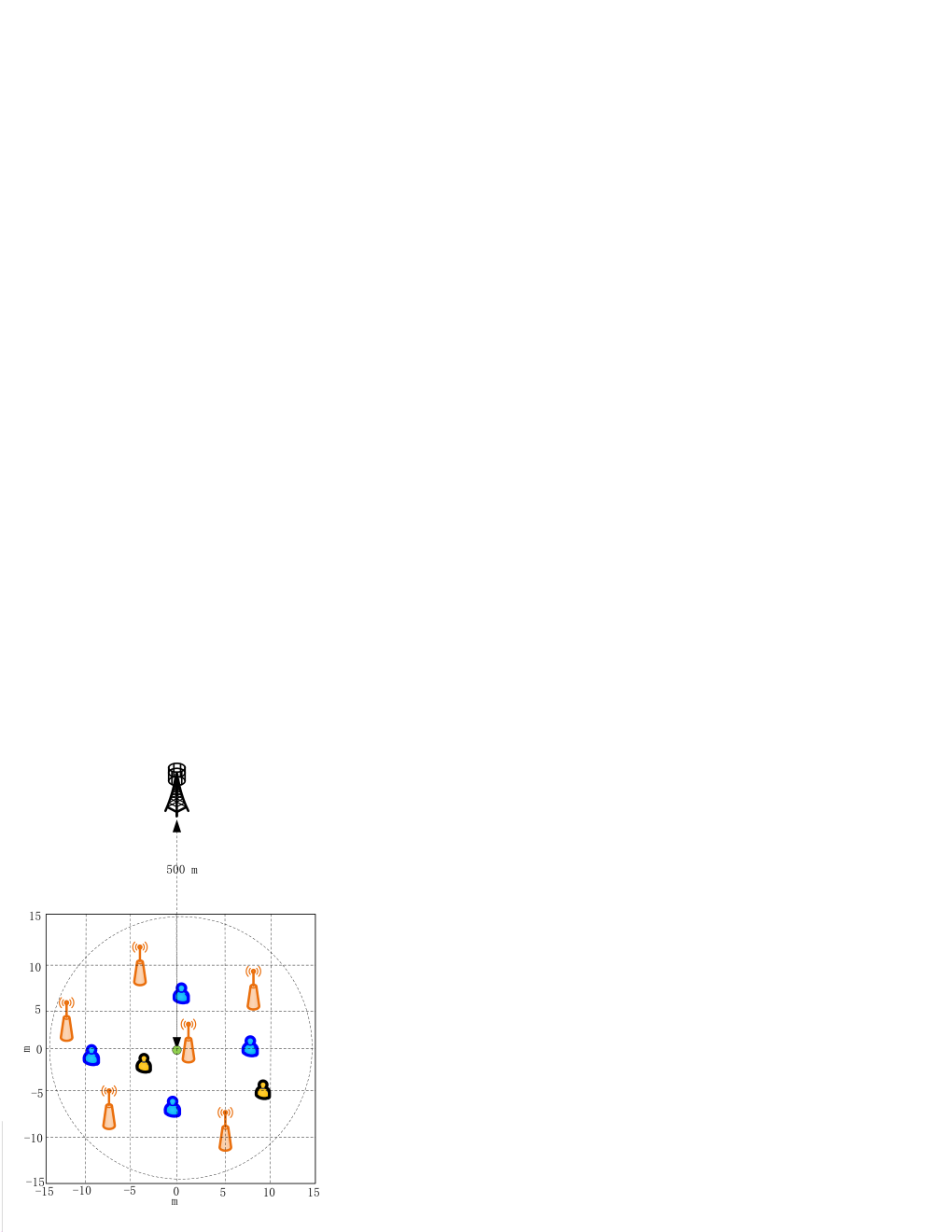
Fig. 3 demonstrates the convergence property of the different schemes, where we set dBm and dBm. For the per-BS transmit power constraint, the total BS transmit power is equally allocated to each BS. Observe that the secrecy rate converges for all schemes. Additionally, the secrecy rate under the total BS transmit power constraint is slightly higher than that under per-BS transmit power constraint. This is because the affordable transmit power of each BS is fixed and limited under the per-BS transmit power constraint. However, the power can be flexibly allocated among BSs according to the CSI so that it improves the secrecy rate under the total BS transmit power constraint. As expected, the secrecy rate decreases as the channel estimation error increases. Finally, we compare the performance under our adopted single RF chain structure to that under the fully digital structure where means that each antenna is connected to a single RF chain. Although the secrecy rate is the highest for the fully digital structure, the associated hardware cost and energy consumption are high.
Fig. 4 plots the secrecy rate versus the total BS affordable transmit power of the different schemes, and we set dBm. It can be observed that the secrecy rate first increases and then becomes saturated for all four cases. Although the secrecy rate can be increased as the total BS transmit power increases, the rate provided by the fronthaul link is limited due to the CP’s limited transmit power. Therefore, even when the access link can potentially provide higher rate, the effective secrecy rate will be limited by the fronthaul link. Additionally, one can observe that the secrecy rate under the total BS transmit power constraint is higher than that under the per-BS transmit power constraint when the affordable transmit power is low, whereas they are almost the same when the total BS affordable transmit power is high. In fact, the affordable transmit power is indeed dissipated when it is lower. However, as total BS affordable transmit power increases, it is unnecessary for each BS to dissipate all the affordable transmit power for increasing the rate, and this is because the fronthaul link does not provide a sufficiently high rate due to the CP’s limited transmit power. As a result, the secrecy rates of the two schemes are the same.
In Fig. 5, we show the secrecy rate versus the CP’s affordable transmit power, and we set dBm. We observe that the secrecy rate increases as the CP transmit power increases for all schemes. Furthermore, the secrecy rate under the total BS and per-BS transmit power constraints is the same. This is because that when and dBm, the rate provided by the fronthaul link is still lower than the rate of the access link. To characterize the access link, Fig. 6 shows the secrecy rate versus the CP’s affordable transmit power at dBm. Observe that the secrecy rate first increases and then saturates as the CP transmit power increases since the BSs cannot provide a higher rate due to their limited transmit power. In this case, the effective secrecy rate cannot be improved even when the fronthaul link can support a higher rate.
Fig. 7 shows the secrecy rate versus the number of users under four schemes, where we set dBm and dBm. Indeed, it is expected that more users result in a higher sum secrecy rate. However, the secrecy rate is reduced when the channel estimation error is increased. Meanwhile, the gap of secrecy rate between the total BS and per-BS transmit power constraints becomes smaller as the number of users increases. In fact, when a single user supported by the BS cluster is close to any one of the BSs, it will be far away from the other BSs. In this case, the other BSs must overcome the large path loss to serve this user. However, as the number of users increases, each BS may serve several users in its vicinity, hence the BSs tend to allocate more power to these “near” users for improving their secrecy rate when operating under the per-BS transmit power constraint.
Finally, in Fig. 8, we plot the secrecy rate versus the number of Eves for different schemes, where we set dBm, dBm and . As expected, the secrecy rate decreases as the number of Eves increases. Apparently, more Eves lead to higher wiretap rate, hence automatically decreasing the secrecy rate. Additionally, the secrecy rate gap between the total BS and per-BS transmit power constraints becomes smaller, as the number of Eves increases. The reason is similar to that in Fig. 7.
VII Conclusions
In this paper, we have investigated a secure BF design problem in the BS-cooperation-aided mmWave C-RAN relying on a microwave multicast fronthaul. We designed an advanced analog BF design scheme and we jointly optimized the multicast BF, digital BF and the AN covariance for maximizing the secrecy rate under the total BS and per-BS transmit power constraints. On this basis, we proposed convex approximation techniques and a CCCP-based iterative algorithm for solving them. The perfect CSI assumption of the Eves links was subsequently replaced by imperfect CSI and the worst case SRM problem was considered. Finally, an -procedure-based iterative algorithm was developed. Our results have shown that the secrecy rate is the highest under the total BS transmit power constraint, and the computational complexity of solving the above problem is also the lowest, which is quantified by . Although the secrecy rate is relatively low under the imperfect CSI assumption for the Eves links compared to the other schemes and the computational complexity of solving the formulated problem is the highest given by , the problem considered is more practical and meaningful.
Appendix A Proof of Theorem 1
It is clear that the SDP-relaxed problem (47) is jointly convex with respect to the optimization variables, and thus it satisfies Slater’s constraint qualification. Therefore, the Karush-Kuhn-Tucker (KKT) conditions are necessary and sufficient conditions for the optimal solutions of problem (47). Next, we focus our attention on the KKT conditions related to the optimal and , namely:
| (70a) | ||||
| (70b) | ||||
| (70c) | ||||
| (70d) | ||||
| (70e) | ||||
where , and , are the optimal Lagrange multipliers for the dual problem of (47).
First, we prove . Multiplying both sides of (70a) by and combing (70d), we have
| (71) |
When , the following equation must hold
| (72) |
as and thus we have
| (73) |
Next, we prove that there always exists a so that . When the optimal solutions of problem (47) are obtained, there exists at least an satisfying . We first consider a special case, namely for any , and we have
| (74) |
Let . Then can be decomposed as , , and we have
| (75) |
We define as a -by- Hermitian matrix, and formulate the following linear equation:
| (76) |
For , there are unknown real parts and unknown imaginary parts, and thus the total number of real-value variables is . Therefore, there are unknowns and equations in (76).
If , there must exist a nonzero solution for linear (76). We denote as eigenvalues of , and define
| (77) |
and it is easy to obtain the following matrix
| (78) |
Let us define , which has the following properties [49]:
- •
Rank of at least reduces one: .
- •
Primal feasibility:
- •
Power constraint: .
According to the above properties, it the clear that the feasible solution is also the optimal solution for problem (47). If we have , repeat the above procedure, else, stop. Then we have , namely .
If there are equations satisfying , we can use the above method to obtain . Therefore, there always exists a such that .
Next, we prove that if there exists any so that , we have . According to the above assumption, it is easy to obtain the following conclusions
| (79a) | ||||
| (79b) | ||||
Appendix B Proof of Theorem 2
According to (70b), when , is a positivedefinite matrix which has full rank, namely we have . Then we have
| (81) |
While according to (81), the rank of is either or . If , due to (70d), which means that the users cannot receive any signal. Thus, we have , and the null space of has a single dimension. Meanwhile, (70d) indicates that must lie in the null-space of . Therefore, it must hold , which concludes the proof.
Appendix C The Rank-One Reconstruction For
Let us introduce the notation of . In Appendix B, we assume , and . When the above assumptions do not hold, we have , which implies that is not a full-rank matrix. Then, we define as the orthogonal basis of the null space of , where , and the following must hold:
| (82) |
Let denote the th column of , where . Then, we have
| (83) |
According to (31) and the KKT condition (70), it is clear that and , and thus . As a result, we have Combining , we have . In addition, it can be shown from (70b) that . Therefore, we have However, when , we have via (70c) and (70d), and can be expressed as . However, this means that the user cannot receive the signal due to , and thus we have . Therefore, there exists only a single subspace that lies in the null space of , which is denoted as . Then, we can write . Finally, we reconstruct the new feasible as
| (84a) | ||||
| (84b) | ||||
| (84c) | ||||
Substituting into (47), we can arrive of the optimal value as the optimal solution, while satisfying all the constraints.
Appendix D The Rank-One Reconstruction For
For , the optimal BF can be directly obtained using the eigenvalue decomposition (EVD) method. Next, we adopt the randomization technique of [50] for obtaining the rank-one . First, by applying the EVD technique, we decompose as
| (85) |
We form the th candidate BF vector , where . As a result, we have . For the th candidate BF, we reformulate the following optimization problem
| (86a) | ||||
| (86b) | ||||
| (86c) | ||||
| (86d) | ||||
where
The above problem can be solved by using the method proposed in Section III. B, hence we omit the process due to the limited space. Finally, we select the optimal from all the candidate BF vectors that owns the maximum secure rate, and the optimal BF vector can be expressed as .
References
- [1] J. Li, M. Peng, Y. Yu, and Z. Ding, “Energy-efficient joint congestion control and resource optimization in heterogeneous cloud radio access networks,” IEEE Trans. Veh. Technol., vol. 65, no. 12, pp. 9873-9887, Dec. 2016.
- [2] W. Hao, O. Muta, and H. Gacanin, “Price-based resource allocation in massive MIMO H-CRANs with limited fronthaul capacity,” IEEE Trans. Wireless Commun., vol. 17, no. 11, pp. 7691-7703, Nov. 2018.
- [3] B. Dai and W. Yu, “Sparse beamforming and user-centric clustering for downlink cloud radio access network,” IEEE Access, vol. 2, pp. 1326-1339, 2014.
- [4] M. Sawahashi, Y. Kishiyama, A.Morimoto, D. Nishikawa, and M. Tanno, “Coordinated multipoint transmission/reception techniques for LTEadvanced [coordinated and distributed MIMO],” IEEE Wireless Commun., vol. 17, no. 3, pp. 26-34, Jun. 2010.
- [5] C.-L. I, J. Huang, R. Duan, C. Cui, J. X. Jiang, and L. Li, “Recent progress on C-RAN centralization and cloudification,” IEEE Access, vol. 2, pp. 1030-1039, 2014.
- [6] J. Zhang, S. Chen, R. G. Maunder, R. Zhang, and L. Hanzo, “Adaptive coding and modulation for large-scale antenna array-based aeronautical communications in the presence of co-Channel interference,” IEEE Trans. Wireless Commun., vol. 17, no. 2, pp. 1343-1357, Feb. 2018.
- [7] J. Zhang, S. Chen, R. G. Maunder, R. Zhang, and L. Hanzo, “Regularized zero-forcing precoding aided adaptive coding and modulation for large-scale antenna array based air-to-air communications,” IEEE J. Sel. Areas Commun., vol. 36, no. 9, pp. 2087–2103, Sep. 2018.
- [8] H. S. Dhillon and G. Caire, “Wireless backhaul networks: Capacity bound, scalability analysis and design guidelines,” IEEE Trans. Wireless Commun., vol. 14, no. 11, pp. 6043-6056, Nov. 2015.
- [9] B. Hu, C. Hua, J. Zhang, C. Chen, and X. Guan, “Joint fronthaul multicast beamforming and user-centric clustering in downlink C-RANs,” IEEE Trans. Wireless Commun., vol. 16, no. 8, pp. 5395-5409, Aug. 2017.
- [10] B. Dai, Y. Liu, and W. Yu, “Optimized base-station cache allocation for cloud radio access network with multicast backhaul,” IEEE J. Sel. Areas Commun., vol. 36, no. 8, pp. 1737-1750, Aug. 2018.
- [11] H. M. Wang, T. X. Zheng, and X. G. Xia, “Secure MISO wiretap channel with multi-antenna passive eavesdroppers: artificial noise vs. artificial fast fading,” IEEE Trans. Wireless Commun., vol. 14, no. 1, pp. 94-106, Jan. 2015.
- [12] W. Hao, M. Zeng, G. Sun, and P. Xiao, ”Edge cache-assisted secure low-latency millimeter wave transmission,” IEEE Internet Things J., to be published, 2019.
- [13] D. W. K. Ng, E. S. Lo, and R. Schober, “Multiobjective resource allocation for secure communication in cognitive radio networks with wireless information and power transfer,” IEEE Trans. Veh. Technol., vol. 65, no. 5, pp. 3166-3184, May 2016.
- [14] Z. Chu, K. Cumanan, Z. Ding, M. Johnston, and S. Le goff, “Robust outage secrecy rate optimizations for a MIMO secrecy channel,” IEEE Wireless Commun. Lett., vol. 4, no. 1, pp. 86-89, Feb. 2015.
- [15] J. Chen, L. Yang, and M. S. Alouini, “Physical layer security for cooperative NOMA systems,” IEEE Trans. Veh. Technol., vol. 67, no. 5, pp. 4645-4649, May 2018.
- [16] Z. Chu, K. Cumanan, Z. Ding, M. Johnston, and S. Y. Le Goff, “Secrecy rate optimizations for a MIMO secrecy channel with a cooperative jammer,” IEEE Trans. Veh. Technol., vol. 64, no. 5, pp. 1833-1847, May 2015.
- [17] L. Dai, B. Wang, M. Peng, and S. Chen, “Hybrid precoding-based millimeter-wave massive MIMO-NOMA with simultaneous wireless information and power transfer,” IEEE J. Sel. Areas Commun., vol. 37, no. 1, pp. 131-141, Jan. 2019.
- [18] Y. Ju, H. Wang, T. Zheng, Q. Yin, and M. H. Lee, “Safeguarding millimeter wave communications against randomly located eavesdroppers,” IEEE Trans. Wireless Commun., vol. 17, no. 4, pp. 2675-2689, Apr. 2018.
- [19] N. N. Alotaibi and K. A. Hamdi, “Switched phased-array transmission architecture for secure millimeter-wave wireless communication,” IEEE Trans. Commun., vol. 64, no. 3, pp. 1303-1312, Mar. 2016.
- [20] Y. Huang, J. Zhang, and M. Xiao, “Constant envelope hybrid precoding for directional millimeter-wave communications,” IEEE J. Sel. Areas Commun., vol. 36, no. 4, pp. 845-859, Apr. 2018.
- [21] Y. Zhu, L. Wang, K. Wong, and R. W. Heath, “Secure communications in millimeter wave Ad Hoc networks,” IEEE Trans. Wireless Commun., vol. 16, no. 5, pp. 3205-3217, May 2017.
- [22] X. Sun, W. Yang, Y. Cai, Z. Xiang, and X. Tang, “Secure transmissions in millimeter wave SWIPT UAV-based relay networks,” IEEE Wireless Commun. Lett., vol. 8, no. 3, pp. 785-788, Jun. 2019.
- [23] X. Sun, W. Yang, Y. Cai, L. Tao, Y. Liu, and Y. Huang, “Secure transmissions in wireless information and power transfer millimeter wave ultra-dense networks,” IEEE Trans. Inf. Forensics Security, vol. 14, no. 7, pp. 1817-1829, Jul. 2019.
- [24] S. Wang, X. Xu, K. Huang, X. Ji, Y. Chen, and L. Jin, “Artificial noise aided hybrid analog-digital beamforming for secure transmission in MIMO millimeter wave relay systems,” IEEE Access, vol. 7, pp. 28597-28606, 2019.
- [25] Y. Chen, S. He, Y. Huang, J. Ren, and L. Yang, “Robust multigroup multicast beamforming design for backhaul-limited cloud radio access network,” IEEE Signal Process. Lett., vol. 26, no. 1, pp. 189-193, Jan. 2019.
- [26] M. Tao, E. Chen, H. Zhou, and W. Yu, “Content-centric sparse multicast beamforming for cache-enabled cloud RAN,” IEEE Trans. Wireless Commun., vol. 15, no. 9, pp. 6118-6131, Sep. 2016.
- [27] Q. Vu, K. Nguyen, and M. Juntti, “Weighted max–min fairness for C-RAN multicasting under limited fronthaul constraints,” IEEE Trans. Commun., vol. 66, no. 4, pp. 1534-1548, Apr. 2018.
- [28] Y. Shi, J. Zhang, and K. B. Letaief, “Robust group sparse beamforming for multicast green cloud-RAN with imperfect CSI,” IEEE Trans. Signal Process., vol. 63, no. 17, pp. 4647-4659, Sep., 2015.
- [29] S. He, J. Ren, J. Wang, Y. Huang, Y. Zhang, W. Zhuang, and X. Shen, “Cloud-edge coordinated processing: Low-latency multicasting transmission,” IEEE J. Sel. Areas Commun., vol. 37, no. 5, pp. 1144-1158, May 2019.
- [30] Z. Yang, C. Pan, W. Xu, H. Xu, and M. Chen, “Joint time allocation and power control in multicell networks with load coupling: Energy saving and rate improvement,” IEEE Trans. Veh. Technol., vol. 66, no. 11, pp. 10470-10485, Nov. 2017.
- [31] W. Hao, M. Zeng, Z. Chu, and S. Yang, “Energy-efficient power allocation in millimeter wave massive MIMO with non-orthogonal multiple access,” IEEE Wireless Commun. Lett., vol. 6, no. 6, pp. 782-785, Dec. 2017.
- [32] B. Wang, L. Dai, Z. Wang, N. Ge, and S. Zhou, “Spectrum and energy-efficient beamspace MIMO-NOMA for millimeter-wave communications using lens antenna array,” IEEE J. Sel. Areas Commun., vol. 35, no. 10, pp. 2370-2382, Oct. 2017.
- [33] W. Zhang, J. Chen, Y. Kuo, and Y. Zhou, “Artificial-noise-aided optimal beamforming in layered physical layer security,” IEEE Commun. Lett., vol. 23, no. 1, pp. 72-75, Jan. 2019.
- [34] O. El Ayach, S. Rajagopal, S. Abu-Surra, Z. Pi, and R. Heath, “Spatially sparse precoding in millimeter wave MIMO systems,” IEEE Trans. Wireless Commun., vol. 13, no. 3, pp. 1499-1513, Mar. 2014.
- [35] X. Zhu, Z. Wang, L. Dai, and Q. Wang, “Adaptive hybrid precoding for multiuser massive MIMO,” IEEE Commun. Lett., vol. 20, no. 4, pp. 776-779, Apr. 2016.
- [36] W. Hao, Z. Chu, F. Zhou, S. Yang, G. Sun, and K. Wong, “Green communication for NOMA-based CRAN,” IEEE Internet Things J., vol. 6, no. 1, pp. 666-678, Feb. 2019.
- [37] Z. Li, M. Chen, C. Pan, N. Huang, Z. Yang, and A. Nallanathan, “Joint trajectory and communication design for secure UAV networks,” IEEE Commun. Lett., vol. 23, no. 4, pp. 636-639, Apr. 2019.
- [38] P. Song, G. Scutari, F. Facchinei, and L. Lampariello, “D3M: Distributed multi-cell multigroup multicasting,” in Proc. IEEE Int. Conf. Acoustics, Speech and Signal Processing (ICASSP), Shanghai, 2016, pp. 3741-3745.
- [39] R. Horst and N. V. Thoai, “DC programming: Overview,” J. of Optimization Theory and Application, vol. 103, no. 1, pp. 1-43, 1999.
- [40] M. Grant, S. Boyd, and Y. Ye. (2008). “CVX: Matlab software for disciplined convex programming,” [Online]. Available: http://cvxr.com/cvx/download/
- [41] Q. Zhang, Q. Li, and J. Qin, “Robust beamforming for nonorthogonal multiple-access systems in MISO channels,” IEEE Trans. Veh. Technol., vol. 65, no. 12, pp. 10231-10236, Dec. 2016.
- [42] Z. Yang, C. Pan, W. Xu, Y. Pan, M. Chen, and M. Elkashlan, “Power control for multi-Cell networks with non-orthogonal multiple access,” IEEE Trans. Wireless Commun., vol. 17, no. 2, pp. 927-942, Feb. 2018.
- [43] K.-Y. Wang, A.-C. So, T.-H. Chang, W.-K. Ma, and C.-Y. Chi, “Outage constrained robust transmit optimization for multiuser MISO downlinks: Tractable approximations by conic optimization,” IEEE Trans. Signal Process., vol. 62, no. 21, pp. 5690-5705, Nov. 2014.
- [44] J. Huang and A. L. Swindlehurst, “Robust secure transmission in MISO channels based on worst-case optimization,” IEEE Trans. Signal Process., vol. 60, no. 4, pp. 1696–1707, Apr. 2012.
- [45] Q. Li and W. Ma, “Spatially selective artificial-noise aided transmit optimization for MISO multi-eves secrecy rate maximization,” IEEE Trans. Signal Process., vol. 61, no. 10, pp. 2704-2717, May, 2013.
- [46] F. Zhou, Z. Li, J. Cheng, Q. Li, and J. Si, “Robust AN-aided beamforming and power splitting design for secure MISO cognitive radio with SWIPT,” IEEE Trans. Wireless Commun., vol. 16, no. 4, pp. 2450-2464, Apr. 2017.
- [47] T. S. Rappaport, G. R. MacCartney, M. K. Samimi, and S. Sun, “Wideband millimeter-wave propagation measurements and channel models for future wireless communication system design,” IEEE Trans. Commun., vol. 63, no. 9, pp. 3029-3056, Sep. 2015.
- [48] Evolved Universal Terrestrial Radio Access (E-UTRA); Radio Frequency (RF) requirements for LTE Pico Node B (Release 12), 3GPP Std. 36.931, 2014.
- [49] Y. Huang and D. P. Palomar, “Rank-constrained separable semidefinite programming with applications to optimal beamforming,” IEEE Trans. Signal Process., vol. 58, no. 2, pp. 664-678, Feb. 2010.
- [50] N. D. Sidiropoulos, T. N. Davidson, and Z.-Q. Luo, “Transmit beamforming for physical-layer multicasting,” IEEE Trans. Signal Process., vol. 54, no. 6, pp. 2239-2251, Jun. 2006.