1Introduction

Momentum Improves Optimization on Riemannian Manifolds

Foivos Alimisis Antonio Orvieto Gary Bécigneul Aurelien Lucchi

IST Austria ETH Zürich Gematria Technologies London, U.K. ETH Zürich

Abstract

We develop a new Riemannian descent algorithm that relies on momentum to improve over existing first-order methods for geodesically convex optimization. In contrast, accelerated convergence rates proved in prior work have only been shown to hold for geodesically strongly-convex objective functions. We further extend our algorithm to geodesically weakly-quasi-convex objectives. Our proofs of convergence rely on a novel estimate sequence that illustrates the dependency of the convergence rate on the curvature of the manifold. We validate our theoretical results empirically on several optimization problems defined on the sphere and on the manifold of positive definite matrices.

1 Introduction

The field of optimization plays a central role in machine learning. At its core lies the problem of finding a minimum of a function $f:H\rightarrow{\mathbb{R}}$ . In the vast majority of applications in machine learning, $H$ is considered to be a Euclidean vector space. However, a number of machine learning tasks can profit from a specialized problem-dependent Riemannian structure (Bonnabel 2013; Zhang and Sra 2016), which will be the focus of our discussion in this paper. Among the most popular types of methods to optimize $f$ are first-order methods, such as gradient descent that simply updates a sequence of iterates $\{x_{k}\}$ by stepping in the opposite direction of the gradient $\nabla f(x_{k})$ . In the case $H=\mathbb{R}^{n}$ , gradient descent as a first-order method has been shown to achieve a suboptimal convergence rate on convex problems ( $\mathcal{O}(1/k)$ ). In a seminal paper, (Nesterov 1983), Nesterov showed that one can construct an optimal — i.e. accelerated — algorithm that achieves faster rates of convergence for both convex ( $\mathcal{O}(1/k^{2})$ ) and strongly-convex functions. The convergence analysis of this algorithm relies heavily on the linear structure of $H$ and it is not until recently that a first adaptation to Riemannian manifolds was derived by Zhang and Sra 2018. The algorithm by Zhang and Sra 2018 is shown to obtain an accelerated rate of convergence for functions that are known to be geodesically strongly-convex, provided that one initializes in a neighborhood of the (unique) solution. These functions are of particular interest as they might be non-convex in the Euclidean sense and they occur in some relevant computational tasks, such as the approximation of the Karcher mean of positive definite matrices (Zhang et al. 2016). However, many other interesting problems belong to the weaker class of geodesically convex functions. This includes problems defined on the cone of Hermitian positive definite matrices (Sra and Hosseini 2015), which appear in various areas of machine learning such as tracking (Cheng and Vemuri 2013) and medical imaging (Zhu et al. 2007). In this paper, we therefore address the question of whether an algorithm that relies on momentum can provably achieve a faster rate of convergence for functions that are geodesically convex but not necessarily strongly convex. We also consider the extension to the weaker class of geodesically weakly-quasi-convex objective functions. A more thorough motivation for investigating convex and weakly-quasi convex objectives in Riemannian optimization can be found in Section 4 of (Alimisis et al. 2019). Our main contributions are:

1.

We propose a new practical Riemannian algorithm that exploits momentum to speed up convergence for geodesically convex and weakly-quasi-convex functions. As in (Nesterov et al. 2018), our approach uses a small-dimensional relaxation (sDR) oracle (which can be solved approximately and in linear time) to perform adaptive linear coupling¹¹ 1 See discussion in the next section. (Allen-Zhu and Orecchia 2014). In order to provide theoretical guarantees for this new algorithm, we use a novel estimate sequence combining ideas from (Nesterov et al. 2018) and (Zhang and Sra 2018) as well as develop some new results at the intersection of optimization and Riemannian geometry.
2.

Our main algorithm applied to geodesically convex objective functions provides better theoretical guarantees of convergence compared to Riemannian Gradient Descent (RGD) (Zhang and Sra 2016), given that the bound on the working domain is not exceedingly large. Since RGD is the only known first-order method with guaranteed convergence for geodesically convex functions, our algorithm has the best known worst-case behaviour. Moreover, our algorithm is accelerated for the first (practically large) part of the optimization procedure.
3.

We validate our theoretical findings numerically on several important machine learning problems defined on manifolds of both positive curvature (Rayleigh quotient maximization) and negative curvature (operator scaling and Karcher mean approximation). Some of these problems are convex (but not strongly-convex) while others have a relatively small strong convexity constant. We show the empirical superiority of our method when compared to Riemannian algorithms designed for well-conditioned geodesically strongly-convex objectives, such as RAGD (Zhang and Sra 2018).

2 Related Work

Accelerated Gradient Descent (AGD).

The first accelerated gradient descent algorithm in Euclidean vector spaces is due to Nesterov 1983. Since then, the community has shown a deep interest in understanding the mechanism underlying acceleration. A recent trend has been to look at acceleration from a continuous-time viewpoint (Su et al. 2014; Wibisono et al. 2016). In this framework, AGD is seen as the discretization of a second-order ODE. Alternatively, Allen-Zhu and Orecchia 2014 showed how one can view AGD as a primal-dual method performing linear coupling between gradient descent and mirror descent. Recently Nesterov et al. 2018 proposed AGDsDR, a modification of the method by Allen-Zhu and Orecchia 2014, which adaptively selects the linear coupling parameter (denoted by $\beta$ ) at each iteration using an approximate line search. This work will serve as an inspiration for us to design an accelerated Riemannian algorithm.

Riemannian optimization.

Research in the field of Riemannian optimization has encountered a lot of interest in the last decade. A seminal book in the area is (Absil et al. 2009), which gives a comprehensive review of many standard optimization methods, but does not discuss acceleration. More recently, Zhang and Sra 2016 proved convergence rates for Riemannian gradient descent applied to geodesically convex functions. Acceleration in a Riemannian framework was first discussed by Liu et al. 2017, who claimed to have designed a Riemannian method with guaranteed acceleration. While their methodology is interesting, unfortunately, as discussed in (Zhang and Sra 2018), their algorithm relies on finding the exact solution to a nonlinear equation at each iteration, and it is not clear how difficult this additional problem might be or how approximation errors accumulate. Subsequently, Zhang and Sra 2018 developed the first computationally tractable accelerated algorithm on a Riemannian manifold, but their approach only has provable convergence for geodesically strongly-convex objectives (provided that one initializes sufficiently close to the solution). A more recent work, (Ahn and Sra 2020), attempts to tackle the problem of acceleration for geodesically strongly-convex optimization with global convergence rate (no assumptions on the initialization required). Notwithstanding the theoretical significance of this work, the final algorithm has the practical drawback that achieves full acceleration only in late training (after a possibly very large number of steps for ill-conditioned problems), while at the beginning behaves comparably to Riemannian gradient descent. Instead, using a continuous-time viewpoint, the recent work (Alimisis et al. 2019) analyzed various ODEs that can model acceleration on Riemannian manifolds with theoretical guarantees of convergence. They derived discrete-time algorithms via numerical integration of the continuous-time process but do not provide theoretical guarantees for the discrete-time schemes. The problem we address is different from prior work as we aim to demonstrate that momentum provably yields a better rate of convergence than Riemannian gradient descent for the classes of geodesically convex and weakly-quasi-convex functions, which are both of significant practical interest (see discussion in Section 6). We note that extending the proof by Zhang and Sra 2018 to these weaker classes of functions is not straightforward due to some distortions between the tangent spaces of the sequence of iterates of the algorithm ²² 2 By ”distortion”, we mean that when considering two successive iterates $x_{k}$ and $x_{k+1}$ , the terms $\log_{x_{k}}(a)-\log_{x_{k}}(b)$ and $\log_{x_{k+1}}(a)-\log_{x_{k+1}}(b)$ appearing in the estimate sequence belong to different tangent spaces and are therefore not directly comparable (while they are exactly the same in the Euclidean case).. Indeed, the estimate sequence used in (Zhang and Sra 2018) relies on changing the tangent space at each step. These successive changes give rise to additional errors which can be dealt with by relying on the strong convexity assumption. However, we were unable to adapt their proof to weaker function classes. Instead, we rely on a novel estimate sequence that is qualitatively different from the one used in (Zhang and Sra 2018) in order to avoid distortions produced by changing tangent spaces.

3 Background

3.1 Preliminaries from Differential Geometry

We review some basic notions from Riemannian geometry that are required in our analysis. For a full review, we refer the reader to some classical textbook, for instance (Spivak 1979).

Manifolds.

A differentiable manifold $M$ is a topological space that is locally Euclidean. This means that for any point $x\in M$ , we can find a neighborhood that is diffeomorphic to an open subset of some Euclidean space. This Euclidean space can be proved to have the same dimension, regardless of the chosen point, called the dimension of the manifold.
A Riemannian manifold $(M,g)$ is a differentiable manifold equipped with a Riemannian metric $g_{x}$ , i.e. an inner product for each tangent space $T_{x}M$ at $x\in M$ . We denote the inner product of $u,v\in T_{x}M$ with $\langle u,v\rangle_{x}$ or just $\langle u,v\rangle$ when the tangent space is obvious from context. Similarly we consider the norm as the one induced by the inner product at each tangent space. The Riemannian metric provides us a way to measure the distance $d$ between points on the manifold, transforming it into a metric space. Given $A\subseteq M$ , the diameter of $A$ is defined as $\textnormal{diam}(A)=\sup_{p,q\in A}d(p,q)$ .

Geodesics.

Geodesics are curves $\gamma:[0,1]\rightarrow M$ of constant speed and of (locally) minimum length. They can be thought of as the Riemannian generalization of straight lines in Euclidean space. Geodesics are used to construct the exponential map $\exp_{x}:T_{x}M\rightarrow M$ , defined by $\exp_{x}(v)=\gamma(1)$ , where $\gamma$ is the unique geodesic such that $\gamma(0)=x$ and $\dot{\gamma}(0)=v$ . The exponential map is locally a diffeomorphism. We denote the inverse of the exponential map $\exp_{x}$ (in a neighborhood $U\subseteq M$ of $x$ ) by $\log_{x}:U\to T_{x}M$ . Geodesics also provide a way to transport vectors from one tangent space to another. This operation, called parallel transport, is usually denoted by $\Gamma_{x}^{y}:T_{x}M\rightarrow T_{y}M$ .

Vector fields and covariant derivative.

The correct notion to capture second order changes on a Riemannian manifold is called covariant differentiation and it is induced by the fundamental property of Riemannian manifolds to be equipped with a connection. We are interested in a specific type of connection, called the Levi-Civita connection, which induces a specific type of covariant derivative. The fact that a unique Levi-Civita connection exists always in a Riemannian manifold is the subject of the fundamental theorem of Riemannian geometry. However, for the purpose of our analysis, it will be sufficient to rely on a simple notion of covariant derivative that relies on the (more visualizable) notion of parallel transport. First, we define vector fields on a Riemannian manifold as sections of the tangent bundle.

Definition 1.

Let $M$ be a Riemannian manifold. A vector field $X$ in $M$ is a smooth map $X:M\rightarrow\mathcal{T}M$ , where $\mathcal{T}M$ is the tangent bundle, i.e. the collection of all tangent vectors in all tangent spaces of $M$ , such that $p\circ X$ is the identity ( $p$ projects from $\mathcal{T}M$ to $M$ ).

One can see a vector field as an infinite collection of imaginary curves, the so-called integral curves (formally solutions of first order differential equations on $M$ ).

Definition 2.

Given two vector fields $X,Y$ in a Riemannian manifold $M$ , we define the covariant derivative of $Y$ along $X$ to be $\nabla_{X}Y(p)=\lim_{h\to 0}\frac{\Gamma_{\gamma(h)}^{p}Y(\gamma(h))-Y(p)}{h}$ , where $\gamma$ is the unique integral curve of $X$ , starting from $p$ , i.e $\gamma(0)=p$ .

3.2 Geodesic convexity

We remind the reader of the basic definitions needed in Riemannian optimization.

Definition 3.

A subset $A\subseteq M$ of a Riemannian manifold $M$ is called geodesically uniquely convex, if every two points in $A$ are connected by a unique geodesic.

Definition 4.

A function $f:A\rightarrow{\mathbb{R}}$ is called geodesically convex, if for any $p,q\in M$ , we have $f(\gamma(t))\leq(1-t)f(p)+tf(q)$ for any $t\in[0,1]$ , where $\gamma$ is the geodesic connecting $p,q\in M$ .

Given a function $f:M\rightarrow{\mathbb{R}}$ , the notions of differential and (Riemannian) inner product allow us to define the Riemannian gradient of $f$ at $x\in M$ , which is a tangent vector belonging to the tangent space based at $x$ , $T_{x}M$ .

Definition 5.

The Riemannian gradient gradf of a (real-valued) function $f:M\rightarrow{\mathbb{R}}$ at a point $x\in M$ , is the tangent vector at $x$ , such that $\langle\textnormal{{gradf}}(x),u\rangle=df(x)u$ ³³ 3 $df$ denotes the differential of $f$ , i.e. $df(x)[u]=\lim_{t\to 0}\frac{f(c(t))-f(x)}{t},$ where $c:I\to M$ is a smooth curve such that $c(0)=x$ and $\dot{c}(0)=u$ ., for any $u\in T_{x}M$ .

Given the notion of Riemannian gradient and covariant derivative we define the notion of Riemannian Hessian.

Definition 6.

The Hessian of $f$ is defined as a bilinear form at each point $p\in M$ , given by $\operatorname{Hess}_{p}(f)(X,Y)=\langle\nabla_{X}\operatorname{grad}f,Y\ \rangle$ , for two vector fields $X,Y$ on $M$ .

Using the Riemannian inner product and gradient, we can formulate an equivalent definition for geodesic convexity for a smooth function $f$ defined in a geodesically uniquely convex domain $A$ .

Proposition 1.

Let $f:A\rightarrow{\mathbb{R}}$ be a smooth, geodesically convex function. Then, for any $x,y\in A$ ,

\displaystyle f(y)-f(x)\geq\langle\textnormal{{gradf}}(x),\textnormal{{log}}_{x}(y)\rangle.

As in the Euclidean case, any local minimum of a geodesically convex function is a global minimum. We now generalize the well-known notion of Euclidean weak-quasi-convexity to Riemannian manifolds. For a review of this notion, we refer the reader to (Guminov and Gasnikov 2017).

Definition 7.

A function $f:A\rightarrow{\mathbb{R}}$ is called geodesically $\alpha$ -weakly-quasi-convex with respect to $c\in M$ , if $\alpha(f(c)-f(x))\geq\langle\textnormal{gradf}(x),\textnormal{log}_{x}(c)\rangle$ for some fixed $\alpha\in(0,1]$ and any $x\in A$ .

It is easy to see that weak-quasi-convexity implies that any local minimum of $f$ is also a global minimum. Using the notion of parallel transport we can define when $f$ is geodesically $L$ -smooth, i.e. has Lipschitz continuous gradient in a differential-geometric way.

Definition 8.

$f:A\rightarrow{\mathbb{R}}$ is called L-smooth if $\|\textnormal{gradf}(x)-\Gamma_{y}^{x}{\textnormal{gradf}(y)}\|\leq L\|\textnormal{log}_{x}(y)\|$ for any $x,y\in A$ .

Geodesic $L$ -smoothness has similar properties to its Euclidean analogue: a two times differentiable function is $L$ -smooth, if and only if the norm of its Riemannian Hessian is upper bounded by $L$ .

3.3 Basic Assumptions

In this paper, we make the standard assumption that the input space is not "infinitely curved". In order to make this statement rigorous, we need the notion of sectional curvature $K$ , which is a measure of how sharply the manifold is curved (or how “far” from being flat our manifold is), “two-dimensionally”. More concretely, as in (Zhang and Sra 2018), we make the following set of assumptions:

Assumption 1.

Given $A\subseteq M$ geodesically uniquely convex, and $f:A\to{\mathbb{R}}$ ,

1.

The sectional curvature $K$ inside $A$ is bounded from above and below, i.e. $K_{min}\leq K\leq K_{\max}$ .
2.

$A$ is a geodesically uniquely convex subset of $M$ , such that $\textnormal{diam}(A)\leq D<\infty$ . This implies that the exponential map $\exp_{x}:T_{x}M\rightarrow M$ is globally a diffeomorphism for any $x\in A$ with inverse denoted by $\log_{x}$ .
3.

$f$ is geodesically $L$ -smooth with its local minima (which are all global) inside $A$ , we denote some of them by $x^{*}$ .
4.

We have granted access to oracles which compute the exponential and logarithmic maps as well as the Riemannian gradient of $f$ efficiently.
5.

All the iterates of our algorithms remain inside $A$ .

The last assumption is standard in accelerated Riemannian optimization, (Zhang and Sra 2018; Alimisis et al. 2019; Ahn and Sra 2020), and we did not observe it to be violated in our experiments. However, it remains an open question as to whether it could be relaxed or even removed completely from our analysis.

4 The RAGDsDR Algorithm

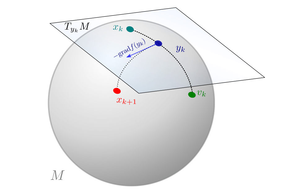
We now develop a new Riemannian algorithm that relies on momentum and which is inspired by the Euclidean algorithm presented in (Nesterov et al. 2018) (see description in Appendix A). It is detailed in Algorithm 1 and illustrated in Figure 1. At each iteration $k$ , the next iterate $x_{k+1}$ (line 5) is computed by taking a gradient step at an interpolated point $y_{k}$ (line 4) which follows the direction of a momentum term $\log_{v_{k}}(x_{k})$ . The main difference with the Euclidean case is that the curve from $v_{k}$ to $x_{k}$ is a geodesic on the manifold $M$ instead of a straight Euclidean line. As in (Nesterov et al. 2018), we also rely on a minimization over a closed interval (i.e. the small-dimension relaxation, sDR) to choose the best possible stepsize $\beta_{k}$ (line 3) on the geodesic connecting $v_{k}$ to $x_{k}$ . We will see in the next section that this minimization is computationally fast to solve (also see Section 6), can be computed approximately and practically yields faster convergence than the typical fixed parameter $\beta_{k}=\frac{k}{k+2}$ (Nesterov 2018). The curvature of $M$ is involved directly in the algorithm via the quantity $\zeta\geq 1$ (line 6), defined as

\zeta:=\begin{cases}\sqrt{-K_{\min}}D\coth(\sqrt{-K_{\min}}D)&,K_{\min}<0\\ 1&,K_{\min}\geq 0\end{cases}

(1)

Algorithm 1 RAGDsDR for convex functions

A_{0}=0,x_{0}=v_{0}\in A

2: for

k\geq 0

\beta_{k}=\underset{\beta\in[0,1]}{\mathrm{argmin}}\left\{f(\exp_{v_{k}}(\beta\log_{v_{k}}(x_{k})))\right\}

y_{k}=\exp_{v_{k}}(\beta_{k}\log_{v_{k}}(x_{k}))

x_{k+1}=\exp_{y_{k}}\left(-\frac{1}{L}\text{grad}f(y_{k})\right)

\frac{\zeta a_{k+1}^{2}}{A_{k}+a_{k+1}}=\frac{1}{L},a_{k+1}>0

A_{k+1}=A_{k}+a_{k+1}

v_{k+1}=\exp_{v_{k}}\left(-a_{k+1}\Gamma_{y_{k}}^{v_{k}}\text{grad}f(y_{k})\right)

9: end for

Refer to caption — Figure 1: Illustration of one step of Algorithm 1. The point $y_{k}$ is computed to minimize $f$ on the geodesic between $x_{k}$ and $v_{k}$ . $x_{k+1}$ is computed by taking a gradient step from $y_{k}$ and projected using the exponential map $\exp_{y_{k}}(\cdot)$ .

The discriminant of the quadratic equation defining $a_{k+1}$ at step 6 is positive, thus the aforementioned equation has a positive and negative solution, from which we choose the first.

The computation of the parallel transport at step 8 is given directly by the oracle, since it relies on the computation of the exponential map. For manifolds found in applications, the parallel transport is cheap and implementations are found in libraries such as (Townsend et al. 2016).

The definition of $v_{k+1}$ at step 8 is qualitatively different from the one in (Zhang and Sra 2018), but not heavier computationally, since in both cases we need three oracle calls. Note that Nesterov et al. 2018 define $v_{k+1}$ through a minimization problem (see Appendix A). This approach could be naively generalized to the Riemannian setting but it would yield a minimization problem that has no explicit solution due to non-linearity. Instead, we find a generalization of the Euclidean definition that can be solved explicitly and write $v_{k+1}$ directly in its explicit form in Algorithm 1.

Geodesic search.

The second step in Algorithm 1 is solved using a procedure similar to a line search which we name geodesic search. It guarantees that the following two key conditions hold (proof in App. B):

\displaystyle f(y_{k})\leq f(x_{k})\text{ and }\langle\text{grad}f(y_{k}),\log_{y_{k}}(v_{k})\rangle\geq 0.

(2)

Practically, the geodesic search procedure is inexact. While we can still expect the first inequality in Eq. 2 to be satisfied exactly, the second one can only be satisfied up to a small error $\tilde{\epsilon}>0$ , i.e. $\langle\text{grad}f(y_{k}),\log_{y_{k}}(v_{k})\rangle\geq-\tilde{\epsilon}$ . We note that this is an analogous condition to the one used by Nesterov et al. 2018 in the Euclidean case. As we will see shortly, one of the main quantities of interest in our analysis will be

\mathcal{E}_{k}(x):=\langle\text{grad}f(y_{k}),\log_{y_{k}}(x)-\Gamma_{v_{k}}^{y_{k}}\log_{v_{k}}(x)\rangle,

(3)

which occurs as an error in our estimate-sequence analysis and captures the curved nature of the manifold $M$ . We will prove that the absolute value of this error is bounded by the sum of two terms, namely $\mid\mathcal{E}_{k}(x)\mid\leq\tilde{\epsilon}+\tilde{\eta}_{k}$ , where $\tilde{\epsilon}$ is the error obtained by the geodesic search and $\tilde{\eta}_{k}$ is an extra curvature-dependent error. The latter depends on an upper bound on the working domain $D$ and it decays to $0$ as the algorithm runs. In the Euclidean case $\tilde{\eta}_{k}=0$ . We will prove that in the Riemannian case $\tilde{\eta}_{k}=\mathcal{O}\left(\frac{d(M)}{k}\right)$ , where $d(M)$ is a small constant which depends on the sectional curvature and a bound of our working domain.

5 Convergence Analysis

Geodesically-convex functions.

We now present our main convergence result.

Our analysis is based on a novel estimate sequence, which allows for an extra error at each step. However, this extra error does not accumulate, and it decays linearly over iterations. As a result, we obtain a rate of convergence that is superior to the convergence guarantees of RGD derived in (Zhang and Sra 2016) under a restriction on the bound of the working domain (see later discussion).
We first need to examine the behaviour of $\mathcal{E}_{k}(x)$ :

Lemma 2.

Under our set of assumptions (Assumption 1), Algorithm 1 produces iterates $y_{k},v_{k}$ such that

-\mathcal{E}_{k}(x)\leq\|\text{grad}f(y_{k})\|\max\{\zeta-1,1-\delta\}D+\tilde{\epsilon}

with $\zeta\geq 1$ defined by equation (1) and $\delta\leq 1$ defined by

\delta:=\begin{cases}1&,K_{\max}\leq 0\\ \sqrt{K_{\max}}D\cot(\sqrt{K_{\max}}D)&,K_{\max}>0\end{cases}

We prove this lemma in Appendix C. We rely on various geometric bounds derived in Appendix D, which are inspired by those of Alimisis et al. 2019. Generally speaking, $\delta$ and $\zeta$ are obtained by considering the spectral properties of an operator similar to the Riemannian Hessian of the squared distance function, $\delta$ as a lower bound of its smallest eigenvalue and $\zeta$ as an upper bound of the largest one.

We are now ready to state our main convergence result:

Recall that parameter $D$ is used to denote an upper bound for the diameter of our working domain (Assumption 1).

The proof is derived in Appendix E and relies on Lemma 2. At first glance, the upper bound seems rather intuitive for those familiar with Riemannian optimization, namely the positive-curvature case provides the same guarantees as the Euclidean one, while the negative-curvature case provides worse guarantees.
Let’s take a closer look at the rate of convergence. To do so, we define the following quantity which we call the “discrepancy” of the manifold $M$ .

Definition 9.

The discrepancy of the manifold $M$ is defined as $d(M):=4\max\{\zeta-1,1-\delta\}$ .

In the Euclidean case, we have $d(M)=0$ , thus our algorithm is a generalization of accelerated gradient descent with line search.
The convergence rate in Thm. 3 is accelerated when

\frac{2\zeta LD^{2}}{k^{2}}\geq d(M)\frac{\zeta LD^{2}}{k}

which is equivalent to $k\leq\cfrac{2}{d(M)}.$ Thus, $2/d(M)$ is an upper bound indicating how many steps of the algorithm can be performed with an accelerated convergence rate. When the manifold $M$ tends to be Euclidean in the sense that $\max\{\mid K_{min}\mid,\mid K_{max}\mid\}\rightarrow 0$ , then $d(M)\rightarrow 0$ and $\frac{2}{d(M)}\rightarrow\infty$ , increasing the numbers of iterations that one can perform accelerated optimization.
Even when we exceed this bound, the condition

2d(M)<\frac{1}{2}\Leftrightarrow\max\{\zeta-1,1-\delta\}<\frac{1}{16}

(4)

suffices to guarantee a better worst-case upper bound than Riemannian Gradient Descent in (Zhang and Sra 2016) (Theorem 13), since we have a smaller constant in the numerator. This is because the rate provided in Theorem 13 in (Zhang and Sra 2016) is

f(x_{k})-f^{*}\leq\frac{\zeta LD^{2}}{2(\zeta+k-2)}

Condition (4) implies that $\frac{\zeta LD^{2}}{2(\zeta+k-2)}>2d(M)\frac{\zeta LD^{2}}{k}$ , since $4d(M)<1$ and $\zeta<2$ (which implies that
$\frac{1}{k}<\frac{1}{\zeta+k-2}$ ).

Finally, condition (4) is for instance satisfied if

\sqrt{\mid K_{min}\mid}D\leq 0.4,\quad\text{and}\quad\sqrt{\mid K_{max}\mid}D\leq 0.4.

Both conditions hold if and only if the curvature of the manifold is in absolute value less or equal than $\frac{0.16}{D^{2}}$ . We summarize these facts in the following theorem:

In practical situations, we have observed that the quantity $d(M)$ is very small, and we therefore empirically observe acceleration for a very large number of iterations (almost until convergence). We refer the reader to the discussion in Section 7 which also includes a comparison with (Zhang and Sra 2018).

Geodesically weakly-quasi-convex functions.

We extend Algorithm 1 to functions that are $\alpha$ -weakly-quasi-convex. This requires to restart Algorithm 1 whenever the suboptimality at the current iteration is less than the previous one by a factor $1-\frac{\alpha}{c}$ , where $c>1$ is a constant. This procedure yields Alg. 2.

Algorithm 2 RAGDsDR for weakly-quasi-convex functions

1: for

i\geq 0

A_{0}=0,x_{0}^{i}=v_{0}^{i}\in A

3: for

k\geq 0

\beta_{k}=

\argmin_{\beta\in[0,1]}\left\{f\left(\exp_{v_{k}^{i}}\left(\beta\log_{v_{k}^{i}}(x_{k}^{i})\right)\right)\right\}

y_{k}^{i}=\exp_{v_{k}^{i}}\left(\beta_{k}\log_{v_{k}^{i}}(x_{k}^{i})\right)

x_{k+1}^{i}=\exp_{y_{k}^{i}}\left(-\frac{1}{L}\text{grad}f(y_{k}^{i})\right)

\frac{\zeta a_{k+1}^{2}}{A_{k}+a_{k+1}}=\frac{1}{L},a_{k+1}>0

A_{k+1}=A_{k}+a_{k+1}

v_{k+1}^{i}=\exp_{v_{k}^{i}}\left(-a_{k+1}\Gamma_{y_{k}^{i}}^{v_{k}^{i}}\text{grad}f(y_{k}^{i})\right)

10: if

f(x_{k}^{i})-f(x^{*})\leq\left(1-\frac{\alpha}{c}\right)(f(x_{0}^{i})-f(x^{*}))

then

11: break

12: end if

13: end for

14:

x_{0}^{i+1}=x_{N}^{i}

(where

N

is the number of steps performed in the loop over

k

)

15: end for

As in the convex case, the $\mathcal{O}(\frac{1}{N})$ part of the rate is multiplied by the discrepancy of the manifold $d(M)$ , thus the analysis of Theorem 4 holds almost the same. The proof can be found in Appendix F.

6 Numerical Experiments

We validate our findings on Riemannian manifolds of both positive and negative curvature. Our code⁴⁴ 4 https://github.com/aorvieto/RAGDsDR is built on top of PyManopt (Townsend et al. 2016). We compare RAGDsDR (Algorithm 1) with Riemannian Gradient Descent (RGD) and, when possible (i.e. when we can estimate the strong convexity modulus), with RAGD by Zhang and Sra 2018. As a more practical alternative to the geodesic search in step 2 (which we solve with at most 10 iterations of golden-section search), we show the performance for $\beta_{k}=\frac{k}{k+2}$ . Under this choice, RAGDsDR recovers a Riemannian version of Linear Coupling (Allen-Zhu and Orecchia 2014).

6.1 Positive curvature

We first consider the problem of maximizing the Rayleigh quotient $\frac{x^{T}Ax}{2\|x\|_{2}^{2}}$ over ${\mathbb{R}}^{d}$ , i.e. of finding the dominant eigenvector of $A\in{\mathbb{R}}^{d\times d}$ . This non-convex problem can be written on the open hemisphere $\mathbb{S}^{d-1}$ (constant positive curvature) : $\argmin_{x\in\mathbb{S}^{d-1}}f(x):=-\frac{1}{2}x^{T}Ax.$ It is well known that, in the Euclidean case, such an objective is hard to optimize if $A$ is high-dimensional and ill-conditioned --- and is therefore able to truly showcase the acceleration phenomenon⁵⁵ 5 Indeed, high dimensional quadratics are used to construct lower bounds in (Nesterov 1983). for convex but not necessarily strongly-convex functions, in a tight way. We choose $A=\frac{1}{d}BB^{T}$ , where $B\in{\mathbb{R}}^{d\times n}$ has standard Gaussian entries⁶⁶ 6 Inspired by PCA and linear regression, where $B$ is the design matrix ( $n$ data points).. We choose $d=2000$ and $n=2100\approxeq d$ , leading to a large condition number. In correspondence to the Euclidean case, we have $L=\lambda_{\text{max}}(A)$ and use a step-size of $1/L$ for RGD and RAGD. Also, we choose the strong-convexity modulus $\mu$ (needed parameter for RAGD) as $\lambda_{\text{min}}(A)$ , again in correspondence with the Euclidean case.

Results.

As predicted by Theorem 3, Figure 2 shows that RAGDsDR is able to accelerate RGD from $\mathcal{O}(1/k)$ to $\mathcal{O}(1/k^{2})$ during the first hundred iterations. The rate will eventually⁷⁷ 7 This happens quite late, around iteration $k=100$ , because of the large condition number $\kappa(A)\approxeq 4000$ . become linear, due to the gradient-dominance of $f$ (Thm. 4 in (Zhang et al. 2016)). In contrast, RAGD is only able to profit from acceleration at a late stage — before that, it is comparable to RGD.
We note that the choice $\beta_{k}=\frac{k}{k+2}$ , which reduces the iteration-cost of RAGDsDR, does not influence much the empirical rate. Indeed, as shown in the figure, the geodesic search returns a result which is somehow similar. However, as also mentioned in (Nesterov et al. 2018), the geodesic search increases the adaptiveness of the method to curvature, providing better stability (no oscillations) and steady decrease at each iteration.

Comment on regularization.

In the Euclidean setting, one can sometimes add a quadratic regularizer to accelerate the convergence of momentum methods designed for strongly-convex objectives. For the Rayleigh quotient problem, one may replace $A$ with $A+\gamma I_{d\times d}$ , where $\gamma>0$ . We note that there is typically no general principle for choosing an appropriate $\gamma$ (which is tie to generalization in machine learning). However, such a regularization technique increases the value of the strong-convexity modulus $\mu$ , which speeds up optimizers designed for strongly-convex problems. Instead, the algorithm we present in this paper provably improves over RGD in terms of gradient computations, and this effect is independent of $\mu$ . To the best of our knowledge, RAGDsDR is the only Riemannian algorithm in the current literature with these features. To conclude, we also note that the derivation of accelerated rates for problems which are not strongly-convex has a long history in convex optimization (e.g. Nesterov’s 1983 seminal paper (Nesterov 1983)) and arguably deserves the same attention in Riemannian optimization.

Comment on the wall-clock time performance.

RAGDsDR, with or without geodesic search, only requires the computation of one gradient per iteration. However, the calculation of $\beta_{k}$ using geodesic search (line 3 in Algorithm 1) increases the time complexity. The approximation of $\beta_{k}$ does not require additional gradients, but just a few (in this case 8 per iteration) function evaluations. For simple problems such as the ones we present in this section, the overall complexity is dominated by the call of geometric operations like the log and exponential maps (required for function evaluations along geodesics). Hence, as shown in Figure 3, RAGDsDR with geodesic search is de facto slower than RGD with an optimized step-size. RGD of course benefits from less geometric operations required per iteration. However, we note that (1) the practical variant of RAGDsDR is faster than RGD, and (2) for problems where the cost of a gradient computation is dominating, we would expect a significant acceleration from RAGDsDR with geodesic search.

6.2 Negative curvature

We study two problems on $d\times d$ symmetric positive definite matrices $\mathcal{S}^{++}(d)$ . The metric $g_{A}(M,N)=\text{trace}(A^{-1}MA^{-1}N)$ makes $\mathcal{S}^{++}(d)$ a Riemannian manifold with negative curvature (Bhatia 2009).

Operator Scaling.

Consider an operator $T:{\mathbb{R}}^{d\times d}\to{\mathbb{R}}^{d\times d}$ defined by an $m$ -tuple of $d\times d$ matrices $(A_{j})_{j=1}^{m}$ : $T(X)=\sum_{i=1}^{m}A_{i}XA_{i}^{T}$ . The problem of operator scaling consists in finding $n\times n$ matrices $X$ and $Y$ such that if $\hat{A}_{i}:=Y^{-1}A_{i}X$ , then $\sum_{i=1}^{m}\hat{A}_{i}\hat{A}_{i}^{T}=\sum_{i=1}^{m}\hat{A}_{i}^{T}\hat{A}_{i}=I_{d}$ (double stochasticity). Such problem is of extreme interest in theoretical computer science (Garg et al. 2018), and has applications in algebraic complexity, invariant theory, analysis and quantum information. Gurvits 2004 showed that one can solve operator scaling by computing the capacity of $T$ , i.e. by finding $\argmin_{X\in\mathcal{S}^{++}(d)}\frac{\det(T(X))}{\det(X)}$ . This function is non-convex in ${\mathbb{R}}^{d\times d}$ , but its logarithm⁸⁸ 8 $\log(\det(T(X)))-\log(\det(X))$ is geodesically convex on $\mathcal{S}^{++}(d)$ . This is linked to the fact that $\log(\det(X))$ is geodesically linear (both convex and concave). is geodesically convex on $\mathcal{S}^{++}(d)$ , (Vishnoi 2018).Recently, Allen-Zhu et al. 2018 were able to exploit this property to design a competitive second-order Riemannian optimizer to solve operator scaling. Here, we instead test the performance of accelerated first-order methods. To the best of our knowledge, there does not exist any estimate of the strong convexity constant for the log-capacity. Hence, RAGD (Zhang and Sra 2018) is not applicable to operator scaling. Instead, we compare the performance of RAGDsDR with the algorithm by Gurvits 2004 in Fig. 4, showing again a significant acceleration.

Karcher mean.

Given an $n$ -tuple of $d\times d$ positive definite matrices $(A_{j})_{j=1}^{n}$ , the Karcher mean is the unique positive definite solution $X$ to the equation $\sum_{i=1}^{m}\log(A^{-1}_{i}X)=0$ , where $\log$ is the matrix logarithm. This matrix average has many properties, which make its computation relevant to signal processing and medical imaging. The Karcher mean can also be written as $\argmin_{X\in\mathcal{S}^{++}(d)}f(X)=\frac{1}{2m}\sum_{i=1}^{m}d(A_{i},X)^{2}$ .

Clearly, $f$ is strongly-convex with modulus $\mu=1$ , and $L$ -smooth with modulus estimated to be around $5$ (Zhang and Sra 2016). Following Zhang and Sra 2016, we use the Matrix Mean Toolbox (Bini and Iannazzo 2013) to generate $100$ random $100\times 100$ positive definite matrices with fixed condition number $10^{6}$ . In Figure 5, we show that RAGDsDR (with geodesic search) is able to achieve a faster rate compared to RAGD in terms of number of iterations. Interestingly, here the choice $\beta_{k}=\frac{k}{k+2}$ only leads to a slight initial acceleration compared to RGD. This can be explained by looking at the values of $\beta_{k}$ returned by geodesic search: for the first iterations $\beta_{k}$ is set to a very small value — leading to convergence in 10 iterations.

7 Discussion

We proposed a novel algorithm that exploits momentum for minimizing geodesically convex and weakly-quasi-convex functions defined on a Riemannian manifold of bounded sectional curvature. We derived theoretical guarantees proving that these algorithms achieve faster rates of convergence than RGD and validated our results empirically. We conclude by contrasting our results to prior work and discussing further extensions.

Extension to strongly-convex case.

Extending our analysis to the strongly-convex case appears non-trivial. Existing analyses such as (Zhang and Sra 2018) that consider such functions, have an extra term $\frac{\mu}{2}d(y_{k},x^{*})^{2}$ in the estimate sequence, which cannot straightforwardly be dealt with in our current proof.

Initialization used in (Zhang and Sra 2018).

Theorem 3 in (Zhang and Sra 2018) relies on the restrictive assumption that the initialization of their algorithm is inside a ball of radius $D=\frac{1}{20\sqrt{K}}(\frac{\mu}{L})^{\frac{3}{4}}$ centered at $x^{*}$ . Using the strong convexity of the objective function, they are able to prove that the working domain is expanded until $\frac{1}{10\sqrt{K}}(\frac{\mu}{L})^{\frac{1}{4}}\leq\frac{1}{10\sqrt{K}}$ . Given that we do not use strong convexity (but just convexity), this assumption would translate to a bound on the working domain of $D\leq\frac{1}{10\sqrt{K}}$ . This would in turn imply $\zeta\approx 1.003$ and $\delta\approx 0.997$ . This implies that $d(M)=4\max\{\zeta-1,1-\delta\}\approx 0.012$ and the first point of Theorem 4 holds. In addition, algorithm 1 is accelerated for at least $\left[\frac{2}{0.012}\right]\approx 166$ iterations.

Further improvements.

One question of practical relevance surrounds the extra error term in our rate of convergence of Theorem 3. We proved that this error decays with rate $\mathcal{O}\left(d(M)/k\right)$ and that under restrictions on the working domain, our algorithm has better worst-case behaviour than RGD. However, this extra error does not allow us to claim full acceleration of our algorithm and it is a topic for future work whether such term is an artifact of our worst-case analysis. Alternatively, an interesting direction would be to study whether the extra error arises as the numerical discretization error of the ODE derived in (Alimisis et al. 2019). However, this error is practically not a significant problem since one can perform at the beginning many steps of the method with full acceleration.

Acknowledgements

The authors would like to thank professors Nicolas Boumal and Suvrit Sra for helpful discussions on the content of this paper. Gary Bécigneul was funded by the Max Planck ETH Center for Learning Systems during the course of this work.

References

Absil et al. (2009) P-A Absil, Robert Mahony, and Rodolphe Sepulchre. Optimization algorithms on matrix manifolds. Princeton University Press, 2009.
Ahn and Sra (2020) Kwangjun Ahn and Suvrit Sra. From nesterov’s estimate sequence to riemannian acceleration. arXiv preprint arXiv:2001.08876, 2020.
Alimisis et al. (2019) Foivos Alimisis, Antonio Orvieto, Gary Bécigneul, and Aurelien Lucchi. A continuous-time perspective for modeling acceleration in riemannian optimization, 2019.
Allen-Zhu and Orecchia (2014) Zeyuan Allen-Zhu and Lorenzo Orecchia. Linear coupling: An ultimate unification of gradient and mirror descent. arXiv preprint arXiv:1407.1537, 2014.
Allen-Zhu et al. (2018) Zeyuan Allen-Zhu, Ankit Garg, Yuanzhi Li, Rafael Oliveira, and Avi Wigderson. Operator scaling via geodesically convex optimization, invariant theory and polynomial identity testing. In Proceedings of the 50th Annual ACM SIGACT Symposium on Theory of Computing, pages 172–181, 2018.
Bhatia (2009) Rajendra Bhatia. Positive definite matrices, volume 24. Princeton university press, 2009.
Bini and Iannazzo (2013) Dario A Bini and Bruno Iannazzo. Computing the karcher mean of symmetric positive definite matrices. Linear Algebra and its Applications, 438(4):1700–1710, 2013.
Bonnabel (2013) Silvere Bonnabel. Stochastic gradient descent on riemannian manifolds. IEEE Transactions on Automatic Control, 58(9):2217–2229, 2013.
Cheng and Vemuri (2013) Guang Cheng and Baba C Vemuri. A novel dynamic system in the space of spd matrices with applications to appearance tracking. SIAM journal on imaging sciences, 6(1):592–615, 2013.
Garg et al. (2018) Ankit Garg, Leonid Gurvits, Rafael Oliveira, and Avi Wigderson. Algorithmic and optimization aspects of brascamp-lieb inequalities, via operator scaling. Geometric and Functional Analysis, 28(1):100–145, 2018.
Guminov and Gasnikov (2017) Sergey Guminov and Alexander Gasnikov. Accelerated methods for $\alpha$ -weakly-quasi-convex problems. arXiv preprint arXiv:1710.00797, 2017.
Gurvits (2004) Leonid Gurvits. Classical complexity and quantum entanglement. Journal of Computer and System Sciences, 69(3):448–484, 2004.
Lee (2018) John M Lee. Introduction to Riemannian manifolds, volume 176. Springer, 2018.
Liu et al. (2017) Yuanyuan Liu, Fanhua Shang, James Cheng, Hong Cheng, and Licheng Jiao. Accelerated first-order methods for geodesically convex optimization on riemannian manifolds. In Advances in Neural Information Processing Systems, pages 4868–4877, 2017.
Nesterov (2018) Yurii Nesterov. Lectures on convex optimization, volume 137. Springer, 2018.
Nesterov et al. (2018) Yurii Nesterov, Alexander Gasnikov, Sergey Guminov, and Pavel Dvurechensky. Primal-dual accelerated gradient descent with line search for convex and nonconvex optimization problems. arXiv preprint arXiv:1809.05895, 2018.
Nesterov (1983) Yurii E Nesterov. A method for solving the convex programming problem with convergence rate $o(1/k^{2})$ . In Dokl. akad. nauk Sssr, volume 269, pages 543–547, 1983.
(18) Joel W Robbin and Dietmar A Salamon. Introduction to differential geometry.
Spivak (1979) Michael Spivak. A Comprehensive Introduction to Differential Geometry, volume 1 of 10. Publish or perish, 2 edition, 1979. ISBN 0914098837.
Sra and Hosseini (2015) Suvrit Sra and Reshad Hosseini. Conic geometric optimization on the manifold of positive definite matrices. SIAM Journal on Optimization, 25(1):713–739, 2015.
Su et al. (2014) Weijie Su, Stephen Boyd, and Emmanuel Candes. A differential equation for modeling nesterov’s accelerated gradient method: Theory and insights. In Advances in Neural Information Processing Systems, pages 2510–2518, 2014.
Townsend et al. (2016) James Townsend, Niklas Koep, and Sebastian Weichwald. Pymanopt: A python toolbox for optimization on manifolds using automatic differentiation. The Journal of Machine Learning Research, 17(1):4755–4759, 2016.
Vishnoi (2018) Nisheeth K Vishnoi. Geodesic convex optimization: Differentiation on manifolds, geodesics, and convexity. arXiv preprint arXiv:1806.06373, 2018.
Wibisono et al. (2016) Andre Wibisono, Ashia C Wilson, and Michael I Jordan. A variational perspective on accelerated methods in optimization. proceedings of the National Academy of Sciences, 113(47):E7351–E7358, 2016.
Zhang and Sra (2016) Hongyi Zhang and Suvrit Sra. First-order methods for geodesically convex optimization. In Conference on Learning Theory, pages 1617–1638, 2016.
Zhang and Sra (2018) Hongyi Zhang and Suvrit Sra. Towards riemannian accelerated gradient methods. arXiv preprint arXiv:1806.02812, 2018.
Zhang et al. (2016) Hongyi Zhang, Sashank J Reddi, and Suvrit Sra. Riemannian svrg: Fast stochastic optimization on riemannian manifolds. In Advances in Neural Information Processing Systems, pages 4592–4600, 2016.
Zhu et al. (2007) Hongtu Zhu, Heping Zhang, Joseph G Ibrahim, and Bradley S Peterson. Statistical analysis of diffusion tensors in diffusion-weighted magnetic resonance imaging data. Journal of the American Statistical Association, 102(480):1085–1102, 2007.

Appendix: Proofs and Supplementaries

Appendix A Euclidean Algorithm

We restate here the Euclidean algorithm presented in (Nesterov et al. 2018), which serves as an inspiration for developing the new Riemannian algorithm presented in this paper. One key aspect of this algorithm compared to other accelerated methods is the use of a simple 1d line search technique to obtain $\beta_{k}$ , which makes the algorithm a descent method. This step can also be implemented efficiently in a Riemannian setting, therefore not affecting the practical aspect of the implementation of such an algorithm. The definition of $v_{k+1}$ in the following algorithm is implicit as the minimizer of $\psi_{k+1}$ , while we present the same step explicitly in algorithm 1.

We recall here the euclidean algorithm, which is the basis for the Riemannian one. It is a part of algorithm 1 in (Nesterov et al. 2018).

Algorithm 3 Accelerated Gradient Method with Small-Dimensional Relaxation (AGMsDR)

A_{0}=0,x_{0}=v_{0}\in\mathbb{R}^{n},\psi_{0}(x)=\frac{1}{2}\|x-v_{0}\|^{2}

2: for

k\geq 0

\beta_{k}=\argmin_{\beta\in[0,1]}\{f(v_{k}+\beta(x_{k}-v_{k}))\}

y_{k}=v_{k}+\beta_{k}(x_{k}-v_{k})

x_{k+1}=y_{k}-\frac{1}{L}\nabla f(y_{k})

\frac{a_{k+1}^{2}}{A_{k}+a_{k+1}}=\frac{1}{L}

A_{k+1}=A_{k}+a_{k+1}

\psi_{k+1}(x)=\psi_{k}(x)+a_{k+1}(f(y_{k})+\langle\nabla f(y_{k}),x-y_{k}\rangle)

v_{k+1}=\argmin_{x\in\mathbb{R}^{n}}\psi_{k+1}(x)

10: end for

Appendix B Geodesic search (equation 2)

We now examine in greater detail geodesic search in algorithm 1 (step 3) and its two main consequences summarized in equation 2.
The first condition $f(y_{k})\leq f(x_{k})$ follows by simply setting $\beta=1$ in the expression $f(\exp_{v_{k}}(\beta\log_{v_{k}}(x_{k}))$ .
For the second condition $\langle\text{grad}f(y_{k}),\log_{y_{k}}(v_{k})\rangle\geq 0$ , we consider different cases depending on the value of $\beta$ . We have to take into consideration that $y_{k}$ is on the geodesic connecting $v_{k}$ with $x_{k}$ . The derivative of the curve $\exp_{v_{k}}(\beta\log_{v_{k}}(x_{k}))$ with respect to $\beta$ is tangent to the geodesic and has length equal to $\|\log_{v_{k}}(x_{k})\|$ , because geodesics have constant speed. This means that the derivative at the point $y_{k}$ is equal to $\Gamma_{v_{k}}^{y_{k}}\log_{v_{k}}(x_{k})$ . By relying on the optimality condition of $\beta$ , we distinguish the following three cases:

(i)

If $\beta_{k}=0$ , then $\langle\text{grad}f(y_{k}),\Gamma_{v_{k}}^{y_{k}}\log_{v_{k}}(x_{k})\rangle\geq 0$ ( $f(\exp_{v_{k}}(\beta\log_{v_{k}}(y_{k})))$ is locally increasing on the right) and $y_{k}=v_{k}$ , thus $\langle\text{grad}f(y_{k}),\log_{y_{k}}(v_{k})\rangle=0$ .
(ii)

If $\beta_{k}\in(0,1)$ , then⁹⁹ 9 We use Fermat’s theorem for $f(\exp_{v_{k}}(\beta\log_{v_{k}}(y_{k})))$ . $\langle\text{grad}f(y_{k}),\Gamma_{v_{k}}^{y_{k}}\log_{v_{k}}(x_{k})\rangle=0$ and $\log_{v_{k}}(y_{k})=\beta_{k}\log_{v_{k}}(x_{k})$ .
Thus, $\langle\text{grad}f(y_{k}),\frac{1}{\beta_{k}}\Gamma_{v_{k}}^{y_{k}}\log_{v_{k}}(y_{k})\rangle=0$ , which implies $\langle\text{grad}f(y_{k}),\log_{y_{k}}(v_{k})\rangle=0$ .
(iii)

If $\beta_{k}=1$ , then¹⁰¹⁰ 10 $f(\exp_{v_{k}}(\beta\log_{v_{k}}(y_{k})))$ is locally decreasing on the left. $\langle\text{grad}f(y_{k}),\Gamma_{v_{k}}^{y_{k}}\log_{v_{k}}(x_{k})\rangle\leq 0$ and $y_{k}=x_{k}$ .
We deduce that $\langle\text{grad}f(y_{k}),\Gamma_{v_{k}}^{y_{k}}\log_{v_{k}}(y_{k})\rangle\leq 0$ , thus $\langle\text{grad}f(y_{k}),-\log_{y_{k}}(v_{k})\rangle\leq 0$ and finally $\langle\text{grad}f(y_{k}),\log_{y_{k}}(v_{k})\rangle\geq 0$ .

In any case, the second condition is satisfied.

Appendix C Proof of Lemma 2

Consider the function $g:[0,1]\rightarrow\mathbb{R}$ defined as

g(t)=\langle\text{grad}f(y_{k}),\Gamma_{\gamma(t)}^{y_{k}}\log_{\gamma(t)}(x)\rangle,

where $\gamma:[0,1]\rightarrow M$ is the geodesic connecting $y_{k}=\gamma(0)$ and $v_{k}=\gamma(1)$ . By the mean value theorem, there exists some $t_{0}\in(0,1)$ , such that $g(1)-g(0)=\dot{g}(t_{0})$ . This is equivalent to

	$\displaystyle\mathcal{E}_{k}(x)$	$\displaystyle=\langle\text{grad}f(y_{k}),\log_{y_{k}}(x)-\Gamma_{v_{k}}^{y_{k}}\log_{v_{k}}(x)\rangle=\langle\text{grad}f(y_{k}),\left.\frac{d}{dt}\right\|_{t=t_{0}}-\Gamma_{\gamma(t)}^{y_{k}}\log_{\gamma(t)}(x)\rangle$
		$\displaystyle=\langle\text{grad}f(y_{k}),-\Gamma_{\gamma(t_{0})}^{y_{k}}\left.\nabla_{\dot{\gamma}(t)}\log_{\gamma(t)}(x)\right\|_{t=t_{0}}\rangle.$

The last equality holds because of a well-known property of parallel transport:

\frac{d}{dt}\Gamma_{\gamma(t)}^{y_{k}}\log_{\gamma(t)}(x)=\Gamma_{\gamma(t)}^{y_{k}}\nabla_{\dot{\gamma}(t)}\log_{\gamma(t)}(x),

where $\nabla_{\dot{\gamma}}$ is the covariant derivative along $\dot{\gamma}$ as defined in Def. 2 (see e.g Theorem 3.3.6(vi) in (Robbin and Salamon)). Now we have that

	$\displaystyle\nabla_{\dot{\gamma}(t)}\log_{\gamma(t)}(x)$	$\displaystyle=\nabla_{\dot{\gamma}(t)}\left(\text{grad}_{\gamma}\left(-\frac{1}{2}d(\gamma,x)^{2}\right)(t)\right)=\nabla_{\dot{\gamma}(t)}\left(\text{grad}_{\gamma}\left(-\frac{1}{2}d(\gamma,x)^{2}\right)\right)\dot{\gamma}(t)$
		$\displaystyle=\text{Hess}_{\gamma}\left(-\frac{1}{2}d(\gamma,x^{*})^{2}\right)\dot{\gamma}(t).$

The derivation of the second equality can be found in (Lee 2018), Chapter 11. The last equality holds because the Hessian is by definition equal to $\nabla\text{grad}$ , and since $\gamma$ is a geodesic ¹¹¹¹ 11 Recall that the geodesic $\gamma$ , defined as $\gamma(t)=\exp(t\log_{y_{k}}(v_{k}))$ , has constant velocity and the parallel transport of a tangent vector along $\gamma$ remains tangent. Thus transporting parallelly $\log_{y_{k}}(v_{k})=\dot{\gamma}(0)$ from $\gamma(0)$ to $\gamma(t)$ gives the velocity at $\gamma(t)$ , i.e. $\dot{\gamma}(t)$ ., we have
$\dot{\gamma}(t)=\Gamma_{y_{k}}^{\gamma(t)}\log_{y_{k}}(v_{k}).$ Thus

	$\displaystyle\mathcal{E}_{k}$	$\displaystyle(x)=\langle\text{grad}f(y_{k}),\log_{y_{k}}(x)-\Gamma_{v_{k}}^{y_{k}}\log_{v_{k}}(x)\rangle$		(5)
		$\displaystyle=\langle\text{grad}f(y_{k}),-\Gamma_{\gamma(t)}^{y_{k}}\text{Hess}_{\gamma}\left(-\frac{1}{2}d(\gamma,x^{*})^{2}\right)\Gamma_{y_{k}}^{\gamma(t)}\log_{y_{k}}(v_{k})\rangle$		(6)

where we will denote the operator on the RHS by ${\mathcal{H}}:=-\Gamma_{\gamma(t)}^{y_{k}}\text{Hess}_{\gamma}(-\frac{1}{2}d(\gamma,x^{*})^{2})\Gamma_{y_{k}}^{\gamma(t)}$ (further details regarding the operator ${\mathcal{H}}$ can be found in Appendix D).

According to Lemma 2 in (Alimisis et al. 2019), the largest eigenvalue of the operator $-\text{Hess}_{\gamma}(-\frac{1}{2}d(\gamma,x^{*})^{2})$ is upper bounded by

\zeta=\begin{cases}\sqrt{-K_{\min}}D\coth(\sqrt{-K_{\min}}D)&,K_{\min}<0\\ 1&,K_{\min}\geq 0\end{cases}

while the smallest eigenvalue is lower bounded by

\delta=\begin{cases}1&,K_{\max}\leq 0\\ \sqrt{K_{\max}}D\cot(\sqrt{K_{\max}}D)&,K_{\max}>0\end{cases}

The eigenvalues of the operator ${\mathcal{H}}$ are exactly equal to the ones of $\text{Hess}_{\gamma}(-\frac{1}{2}d(\gamma,x^{*})^{2})$ , because $\Gamma_{y_{k}}^{\gamma(t)}=(\Gamma_{\gamma(t)}^{y_{k}})^{-1}$ , thus the norm of the operator ${\mathcal{H}}-I_{d}$ satisfies

\|{\mathcal{H}}-I_{d}\|\leq\max\{\zeta-1,1-\delta\}.

(7)

We refer the reader to the next section for the derivation of the bound on the eigenvalues of ${\mathcal{H}}$ .
Now, observe that the quantity $\mathcal{E}_{k}(x)$ can be manipulated as follows:

		$\displaystyle\mathcal{E}_{k}(x)=\langle\text{grad}f(y_{k}),\log_{y_{k}}(x)-\Gamma_{v_{k}}^{y_{k}}\log_{v_{k}}(x)-\log_{y_{k}}(v_{k})\rangle+\langle\text{grad}f(y_{k}),\log_{y_{k}}(v_{k})\rangle$
		$\displaystyle\geq\langle\text{grad}f(y_{k}),\log_{y_{k}}(x)-\Gamma_{v_{k}}^{y_{k}}\log_{v_{k}}(x)-\log_{y_{k}}(v_{k})\rangle-\tilde{\epsilon},$

where the last inequality holds by definition of $\tilde{\epsilon}$ (by the geodesic search) which is such that $\langle\text{grad}f(y_{k}),\log_{y_{k}}(v_{k})\rangle\geq-\tilde{\epsilon}$ .

Using Eq. 7, we finally get

		$\displaystyle-\langle\text{grad}f(y_{k}),\log_{y_{k}}(x)-\Gamma_{v_{k}}^{y_{k}}\log_{v_{k}}(x)-\log_{y_{k}}(v_{k})\rangle\leq\\|\text{grad}f(y_{k})\\|\\|{\mathcal{H}}-I_{d}\\|\\|\log_{y_{k}}(v_{k})\\|$
		$\displaystyle\leq\\|\text{grad}f(y_{k})\\|\max\{\zeta-1,1-\delta\}D$

by Cauchy-Schwarz inequality.
Thus $-\mathcal{E}_{k}(x)\leq-\langle\text{grad}f(y_{k}),\log_{y_{k}}(x)-\Gamma_{v_{k}}^{y_{k}}\log_{v_{k}}(x)-\log_{y_{k}}(v_{k})\rangle+\tilde{\epsilon}\leq\|\text{grad}f(y_{k})\|\max\{\zeta-1,1-\delta\}D+\tilde{\epsilon}$

Appendix D The operator ${\mathcal{H}}$

An important operator in the control of the extra error arising due to the "jump" we do in our estimate sequence is ${\mathcal{H}}=-\Gamma_{\gamma(t)}^{y_{k}}\text{Hess}_{\gamma}(-\frac{1}{2}d(\gamma,x^{*})^{2})\Gamma_{y_{k}}^{\gamma(t)}:T_{y_{k}}M\rightarrow T_{y_{k}}M$ . This is actually a whole family of operators depending on $t$ . Let us fix some $t$ , i.e. fix one operator of the family.

•

The eigenvalues of ${\mathcal{H}}$ are equal to the eigenvalues of $-\text{Hess}_{\gamma}(-\frac{1}{2}d(\gamma,x^{*})^{2})$ . Indeed, the operator $-\text{Hess}_{\gamma}(-\frac{1}{2}d(\gamma,x^{*})^{2})$ is diagonalizable (check (Alimisis et al. 2019)) and can be written as $UDU^{-1}$ in a unique way, where $D$ is diagonal formed by its eigenvalues and $U$ by its eigenvectors. Then the operator ${\mathcal{H}}$ has a unique representation in the form $\Gamma_{\gamma(t)}^{y_{k}}UDU^{-1}(\Gamma_{\gamma(t)}^{y_{k}})^{-1}=(\Gamma_{\gamma(t)}^{y_{k}}U)D(\Gamma_{\gamma(t)}^{y_{k}}U)^{-1}$ and its eigenvalues are the diagonal entries of $D$ .

•

The largest eigenvalue of $-\text{Hess}_{\gamma}(-\frac{1}{2}d(\gamma,x^{*})^{2})$ is less or equal than

\zeta=\begin{cases}\sqrt{-K_{\min}}d(\gamma,x^{*})\coth(\sqrt{-K_{\min}}d(\gamma,x^{*}))&,K_{\min}<0\\ 1&,K_{\min}\geq 0\end{cases}.

and the smallest more or equal than

\delta=\begin{cases}1&,K_{\max}\leq 0\\ \sqrt{K_{\max}}d(\gamma,x^{*})\cot(\sqrt{K_{\max}}d(\gamma,x^{*}))&,K_{\max}>0\end{cases}

Indeed, Lemma 2 in (Alimisis et al. 2019) implies that

\delta\|\dot{\gamma}\|^{2}\leq\langle-\text{Hess}_{\gamma}(-\frac{1}{2}d(\gamma,x^{*})^{2})\dot{\gamma},\dot{\gamma}\rangle\leq\zeta\|\dot{\gamma}\|^{2}

for any curve $\gamma$ . Thus for a vector $v\in T_{\gamma(t)}M$ we can choose a curve $\bar{\gamma}$ , such that $\dot{\bar{\gamma}}(t)=v$ . This yields to the relation

\delta\leq\frac{\langle-\text{Hess}_{\gamma}(-\frac{1}{2}d(\gamma,x^{*})^{2})v,v\rangle}{\|v\|^{2}}\leq\zeta.

By the min-max theorem, the largest eigenvalue is the maximum of $\frac{\langle-\text{Hess}_{\gamma}(-\frac{1}{2}d(\gamma,x^{*})^{2})v,v\rangle}{\|v\|^{2}}$ and the smallest its minimum over all $v\in T_{\gamma(t)}M$ . Thus we recover the initial estimation for the largest and smallest eigenvalue of ${\mathcal{H}}$ .

Appendix E Proof of Theorem 3

Proof.

As in (Nesterov et al. 2018), the proof relies on an estimate sequence of functions, defined as

		$\displaystyle\psi_{0}(x)=\frac{1}{2}\\|\log_{v_{0}}(x)\\|^{2}$
		$\displaystyle\psi_{k}(x)=\psi_{k}^{*}+\frac{1}{2}\\|\log_{v_{k}}(x)\\|^{2},k\geq 1$

where $\psi_{k}^{*}$ is the minimum of $\psi_{k}$ which is yet to be specified.

The proof consists in establishing the following two inequalities – for a suitable choice of $\psi_{k}^{*}$ – from which one can prove the desired final result:

•

C1) $A_{k}f(x_{k})\leq\psi_{k}^{*}$ (see definition of $A_{k}$ in Algorithm 1)
•

C2) $\psi_{k+1}(x)\leq\psi_{k}(x)+a_{k+1}(f(y_{k})+\langle\text{grad}f(y_{k}),\log_{y_{k}}(x)\rangle-\mathcal{E}_{k}(x))$ , at least for $x=x^{*}$ .

Proof C2.

Consider

\displaystyle\psi_{k+1}^{*}=\psi_{k}^{*}+a_{k+1}f(y_{k})-\frac{\zeta a_{k+1}^{2}}{2}\|\text{grad}f(y_{k})\|^{2},

where

\zeta=\begin{cases}\sqrt{-k_{\min}}D\coth(\sqrt{-k_{\min}}D)&,k_{\min}<0\\ 1&,k_{\min}\geq 0.\end{cases}

We now have

		$\displaystyle\psi_{k}(x)+a_{k+1}(f(y_{k})+\langle\text{grad}f(y_{k}),\log_{y_{k}}(x)\rangle)$
		$\displaystyle=\psi_{k}^{*}+\frac{1}{2}\\|\log_{v_{k}}(x)\\|^{2}+a_{k+1}(f(y_{k})+\langle\text{grad}f(y_{k}),\log_{y_{k}}(x)\rangle)$
		$\displaystyle\geq\psi_{k}^{*}+a_{k+1}f(y_{k})+\frac{1}{2}\\|\log_{v_{k}}(x)\\|^{2}+a_{k+1}\langle\text{grad}f(y_{k}),\Gamma_{v_{k}}^{y_{k}}\log_{v_{k}}(x)\rangle+a_{k+1}\mathcal{E}_{k}(x)$
		$\displaystyle=\psi_{k}^{*}+a_{k+1}f(y_{k})+\frac{1}{2}\\|\log_{v_{k}}(x)\\|^{2}+a_{k+1}\langle\Gamma_{y_{k}}^{v_{k}}\text{grad}f(y_{k}),\log_{v_{k}}(x)\rangle+a_{k+1}\mathcal{E}_{k}(x)$
		$\displaystyle\geq\psi_{k}^{*}+a_{k+1}f(y_{k})+\frac{1}{2}\\|\log_{v_{k+1}}(x)\\|^{2}-\frac{\zeta a_{k+1}^{2}}{2}\\|\text{grad}f(y_{k})\\|^{2}+a_{k+1}\mathcal{E}_{k}(x)$
		$\displaystyle=\psi_{k+1}^{*}+\frac{1}{2}\\|\log_{v_{k+1}}(x)\\|^{2}+a_{k+1}\mathcal{E}_{k}(x)$
		$\displaystyle=\psi_{k+1}(x)+a_{k+1}\mathcal{E}_{k}(x),$

which concludes the proof of C2.
The last inequality follows from the definition of $v_{k+1}$ and using a trigonometric distance bound. First, we set $v_{k+1}=\exp_{v_{k}}(-a_{k+1}\Gamma_{y_{k}}^{v_{k}}\text{grad}f(y_{k}))$ and we get

\log_{v_{k}}(v_{k+1})=-a_{k+1}\Gamma_{y_{k}}^{v_{k}}\text{grad}f(y_{k}).

Thus we have

		$\displaystyle\frac{1}{2}\\|\log_{v_{k}}(x)\\|^{2}+a_{k+1}\langle\Gamma_{y_{k}}^{v_{k}}\text{grad}f(y_{k}),\log_{v_{k}}(x)\rangle=\frac{1}{2}\\|\log_{v_{k}}(x)\\|^{2}-\langle\log_{v_{k}}(v_{k+1}),\log_{v_{k}}(x)\rangle$
		$\displaystyle\geq\frac{1}{2}\\|\log_{v_{k+1}}(x)\\|^{2}-\frac{\zeta}{2}\\|\log_{v_{k}}(v_{k+1})\\|^{2}=\frac{1}{2}\\|\log_{v_{k+1}}(x)\\|^{2}-\frac{\zeta}{2}a_{k+1}^{2}\\|\Gamma_{y_{k}}^{v_{k}}\text{grad}f(y_{k})\\|^{2}$
		$\displaystyle=\frac{1}{2}\\|\log_{v_{k+1}}(x)\\|^{2}-\frac{\zeta a_{k+1}^{2}}{2}\\|\text{grad}f(y_{k})\\|^{2}.$

by the basic trigonometric distance bound (lemma 5 in (Zhang and Sra 2016)) in the geodesic triangle $\Delta v_{k}v_{k+1}x$ .

Proof C1 We prove C1 by induction.
We assume that $A_{k}f(x_{k})\leq\psi_{k}^{*}$ and we wish to prove that $A_{k+1}f(x_{k+1})\leq\psi_{k+1}^{*}$ .

		$\displaystyle\psi_{k+1}^{}=\psi_{k}^{}+a_{k+1}f(y_{k})-\frac{\zeta a_{k+1}^{2}}{2}\\|\text{grad}f(y_{k})\\|^{2}$
		$\displaystyle\geq A_{k}f(x_{k})+a_{k+1}f(y_{k})-\frac{A_{k+1}}{2L}\\|\text{grad}f(y_{k})\\|^{2}$
		$\displaystyle\geq A_{k+1}f(y_{k})-\frac{A_{k+1}}{2L}\\|\text{grad}f(y_{k})\\|^{2}$
		$\displaystyle=A_{k+1}(f(y_{k})-\frac{1}{2L}\\|\text{grad}f(y_{k})\\|^{2})$
		$\displaystyle\geq A_{k+1}f(x_{k+1}),$

where the last inequality follows from the definition of $x_{k+1}$ as a gradient step and $L$ -smoothness of $f$ .

Combining C1 and C2 Now that we have established that both C1 and C2 hold, we get

	$\displaystyle A_{k}f(x_{k})\leq\psi_{k}^{}\leq\psi_{k}(x^{})$	$\displaystyle\leq\sum_{i=0}^{k-1}a_{i+1}(f(y_{i})+\langle\text{grad}f(y_{i}),\log_{y_{i}}(x^{})\rangle-\mathcal{E}_{i}(x))+\psi_{0}(x^{})$
		$\displaystyle\leq\sum_{i=0}^{k-1}a_{i+1}f(x^{})+\psi_{0}(x^{})-\sum_{i=0}^{k-1}a_{i+1}\mathcal{E}_{i}(x^{})=A_{k}f(x^{})+\psi_{0}(x^{})-\sum_{i=0}^{k-1}a_{i+1}\mathcal{E}_{i}(x^{}),$

where the last inequality uses the geodesic-convexity property of the function $f$ .
We now have that

		$\displaystyle-\sum_{i=0}^{k-1}a_{i+1}\mathcal{E}_{i}(x^{*})=-\sum_{i=0}^{k-1}a_{i+1}\langle\text{grad}f(y_{i}),\log_{y_{i}}(x)-\Gamma_{v_{i}}^{y_{i}}\log_{v_{k}}(x)\rangle=\sum_{i=0}^{k-1}a_{i+1}\langle\text{grad}f(y_{i}),-\log_{y_{i}}(x)+\Gamma_{v_{i}}^{y_{i}}\log_{v_{k}}(x)\rangle$
		$\displaystyle\leq\sum_{i=0}^{k-1}a_{i+1}(\langle\text{grad}f(y_{i}),-\log_{y_{i}}(x)+\Gamma_{v_{i}}^{y_{i}}\log_{v_{k}}(x)\rangle+\langle\text{grad}f(y_{i}),\log_{y_{i}}(v_{i})\rangle+\tilde{\epsilon})$
		$\displaystyle=\sum_{i=0}^{k-1}a_{i+1}(\langle\text{grad}f(y_{i}),-\log_{y_{i}}(x)+\Gamma_{v_{i}}^{y_{i}}\log_{v_{k}}(x)+\log_{y_{i}}(v_{i})\rangle)+A_{k}\tilde{\epsilon}$
		$\displaystyle\leq\sum_{i=0}^{k-1}a_{i+1}\\|\text{grad}f(y_{i})\\|\max\{\zeta-1,1-\delta\}D+A_{k}\tilde{\epsilon}$
		$\displaystyle=\sum_{i=0}^{k-1}d(v_{i},v_{i+1})\max\{\zeta-1,1-\delta\}D+A_{k}\tilde{\epsilon}$
		$\displaystyle\leq k\max\{\zeta-1,1-\delta\}D^{2}+A_{k}\tilde{\epsilon}$

The first inequality holds, because by the second property of geodesic search (equation 2). The second inequality holds by lemma 2.
Thus we get an upper bound for the suboptimality gap:

f(x_{k})-f(x^{*})\leq\frac{\psi_{0}(x^{*})}{A_{k}}+\frac{k\max\{\zeta-1,1-\delta\}D^{2}}{A_{k}}+\tilde{\epsilon}

(8)

We can derive a lower bound for $A_{k}$ from the equation $\frac{\zeta a_{k+1}^{2}}{A_{k}+a_{k+1}}=\frac{1}{L}$ (similarly to Nesterov et al. 2018). Namely $A_{k}\geq\frac{k^{2}}{4\zeta L}$ and equation 8 becomes

f(x_{k})-f(x^{*})\leq\frac{4\zeta L\psi_{0}(x^{*})}{k^{2}}+\frac{4\max\{\zeta-1,1-\delta\}\zeta LD^{2}}{k}+\tilde{\epsilon}.

Using the fact that $\psi_{0}(x^{*})=\frac{1}{2}d(x_{0},x^{*})^{2}$ , we get:

∎

Appendix F Proof of theorem 5

We now turn our attention to the more general class of $\alpha$ -weakly-quasi-convex functions. This requires a slight modification to Algorithm 1 by applying a restarting technique detailed in Algorithm 2.

The constant $c$ in the algorithm is chosen to be bigger than $1$ ( $c=2$ in (Nesterov et al. 2018)).

Proof.

We note that both C1 and C2 proven in appendix E did not require convexity and we can therefore apply both inequalities to obtain:

	$\displaystyle A_{k}f(x_{k})\leq\psi_{k}^{*}$	$\displaystyle\leq\sum_{i=0}^{k-1}a_{i+1}((f(y_{i})+\langle\text{grad}f(y_{i}),\log_{y_{i}}(x^{})\rangle-\mathcal{E}_{i}(x^{}))+\psi_{0}(x^{*})$
		$\displaystyle\leq\sum_{i=0}^{k-1}a_{i+1}((1-\alpha)f(y_{i})+\alpha f(x^{})-\mathcal{E}_{i}(x^{}))+\psi_{0}(x^{*})$
		$\displaystyle\leq\sum_{i=0}^{k-1}a_{i+1}((1-\alpha)f(x_{0})+\alpha f(x^{})-\mathcal{E}_{i}(x^{}))+\psi_{0}(x^{*})$
		$\displaystyle=A_{k}((1-\alpha)f(x_{0})+A_{k}\alpha f(x^{})-\sum_{i=0}^{k-1}a_{i+1}\mathcal{E}_{i}(x^{})+\psi_{0}(x^{*}),$

where the third inequality uses the fact that the function $f$ is $\alpha$ -weakly-quasi-convex.

Thus

	$\displaystyle A_{k}(f(x_{k})-f(x^{*}))$	$\displaystyle\leq A_{k}(1-\alpha)(f(x_{0})-f(x^{}))+\psi_{0}(x^{})-\sum_{i=0}^{k-1}a_{i+1}\mathcal{E}_{i}(x^{*})$
		$\displaystyle\leq A_{k}(1-\alpha)(f(x_{0})-f(x^{}))+\psi_{0}(x^{})+k\max\{\zeta-1,1-\delta\}D^{2}+A_{k}\tilde{\epsilon}$

∎

Proof.

We first consider the first outer loop of Algorithm 2 for $i=0$ . Let $\epsilon_{0}=f(x_{0}^{0})-f(x^{*})$ . By Lemma 6 and the lower bound $A_{k}\geq\frac{k^{2}}{4\zeta L}$ established previously, we have that

f(x_{k}^{0})-f(x^{*})\leq(1-\alpha)\epsilon_{0}+\frac{2\zeta LD^{2}}{k^{2}}+d(M)\frac{\zeta LD^{2}}{k}+\tilde{\epsilon}.

We want to show that the LHS is less or equal than $(1-\frac{\alpha}{c})\epsilon_{0}$ , therefore it suffices that

(1-\alpha)\epsilon_{0}+\frac{2\zeta LD^{2}}{k^{2}}+d(M)\frac{\zeta LD^{2}}{k}+\tilde{\epsilon}\leq\left(1-\frac{\alpha}{c}\right)\epsilon_{0}.

This is equivalent to

		$\displaystyle\frac{2\zeta LD^{2}}{k^{2}}+d(M)\frac{\zeta LD^{2}}{k}\leq\frac{(c-1)\alpha}{c}-\tilde{\epsilon}=:A\Longleftrightarrow$
		$\displaystyle k^{2}-\frac{d(M)\zeta LD^{2}}{A}k-\frac{2\zeta LD^{2}}{A}\geq 0$

This is satisfied if

k\geq\frac{d(M)\zeta LD^{2}}{2A}+\sqrt{\left(\frac{d(M)\zeta LD^{2}}{2A}\right)^{2}+\frac{4\zeta LD^{2}}{A}}

This implies that the algorithm is first restarted after at most $N_{0}=\left\lceil\frac{d(M)\zeta LD^{2}}{2A}+\sqrt{\left(\frac{d(M)\zeta LD^{2}}{2A}\right)^{2}+\frac{4\zeta LD^{2}}{A}}\right\rceil$ iterations.

Similarly between the $i^{th}$ and the $(i+1)^{th}$ restart we have that

f(x_{k}^{i})-f(x^{*})\leq(1-\alpha)\left(1-\frac{\alpha}{c}\right)^{i}\epsilon_{0}+\frac{2\zeta LD^{2}}{k^{2}}+d(M)\frac{\zeta LD^{2}}{k}+\tilde{\epsilon}\leq\left(1-\frac{\alpha}{c}\right)^{i+1}\epsilon_{0},

which is equivalent to

\frac{2\zeta LD^{2}}{k^{2}}+d(M)\frac{\zeta LD^{2}}{k}\leq\frac{(c-1)\alpha}{c}\left(1-\frac{\alpha}{c}\right)^{i}\epsilon_{0}-\tilde{\epsilon}=:A_{i},

k\geq\frac{d(M)\zeta LD^{2}}{2A_{i}}+\sqrt{\left(\frac{d(M)\zeta LD^{2}}{2}{A_{i}}\right)^{2}+\frac{4\zeta LD^{2}}{A_{i}}}

Thus, between the $i^{th}$ and the $(i+1)^{th}$ restart we have at most

N_{i}=\left\lceil\frac{d(M)\zeta LD^{2}}{2A_{i}}+\sqrt{\left(\frac{d(M)\zeta LD^{2}}{2}{A_{i}}\right)^{2}+\frac{4\zeta LD^{2}}{A_{i}}}\right\rceil\leq\left\lceil\frac{d(M)\zeta LD^{2}}{A_{i}}+\sqrt{\frac{4\zeta LD^{2}}{A_{i}}}\right\rceil

steps ( $N_{i}$ -many steps suffice for the restart to happen).
Let $d=\log_{1-\frac{\alpha}{c}}\frac{\epsilon}{\epsilon_{0}}$ . Then we obtain an $\epsilon$ -solution using algorithm 2 after $d$ -many restarts.
If algorithm 2 runs for $N$ -many steps overall, we have

	$\displaystyle N=\sum_{i=0}^{d}N_{i}\leq$	$\displaystyle\sum_{i=0}^{d}\left\lceil 2\frac{d(M)\zeta LD^{2}}{A_{i}}+\sqrt{\frac{4\zeta LD^{2}}{A_{i}}}\right\rceil$
		$\displaystyle\leq d+1+\sum_{i=0}^{d}\left(\frac{2d(M)\zeta LD^{2}}{\frac{(c-1)\alpha}{c}\epsilon-\tilde{\epsilon}}+\sqrt{\frac{4\zeta LD^{2}}{\frac{(c-1)\alpha}{c}\epsilon-\tilde{\epsilon}}}\right)\left(1-\frac{\alpha}{c}\right)^{\frac{d-i}{2}}$
		$\displaystyle=d+1+\left(\frac{2d(M)\zeta LD^{2}}{\frac{(c-1)\alpha}{c}\epsilon-\tilde{\epsilon}}+\sqrt{\frac{4\zeta LD^{2}}{\frac{(c-1)\alpha}{c}\epsilon-\tilde{\epsilon}}}\right)\sum_{i=0}^{d}\left(1-\frac{\alpha}{c}\right)^{\frac{d-i}{2}}$
		$\displaystyle=\mathcal{O}\left(\frac{d(M)\zeta LD^{2}}{\alpha^{2}\epsilon-\frac{c\alpha}{(c-1)}\tilde{\epsilon}}+\sqrt{\frac{\zeta LD^{2}}{\alpha^{3}\epsilon-\frac{c\alpha^{2}}{(c-1)}\tilde{\epsilon}}}\right)$

similarly to the sequence of relations at the end of Theorem 4 in (Nesterov et al. 2018). The last equality holds because the quantity $\sum_{i=0}^{d}(1-\frac{\alpha}{c})^{\frac{d-i}{2}}$ is bounded by a constant depending only on $\alpha$ and $c$ .
Indeed

\sum_{i=0}^{d}\left(1-\frac{\alpha}{c}\right)^{\frac{d-i}{2}}\leq\sum_{i=-\infty}^{d}\left(1-\frac{\alpha}{c}\right)^{\frac{d-i}{2}}=\sum_{i=0}^{\infty}\left(1-\frac{\alpha}{c}\right)^{\frac{i}{2}}=\frac{1}{1-\sqrt{1-\frac{\alpha}{c}}}=\frac{1+\sqrt{1-\frac{\alpha}{c}}}{\frac{\alpha}{c}}

We conclude that

f(x_{N})-f(x^{*})\leq\epsilon\leq\mathcal{O}\left(\frac{\zeta LD^{2}}{\alpha^{3}N^{2}}\right)+d(M)\mathcal{O}\left(\frac{\zeta LD^{2}}{\alpha^{2}N}\right)+\frac{c}{(c-1)\alpha}\tilde{\epsilon}.

∎

		$\displaystyle\psi_{k}(x)+a_{k+1}(f(y_{k})+\langle\text{grad}f(y_{k}),\log_{y_{k}}(x)\rangle)$
		$\displaystyle=\psi_{k}^{*}+\frac{1}{2}\\|\log_{v_{k}}(x)\\|^{2}+a_{k+1}(f(y_{k})+\langle\text{grad}f(y_{k}),\log_{y_{k}}(x)\rangle)$
		$\displaystyle\geq\psi_{k}^{*}+a_{k+1}f(y_{k})+\frac{1}{2}\\|\log_{v_{k}}(x)\\|^{2}+a_{k+1}\langle\text{grad}f(y_{k}),\Gamma_{v_{k}}^{y_{k}}\log_{v_{k}}(x)\rangle+a_{k+1}\mathcal{E}_{k}(x)$
		$\displaystyle=\psi_{k}^{*}+a_{k+1}f(y_{k})+\frac{1}{2}\\|\log_{v_{k}}(x)\\|^{2}+a_{k+1}\langle\Gamma_{y_{k}}^{v_{k}}\text{grad}f(y_{k}),\log_{v_{k}}(x)\rangle+a_{k+1}\mathcal{E}_{k}(x)$
		$\displaystyle\geq\psi_{k}^{*}+a_{k+1}f(y_{k})+\frac{1}{2}\\|\log_{v_{k+1}}(x)\\|^{2}-\frac{\zeta a_{k+1}^{2}}{2}\\|\text{grad}f(y_{k})\\|^{2}+a_{k+1}\mathcal{E}_{k}(x)$
		$\displaystyle=\psi_{k+1}^{*}+\frac{1}{2}\\|\log_{v_{k+1}}(x)\\|^{2}+a_{k+1}\mathcal{E}_{k}(x)$
		$\displaystyle=\psi_{k+1}(x)+a_{k+1}\mathcal{E}_{k}(x),$

		$\displaystyle\psi_{k+1}^{}=\psi_{k}^{}+a_{k+1}f(y_{k})-\frac{\zeta a_{k+1}^{2}}{2}\\|\text{grad}f(y_{k})\\|^{2}$
		$\displaystyle\geq A_{k}f(x_{k})+a_{k+1}f(y_{k})-\frac{A_{k+1}}{2L}\\|\text{grad}f(y_{k})\\|^{2}$
		$\displaystyle\geq A_{k+1}f(y_{k})-\frac{A_{k+1}}{2L}\\|\text{grad}f(y_{k})\\|^{2}$
		$\displaystyle=A_{k+1}(f(y_{k})-\frac{1}{2L}\\|\text{grad}f(y_{k})\\|^{2})$
		$\displaystyle\geq A_{k+1}f(x_{k+1}),$

	$\displaystyle A_{k}f(x_{k})\leq\psi_{k}^{*}$	$\displaystyle\leq\sum_{i=0}^{k-1}a_{i+1}((f(y_{i})+\langle\text{grad}f(y_{i}),\log_{y_{i}}(x^{})\rangle-\mathcal{E}_{i}(x^{}))+\psi_{0}(x^{*})$
		$\displaystyle\leq\sum_{i=0}^{k-1}a_{i+1}((1-\alpha)f(y_{i})+\alpha f(x^{})-\mathcal{E}_{i}(x^{}))+\psi_{0}(x^{*})$
		$\displaystyle\leq\sum_{i=0}^{k-1}a_{i+1}((1-\alpha)f(x_{0})+\alpha f(x^{})-\mathcal{E}_{i}(x^{}))+\psi_{0}(x^{*})$
		$\displaystyle=A_{k}((1-\alpha)f(x_{0})+A_{k}\alpha f(x^{})-\sum_{i=0}^{k-1}a_{i+1}\mathcal{E}_{i}(x^{})+\psi_{0}(x^{*}),$

Abstract

1 Introduction

2 Related Work

Accelerated Gradient Descent (AGD).

Riemannian optimization.

3 Background

3.1 Preliminaries from Differential Geometry

Manifolds.

Geodesics.

Vector fields and covariant derivative.

Definition 1.

Definition 2.

3.2 Geodesic convexity

Definition 3.

Definition 4.

Definition 5.

Definition 6.

Proposition 1.

Definition 7.

Definition 8.

3.3 Basic Assumptions

Assumption 1.

4 The RAGDsDR Algorithm

Geodesic search.

5 Convergence Analysis

Geodesically-convex functions.

Lemma 2.

Theorem 3.

Definition 9.

Theorem 4.

Geodesically weakly-quasi-convex functions.

Theorem 5.

6 Numerical Experiments

6.1 Positive curvature

Results.

Comment on regularization.

Comment on the wall-clock time performance.

6.2 Negative curvature

Operator Scaling.

Karcher mean.

7 Discussion

Extension to strongly-convex case.

Initialization used in (Zhang and Sra 2018).

Further improvements.

Acknowledgements

References

Appendix A Euclidean Algorithm

Appendix B Geodesic search (equation 2)

Appendix C Proof of Lemma 2

Appendix D The operator ℋ{\mathcal{H}}

Appendix E Proof of Theorem 3

Proof.

Appendix F Proof of theorem 5

Lemma 6.

Proof.

Proof.

Appendix D The operator ${\mathcal{H}}$