A robust solver for elliptic PDEs in 3D complex geometries
Abstract
We develop a boundary integral equation solver for elliptic partial differential equations on complex 3D geometries. Our method is efficient, high-order accurate and robustly handles complex geometries. A key component is our singular and near-singular layer potential evaluation scheme, hedgehog : a simple extrapolation of the solution along a line to the boundary. We present a series of geometry-processing algorithms required for hedgehog to run efficiently with accuracy guarantees on arbitrary geometries and an adaptive upsampling scheme based on a iteration-free heuristic for quadrature error. We validate the accuracy and performance with a series of numerical tests and compare our approach to a competing local evaluation method.
1 Introduction
Linear elliptic homogeneous partial differential equations (PDEs) play an important role in modeling many physical interactions, including electrostatics, elastostatics, acoustic scattering, and viscous fluid flow. Ideas from potential theory allow us to reformulate the associated boundary value problem (BVP) as an integral equation [31]. The solution to the BVP can then be expressed as a surface convolution against the PDE’s fundamental solution called a layer potential. Discretizing this boundary integral equation (BIE ) formulation offers several advantages over commonly used PDE discretization methods such as finite element or finite volume methods.
First, the system of equations uses asymptotically fewer variables because only the boundary of the PDE’s domain requires discretization. There is no need to directly discretize the domain itself, which is often time-consuming and error-prone, especially when complex or unbounded domains are involved. This makes the boundary integral formulation well-suited for electromagnetic problems [47] and indispensable for particulate flow simulations with changing, moving, or deforming geometries [49]). Second, although the algebraic system resulting from discretization of BIE ’s is dense, efficient methods based on the Fast Multipole Method [26] can solve it in time. A suitable integral formulation can yield a well-conditioned system that can be solved using an iterative method like GMRES in relatively few iterations. Third, high-order quadrature rules can be leveraged to dramatically improve the accuracy of a given discretization size.
For elliptic problems with smooth domain boundaries, fast, high-order methods have a significant advantage over standard methods, drastically reducing the number of degrees of freedom needed to approximate a solution to a given accuracy. However, achieving this with a BIE discretization presents a significant challenge. In particular, integral equation solvers require accurate quadrature rules for singular integrals, as the formulation requires the solution of an integral equation involving the singular fundamental solution of the PDE. Moreover, if the solution needs to be evaluated arbitrarily close to the boundary, then one must numerically compute nearly singular integrals with high-order accuracy (e.g., [13, 75, 36]). Precomputing high-order singular/near-singular quadrature weights also presents a considerable problem. Such weights necessarily depend on the surface geometry, so each sample point requires a unique set of weights. Furthermore, the sampling density required for accurate singular/near-singular integration is highly dependent on the boundary geometry. For example, two nearly touching pieces of the boundary require a sampling density proportional to the distance between them. Applying such a fine discretization globally would be prohibitively expensive, highlighting the need for adaptive refinement.
1.1 Contributions
Our main contribution is a high-order, boundary integral solver for non-oscillatory elliptic PDEs, and experimental evaluation of this solver. An earlier parallel version of this method is used in [42] to simulate red blood cell flows through complex blood vessel with high numerical accuracy. More specifically, the main features of our solver include:
- •
Singular and near-singular quadrature scheme. We introduce an approximation-based singular/near-singular quadrature scheme for single- and double-layer potentials in 3D : after computing the solution at a set of nearby check points, placed along a line intersecting the target, we extrapolate the solution to the target point. We have named this scheme hedgehog , for reasons that are apparent from Figure 2. In order to ensure accuracy of the scheme for complex geometries, a key component of our scheme is a set of geometric criteria for surface sampling needed for accurate integration.
Our approach is motivated by the near-singular evaluation scheme of [75, 52], which implements a similar scheme that includes an additional on-surface singular evaluation to allow for interpolation of the solution. We eliminate the need for explicit on-surface singular evaluation. An important consequence of this include the use of smooth quadrature rules only, removing the need for an explicit singular quadrature scheme. This allows for much greater flexibility in the choice of surface representation (e.g., the representation of [75] was explicitly designed to support singular quadratures).
- •
Surface representation. Our quadrature scheme enables us to use standard Bézier patches to define the domain boundary, which simplifies the use of the solver on CAD geometry, increases the efficiency of surface evaluation and simplifies parallelization. It also allows for adaptive quad-trees of patches to approximate complex surfaces with nonuniform curvature distribution efficiently. Our method can be applied to other surface representations with minimal changes.
- •
Refinement for geometric admissibilty and quadrature accuracy. An essential aspect of our method is a set of fast adaptive geometry refinement algorithms to ensure that the assumptions required for the validity and accuracy of hedgehog are satisfied. These conditions are similar in spirit to [54] and [68], but adapted to the geometry of our particular quadrature scheme. To guarantee quadrature accuracy of our method, we detail an adaptive -refinement approach for the integral equation discretization points.
We evaluate hedgehog for a variety of problems on complex geometries to demonstrate high-order convergence and compare to [75].
1.2 Related Work
We restrict our discussion to elliptic PDE solvers in 3D using boundary integral formulations. The common schemes to discretize boundary integral equations are the Galerkin method, the collocation method, and the Nyström method [2]. Galerkin and collocation methods are usually referred as Boundary Element Methods (BEM ). BEM has been applied to a variety of problems in elastodynamics, electromagnetics and acoustics [17, 16, 1]. There are a variety of BEM implementations available; one that is most notable is BEM ++, which includes high-order elements [57] with extensions for adaptivity added in [8, 12]. In this paper, we focus on the Nyström discretization, in which the integral in the equation is replaced by its quadrature approximation. The Nyström method is simple, yet it enables very efficient methods to solve the discretized integral equation. Compared to BEM methods, Nyström methods tend to be more efficient, especially for changing or moving surfaces. However, Nyström methods are more difficult to apply to non-smooth surfaces (we do not consider high-order methods for surfaces with sharp edges and corners in this work).
The key element of Nyström methods for BIE equations is efficient quadrature rules for singular and near-singular integrals. In the BIE literature, such integration schemes fall into one of the several categories: singularity cancellation, asymptotic correction, singularity subtraction, custom quadratures or approximation-based quadrature schemes.
Singularity cancellation schemes apply a change of variables to remove the singularity in the layer potential, allowing for the application of standard smooth quadrature rules. The first polar change of variables was detailed in the context of acoustic scattering [13], which leveraged a partition of unity and a polar quadrature rule to remove the singularity in the integrand of layer potential. the method was extended to open surfaces in [14]. This methodology was applied to general elliptic PDEs in [75] and coupled with the kernel-independent fast multipole method [74] and a general surface representation for complex geometries [76]. Its advantages and disadvantages compared to hedgehog are discussed in Section 6. Recently, [44] demonstrated that the choice of partition of unity function used for the change of variables has a dramatic effect on overall convergence order. The first singularity cancellation scheme in 3D on general surfaces composed of piecewise smooth triangles was presented in [10, 11]. [25] introduced a change of variables method for acoustic scattering on 3D surfaces, parametrized by spherical coordinates by integrating over a rotated coordinate system that cancels out the singularity.
Asymptotic correction methods study the inaccuracies due to the singular PDE kernel with asymptotic analysis and apply a compensating correction. [9, 15, 63] compute the integral with a regularized kernel and add corrections for regularization and discretization for the single and double layer Laplace kernel in 3D , along with the Stokeslet and stresslet in 3D . [18] computes an asymptotic expansion of the kernel itself, which is used to remove the aliasing error incurred when applying smooth quadrature rules to near-singular layer potentials. This method is extended to 3D in [19] and a complete asymptotic analysis of the double-layer integral is performed in [37]. Singularity subtraction methods [33, 34] explicitly subtract the singular component of the integrand analytically, which produces a smooth bounded integral that can be integrated with standard quadrature rules. However, the analytic calculations involved in these approaches are often tailored to a particular PDE and require recalculation for each new PDE of interest.
Custom quadrature rules aim to integrate a particular family of functions to high-order accuracy. This can allow for arbitrarily accurate and extremely fast singular integration methods, since the quadrature rules can be precomputed and stored [5, 73].
Our method falls into the final category: approximation-based quadrature schemes. The first use of a local expansion to approximate a layer potential near the boundary of a 2D boundary was presented in [6]. By using a refined, or upsampled, global quadrature rule to accurately compute coefficients of a Taylor series, the resulting expansion serves as a reasonable approximation to the solution near the boundary where quadrature rules for smooth functions are inaccurate. This scheme was then adapted to evaluate the solution both near and on the boundary, called Quadrature by Expansion (QBX ) [36, 21]. The first rigorous error analysis of the truncation error of QBX was carried out in [21].
A fast implementation of QBX in 2D , along with a set of geometric constraints required for well-behaved convergence, was presented in [54]. However, the interaction of the expansions of QBX and the translation operator expansions of the FMM resulted in a loss of accuracy, which required an artificially high multipole order to compensate for this additional error. [67] addresses this shortcoming by enforcing a confinement criteria on the location of expansion disks relative to FMM tree boxes. [3] provided extremely tight error heuristics for various kernels and quadrature rules in 2D using contour integration and the asymptotic approach of [22]. [4] then leveraged these estimates in a QBX algorithm for Laplace and Helmholtz problems in 2D that adaptively selects quadrature upsampling and the expansion order for each QBX expansion. In the spirit of [74], [53] generalizes QBX to any elliptic PDE by using potential theory to form a local, least-squares solution approximation using only evaluations of the PDE’s fundamental solution.
The first extension of QBX to 3D was [62], where the authors present a local, target-specific QBX method on spheroidal geometries. In a local QBX scheme, an upsampled accurate quadrature is used as a local correction to the expansion coefficients computed from the coarse quadrature rule over the boundary. This is in contrast with a global scheme, where the expansion coefficients are computed from the upsampled quadrature with no need for correction. The first local QBX scheme appears in [6] in 2D , but the notion of local FMM corrections dates back to earlier work such as [5, 38]. The expansions in [62] computed in a target-specific QBX scheme can only be used to evaluate a single target point, but each expansion can be computed at a lower cost than a regular expansion valid in a disk. The net effect of both these algorithmic variations are greatly improved constants, which are required for complicated geometries in 3D . [68] extends the QBX -FMM coupling detailed in [67] to 3D surfaces, along with the geometric criteria and algorithms of [54] that guarantees accurate quadrature. [69] improves upon this by adding target-specific expansions to [68], achieving a 40% speed-up and [70] provides a thorough error analysis of the interaction between computing QBX expansions and FMM local expansions.
In addition to techniques described above, a singular quadrature scheme of [29], further extended to 2D Stokes flows in [72] and to near-singular 3D line integrals in [35], does not fit into one of the above categories. While this method performs exceptionally well in practice, it does not immediately generalize to 3D surfaces in an efficient manner.
Most techniques mentioned above assume smooth domain boundaries or use adative refinement to handle non-smooth features. There has been a great deal of recent work on special quadratures for regions with corners [60, 58, 59, 30, 55, 61]. Although not yet generalized to 3D , this work has the potential to vastly improve the performance of 3D Nyström boundary integral methods on regions with corners and edges.
A way to avoid singular quadratures entirely is to use the method of fundamental solutions (MFS ), which represents the solution as a sum of point charges on an equivalent surface outside of the PDE domain. MFS was successfully applied in 2D [7] and in axis-symmetric 3D problems [40]. Recently, [27] has introduced an 2D approach similar in spirit to MFS , but reformulated as a rational approximation problem. Eliminating the need for singular integration makes these methods advantageous, but placing the point charges robustly can be challenging in practice and general 3D geometries remain a challenge.
We also briefly mention the use of isogemetric analysis (IGA )[28] in the context of boundary integral equations. IGA aims to use the same basis functions for geometry and solution representation, in particular, similar to our work, reducing the gap between representations used in CAD, and those needed for high-order BEM . IGA has been successfully applied to singular and hypersingular boundary integral equations with a collocation discretization [65]. A Nyström IGA method coupled with a regularized quadrature scheme is detailed in [77].
The rest of the paper is organized as follows: In Section 2, we briefly summarize the problem formulation, geometry representation and discretization. In Section 3, we detail our singular evaluation scheme and with algorithms to enforce admissibility, adaptively upsample the boundary discretization, and query surface geometry to evaluate singular/near-singular integrals. In Section 4, we provide error estimates for hedgehog . In Section 5, we summarize the complexity of each of the algorithms described in Section 3. In Section 6, we detail convergence tests of our singular evaluation scheme and compare against other state-of-the-art methods.
2 Formulation
2.1 Problem Setup
We restrict our focus to interior Dirichlet boundary value problems of the form
| (1) | ||||
| (2) |
with multiply- or singly-connected domain of arbitrary genus. Our approach applies directly to standard integral equation formulations of exterior Dirichlet and Neumann problems; we include results for an exterior Dirichlet problem in Section 6.4. Here is a linear elliptic operator and is at least . While our method can be applied to any non-oscillatory elliptic PDE, we use the following equations in our examples:
| (3) |
We follow the approach of [75]. We can express the solution at a point in terms of the double-layer potential
| (4) |
where is the fundamental solution or kernel of Eq. 2, is the normal at on pointing into the exterior of , and is an unknown function, or density, defined on . We list the kernels associated with the PDEs in Eq. 3 in [46, Section 1]. Using the jump relations for the interior and exterior limits of as tends towards [39, 45, 48, 50], we know that Eq. 4 is a solution to Eq. 2 if satisfies
| (5) |
with identity operator . We will refer to as the density and as the potential at . The double-layer integrals in this equation are singular, due to the singularity in the integrand of Eq. 4. Additionally, as approaches , Eq. 4 becomes a nearly singular integral.
The operator completes the rank of to ensure invertibility of Eq. 5. If is full-rank, . When has a non-trivial null space, accounts for the additional constraints to complete the rank of the left-hand side of Eq. 5. For example, for the exterior Laplace problem on multiply-connected domains, the null space of has dimension [62]. The full set of cases for each kernel is considered in this work and their corresponding values of have been detailed in [75].
2.2 Geometry representation

We assume that the smooth domain boundary is given by a quadrilateral mesh consisting of quadrilateral faces , referred to as quads. Each quad is associated with a parametric domain , along with embeddings for each quad such that . We assume that the quad mesh is conforming, i.e., two non-disjoint faces either share a whole edge or a single vertex; examples of this are shown in Figures 8 and 9. We assume that no two images intersect, except along the shared edge or vertex. The surface is the union of patches . We also assume that is sufficiently smooth to recover the solution of Eq. 2 up to the boundary [39] and is at least .
To represent the surface geometry, we approximate with a collection of Bézier patches, given by a linear combination of tensor-product Bernstein polynomials
| (6) |
where for each are the -th degree Bernstein polynomials, denotes the index of a patch in the collection and . Each patch is a vector function from to , so . We will refer to this approximation of as .
The domain of each embedding function is adaptively refined using quadrisection, i.e., splitting a square domain into four square subdomains of equal size. Quadrisection induces a quadtree structure on each . The root of the quadtree is the original domain and each node of the tree is related by a single quadrisection of a subdomain of . The leaves of the quadtree form a collection of subdomains whose union equals , as shown in Fig. 1-middle. Given an indexing scheme of all ’s over all ’s, we define the function that maps the leaf node index to its root node index in the quadtree forest, indicating that . For each , can have a distinct sequence of associated quadrisections and therefore a distinct quadtree structure. We refer to the process of refinement or refining a patch as the construction of such quadtrees for each subject to some set of criteria.
On each at the quadtree leaves, we define a Bézier patch and reparametrize each patch over by defining the affine map such that . It follows that the set of subdomains form a cover of and likewise covers . We summarize this setup in Figure 1; examples of surfaces of this form can be seen in Figures 8, 9, 12 and 13.
2.3 Problem discretization
We use two collections of patches in the form described above: and . The patches in , called surface patches, determine from and the set of patches , called quadrature patches, are obtained by further quadrisection of the surface patches in . The geometry of is not changed by this additional refinement of , but the total number of subdomains is increased. We will detail the geometric criteria that and must satisfy in Section 3.2. Discretizing with with a quadrature rule based on results in a denser sampling of than a similar discretization of . We will refer to as the coarse discretization of and as the upsampled or fine discretization of .
We index the patches in by ; we can then rewrite Eq. 4 as a sum of integrals over surface patches:
| (7) |
We discretize functions defined on , such as Eq. 7, at -node composite tensor-product Clenshaw-Curtis quadrature points on of patches in . We refer to these points and weights on a single patch as and respectively, for . The quadrature point from is defined as . We assume that the boundary condition is given by a black-box evaluator on that can be used to obtain values at . For clarity, we reindex the surface points by a global index . We discretize the double layer integral Eq. 7 on to approximate the solution :
| (8) |
with being the determinant of the metric tensor of at and . In other words, , where .
We can also discretize functions with tensor-product Clenshaw-Curtis nodes on the domains of patches in . The values of functions on are interpolated from their values on the quadrature nodes of rather than being computed directly on . We call this interpolation from to upsampling. We denote the quadrature nodes and weights on by and with a similar global index and refer to them as the upsampled nodes and weights. Identical formulas are used for computing quadrature on with the nodes and weights , on , denoted and , repsectively.
In the next section, we describe the algorithm to compute an accurate approximation to the singular/near-singular double-layer integral in Eq. 4, using a quadrature rule for smooth functions (Eq. 8) as a building block. This algorithm allows us to compute the matrix-vector products , for a vector of values defined at the quadrature points , where is the discrete operator obtained from the left-hand side of Eq. 5 after approximating with the singular integration scheme. As a result, we can solve the linear system using GMRES, which only requires a matrix-vector product
| (9) |
where is the boundary condition sampled at the points . The evaluation of these integrals is accelerated in a standard manner using the fast multipole method (FMM )[43, 74, 26].
3 Algorithms
We now detail a set of algorithms to solve the integral equation in Eq. 5 and evaluate the solution via the double layer integral in Eq. 4 at a given target point . As described in the previous section, both solving Eq. 5 and evaluating Eq. 4 require accurate evaluation of singular/near-singular integrals of functions defined on the surface . We first outline our unified singular/near-singular integration scheme, hedgehog , its relation to existing approximation-based quadrature methods and geometric problems that can impede accurate solution evaluation. We then describe two geometry preprocessing algorithms, admissibility refinement and adaptive upsampling, that address these issues to obtain the sets of patches and used by hedgehog .
3.1 Singular and Near-Singular Evaluation
We begin with an outline of the algorithm. For a point on a patch from that is closest to , we first upsample the density from to and compute the solution at a set of points , called check points, sampled along the surface normal at away from . We use Eq. 8 to approximate the solution at the check points. We then extrapolate the solution to .
For a given surface or quadrature patch , we define the characteristic length as the square root of the surface area of , i.e., . We use or for to denote the characteristic length when is clear from context. For a point , we assume that there is a single closest point to ; all points to which the algorithm is applied will have this property by construction. Note that , the vector normal to at , is chosen to point outside of .
We define three zones in for which Eq. 4 is evaluated differently in terms of Eq. 8 and the desired solution accuracy . The far field , where the quadrature rule corresponding to is sufficiently accurate, and the intermediate field , where quadrature over is sufficiently accurate. The remainder of is the near field .
Non-singular integration
To compute the solution at points in , Eq. 8 is accurate to , so we can simply compute directly. Similarly for points in , we know by definition that is sufficiently accurate, so it can also be applied directly.
Singular/near-singular integration algorithm

For the remaining points in , we need an alternative means of evaluating the solution. In the spirit of the near-singular evaluation method of [75], we construct a set of check points in along a line intersecting to approximate the solution near . However, instead of interpolating the solution as in [75], we instead extrapolate the solution from the check points to . We define two distances relative to : , the distance from the first check point to , and , the distance between consecutive check points. We assume .
The overall algorithm for the unified singular/near-singular evaluation scheme is as follows. A schematic for hedgehog is depicted in Figure 2.
- 1.
Find the closest point on to .
- 2.
Given values and , generate check points
(10) The center of mass of these check points is called the check center for . Note that must satisfy the condition that are in for a given choice of and .
- 3.
Upsample . We interpolate the density values at on patches in to quadrature points on patches in with global indices and on and respectively. If a patch in is split into patches in , we are interpolating from points to points.
- 4.
Evaluate the potential at check points via smooth quadrature with the upsampled density, i.e. evaluate for .
- 5.
Compute a Lagrange interpolant through the check points and values and evaluate at the interpolant at :
(11) where is the th Lagrange basis function through the points , and is such that (see Fig. 6 for a schematic of the check points). Since lies between and , we are extrapolating when computing .
Ill-conditioning of the discrete integral operator
This evaluation scheme can be used directly to extrapolate all the way to the surface and obtain the values of the singular integral in Eq. 5. However, in practice, due to a distorted eigenspectrum of this approximate operator, GMRES tends to stagnate at a level of error corresponding to the accuracy of hedgehog when it is used to compute the matrix-vector product. This is a well-known phenomenon of approximation-based singular quadrature schemes; [36, Section 3.5][53, Section 4.2] present a more detailed study. To address this, we average the interior and exterior limits of the solution at the quadrature nodes, computed via hedgehog , to compute the on-surface potential and add to produce the interior limit. This shifts the clustering of eigenvalues from around zero to around , which is ideal from the perspective of GMRES. We call this two-sided hedgehog , while the standard version described above is called one-sided hedgehog . We observe stable and consistent convergence of GMRES when two-sided hedgehog is used to evaluate the matrix-vector multiply to solve Eq. 9. In light of this, we always use two-sided hedgehog within GMRES and set the stopping tolerance for GMRES to , regardless of the geometry, boundary condition or quadrature order.
3.2 Geometric criteria for accurate quadrature
The accuracy of the method outlined above is controlled by two competing error terms: quadrature error incurred from approximating the layer potential Eq. 4 with Eq. 8 in Step 4 and extrapolation error due to approximating the singular integral with an extratpolated value in Step 5. Both errors are determined by the location of check points relative to the patches in and (see 4.1 and 4.2).
In Figure 3, we show three examples of different choices of check point locations to evaluate the potential at a point with hedgehog . In Fig. 3-left, is placed close to the target point, while in Fig. 3-middle, is far from the target point, but is close to a non-local piece of . Both cases will require excessive refinement of in order to resolve Eq. 8 accurately with . On the other hand, in Fig. 3-right, we can either perform one refinement step on or adjust and , which will result in fewer patches in , and therefore provide a faster integral evaluation, while maintaining accuracy.
In an attempt to strike this balance between speed and accuracy, we need certain constraints on the geometry of to ensure the efficient and accurate application of hedgehog , which we impose on the patch sets and . We will first outline our constraints on the quadrature patch sets and which allow for accurate evaluation with hedgehog .
3.2.1. Admissibility criteria
A set of patches is admissibile if the following statements are satisfied on each quadrature patch in :
- 1
The error of a surface patch approximating an embedding is below some absolute target accuracy
- 2
The interpolation error of the boundary condition is below some absolute target accuracy
- 3
For each check center corresponding to the quadrature point on the surface, the closest point on to is .
1 is required to ensure that approximates with sufficient accuracy to solve the integral equation. We discuss how to choose in [46, Section 6]; for the tests in this paper, we simply choose . 2 guarantees that can be represented at least as accurately as the desired solution accuracy. We therefore similarly choose . 3 balances the competing geometric constraints of cost and accuracy by flexibly placing check points as far as possible from without causing too much upsampling on other patches. If a check point constructed from a surface patch is too close to another surface patch , 3 will indicate that is inadmissible. If is subdivided into its children, new check points generated from these children of will be closer to and further from . Since check points are placed at distances proportional to , repeated refinement of will eventually satisfy 3.
3.2.2. Upsampling criteria
Once we have a set of admissible surface patches satisfying 1, 2 and 3, we need to determine the upsampled quadrature patches that ensure that the check points generated from are in , i.e., . To achieve this, we need a criterion to determine which patches are “too close” to a given check point for the error to be below . We make the following assumption about the accuracy of our smooth quadrature rule: Eq. 8 is accurate to at points further than from , for . This is motivated by [3, 6], which demonstrate the rapid convergence of the layer potential quadrature error with respect to . For sufficiently high quadrature orders, such as , this assumption seems to hold in practice. We say that a point is near to if the distance from to is less than ; otherwise, is far from . We would like all check points required for the singular/near-singular evaluation of the discretization of Eq. 4 using hedgehog to be far from all patches in . If this is satisfied, then we know that the Clenshaw-Curtis quadrature rule will be accurate to at each check point.
3.3 Refinement algorithm preliminaries
Computing the distance from a check point to a given patch is a fundamental step in verifying the constraints on and from Sections 3.2.1 and 3.2.2. Before detailing our refinement algorithms to enforce these criteria, we introduce several geometric algorithms and data structures that will be used to compute the closest point on piecewise polynomial surfaces.
3.3.1. AABB trees
In order to implement our algorithms to enforce admissibility efficiently, we use a fast spatial data structure to find the patches that are close to a query point . In [54, 68], the quadtree and octree within an FMM is extended to support the geometric queries needed for a fast QBX algorithm. In this work, we use an axis-aligned bounding box (AABB ) tree, which is a type of bounding volume hierarchy [56], implemented in geogram [41]. An AABB is a tree with nodes corresponding to bounding boxes and leaves corresponding to bounding boxes containing single objects. A bounding box is a child of another box if ; the root node is a bounding box of the entire domain of interest. Operations supported by AABB trees include: (i) finding all bounding boxes containing a query point, (ii) finding all bounding boxes that intersect another query box, (iii) finding the closest triangle to a query point (because triangles have trivial bounding boxes). By decoupling geometric queries from fast summation, the individual algorithms can be more thoroughly optimized, in exchange for the additional memory overhead of maintaining two distinct data structures. The query algorithm presented in [42] likely has better parallel scalability, but AABB trees are faster for small to medium problem sizes on a single machine due to less redundant computation.
To define an AABB tree for our patch-based surface , we make use of the following fact: the control points of a Bézier surface (’s from Eq. 6) form a convex hull around the surface that they define [24]. As a result, we can compute a bounding box of a surface or quadrature patch directly from the Bézier coefficients simply by computing the maximum and minimum values of each component of the ’s, as shown in Fig. 4-middle. This bounding box can then be inserted into the AABB tree as a proxy for a surface or quadrature patch.


3.3.2. Computing the closest point to a patch
To find a candidate closest patch to , we construct a fine triangle mesh and bounding boxes of each patch in and insert them into an AABB tree. We can query the AABB tree for the nearest triangle to with the AABB tree, which corresponds to . We then compute the accurate true distance to using a constrained Newton method, presented in detail in [46, Section 2].
However, there may be other patches whose distance to is less than , as shown in Fig. 5. To handle this case, we then query the AABB tree for all patches that are distance at most from . This is achieved by forming a query box centered at with edge length and querying the AABB tree for all intersection bounding boxes. The precise distance is then computed for each patch with [46, Section 2] and the smallest distance is chosen. We summarize this process in Algorithm 1.
3.4 Admissibility algorithm
Our algorithm to enforce 1, 2 and 3 proceeds as follows:
- •
To enforce 1, we adaptively fit a set of surface patches to the embeddings representing . We construct a bidegree piecewise polynomial least-squares approximation in the form of Eq. 6 to on . If ’s domain is obtained by refinement of , we fit to on , using samples on . If the pointwise error of and its partial derivatives is greater than , then it is quadrisected and the process is repeated.
- •
Once the embeddings are resolved, we resolve on each surface patch produced from the previous step in a similar fashion to enforce 2. However, rather than a least-squares approximation in this stage, we use piecewise polynomial interpolation.
- •
To enforce 3, we construct the set of check centers which correspond to the check points required to evaluate the solution at the quadrature nodes . For each check center , we find the closest point . If , we split the quadrature patch containing . The tolerance is used in the Newton’s method in [46, Section 2]; we usually choose . Since is proportional to , the new centers for the refined patches will be closer to the surface. We use Algorithm 1 to compute . However, in the case of check points, we can skip lines 1-6 to compute , since is away from by construction. We can apply lines 7-14 of Algorithm 1 with to compute .
We summarize the algorithm to enforce 3 in Algorithm 2. At each refinement iteration, the offending patches are decreased by quadrisection, which reduces the distance from the quadrature point to its checkpoints. This eventually satisfies 3 and the algorithm terminates.
3.5 Adaptive upsampling algorithm
Before detailing our upsampling algorithm to satisfy the criteria outlined in Section 3.2.2, we must define the notion of a near-zone bounding box of a quadrature patch , denoted . The near-zone bounding box of is computed as described in Section 3.3.1, but then is inflated by , as shown in Fig. 4-right. This inflation guarantees that any point that is near is contained in and, for an admissible set of quadrature patches , that any must be contained in some quadrature patch’s near-zone bounding box. This means that by forming for each quadrature patch in , a check point is in if it is not contained in any near-zone bounding boxes.
To compute the upsampled patch set from , we initially set , compute the near-zone bounding boxes of each patch in and insert them into an AABB tree. We also construct the set of check points required to evaluate our discretized layer-potential with hedgehog (Section 3.1). For each check point , we query the AABB tree for all near-zone bounding boxes that contain . If there are no such boxes, we know is far from all quadrature patches and can continue. If, however, there are near-zone bounding boxes containing , we compute the distances from to using [46, Section 2]. If , we replace in with its four children produced by quadrisection.
To improve the performance of this refinement procedure, we allow for the option to skip the Newton method in Algorithm 1 and immediately refine all patches . This is advantageous in the early iterations of the algorithm, when most check points are near to patches by design. We allow for a parameter to indicate the number of iterations to skip the Newton optimization and trigger refinement immediately. We typically set . We summarize our algorithm in Algorithm 3.
3.6 Marking target points for evaluation
Once we have solved Eq. 9 for on , we need the ability to evaluate Eq. 4 at an arbitrary set of points in the domain. For a target point , in order apply the algorithm in Section 3.1, we need to determine whether or not and, if so, whether is in or . Both of these questions can be answered by computing the closest point on to . If , then . As we have seen in Section 3.2.2, the distance determines whether or . However, for large numbers of target points, a brute force calculation of closest points on to all target points is prohibitively expensive. We present an accelerated algorithm combining Algorithm 1 and an FMM evaluation to require only constant work per target point.
3.6.1. Marking and culling far points
A severe shortcoming of Algorithm 1 is that its performance deteriorates as the distance from to increases. Consider the case where is a sphere with radius with at its center. The first stage of Algorithm 1 returns a single quadrature patch that is distance from ; the next stage will return all quadrature patches. This will take time to check the distance to each patch. Even on more typical geometries, we observe poor performance of Algorithm 1 when is far from .
To address this, we use an additional FMM -based acceleration step to mark most points far from before using applying Algorithm 1. Our approach is based on computing the generalized winding number [32] of at the evaluation points. For closed curves in , the winding number at a point counts the number of times the curve travels around that point. The generalized winding number of a surface at a point can be written as
| (12) |
We recognize this integral as the double-layer potential in Eq. 4 for a Laplace problem with . Its values in are [39]:
| (13) |
Eq. 12 can be evaluated using the same surface quadrature in Eq. 8 using an FMM in time. While the quadrature rule is inaccurate close to the surface, is defined precisely as the zone where the quadrature rule is sufficiently accurate. For this reason, we use
| (14) |
to mark points and a similar relation
| (15) |
to mark points . This approach is similar in spirit to the spectrally accurate collision detection scheme of [52, Section 3.5]. Unlike [52], however, we do not use singular integration to mark all points. This isn’t possible since at this stage since we do not yet know which target points require singular integration. We use the FMM evaluation purely as a culling mechanism before applying the full marking algorithm.
Remark: Since the quadrature rule may be highly inaccurate for points close to the surface, due the near-singular nature of the integrand, may happen to be close to one or zero. We highlight that it is possible that points outside may be mismarked, although we have not observed this in practice.
3.6.2. Full marking algorithm
We combine the algorithms of the previous two sections into a single marking pipeline for a general set of target points in , by first applying the algorithm of Section 3.6.1 to mark all points satisfying Eq. 14 then passing the remaining points to Algorithm 1. The full marking algorithm is summarized as Algorithm 4.
4 Error Analysis
As with other approximation-based quadrature methods, hedgehog has two primary sources of error: the quadrature error incurred as a result of evaluating potential at the check points and the extrapolation error due to evaluating the polynomial approximation of the potential at the target point, assuming is admissible. Let
| (16) | ||||
| (17) | ||||
| (18) |
where and are defined in Eqs. 4 and 8 and is the -th Lagrange polynomial defined on the points . We define such that , so . In this section, we first prove that we achieve high-order accuracy with our singular/near-singular evaluation scheme in Section 3.1 with respect to extrapolation order and quadrature order . We then detail the impact of surface approximation on overall solution accuracy.
4.1 Quadrature error
We briefly state a tensor-product variation of known Clenshaw-Curtis quadrature error results as applied to smooth functions in 3D . This estimate is derived based on assumptions detailed in Appendix A that, in general, is difficult to verify in practice and may not hold for all functions we consider. For this reason, we refer to it as a heuristic.
Heuristic 4.1.
Let the boundary be discretized by quadrature patches over the domains and the boundary condition in Eq. 2 be at least . Apply the -th order Clenshaw-Curtis quadrature rule to the double-layer potential given in Eq. 7 and let be in the interior of . Then for all sufficiently large :
| (20) | ||||
| where | ||||
| (21) | ||||
is the determinant of the metric tensor of a patch implicit in Eq. 7, means "approximately less than or equal to," and .
This heuristic captures the qualitative behavior of the error. We present the derivation of 4.1 in Appendix A. This heuristic is insufficient for direct application to Eq. 7. As , the value of required in 4.1 grows rapidly due to growing higher order derivatives of the integrand. Such large values of and imply that smooth quadrature rules are cost-prohibitive; this is the problem that singular/near-singular quadrature schemes like hedgehog aim to address. Moreover, this estimate is too loose to determine whether hedgehog or smooth quadrature is required to evaluate the potential. The assumption in Section 3.2.2 addresses this problem by providing a cheap, reasonably robust criterion for refinement that is motivated by existing analyses [3, 6] instead of relying on 4.1.
4.2 Extrapolation error
A reasonable critique of hedgehog is its reliance on an equispaced polynomial interpolant to extrapolate values of to the target point. Despite using the first-kind barycentric interpolation formula [71], polynomial interpolation and extrapolation in equispaced points is well-known for an exponentially growing Lebesgue constant and poor stability properties as the number of points increases [66, 51]. Recently [20] demonstrated stable extrapolation in equispaced points using least-sqaures polynomials of degree . However, these results are asymptotic in nature and don’t tell the full story for small to moderate values of , as in the hedgehog context.
We begin our discussion with a simple representative experiment in equispaced extrapolation. Figure 6 depicts a minimal extrapolation setup in 3D of a simple singular function along a line, with and . We extrapolate exact values of from points, located at , to the origin. This closely mimics the worse-case extrapolation error in 1D of a function analytic in a Bernstein ellipse with a real axis intercept of . We repeat this for a large range of values of and for various values of . The log of the relative error is plotted in Figures 7(a), 7(b), 7(c), 7(d) and 7(e) as a function of the relative extrapolation interval size and the scaled extrapolation distance .
As mentioned in [53, Section 3.4], the adaptive refinement of resolves the boundary data , and therefore and , on the length scale of the patch. This means we can reasonably assume that the distance of the nearest singularity is from , i.e., for some . In the context of hedgehog , we know that and . Figures 7(a), 7(b), 7(c), 7(d) and 7(e) are a study of extrapolation error as a function of , and .
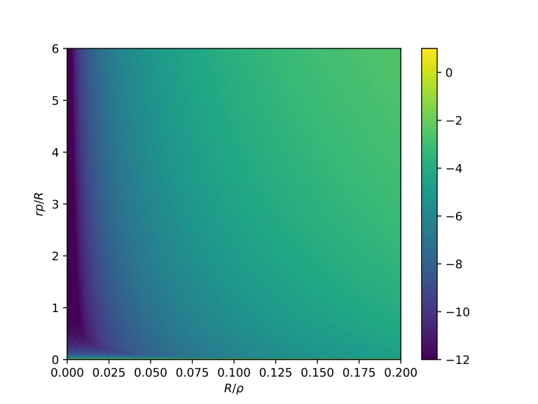
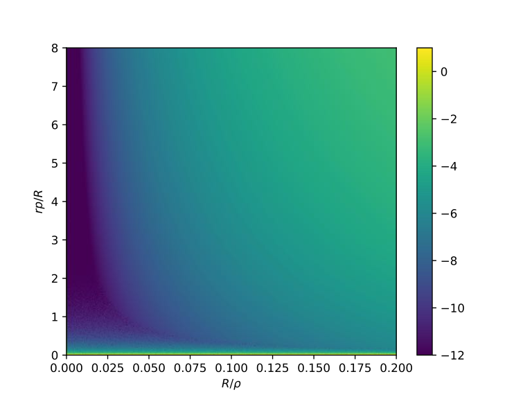
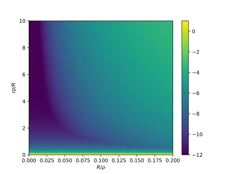
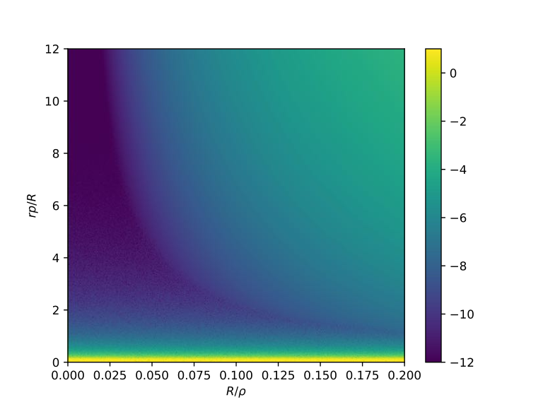
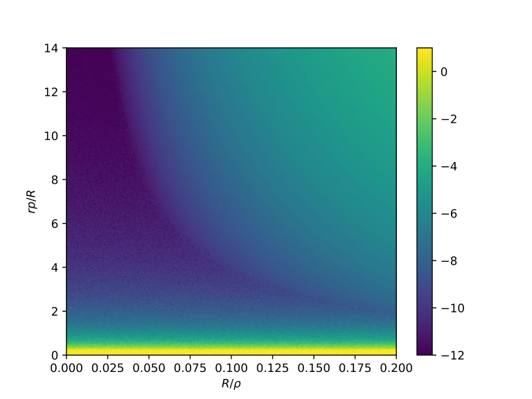
There are several important observations to make from these plots:
- •
Extrapolation error decreases as decreases, as expected.
- •
For a fixed value of , the extrapolation error decreases rapidly as decreases, up to a certain value . This is somewhat counterintuitive, since this means placing points closer together and extrapolating a further distance relative to . For a fixed in exact arithmetic, letting the interpolation interval size tend to zero produces an order Taylor expansion of the solution centered at the interval’s origin, which accounts for this phenomenon.
- •
Beyond , the extrapolation error increases. The effects of finite precision eventually pollutes the convergence behavior described above. Moreover, the spacing appears to be a function of . For , can be reduced to without any numerical issues, but by , only is a safe choice for extrapolation.
We do not aim to rigorously analyze these phenomena in this work. We highlight them to provide empirical evidence that equispaced extrapolation is a reasonable, but not optimal, choice for our problem of singular/near-singular integration and to provide some intuition for our parameter choices.
The following simple result describes the behavior of the extrapolation error in Eq. 17.
Theorem 4.2.
Let be the solution to Eq. 2 given by Eq. 4, restricted to the line in 3D intersecting , let be given by
| (22) |
where is the closest point on to , , , is the outward surface normal at , and let be bounded above by on the interval . Let be the -th order polynomial interpolant of constructed from the check points , where . Then the extrapolation error associated with hedgehog behaves according to:
| (23) |
where .
Proof.
We know that for a smooth function and points in a 1D interval , for some , the following relation holds for all :
| (24) |
Let be the th order polynomial interpolating the points . In the hedgehog setup, since is the distance of the furthest check point to , we know that for each . Since is harmonic, and therefore , in , can be uniformly bounded on by some constant , Noting that and yields our result. ∎
For fixed values of and , as we let , the extrapolation error is bounded by . In practice, however, this means that we can choose and to minimize the constant factor in Theorem 4.2. Since , must be chosen to balance out the contribution of , yet our extrapolation study shows that we can’t simply set . We therefore choose for and 8, motivated by Figs. 7(a) and 7(b). Moreover, since , we can choose , which allows and to decay at the same rate. The advantage of choosing is that is a single parameter that controls the accuracy of hedgehog . Since we have fixed the quadrature order to satisfy the assumption in Section 3.2.2, a smaller value of will trigger more upsampling in Algorithm 3, keeping quadrature error fixed while reducing extrapolation error.
It is important to keep in mind that Theorem 4.2 only provides insight for moderate values of ; our conclusions are largely irrelevant for large . We use and , leaving the construction of an optimal extrapolation extrapolation scheme to future work.
4.3 Limitations
Our error discussion reveals several limitations of our method. The first and most apparent shortcoming is that extrapolation instability fundamentally limits convergence order. However, for reasonable orders of convergence, up to 14, we have discussed an empirical scheme to choose parameters to maximize the available convergence behavior. Moreover, low-order surface geometries used in engineering applications will likely limit the convergence rate before it is limited by the extrapolation order, making this a non-issue in practical scenarios.
Another downside of the chosen extrapolation approach is lack of direct extension of hedgehog to oscillatory problems like the Helmholtz equation. Due to the limitation on the values of , we can’t guarantee the ability to resolve high-frequency oscillations in the solution. A new extrapolation procedure is required to do so robustly without compromising efficiency.
In [68], the authors demonstrate a relationship between the truncation error of a QBX expansion and the local curvature of . Our scheme also is susceptible to this form of error and we do not address nor analyze this in this work. This is a subtle problem that requires a detailed analysis of the surface geometry with respect to the chosen extrapolation scheme. Another limitation is the lack of an accurate error estimate to serve as an upsampling criteria in place of the criteria in Section 3.2.2, such as [35]. Extending [35] to 3D surfaces is non-trivial and whether the size of would be reduced enough to outweigh the added cost of the additional Newton iterations required by their scheme remains to be seen.
Finally, for certain accuracy targets and geometries, the algorithm above may lead to an impractically high number of patches in and . Geometries with nearly-touching non-local regions, as shown in Fig. 12, will see large amounts of refinement. If the nearly-touching embeddings are close enough, i.e., less than apart, there is little hope of an accurate solution with a fixed computational budget. We allow the user to enforce a minimal patch size , limiting the time and memory consumption at the expense of not reaching the requested target accuracy.
5 Complexity
In this section, we summarize the complexity of the algorithms required by hedgehog . We present a detailed complexity analysis in [46, Section 3]. The input to our overall algorithm is a domain boundary with patches and boundary condition . The parameters that directly impact complexity are:
- •
The number of patches after admissibility refinement. This is a function of , the geometry of , the definition of , and the choices of parameters and in check point construction.
- •
Quadrature order and the degree of smoothness of and . We assume that is sufficiently high to obtain optimal error behavior for a given by letting in Eq. 21.
- •
hedgehog interpolation order .
- •
The numbers of evaluation points in different zones , , and , with .
The complexity is also affected by the geometric characteristics of as described in [46, Section 3].
- •
Admissibility. The complexity of this step is , with constants dependent on , and . The logarithmic factor is due to use of an AABB tree for closest surface point queries.
- •
Upsampling. The complexity of upsampling is , where is the largest upsampling ratio. The logarithmic factor appears for similar reason to admissibility, with constants that depend on geometric parameters and the boundary condition through the error estimate of Section 4. We show that the upsampling ratio is independent of in [46, Section 3].
- •
Point marking. Identifying which zone an evaluation point belongs to ( or ) depends on and the total number of points to be classified . The complexity is with constants dependent on geometric parameters, due to the cost of closest surface point queries.
- •
Far, intermediate and near zone integral evaluation. The complexity of these components depends on and , and respectively, with the general form , where is the number of evaluation points in the corresponding class. For the far field, . For the intermediate evaluation, and ; finally, for the near zone, and . If is chosen appropriately, the intermediate and near zone error is .
- •
GMRES solve. Due to the favorable conditioning of the double-layer formulation in Eq. 5, GMRES converges rapidly to a solution in a constant number of iterations for a given that is independent of . This means that the complexity to solve Eq. 5 is asymptotically equal (up to a constant dependent on ) to the complexity equal to a near-zone evaluation with .
- •
Evaluation on uniform point distribution In many applications, one would like the value of the solution due to a density at a collection of points uniformly distributed throughout the domain . When the number of such targets is chosen to match the resolution of the surface discretization, the overall complexity of solution evaluation is .
6 Results
We now demonstrate the accuracy and performance of hedgehog to evaluate singular/near-singular layer potentials on various complex geometries to solve the integral equation in Eq. 5 and evaluate the solution as defined in Eq. 4.
6.1 Classical convergence with patch refinement
We will first demonstrate the numerical convergence behavior of hedgehog . As discussed in [36, Section 3.1], approximation-based schemes such as hedgehog do not converge classically but do so up to a controlled precision if and scale with proportional to the patch size. In order to observe classical convergence as we refine , we must allow and to decrease slower than , such as with rate . In this section, we choose the hedgehog parameters and proportional to to achieve this and demonstrate numerical convergence with refinement of .
In our examples, we use analytic solutions to Eq. 2 obtained as sums of point charge functions of the form
| (25) |
where the charge locations with strengths are outside of . To construct specific solutions, we sample a sphere of radius one with point charges, as shown in Figures 8 and 9. We choose charge strengths randomly from , where for Laplace problems and for Stokes and elasticity problems.
We use the multipole order with points per leaf box for the kernel-independent FMM . This ensures that the FMM error does not dominate; sufficiently large number of points per leaf box is needed to minimize the additional error due to tree depth. We choose a high quadrature order , or 400 quadrature points per patch in , relative to overall convergence order to satisfy the assumption in Section 3.2.2. We also use two levels of uniform upsampling to demonstrate convergence.
6.1.1. Green’s Identity


| Geometry | PDE | Relative error (Number of patches) | EOC | |||
|---|---|---|---|---|---|---|
| Spheroid | Laplace | (96) | (384) | (1536) | (6144) | 4.77 |
| (Fig. 8-left) | Elasticity | (96) | (384) | (1536) | (6144) | 5.74 |
| Stokes | (96) | (384) | (1536) | (6144) | 5.72 | |
| Torus | Laplace | (32) | (128) | (512) | (2048) | 5.45 |
| (Fig. 8-right) | Elasticity | (32) | (128) | (512) | (2048) | 5.09 |
| Stokes | (32) | (128) | (512) | (2048) | 5.09 | |
We report the accuracy of the hedgehog evaluation scheme in Table 1, where we verify Green’s Identity for a random known function in Eq. 25. We evaluate the Dirichlet and Neumann boundary data due to at the discretization points of and use one-sided hedgehog to evaluate the corresponding single- and double-layer potentials at the same discretization points. With each column of Table 1, we subdivide to more accurately resolve the boundary condition. The error shown in Table 1 is the -relative error in the solution value
| (26) |
where and are the single- and double-layer singular integral operators discretized and evaluated with hedgehog . In these tests, we choose , () and (). We observe roughly th order convergence on both the spheroid and torus test geometries in Fig. 8 for each of the tested PDE’s. In Table 2, we present the number of target points evaluated per second per core with one-sided hedgehog . We see that performance is best for Laplace and worst for elasticity problems, as expected.
| Geometry | PDE | Target points/second/core | |||
|---|---|---|---|---|---|
| Spheroid | Laplace | ||||
| (Fig. 8-left) | Elasticity | ||||
| Stokes | |||||
| Torus | Laplace | ||||
| (Fig. 8-right) | Elasticity | ||||
| Stokes | |||||
6.1.2. Solution via GMRES


| Geometry | PDE | Relative error (Number of patches) | EOC | |||
|---|---|---|---|---|---|---|
| Spheroid (Fig. 8-left) | Laplace | (96) | (384) | (1536) | (6144) | 5.35 |
| Pipe | Laplace | (30) | (120) | (480) | (1920) | 5.92 |
| (Fig. 9-left) | Elasticity | (30) | (120) | (480) | (1920) | 5.45 |
| Stokes | (30) | (120) | (480) | (1920) | 5.43 | |
| Genus 2 | Laplace | (50) | (200) | (800) | (3200) | 8.76 |
| (Fig. 9-right) | Elasticity | (50) | (200) | (800) | (3200) | 6.89 |
| Stokes | (50) | (200) | (800) | (3200) | 6.88 | |
| Geometry | PDE | Target points/second/core | |||
|---|---|---|---|---|---|
| Spheroid | Laplace | ||||
| Pipe | Laplace | ||||
| (Fig. 8-left) | Elasticity | ||||
| Stokes | |||||
| Genus 2 | Laplace | ||||
| (Fig. 8-right) | Elasticity | ||||
| Stokes | |||||
We report the accuracy of the hedgehog scheme when used to solve Eq. 2 via the integral equation in Eq. 5. Two-sided hedgehog is used in the matrix-vector multiply inside GMRES to solve Eq. 5 for the values of the density at the discretization points. Then one-sided hedgehog is used to evaluate Eq. 8 at a slightly coarser discretization. Since GMRES minimizes the residual at the original discretization of Eq. 5, this final step prevents an artificially accurate solution by changing discretizations. Table 3 lists the relative error values for the total solve and evaluation steps using Section 3.1 as we refine by subdivision as in the previous section. In these tests, we choose , (), and (). As for previous examples, we observe at least th order convergence on all tested geometries in Fig. 9 and Fig. 8-left and all PDE’s. We include the spheroid example as an additional demonstration of a high accuracy solution via GMRES with our approach. We report the number of target points evaluated per second per core with two-sided hedgehog in Table 4. The results are similar to Table 2; the slower performance is because evaluation via two-sided hedgehog is more expensive than one-sided hedgehog .
6.2 Comparison with [75]
In this section, we compare our method to [75], a previously proposed high-order, kernel-independent singular quadrature method in 3D for complex geometries. These characteristics are similar to hedgehog shares these characteristics. [46, Section 4] presents additional comparisons.
The metric we are interested is cost for a given relative error. Assuming the surface discretization is , we measure the cost of a method as its total wall time during execution divided by the total wall time of an FMM evaluation on the same discretization, . By normalizing by the FMM evaluation cost, we minimize the dependence of the cost on machine- and implementation-dependent machine-dependent parameters.
We run the tests in this section on the spheroid geometry shown in Fig. 8-left. We focus on the singular quadrature scheme of [75]. The near-singular quadrature of [75] is algorithmically similar to hedgehog , but since an expensive singular quadrature rule is used as a part of near-singular evaluation, it has a higher total cost. As a result, the accuracy and cost of near-singular evaluation of [75] is bounded by the accuracy and cost of the singular integration scheme.
To compare the full hedgehog method with [75], we fit polynomial patches to the surface of [76], denoted , to produce during the first step of Section 3.4. We apply the remaining geometry preprocessing algorithms of Section 3.4 to to produce . After producing with two levels of uniform upsampling, we solve Eq. 5 with two-sided hedgehog on and evaluate the solution on the boundary with one-sided hedgehog . We then solve for the solution to Eq. 5 on using [75].
For each of the tests in this section, we choose some initial spacing parameter to discretize the surface of [76], as in [75], and use the upsampled grid and floating partition of unity radius proportional to , as in the original work. We apply hedgehog to and the scheme of [75] to with spacing , for .
As in the previous section, we choose the parameters and of hedgehog to be . For both quadrature methods, we use a multipole order of for PVFMM with at most 250 points in each leaf box.
The results are shown in Fig. 10. From left to right, each plot details the total cost of each scheme, the cost of each subroutine for hedgehog (denoted HH) and the singular quadrature scheme of [75] (denoted POU), and the relative error as a function of and , respectively, for all refinement levels. We plot the cost of both schemes the cost of each algorithmic step as a function of their computed relative error. In each figure, we present results for a Laplace problem (top) and an elasticity problem (bottom).
In Fig. 10, as expected, we observe a higher convergence rate for hedgehog compared to [75]. [75] outperforms hedgehog in terms of cost for all tested discretizations. We observe that the FMM evaluation in Fig. 10 accounts for at least 95% of the hedgehog cost. This means that a local singular quadrature method (based on corrections to an FMM evaluation, Section 1.2) of worse complexity can beat a global method, simply by virtue of reducing the FMM size. By noting the large difference between the hedgehog FMM cost and the hedgehog density interpolation, we can reasonably infer that a local hedgehog scheme should narrow this performance gap and outperform [75] for larger problems, assuming that switching to a local scheme does not dramatically affect error convergence.
6.3 Requested target precision vs. computed accuracy
In this section, we study the performance of the full algorithm outlined in Section 3. We test hedgehog on the torus domain shown in Fig. 8-right. We choose a reference solution of the form of Eq. 25 with a single point charge located at the origin, in the middle of the hole of the torus. We solve the integral equation with two-sided hedgehog and evaluate the singular integral on a distinct discretization with one-sided hedgehog . We choose , and . We select various values for using the plot in Fig. 7(a) to choose to ensure sufficiently accurate extrapolation. We plot the results of our tests in Fig. 11.
We see in Fig. 11-left that we are consistently close to the requested target precision. We see a decline in target points per second per core as accuracy increases in Fig. 11-middle. This is explained by Fig. 11-right, which shows an increase in the size as remains a fixed size. The initial 128 patches in are enough to resolve the boundary condition and , but we need greater quadrature accuracy for lower values of . Decreasing the number of points in passed to the FMM , i.e., decreasing the size of , is the main way to improve performance of our method. This is further indication that a local version of hedgehog will outperform a global approach.
6.4 Full algorithm on interlocking torii
We now demonstrate the full algorithm pipeline on an exterior Laplace problem, whose boundary is defined by four interlocking torii shown in Fig. 12. The domain boundary is contained in the box . The shortest distance between two adjacent torii is less than 10% of a polynomial patch length defining the boundary. We again use a boundary condition of the form Eq. 25 with a single point charge located at , inside the upper half of the second torus from the right in Fig. 12. This problem is challenging due to the nearly touching geometry of the torii, along with the singularity placed close to the boundary. We run the admissibility and adaptive upsampling algorithms outlined in Section 3, solve Eq. 5 using two-sided hedgehog , and evaluate the solution on the boundary using one-sided hedgehog . The absolute error in the -norm of the singular evaluation is plotted on the boundary surface.


Using , , and , we achieve a maximum pointwise error of . GMRES was able to reduce the residual by a factor of over 109 iterations. There are 288768 quadrature points in the coarse discretization, 18235392 quadrature points in the fine discretization, and 3465216 check points used in the two-sided hedgehog evaluation inside GMRES. We evaluate the solved density at 451200 points on the boundary with one-sided hedgehog to produce the render in Fig. 12. On a machine with two Intel Xeon E-2690v2 3.0GHz CPU’s, each with 10 cores, and 100 GB of RAM, the GMRES solve and interior evaluation required 5.7 hours and can evaluate the singular integral at a rate of 1709 target points per second per core.
6.5 Solution on complex geometry

We have demonstrated in [42] a parallel implementation of Section 3.1, applied to simulating red blood cell flows. The surface geometry of the blood vessel shown in Fig. 13 is complex, with rapidly varying curvatures and geometric distortions due to singular vertices in the surface mesh. Since the surface is admissible, we are able to apply parallel hedgehog directly without geometric preprocessing to solve an interior Dirichlet Stokes problem. We use , , and as simulation parameters.
Using 32 machines each with twenty 2.6 Ghz cores with 100GB of RAM, we achieve a maximum pointwise error of when solving a Stokes problem with constant density. We then place a random vector point charge two patch lengths away (relative to the patches in ) from the domain boundary (on the left side of Fig. 13, solve Eq. 5 using two-sided hedgehog , and evaluate the solution on the boundary using one-sided hedgehog . The absolute error in the -norm of the singular evaluation is plotted on the boundary surface. There are 10,485,760 quadrature points in the coarse discretization, 167,772,160 quadrature points in the fine discretization, and 125,829,120 check points used in the two-sided hedgehog evaluation inside GMRES. We evaluate the solved density at 209,715,200 points on the boundary with one-sided hedgehog to produce the render in Fig. 12. We achieve a maximum pointwise error of and can evaluate the singular integral at rate of 3529 target points per second per core.
7 Conclusion
We have presented hedgehog , a fast, high-order, kernel-independent, singular/near-singular quadrature scheme for elliptic boundary value problems in 3D on complex geometries defined by piecewise tensor-product polynomial surfaces. The primary advantage of our approach is algorithmic simplicity: the algorithm can implemented easily with an existing smooth quadrature rule, a point FMM and 1D and 2D interpolation schemes. We presented fast geometry processing algorithms to guarantee accurate singular/near-singular integration, adaptively upsample the discretization and query local surface patches. We then evaluated hedgehog in various test cases, for Laplace, Stokes, and elasticity problems on various patch-based geometries and compared our approach with [75].
[42] demonstrates a parallel implementation of hedgehog , but the geometric preprocessing and adaptive upsampling algorithms presented in Section 3 are not parallelized. This is a requirement to solve truly large-scale problems that exist in engineering applications. Our method can also be easily restructured as a local method. The comparison in Section 6.2 highlights an important point: a local singular quadrature method can outperform a global method for moderate accuracies, even when the local scheme is asymptotically slower. This simple change can also dramatically improve both the serial performance and the parallel scalability of hedgehog shown in [42], due to the decreased communication of a smaller parallel FMM evaluation. The most important improvement to be made, however, is the equispaced extrapolation. Constructing a superior extrapolation procedure, optimized for the boundary integral context, is the main focus of our current investigations.
8 Acknowledgements
We would like to thank Michael O’Neil, Dhairya Malhotra, Libin Lu, Alex Barnett, Leslie Greengard, Michael Shelley for insightful conversations, feedback and suggestions regarding this work. We would also like to thank the NYU HPC team, and Shenglong Wang in particular, for great support throughout the course of this work, and the helpful feedback of the anonymous reviewers. This work was supported by NSF grant DMS-1821334.
Appendix A Derivation of 4.1
We are interested in computing the error incurred when approximating a 2D surface integral with an interpolatory quadrature rule. In 1D on the interval , we’re interested in the quantity
| (27) | ||||
| where | ||||
| (28) | ||||
| (29) | ||||
for quadrature weights for a -point quadrature rule. For a 2D double integral, we define a similar relationship between the remainder, the exact integral and the th order quadrature rule:
| (31) | ||||
| where | ||||
| (32) | ||||
| (33) | ||||
For a function of two variables , we will denote as integration with respect to the variable only, which produces a function of . The same subscript notation applies to and and use similar notation for : we apply the 1D functional to the variable in the subscript, producing a 1D function in the remaining variable. We observe that
| (34) |
Following the discussion in [3], we substitute into Eq. 34 and have
| (35) | ||||
| (36) | ||||
| (37) |
We assume that the higher-order “remainder of remainder” term contributes negligibly to the error. Although it has been shown that this term has a non-trivial contribution to a tight error estimate [23], we are able to provide a sufficiently tight upper bound. For large , the quadrature rule approaches the value of the integral, i.e., for , we’re left with:
| (38) | ||||
| and hence: | ||||
| (39) | ||||
where means "approximately less than or equal to." From [64, Theorem 5.1], we recall that for a 1D function defined on , if is computed with Clenshaw-Curtis quadrature, is and on for real finite , then for sufficiently large , the following inequality holds
| (40) |
where . We’re interested in integrating a function over an interval for various . If is and on for a real constant independent of , then we can define on and apply Eq. 40:
| (41) |
This follows directly from the proof of [64, Theorem 4.2] applied to by replacing with and noting that . The change of variables produces the first power of , while each of the integration by parts produces an additional power of . In the context of hedgehog , the size of is proportional to the edge length of the subdomain outlined in Section 2.2.
Applying Eq. 41 to Eq. 39, and again letting , gives us
| (42) |
where and for fixed values of . If we can choose a that is strictly greater than and for any in , we are left with
| (43) |
Applying this to the integration of double layer potentials, we can simply let be the largest variation of the th partial derivatives of the integrand of any single patch in Eq. 7. In fact, we know that this value is achieved at the projection of on the patch closest to , i.e., . We can also choose to observe standard high-order convergence as a function of patch domain size, which we summarize in the following theorem. The smoothness and bounded variation assumptions required to apply Eq. 40 to our layer potential follow directly from the smoothness of in . Our heuristic directly follows.
References
- AFAH+ [19] Mustafa Abduljabbar, Mohammed Al Farhan, Noha Al-Harthi, Rui Chen, Rio Yokota, Hakan Bagci, and David Keyes. Extreme scale FMM-accelerated boundary integral equation solver for wave scattering. SIAM Journal on Scientific Computing, 41(3):C245–C268, 2019.
- AH [09] Kendall Atkinson and Weimin Han. Numerical solution of Fredholm integral equations of the second kind. In Theoretical Numerical Analysis, pages 473–549. Springer, 2009.
- aKT [17] Ludvig af Klinteberg and Anna-Karin Tornberg. Error estimation for Quadrature by Expansion in layer potential evaluation. Advances in Computational Mathematics, 43(1):195–234, 2017.
- aKT [18] Ludvig af Klinteberg and Anna-Karin Tornberg. Adaptive Quadrature by Expansion for layer potential evaluation in two dimensions. SIAM Journal on Scientific Computing, 40(3):A1225–A1249, 2018.
- Alp [99] Bradley K Alpert. Hybrid Gauss-trapezoidal quadrature rules. SIAM Journal on Scientific Computing, 20(5):1551–1584, 1999.
- Bar [14] Alex H Barnett. Evaluation of layer potentials close to the boundary for Laplace and Helmholtz problems on analytic planar domains. SIAM Journal on Scientific Computing, 36(2):A427–A451, 2014.
- BB [08] Alex H Barnett and Timo Betcke. Stability and convergence of the method of fundamental solutions for Helmholtz problems on analytic domains. Journal of Computational Physics, 227(14):7003–7026, 2008.
- BBHP [19] Alex Bespalov, Timo Betcke, Alexander Haberl, and Dirk Praetorius. Adaptive BEM with optimal convergence rates for the Helmholtz equation. Computer Methods in Applied Mechanics and Engineering, 346:260–287, 2019.
- Bea [04] J Thomas Beale. A grid-based boundary integral method for elliptic problems in three dimensions. SIAM Journal on Numerical Analysis, 42(2):599–620, 2004.
- BG [12] James Bremer and Zydrunas Gimbutas. A Nyström method for weakly singular integral operators on surfaces. Journal of computational physics, 231(14):4885–4903, 2012.
- BG [13] James Bremer and Zydrunas Gimbutas. On the numerical evaluation of the singular integrals of scattering theory. Journal of Computational Physics, 251:327–343, 2013.
- BHP [19] Timo Betcke, Alexander Haberl, and Dirk Praetorius. Adaptive boundary element methods for the computation of the electrostatic capacity on complex polyhedra. arXiv preprint arXiv:1901.08393, 2019.
- BK [01] Oscar P Bruno and Leonid A Kunyansky. A fast, high-order algorithm for the solution of surface scattering problems: basic implementation, tests, and applications. Journal of Computational Physics, 169(1):80–110, 2001.
- BL [13] Oscar P Bruno and Stéphane K Lintner. A high-order integral solver for scalar problems of diffraction by screens and apertures in three-dimensional space. Journal of Computational Physics, 252:250–274, 2013.
- BYW [16] J Thomas Beale, Wenjun Ying, and Jason R Wilson. A simple method for computing singular or nearly singular integrals on closed surfaces. Communications in Computational Physics, 20(3):733–753, 2016.
- CDC [17] Stéphanie Chaillat, Luca Desiderio, and Patrick Ciarlet. Theory and implementation of H-matrix based iterative and direct solvers for Helmholtz and elastodynamic oscillatory kernels. Journal of Computational physics, 351:165–186, 2017.
- CDLL [17] Stéphanie Chaillat, Marion Darbas, and Frédérique Le Louër. Fast iterative boundary element methods for high-frequency scattering problems in 3D elastodynamics. Journal of Computational Physics, 341:429–446, 2017.
- [18] Camille Carvalho, Shilpa Khatri, and Arnold D Kim. Asymptotic analysis for close evaluation of layer potentials. Journal of Computational Physics, 355:327–341, 2018.
- [19] Camille Carvalho, Shilpa Khatri, and Arnold D Kim. Asymptotic approximations for the close evaluation of double-layer potentials. arXiv preprint arXiv:1810.02483, 2018.
- DT [16] Laurent Demanet and Alex Townsend. Stable extrapolation of analytic functions. arXiv preprint arXiv:1605.09601, 2016.
- EGK [13] Charles L Epstein, Leslie Greengard, and Andreas Klockner. On the convergence of local expansions of layer potentials. SIAM Journal on Numerical Analysis, 51(5):2660–2679, 2013.
- EJJ [08] David Elliott, Barbara M Johnston, and Peter R Johnston. Clenshaw–Curtis and Gauss–Legendre quadrature for certain boundary element integrals. SIAM Journal on Scientific Computing, 31(1):510–530, 2008.
- EJJ [15] David Elliott, Barbara M Johnston, and Peter R Johnston. A complete error analysis for the evaluation of a two-dimensional nearly singular boundary element integral. Journal of Computational and Applied Mathematics, 279:261–276, 2015.
- Far [88] Gerald Farin. Curves and Surfaces for Computer Aided Geometric Design: A Practical Guide. Academic Press Professional, Inc., San Diego, CA, USA, 1988.
- GG [04] Mahadevan Ganesh and Ivan G Graham. A high-order algorithm for obstacle scattering in three dimensions. Journal of Computational Physics, 198(1):211–242, 2004.
- GR [87] Leslie Greengard and Vladimir Rokhlin. A fast algorithm for particle simulations. Journal of computational physics, 73(2):325–348, 1987.
- GT [19] Abinand Gopal and Lloyd N Trefethen. Solving Laplace problems with corner singularities via rational functions. arXiv preprint arXiv:1905.02960, 2019.
- HCB [05] Thomas JR Hughes, John A Cottrell, and Yuri Bazilevs. Isogeometric analysis: CAD, finite elements, NURBS, exact geometry and mesh refinement. Computer methods in applied mechanics and engineering, 194(39-41):4135–4195, 2005.
- HO [08] Johan Helsing and Rikard Ojala. On the evaluation of layer potentials close to their sources. Journal of Computational Physics, 227(5):2899–2921, 2008.
- HRS [19] Jeremy G Hoskins, Vladimir Rokhlin, and Kirill Serkh. On the numerical solution of elliptic partial differential equations on polygonal domains. SIAM Journal on Scientific Computing, 41(4):A2552–A2578, 2019.
- HW [08] George C Hsiao and Wolfgang L Wendland. Boundary integral equations. Springer, 2008.
- JKSH [13] Alec Jacobson, Ladislav Kavan, and Olga Sorkine-Hornung. Robust inside-outside segmentation using generalized winding numbers. ACM Transactions on Graphics (TOG), 32(4):33, 2013.
- JTYO [03] Seppo Järvenpää, Matti Taskinen, and Pasi Ylä-Oijala. Singularity extraction technique for integral equation methods with higher order basis functions on plane triangles and tetrahedra. International journal for numerical methods in engineering, 58(8):1149–1165, 2003.
- JTYO [06] Seppo Jarvenpaa, Matti Taskinen, and Pasi Ylä-Oijala. Singularity subtraction technique for high-order polynomial vector basis functions on planar triangles. IEEE transactions on antennas and propagation, 54(1):42–49, 2006.
- KB [19] Ludvig af Klinteberg and Alex H Barnett. Accurate quadrature of nearly singular line integrals in two and three dimensions by singularity swapping. arXiv preprint arXiv:1910.09899, 2019.
- KBGO [13] Andreas Klöckner, Alexander Barnett, Leslie Greengard, and Michael O’Neil. Quadrature by Expansion: A new method for the evaluation of layer potentials. Journal of Computational Physics, 252:332–349, 2013.
- KKCC [20] Shilpa Khatri, Arnold D Kim, Ricardo Cortez, and Camille Carvalho. Close evaluation of layer potentials in three dimensions. Journal of Computational Physics, 423:109798, 2020.
- KR [97] Sharad Kapur and Vladimir Rokhlin. High-order corrected trapezoidal quadrature rules for singular functions. SIAM Journal on Numerical Analysis, 34(4):1331–1356, 1997.
- Kre [99] Rainer Kress. Linear integral equations, volume 82 of applied mathematical sciences, 1999.
- LB [16] Yuxiang Liu and Alex H Barnett. Efficient numerical solution of acoustic scattering from doubly-periodic arrays of axisymmetric objects. Journal of Computational Physics, 324:226–245, 2016.
- Lév [15] Bruno Lévy. Geogram, 2015.
- LMR+ [19] Libin Lu, Matthew J Morse, Abtin Rahimian, Georg Stadler, and Denis Zorin. Scalable simulation of realistic volume fraction red blood cell flows through vascular networks. arXiv preprint arXiv:1909.11085, 2019.
- MB [15] Dhairya Malhotra and George Biros. PVFMM: A parallel kernel independent FMM for particle and volume potentials. Communications in Computational Physics, 18(3):808–830, 2015.
- MCIGO [19] Dhairya Malhotra, Antoine Cerfon, Lise-Marie Imbert-Gérard, and Michael O’Neil. Taylor states in stellarators: A fast high-order boundary integral solver. arXiv preprint arXiv:1902.01205, 2019.
- Mik [14] Solomon Grigorevich Mikhlin. Integral equations: and their applications to certain problems in mechanics, mathematical physics and technology, volume 4. Elsevier, 2014.
- MRZ [20] Matthew J. Morse, Abtin Rahimian, and Denis Zorin. Supplementary material for: A robust solver for elliptic PDEs in 3D complex geometries. https://cims.nyu.edu/gcl/papers/2020-qbkix3d-supplementary.pdf, 2020.
- Néd [01] Jean-Claude Nédélec. Acoustic and electromagnetic equations, volume 144 of applied mathematical sciences, 2001.
- [48] Constantine Pozrikidis. Boundary integral and singularity methods for linearized viscous flow. Cambridge University Press, 1992.
- [49] Costas Pozrikidis. Boundary Integral and Singularity Methods for Linearized Viscous Flow. Cambridge University Press, 1992.
- PP [82] Vladimir Zalmanovich Parton and Petr Il’ič Perlin. Integral equations in elasticity. Imported Pubn, 1982.
- PTK [11] Rodrigo B Platte, Lloyd N Trefethen, and Arno BJ Kuijlaars. Impossibility of fast stable approximation of analytic functions from equispaced samples. SIAM review, 53(2):308–318, 2011.
- QB [14] Bryan Quaife and George Biros. High-volume fraction simulations of two-dimensional vesicle suspensions. Journal of Computational Physics, 274:245–267, 2014.
- RBZ [18] Abtin Rahimian, Alex Barnett, and Denis Zorin. Ubiquitous evaluation of layer potentials using Quadrature by Kernel-Independent Expansion. BIT Numerical Mathematics, 58(2):423–456, 2018.
- RKO [17] Manas Rachh, Andreas Klöckner, and Michael O’Neil. Fast algorithms for Quadrature by Expansion I: Globally valid expansions. Journal of Computational Physics, 345:706–731, 2017.
- RS [17] Manas Rachh and Kirill Serkh. On the solution of Stokes equation on regions with corners. arXiv preprint arXiv:1711.04072, 2017.
- Sam [06] Hanan Samet. Foundations of multidimensional and metric data structures. Morgan Kaufmann, 2006.
- ŚBA+ [15] Wojciech Śmigaj, Timo Betcke, Simon Arridge, Joel Phillips, and Martin Schweiger. Solving boundary integral problems with BEM++. ACM Transactions on Mathematical Software (TOMS), 41(2):6, 2015.
- Ser [17] Kirill Serkh. On the solution of elliptic partial differential equations on regions with corners II: Detailed analysis. Applied and Computational Harmonic Analysis, 2017.
- Ser [18] Kirill Serkh. On the solution of elliptic partial differential equations on regions with corners III: curved boundaries. Manuscript in preparation, 2018.
- [60] Kirill Serkh and Vladimir Rokhlin. On the solution of elliptic partial differential equations on regions with corners. Journal of Computational Physics, 305:150–171, 2016.
- [61] Kirill Serkh and Vladimir Rokhlin. On the solution of the Helmholtz equation on regions with corners. Proceedings of the National Academy of Sciences, 113(33):9171–9176, 2016.
- ST [18] Michael Siegel and Anna-Karin Tornberg. A local target specific quadrature by expansion method for evaluation of layer potentials in 3D. Journal of Computational Physics, 364:365–392, 2018.
- TB [19] Svetlana Tlupova and J Thomas Beale. Regularized single and double layer integrals in 3D Stokes flow. Journal of Computational Physics, 2019.
- Tre [08] Lloyd N Trefethen. Is Gauss quadrature better than Clenshaw–Curtis? SIAM review, 50(1):67–87, 2008.
- TRH [16] Matthias Taus, Gregory J Rodin, and Thomas JR Hughes. Isogeometric analysis of boundary integral equations: High-order collocation methods for the singular and hyper-singular equations. Mathematical Models and Methods in Applied Sciences, 26(08):1447–1480, 2016.
- TW [91] Lloyd N Trefethen and JAC Weideman. Two results on polynomial interpolation in equally spaced points. Journal of Approximation Theory, 65(3):247–260, 1991.
- WK [18] Matt Wala and Andreas Klöckner. A fast algorithm with error bounds for Quadrature by Expansion. Journal of Computational Physics, 374:135–162, 2018.
- [68] Matt Wala and Andreas Klöckner. A fast algorithm for Quadrature by Expansion in three dimensions. Journal of Computational Physics, 388:655–689, 2019.
- [69] Matt Wala and Andreas Klöckner. Optimization of fast algorithms for global Quadrature by Expansion using target-specific expansions. Journal of Computational Physics, page 108976, 2019.
- WK [20] Matt Wala and Andreas Klöckner. On the approximation of local expansions of laplace potentials by the fast multipole method. arXiv preprint arXiv:2008.00653, 2020.
- WTG [12] Marcus Webb, Lloyd N Trefethen, and Pedro Gonnet. Stability of barycentric interpolation formulas for extrapolation. SIAM Journal on Scientific Computing, 34(6):A3009–A3015, 2012.
- WZBV [20] Bowei Wu, Hai Zhu, Alex Barnett, and Shravan Veerapaneni. Solution of stokes flow in complex nonsmooth 2d geometries via a linear-scaling high-order adaptive integral equation scheme. Journal of Computational Physics, page 109361, 2020.
- XG [10] Hong Xiao and Zydrunas Gimbutas. A numerical algorithm for the construction of efficient quadrature rules in two and higher dimensions. Computers & mathematics with applications, 59(2):663–676, 2010.
- YBZ [04] Lexing Ying, George Biros, and Denis Zorin. A kernel-independent adaptive fast multipole algorithm in two and three dimensions. Journal of Computational Physics, 196(2):591–626, 2004.
- YBZ [06] Lexing Ying, George Biros, and Denis Zorin. A high-order 3D boundary integral equation solver for elliptic PDEs in smooth domains. Journal of Computational Physics, 219(1):247–275, 2006.
- YZ [04] Lexing Ying and Denis Zorin. A simple manifold-based construction of surfaces of arbitrary smoothness. In ACM Transactions on Graphics (TOG), volume 23, pages 271–275. ACM, 2004.
- ZMBF [16] Jürgen Zechner, Benjamin Marussig, Gernot Beer, and Thomas-Peter Fries. The isogeometric Nyström method. Computer methods in applied mechanics and engineering, 308:212–237, 2016.