Archipelagos of Total Bound and Free Entanglement. II

Let us begin by indicating the first model of a bipartite mixed state explicitly analyzed by Li and Qiao in their recent paper “Separable Decompositions of Bipartite Mixed States” Li and Qiao 2018a, and also in our preceding preprint Slater 2020. It took the form of the $2\times 4$ dimensional mixed (qubit-ququart) state,

where $t_{\mu}\neq 0$, $t_{\mu}\in\mathbb{R}$, and $\sigma_{i}$ and $\lambda_{\nu}$ are SU(2) (Pauli matrix) and SU(4) generators, respectively (cf. Singh et al. 2019).

Li and Qiao found that equation (1) represents a physical state when the $8\times 8$ density matrix $\rho_{AB}^{(1)}$ is positive semidefinite, that is if

Figure 1 shows the convex set of possible physical states representable by $\rho_{AB}^{(1)}$. Let us now–to proceed in a probabilistic framework–standardize (dividing by one-half) the three-dimensional Euclidean volume of the possible physical states of $\rho_{AB}^{(1)}$ to equal 1.

Li and Qiao also established that $\rho_{AB}^{(1)}$ has positive (semidefinite) partial transposition, so the well-known PPT criterion could not be used to help determine whether any specific state is entangled or separable. Further, they asserted (Li and Qiao 2018a, eq. (59)) that $\rho_{AB}$ is entangled when

where they (correctly, we claim) associate the quantity $\frac{1}{27}$ with the qubit and (incorrectly) the $\Big(\frac{2}{27}\Big)^{2}$ with the ququart.

Subsequent analyses of ours–using the well-known necessary and sufficient conditions for positive-semidefiniteness that all leading minors be nonnegative Prussing 1986–firmly indicated that these constraints should be replaced by the decidedly weaker ones,

(We speculated that the $\Big(\frac{2}{27}\Big)^{2}$ bound could have, in fact, been obtained if some different/nonstandard orderings–other than the one we employed, given in (Sbaih et al. 2013, eq. (3))–of the fifteen SU(4) generators had been employed. But for none of the possible three-member 455 subsets of the fifteen generators were such bounds found. Interestingly, the discussion as to the variable ranges before eq. (67) in Li and Qiao 2018a precisely agrees–using the relation $t_{i}=\alpha_{i}\beta_{i}$ and the bounds $\beta_{1}^{2}+\beta_{3}^{2}\leq\frac{1}{4}$, $\beta_{2}^{2}\leq\frac{1}{4}$ and $\alpha_{1}^{2}+\alpha_{2}^{2}+\alpha_{3}^{2}\leq 1$–with that we obtain using the leading-minors approach. However, the conclusions of Li and Qiao from these ranges are somewhat surprisingly incorrect–especially given their preceding detailed argument–as the maximization of $(|t_{1}|+|t_{2}|+|t_{3}|)^{2}$ and $(t_{1}t_{2}t_{3})^{2}$ subject to the joint imposition of both constraints yields $\frac{1}{2}$ and $\frac{1}{6912}$–and not 1 and $\frac{4}{19683}$, respectively.)

This replacement of entanglement bounds immediately leads us to a remarkable result. While the constraint $(|t_{1}|+|t_{2}|+|t_{3}|)^{2}>1\hskip 7.22743pt$ given by Li and Qiao proved to be unenforceable/irrelevant (perhaps an indication of its incorrectness), the weaker constraint $(|t_{1}|+|t_{2}|+|t_{3}|)^{2}>\frac{1}{2}$ gives us a bound-entanglement qubit-ququart probability of $\frac{2}{3}\left(\sqrt{2}-1\right)\approx 0.276142$ and an accompanying pair (archipelago) of corresponding islands (Fig. 2).

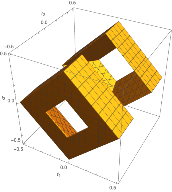
Use of the further (multiplicative) constraint $(t_{1}t_{2}t_{3})^{2}>\frac{1}{6912}$ gives us a more complicated (and smaller) bound-entanglement probability ($\approx 0.12668688797$) of

,

where $p=\sqrt{9-2\sqrt{3}}\approx 2.35285$, and the polylogarithmic (dilogarithmic) function is employed. The corresponding archipelago diagram is Fig. 3.

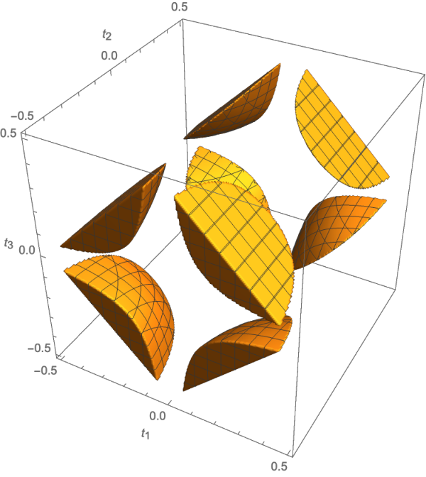
In Figure 4, we show the bound-entangled archipelago of those qubit-ququart states satisfying the constraint $(|t_{1}|+|t_{2}|+|t_{3}|)^{2}>\frac{1}{2}$, but now not $(t_{1}t_{2}t_{3})^{2}>\frac{1}{6912}$.

The associated probability is approximately 0.151609 Imp.

Reversing matters, in Figure 5, we show the bound-entangled archipelago of those qubit-ququart states satisfying the constraint $(t_{1}t_{2}t_{3})^{2}>\frac{1}{6912}$ but not $(|t_{1}|+|t_{2}|+|t_{3}|)^{2}>\frac{1}{2}$. The associated probability is quite negligible, that is approximately 0.000269161439.

The probability that both (additive and mulitiplicative-type) constraints are satisfied is approximately 0.11265766, and the (total bound) probability that at least one of the two constraints is satisfied is approximately 0.276411536. (An accompanying plot for the first probability appears as a somewhat diminished version of Fig. 3 and an accompanying plot for the second probability appears a somewhat expanded version of Fig. 2.)

Let us now shift–as we had in Slater 2020–to the study of the two-ququart states,

where as before the $\lambda$’s are $SU(4)$ generators. The set of all two-ququart states is delimited by the constraint

That is, the set of possible $\{t_{1},t_{2},t_{3}\}$ comprises the cube $[-\frac{1}{4},\frac{1}{4}]^{3}$. All these states have positive partial transposes, so all entangled states are bound. Then, we have-again using the well-known necessary and sufficient conditions for positive-semidefiniteness that all leading minors be nonnegative Prussing 1986-the corresponding entanglement constraints (cf. eq. (3)),

rather than $\frac{1}{2}$ and $\frac{1}{6912}$ as in the qubit-ququart model. (Again, we note for our maximization procedures, the basic relation in the Li-Qiao framework, $t_{i}=\alpha_{i}\beta_{i}$, together with the bounds, $\alpha_{1}^{2}+\alpha_{3}^{2}\leq\frac{1}{4}$, $\alpha_{2}^{2}\leq\frac{1}{4}$ and $\beta_{1}^{2}+\beta_{3}^{2}\leq\frac{1}{4}$, $\beta_{2}^{2}\leq\frac{1}{4}$ .) The single constraint $(|t_{1}|+|t_{2}|+|t_{3}|)^{2}>\frac{1}{4}$ gives us a bound-entanglement probability of $\frac{1}{6}\approx 0.166666$ and a set of corresponding islands (Fig. 6).

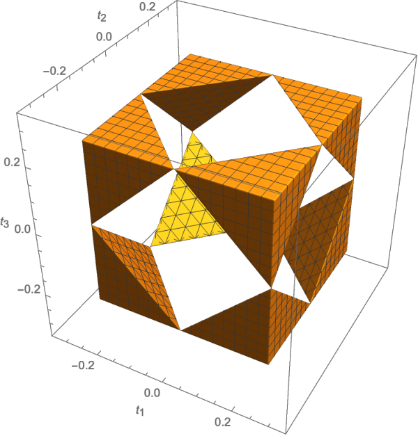
The single constraint $(t_{1}t_{2}t_{3})^{2}>\frac{1}{65536}$ yields a roughly equal-sized bound-entanglement probability of $\frac{1}{4}\left(3-2\log^{2}(2)-\log(4)\right)\approx 0.1632$, and a set of corresponding islands (Fig. 7).

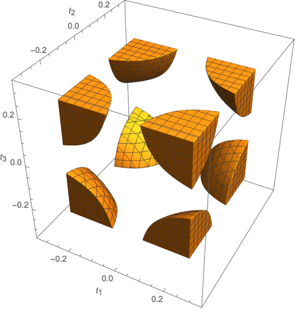
The probability that both (additive and mulitiplicative) constraints are satisfied is approximately 0.149164132389, while the (total bound) probability that either of the two constraints is satisfied is approximately 0.180702437039. These two probabilities, of course, add to $\frac{1}{6}+\frac{1}{4}\left(3-2\log^{2}(2)-\log(4)\right)=\frac{1}{12}\left(11-6\log^{2}(2)-3\log(4)\right)\approx 0.3298665694275933$ (as a matter of Boolean logic, since $(A\land B)\lor(A\lor B)=A\lor B$). Our best current efforts at exactly computing this pair of probabilities yielded expressions employing elliptic integrals plus one-dimensional integrals of $t_{1}$ over $[-\frac{1}{4},\frac{1}{8}(\sqrt{5}-3)]$ and over $[\frac{1}{8}(3-\sqrt{5}),\frac{1}{4}]$, many of the integrands involving the term $\sqrt{64\left(t_{1}-1\right)t_{1}-\frac{1}{t_{1}}+16}$.

In Figure 8, we show the bound-entangled archipelago of those two-ququart states (6) satisfying the constraint $(|t_{1}|+|t_{2}|+|t_{3}|)^{2}>\frac{1}{4}$, but not $(t_{1}t_{2}t_{3})^{2}>\frac{1}{65536}$. The associated probability is approximately 0.0175025342.

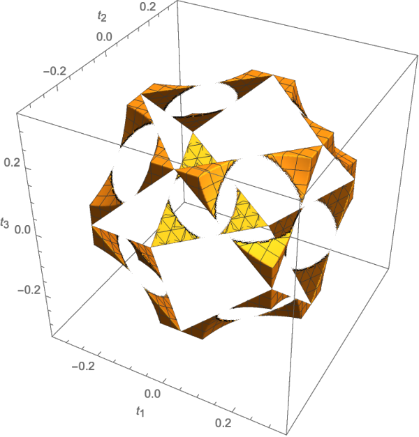
Reversing matters, in Figure 9, we show the bound-entangled archipelago of those two-ququart states satisfying the constraint $(t_{1}t_{2}t_{3})^{2}>\frac{1}{65536}$, but not $(|t_{1}|+|t_{2}|+|t_{3}|)^{2}>\frac{1}{4}$. The associated probability is quite negligible, that is approximately 0.01403577037231.

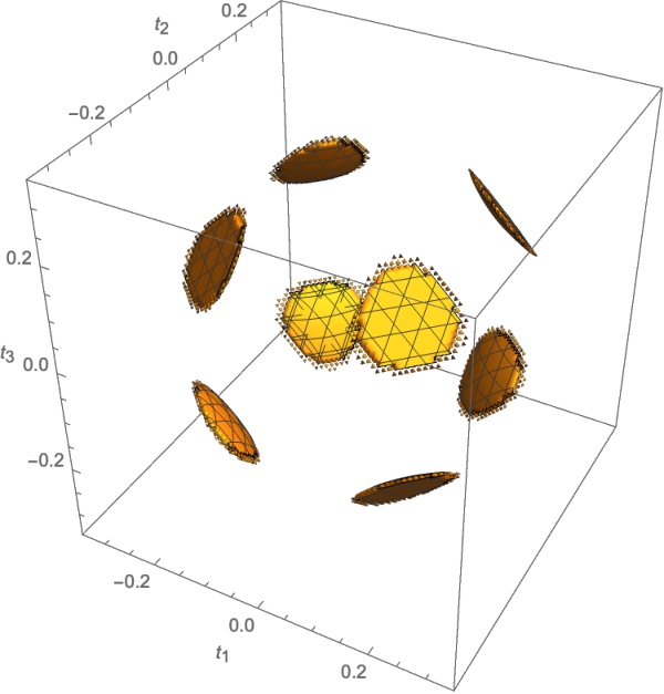
Let us now–somewhat briefly–study a second two-ququart model

The entanglement constraints are

The PPT-probability is $\frac{8}{3\pi}\approx 0.848826$. The total (bound and free) entanglement probability is $\frac{3\pi-4}{3\pi}\approx 0.575587$, while the bound entanglement probability is $\frac{4}{3\pi}\approx 0.424413$. The entangled but not bound states are shown in Fig. 10.

For the convenience of the reader, and since the qubit-ququart and two-ququart analyses in Slater 2020 have now been called into question, let us again present the interesting analyses there, not similarly suspect.

There, we “downgraded” the Li-Qiao qubit-ququart model to simply a two-qubit one,

while employing the entanglement constraints (again consistent with the leading-minors analysis),

Then, we obtained a number of interesting results. Firstly, now only one-half of the physically possible states had positive partial transposes.

Also, imposition of the single (additive) constraint $(|t_{1}|+|t_{2}|+|t_{3}|)^{2}>1$ revealed that the other (non-PPT) half of the states are all entangled, as expected. On the other hand, enforcement of the single (multiplicative) constraint revealed that only 0.3911855600402 of these non-PPT states were entangled. The entangled states again formed an archipelago (Fig. 11), also apparently “jagged” in nature, but now clearly not of a bound-entangled nature (given the two-qubit context). Those two-qubit states which satisfy the $(|t_{1}|+|t_{2}|+|t_{3}|)^{2}>1$ entanglement constraint, but not the $(t_{1}t_{2}t_{3})^{2}>\Big(\frac{1}{27}\Big)^{2}$, one are displayed in Fig. 12. The associated probability is $\frac{1}{2}-0.3911856=0.108814$.

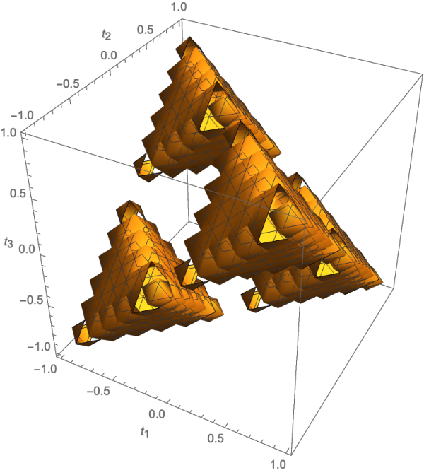
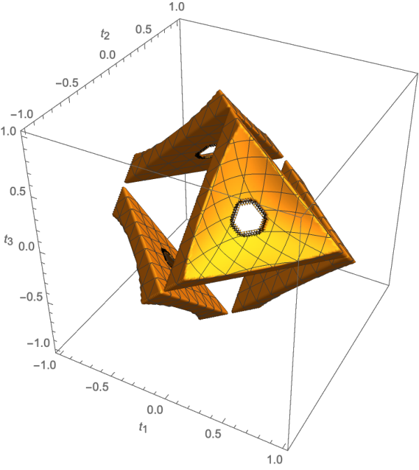
Continuing with our analyses, we have been able to determine that the appropriate (multiplicative) entanglement constraint to employ for the first member,

of the pair of two-qutrit (octahedral and tetrahedral) models of Li and Qiao (Li and Qiao 2018a, sec. 2.3.2) is

and for the second member,

of the pair,

(We achieved these results by maximizing the product $t_{1}t_{2}t_{3}$, subject to the conditions that the parameterized target density matrix and its separable components not lose their positive definiteness properties.)

For the first two-qutrit model (13), we remarkably found the exact same entanglement behavior/probabilities ($\frac{1}{2}$ and 0.3911855600402 and Fig. 12) as we did in the two-qubit analyses. Also, we did not find that the second two-qutrit model (15) evinced any entanglement at all–in accordance with the explicit assertion of Li and Qiao that the state “is separable for all values of $t_{i}$,…”

As an additional two-qutrit exercise, let us consider the model

The associated PPT probability is $\frac{1}{2}+\frac{2}{\pi^{2}}\approx 0.702642$. The pair of entanglement constraints now takes the form

The probability that a state (17) satisfies the multiplicative constraint is 0.490454, while the probability that it satisfies the additive constraint is $1-\frac{8}{3\pi^{2}}\approx 0.72981$. The corresponding bound-entanglement probabilities are 0.205794 and $\frac{1}{2}-\frac{2}{3\pi^{2}}\approx 0.432453$. The entirety of entanglement probability is 0.748599, while the entirety of bound-entangled probability is 0.43549.

In Fig. 13, we show those (free or bound) entangled states satisfying both entanglement constraints.

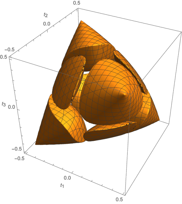
On the other hand, in Fig. 14, we show only bound entangled states satisfying both entanglement constraints.

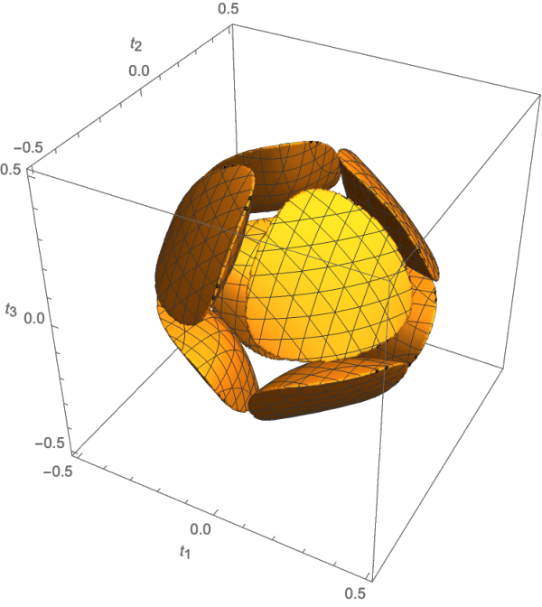
To further pursue these general lines of investigation following the approach of Li and Qiao, we searched for qutrit-ququart models with non-positive-partial-transpose states. One that emerged took the form

with the $\lambda$’s being as before the SU(3) generators and the $\kappa$’s now being the SU(4) generators. The associated PPT-probability is $\frac{1}{2}+\frac{2}{\pi^{2}}\approx 0.848826$. The relevant entanglement constraints are now

The entire (bound and free) entanglement probability based on the union of these two constraints is $\frac{3\pi-4}{3\pi}\approx 0.575587$, while the bound component is $\frac{4}{3\pi}\approx 0.424413$. In fact, the first constraint fully dominates the second one. That is, there are no states entangled in terms of the second constraint that are not entangled in terms of the first. If we employ just the second constraint, then the corresponding entanglement probabilities are 0.304652 and 0.1706.

For the further (now PPT) qutrit-ququart model,

we have found entanglement constraints of the form

where $123018750=2\cdot 3^{9}\cdot 5^{5}$. The associated bound-entanglement probabilities yielded by enforcement of the two constraints individually are 0.639747 and 0.185841, respectively. The first constraint fully dominates the second.

Following and building upon the work of Li and Qiao, all the analyses reported above have involved the three parameters $t_{1},t_{2},t_{3}$, thus, lending results to immediate visualization. In higher-dimensional studies, one would have to resort to cross-sectional examinations, such as Figs. 22 and 23 in Slater 2019, based on the (four parameter) two-ququart Hiesmayr-Löffler “magic simplex” model Hiesmayr and Löffler 2014.

Of course, visualizations are possible in lower (two) dimensions, as well. In fact, we examined the two-qutrit (PPT) model

In doing so, in adopting the primary three-parameter Li-Qiao framework to a two-parameter one, we followed their prescriptions regarding the choice of orthogonal matrices $Q$, following eq. (23) in Li and Qiao 2018b. Such matrices are of dimension $(l+1)\times(l+1)$, where $l$ is the number of parameters. The last row of $Q$ contains non-negative entries. In particular, for the three subsequent (two-qutrit, two-ququart and qutrit-ququart) two-parameter analyses, we employed

The entanglement constraints for the two-parameter model (23) are of the form

The set of possible states of area $\frac{16\pi}{81}\approx 0.620562$ is the circle $16-81t_{1}^{2}-81t_{2}^{2}\geq 0$ of radius $\frac{4}{9}$. The set of unentangled states is the inscribed square with vertices at $(\pm\frac{4}{9},0)$ and $(0,\pm\frac{4}{9})$. This is shown in Fig. 15.

The bound-entangled states, lying outside the inscribed square, are of probability $\frac{\pi-2}{\pi}\approx 0.36338$. The constraint $(|t_{1}|+|t_{2}|)^{2}>\frac{16}{81}$ fully dominates the constraint $(t_{1}t_{2})^{2}>\frac{16}{6561}$ (which itself yields $\frac{2}{3}-\frac{\cosh^{-1}(2)}{\pi}\approx 0.247466$). Those bound-entangled states that are yielded by the dominant constraint $(|t_{1}|+|t_{2}|)^{2}>\frac{16}{81}$, but not by the subdominant constraint $(t_{1}t_{2})^{2}>\frac{16}{6561}$ are displayed in Fig. 16. They are of probability $\frac{-6+\pi+3\cosh^{-1}(2)}{3\pi}\approx 0.115914$.

Let us move on, still within the modified two-parameter Li-Qiao framework to the (PPT) two-ququart model

where the $\kappa$’s as in (19) and (21) represent the $SU(4)$ generators with their standard ordering. The entanglement constraints are of the form

We will find that although the first constraint does not fully dominate the second, it nearly does–except for an archipelago of four regions accounting for only $\frac{7-24\log\left(\frac{4}{3}\right)}{8\left(4-3\log\left(\frac{4}{3}\right)\right)}\approx 0.381063\%$ of the total bound-entangled probability of $\frac{1}{9}\left(4-3\log\left(\frac{4}{3}\right)\right)\approx 0.34855$.

In Fig. 17 we show the square with vertices at $(\pm\frac{1}{4},\pm\frac{1}{4})$, comprising the set of possible states. The four corner triangles of it comprise the bound-entangled states of the noted probability $\frac{1}{9}\left(4-3\log\left(\frac{4}{3}\right)\right)\approx 0.34855$. The eight-sided region consists of the complementary separable states. The constraint $(|t_{1}|+|t_{2}|)^{2}>\frac{49}{576}$ accounts for $\frac{25}{72}\approx 0.347222$, and the constraint $(t_{1}t_{2})^{2}>\frac{1}{2304}$ for $\frac{1}{3}(2-\log(3))\approx 0.300463$. The bound-entangled probability attributable to the $(t_{1}t_{2})^{2}>\frac{1}{2304}$ constraint, but not the other is only $\frac{1}{72}\left(7-24\log\left(\frac{4}{3}\right)\right)\approx 0.0013282$. On the other hand, the bound-entangled probability attributable to the $(|t_{1}|+|t_{2}|)^{2}>\frac{49}{576}$ constraint, but not the other is $\frac{2}{9}\left(\log\left(\frac{27}{8}\right)-1\right)\approx 0.0480878$.

(We also considered several further two-parameter scenarios–these of a hybrid qutrit-ququart character. They largely yielded diagrams of a rather similar nature to Fig. 17.)

It now seems possible to rather readily extend the Li-Qiao framework to further high-dimensional bipartite systems–e. g. qutrit-ququart, qubit-ququint,…other than the specific ones studied above. Of immediate interest for all such systems is the question of to what extent they have positive partial transposes. Then, issues of bound and free entanglement can be addressed.

Let us also raise the question of whether or not the Hiesmayr-Löffler “magic simplices” Hiesmayr and Löffler 2014 and/or the generalized Horodecki states Horodecki et al. 1998 can be studied–through reparameterizations–within the Li-Qiao framework, with consequent answers as to the associated total bound entanglement probabilities. Possibly, then, the new archipelagos might not evince the strong jaggedness previously observed Slater 2019, along the lines of those observed above here. Jaggedness, then, being a feature of incompleteness/non-totality.

The two-qutrit Hiesmayr-Löffler ‘magic simplex model is, expressible, we have found as

(Interestingly, in the three-dimensional matrix [Gell-mann] representation of $SU(3)$, the Cartan subalgebra is the set of linear combinations (with real coefficients) of the two matrices $\lambda_{3}$ and $\lambda_{8}$, which commute with each other.) Here, $t_{1}=t_{4}=t_{6}=\frac{2}{3}\left(Q_{1}-Q_{3}\right),t_{2}=t_{5}=-\frac{2}{3}\left(Q_{1}-Q_{3}\right),t_{3}=t_{8}=-(1/3)+Q_{1}+2Q_{3}$. Further, $t_{9}=\frac{Q_{1}+6Q_{2}+2Q_{3}-1}{\sqrt{3}}$ and $t_{10}=-\frac{Q_{1}+6Q_{2}+2Q_{3}-1}{\sqrt{3}}$.

Six of the eight singular values of the correlation matrix of (28) are $u=\frac{2}{3}\sqrt{\left(Q_{1}-Q_{3}\right){}^{2}}$ and the remaining two are $v=\frac{2}{3}\sqrt{-9Q_{2}-6Q_{3}+3\left(Q_{1}^{2}+\left(3Q_{2}+4Q_{3}-1\right)Q_{1}+9Q_{2}^{2}+4Q_{3}^{2}+6Q_{2}Q_{3}\right)+1}$.

Numerical analyses appear to strongly indicate that one of the corresponding Li-Qiao entanglement constraints is $(2\left|u\right|+6\left|v\right|)^{2}>\frac{1}{144}$.

Gabuldin and Mandilara concluded that the particular bound-entangled states they found in certain analyses of theirs had “negligible volume and that these form tiny ‘islands’ sporadically distributed over the surface of the polytope of separable states” Gabdulin and Mandilara 2019. In a continuous variable study DiGuglielmo et al. 2011, “the tiny regions in parameter space where bound entanglement does exist” were noted.

Let us note the recent posting of a paper entitled ”Entanglement islands in higher dimensions” Almheiri et al. 2019, concerned with the famous information paradox. The authors conclude: “Islands appear in entanglement wedge of the Hawking radiation at late times and this stops the indefinite growth of von Neumann entropy, giving an answer consistent with unitarity and a finite density of states.”

We further observed that the matrix $Q\in SO(4)$,

employed by Li and Qiao (Li and Qiao 2018a, eq. (62)) is a $4\times 4$ Hadamard matrix Horadam 2012. So, we investigated the possibility that by employing the $8\times 8$ Hadamard matrix

we might extend the Li-Qiao framework from a $3=4-1$-dimensional one to an $7=8-1$-dimensional one. Accordingly–as one of eight possible options–we set up the two-qutrit model

where the $\lambda$’s are the $SU(3)$ generators. ($\lambda_{8}$ is the single one not employed.) For this model, we obtained a PPT-probability of 0.662799194015. Our attempts to obtain the corresponding entanglement constraints and entanglement probabilities have so far not yielded numerical results in which we have sufficient confidence to report.