跳到论文正文
W Papers独立论文阅读器 arXiv:2002.04064 论文正文 计算阅读时间 · 0%
引用这篇论文根据当前论文元数据生成,正式投稿前建议核对。


License: arXiv.org perpetual non-exclusive license
arXiv:2002.04064v1 [math.AP] 10 Feb 2020

Regularity of all minimizers of a class of
spectral partition problems

Hugo Tavares Address: Hugo Tavares
CAMGSD and Departamento de Matemática, Instituto Superior Técnico
Pavilhão de Matemática, Av. Rovisco Pais
1049-001 Lisboa, Portugal
Email address: hugo.n.tavares@tecnico.ulisboa.pt
and Alessandro Zilio Address: Alessandro Zilio
(1) Université de Paris, Laboratoire Jacques-Louis Lions (LJLL), F-75013 Paris, France.
(2) Sorbonne Université, CNRS, LJLL, F-75005 Paris, France
Email address: azilio@math.univ-paris-diderot.fr
Date: August 11, 2026
Abstract.

We study a rather broad class of optimal partition problems with respect to monotone and coercive functional costs that involve the Dirichlet eigenvalues of the partitions. We show a sharp regularity result for the entire set of minimizers for a natural relaxed version of the original problem, together with the regularity of eigenfunctions and a universal free boundary condition. Among others, our result covers the cases of the following functional costs

(ω1,…,ωm)↦∑i=1m(∑j=1kiλj​(ωi)pi)1/pi,∏i=1m(∏j=1kiλj​(ωi)),∏i=1m(∑j=1kiλj​(ωi))(\omega_{1},\dots,\omega_{m})\mapsto\sum_{i=1}^{m}\left(\sum_{j=1}^{k_{i}}\lambda_{j}(\omega_{i})^{p_{i}}\right)^{1/p_{i}},\quad\prod_{i=1}^{m}\left(\prod_{j=1}^{k_{i}}\lambda_{j}(\omega_{i})\right),\quad\prod_{i=1}^{m}\left(\sum_{j=1}^{k_{i}}\lambda_{j}(\omega_{i})\right)

where (ω1,…,ωm)(\omega_{1},\dots,\omega_{m}) are the sets of the partition and λj​(ωi)\lambda_{j}(\omega_{i}) is the jj-th Laplace eigenvalue of the set ωi\omega_{i} with zero Dirichlet boundary conditions.

Key words and phrases: 
elliptic competitive systems, optimal partition problems, Laplacian eigenvalues, segregation phenomena, extremality conditions, regularity of free boundary problems, blowup techniques

To Sandro Salsa, with admiration and gratitude.

1. Introduction

Let Ω⊂ℝN\Omega\subset\mathbb{R}^{N} be a smooth bounded domain, m≥2m\geq 2 an integer and k1,…,km∈ℕk_{1},\ldots,k_{m}\in\mathbb{N}. Consider the following optimal partition problem: among all mm-tuples of open disjoint subsets ω1,…,ωm\omega_{1},\dots,\omega_{m} of Ω\Omega, belonging to an admissible class, find those that minimize the functional

(ω1,…,ωm)↦F⁡(φ1​(λ1​(ω1),…,λk1​(ω1)),…,φm​(λ1​(ωm),…,λkm​(ωm)))(\omega_{1},\dots,\omega_{m})\mapsto F\left(\varphi_{1}\left(\lambda_{1}(\omega_{1}),\dots,\lambda_{k_{1}}(\omega_{1})\right),\dots,\varphi_{m}\left(\lambda_{1}(\omega_{m}),\dots,\lambda_{k_{m}}(\omega_{m})\right)\right)

where λi​(ω)\lambda_{i}(\omega) is the ii-th eigenvalue of ω\omega with Dirichlet boundary conditions. Here FF and φi\varphi_{i} are given functions which satisfy certain monotonicity and coercivity assumptions. The aim of this paper is to show that not only problems of this form have a regular solution, but also that any solution is regular. Examples of functionals that fall in the scope of our results are

(ω1,…,ωm)↦∑i=1m(∑j=1kiλj​(ωi)pi)1/pi,∏i=1m(∏j=1kiλj​(ωi)),∏i=1m(∑j=1kiλj​(ωi))(\omega_{1},\dots,\omega_{m})\mapsto\sum_{i=1}^{m}\left(\sum_{j=1}^{k_{i}}\lambda_{j}(\omega_{i})^{p_{i}}\right)^{1/p_{i}},\quad\prod_{i=1}^{m}\left(\prod_{j=1}^{k_{i}}\lambda_{j}(\omega_{i})\right),\quad\prod_{i=1}^{m}\left(\sum_{j=1}^{k_{i}}\lambda_{j}(\omega_{i})\right) (1.1)

and combinations of these functionals.

Optimal partition problems are a particular case of a shape optimization problem that appears quite naturally in engineering, where a cost functional defined on a structure made of several materials is being optimized (each material corresponds to a set of the partition).

The problem of existence and regularity of optimal shapes for spectral costs (meaning cost functionals that depend on the spectrum of an operator set in a specific member of the partition) has been addressed by many authors. They are connected with the study of nodal sets of eigenfunctions of Schrödinger operators [3, 4, 17, 5], monotonicity formulas [2, 9, 14, 18, 23] and nonlinear systems of partial differential equations with strong competition terms [9, 11, 12, 13, 14, 17, 20, 22, 24]. Moreover, these problems provide examples of monotone functionals which are lower-semicontinuous with respect to the weak γ\gamma-convergence, where existence results of a relaxed formulation (partitions of quasi-open sets) can be achieved by direct methods [8, 7]. Alternative methods typically involve penalization arguments (see for instance [6, 17, 18, 20, 24]).

The main goal of this paper is to characterize and prove regularity of all possible partitions and their eigenvalues to problem (1.3).

Open partitions

We contextualize our results by introducing a first natural formulation of the problem. For a given m≥2m\geq 2, consider the set of open partitions of Ω\Omega in mm disjoint subsets, denoted by

𝒫m(Ω)={(ω1,…,ωm):ωi⊂Ω open ∀i,ωi∩ωj=∅∀i≠j}.\mathcal{P}_{m}(\Omega)=\left\{(\omega_{1},\ldots,\omega_{m}):\ \omega_{i}\subset\Omega\text{ open }\forall i,\ \omega_{i}\cap\omega_{j}=\emptyset\ \forall i\neq j\right\}.

Observe that, according to this definition, a partition is not necessarily exhaustive, meaning that possibly ∪iωi⫋Ω\cup_{i}\omega_{i}\subsetneqq\Omega. To any element ω\omega of a partition we associate the corresponding eigenvalues of the Laplacian with zero Dirichlet boundary condition λ1​(ω)≤λ2​(ω)≤…\lambda_{1}(\omega)\leq\lambda_{2}(\omega)\leq\dots, counting multiplicity. It is well-known that these eigenvalues are the critical levels of the Rayleigh quotient

u∈H01​(ω)↦∫ω|∇u|2/∫ωu2u\in H^{1}_{0}(\omega)\mapsto\left.\int_{\omega}|\nabla u|^{2}\right/\int_{\omega}u^{2}

where H01​(ω)H^{1}_{0}(\omega) is the closure of the subset of H1​(Ω)H^{1}(\Omega) whose support is contained in ω\omega. A characterization of eigenvalues, which takes naturally into account their multiplicity and is also better suited for our purpose, is given by the Courant-Fisher-Weyl formula, which states that for any j≥1j\geq 1

λj​(ω)=infM⊂H01​(ω)dimM=jsupu∈M∖{0}(∫ω|∇u|2/∫ωu2)\lambda_{j}(\omega)=\mathop{\inf_{M\subset H^{1}_{0}(\omega)}}_{\dim M=j}\sup_{u\in M\setminus\{0\}}\left(\left.\int_{\omega}|\nabla u|^{2}\right/\int_{\omega}u^{2}\right)

where MM is any linear subset of H01​(ω)H^{1}_{0}(\omega) of dimension jj.

Cost functional

We introduce a general class of cost functional for the optimal partition problem. Let F∈C1​(ℝm,ℝ)F\in C^{1}(\mathbb{R}^{m};\mathbb{R}) and, for any i=1,…,mi=1,\dots,m, φi∈C1​((ℝ+)ki,ℝ)\varphi_{i}\in C^{1}((\mathbb{R}^{+})^{k_{i}};\mathbb{R}), functions that verify the following assumptions.

  • (H1)

    Monotonicity: for every i=1,…,mi=1,\ldots,m,

    ∂F∂xi​(x1,…,xm)>0∀(x1,…,xm)∈(ℝ+)m,∂φi∂xj​(s1,…,ski)>0∀(s1,…,ski)∈(ℝ+)ki,j∈1,…,ki;\begin{split}\frac{\partial F}{\partial x_{i}}(x_{1},\dots,x_{m})>0\quad&\forall(x_{1},\dots,x_{m})\in(\mathbb{R}^{+})^{m},\\ \quad\frac{\partial\varphi_{i}}{\partial x_{j}}(s_{1},\dots,s_{k_{i}})>0\quad&\forall(s_{1},\dots,s_{k_{i}})\in(\mathbb{R}^{+})^{k_{i}},\,j\in 1,\dots,k_{i};\end{split}
  • (H2)

    Coercivity: for every i=1,…,mi=1,\ldots,m,

    limt→+∞F⁡(x1,…,xi−1,t,xi+1,…,xm)=+∞∀(x1,…,xm)∈(ℝ+)mlimt→+∞φi​(s1,…,sj−1,t,xj+1,…,ski)=+∞∀(s1,…,ski)∈(ℝ+)ki,j∈1,…,ki;\begin{split}\lim_{t\to+\infty}F(x_{1},\dots,x_{i-1},t,x_{i+1},\dots,x_{m})=+\infty\quad&\forall(x_{1},\dots,x_{m})\in(\mathbb{R}^{+})^{m}\\ \lim_{t\to+\infty}\varphi_{i}(s_{1},\dots,s_{j-1},t,x_{j+1},\dots,s_{k_{i}})=+\infty\quad&\forall(s_{1},\dots,s_{k_{i}})\in(\mathbb{R}^{+})^{k_{i}},\,j\in 1,\dots,k_{i};\end{split}
  • (H3)

    Symmetry, for every i=1,…,mi=1,\ldots,m

    φi​(σ⁡(s1,…,ski))=φi​(s1,…,ski)for every permutation σ∈Ski.\varphi_{i}(\sigma(s_{1},\dots,s_{k_{i}}))=\varphi_{i}(s_{1},\dots,s_{k_{i}})\qquad\text{for every permutation $\sigma\in S_{k_{i}}$.}

We consider the following problem: among all partition (ω1,…,ωm)∈𝒫m​(Ω)(\omega_{1},\dots,\omega_{m})\in\mathcal{P}_{m}(\Omega), find

inf(ω1,…,ωm)∈𝒫m​(Ω)F⁡(φ1​(λ1​(ω1),…,λk1​(ω1)),…,φm​(λ1​(ωm),…,λkm​(ωm))).\inf_{(\omega_{1},\ldots,\omega_{m})\in\mathcal{P}_{m}(\Omega)}F\left(\varphi_{1}(\lambda_{1}(\omega_{1}),\ldots,\lambda_{k_{1}}(\omega_{1})),\ldots,\varphi_{m}(\lambda_{1}(\omega_{m}),\ldots,\lambda_{k_{m}}(\omega_{m}))\right). (1.2)

The goal here is to show that a solution, an optimal partition, exists and also to establish some of its qualitative properties, such as the regularity of the associated eigenfunctions, topological properties of the partitions and the structure of their boundary.

Although this first formulation has a very natural appeal, it comes with an apparent incompatibility between the structure of the set of solutions 𝒫m​(Ω)\mathcal{P}_{m}(\Omega) and the minimization problem. Indeed it does not seem easy to endow the set of the open partitions 𝒫m​(Ω)\mathcal{P}_{m}(\Omega) with a topology that allows any compactness results on sequences of minimizers of the cost functional. There are many ways to circumvent this issue (see for instance [6, 8, 17]), usually by considering a relaxed version of the original problem.

Measurable partitions

We adopt here the framework of [17], see also [15], in that we reformulate our problem in the context of measurable sets. For this reason we extend our notion of partition and consider the set of measurable partitions of Ω\Omega in mm almost-disjoint subsets, denoted by

𝒫~m(Ω)={(ω1,…,ωm):ωi⊂Ω measurable ∀i,|ωi∩ωj|=0∀i≠j},\widetilde{\mathcal{P}}_{m}(\Omega)=\left\{(\omega_{1},\ldots,\omega_{m}):\ \omega_{i}\subset\Omega\text{ measurable }\forall i,\ |\omega_{i}\cap\omega_{j}|=0\ \forall i\neq j\right\},

where |⋅||\cdot| is the Lebesgue measure. Correspondingly, for any ω⊂ℝN\omega\subset\mathbb{R}^{N} measurable (with non-empty interior) we define the Sobolev-like set

H~01​(ω):={u∈H1​(Ω):u=0​ a.e. in ​Ω∖ω}\widetilde{H}^{1}_{0}(\omega):=\left\{u\in H^{1}(\Omega):u=0\text{ a.e. in }\Omega\setminus\omega\right\}

and we introduce the generalized eigenvalues of ω\omega as

λ~j​(ω):=infM⊂H~01​(ω)dimM=jsupu∈M∖{0}(∫ω|∇u|2/∫ωu2).\widetilde{\lambda}_{j}(\omega):=\mathop{\inf_{M\subset\widetilde{H}^{1}_{0}(\omega)}}_{\dim M=j}\sup_{u\in M\setminus\{0\}}\left(\left.\int_{\omega}|\nabla u|^{2}\right/\int_{\omega}u^{2}\right).

They form a nondecreasing sequence which is associated to an L2L^{2}–orthonormal sequence of eigenfunctions {ϕj}j∈ℕ\{\phi_{j}\}_{j\in\mathbb{N}}, which satisfy −Δ​ϕj=λ~j​(ω)​ϕj-\Delta\phi_{j}=\widetilde{\lambda}_{j}(\omega)\phi_{j} in the weak sense

∫Ω∇ϕ⋅∇η=λ~j​(ω)​∫Ωϕ~j​η∀η∈H~01​(ω)\int_{\Omega}\nabla\phi\cdot\nabla\eta=\widetilde{\lambda}_{j}(\omega)\int_{\Omega}\widetilde{\phi}_{j}\eta\qquad\forall\eta\in\widetilde{H}^{1}_{0}(\omega)

and belong to L∞​(Ω)L^{\infty}(\Omega) (see [15, Section 2]).

Remark.

The notions of classical eigenvalue λk\lambda_{k} and generalized eigenvalue λ~k\widetilde{\lambda}_{k} differ in general, even for Lipschitz sets. Indeed, there are open sets Ω⊂ℝN\Omega\subset\mathbb{R}^{N}, such that λk​(Ω)≠λ~k​(Ω)\lambda_{k}(\Omega)\neq\widetilde{\lambda}_{k}(\Omega) for some kk (in general we have λ~k​(Ω)≤λk​(Ω)\widetilde{\lambda}_{k}(\Omega)\leq\lambda_{k}(\Omega)). Taking for instance Ω=B1(0)∖{x1=0}\Omega=B_{1}(0)\setminus\{x_{1}=0\}, then one easily verifies that λ1​(Ω)=λ2​(Ω)=λ2​(B1​(0))\lambda_{1}(\Omega)=\lambda_{2}(\Omega)=\lambda_{2}(B_{1}(0)), while λ~k​(Ω)=λk​(B1​(0))\widetilde{\lambda}_{k}(\Omega)=\lambda_{k}(B_{1}(0)) for any k∈ℕk\in\mathbb{N}. On the other hand, if Ω\Omega has smooth boundary (for instance, Ω\Omega enjoys an exterior cone condition), then the two notions coincide. See [15] for a more in depth discussion on this subject.

We can finally introduce a suitable relaxed formulation of the minimization problem: among all partition (ω1,…,ωm)∈𝒫~m​(Ω)(\omega_{1},\dots,\omega_{m})\in\widetilde{\mathcal{P}}_{m}(\Omega), find

inf(ω1,…,ωm)∈𝒫~m​(Ω)F⁡(φ1​(λ~1​(ω1),…,λ~k1​(ω1)),…,φm​(λ~1​(ωm),…,λ~km​(ωm))).\inf_{(\omega_{1},\ldots,\omega_{m})\in\widetilde{\mathcal{P}}_{m}(\Omega)}F\left(\varphi_{1}\left(\widetilde{\lambda}_{1}(\omega_{1}),\ldots,\widetilde{\lambda}_{k_{1}}(\omega_{1})\right),\ldots,\varphi_{m}\left(\widetilde{\lambda}_{1}(\omega_{m}),\ldots,\widetilde{\lambda}_{k_{m}}(\omega_{m})\right)\right). (1.3)

We state a general existence theorem for the solutions of this problem

Theorem ([20]).

The optimal partition problem (1.3) coincides with (1.2) and admits an open regular solution (ω1,…,ωm)∈𝒫m​(Ω)(\omega_{1},\ldots,\omega_{m})\in\mathcal{P}_{m}(\Omega) This partition is that λ~j​(ωi)=λj​(ωi)\widetilde{\lambda}_{j}(\omega_{i})=\lambda_{j}(\omega_{i}) for every i=1,…,mi=1,\ldots,m, j=1,…,kij=1,\ldots,k_{i}. Moreover, there exist

Moreover, for all i=1,…,mi=1,\dots,m there exist kik_{i} linearly independent eigenfunctions ui,1,…,ui,ki∈H~01​(ωi)u_{i,1},\ldots,u_{i,k_{i}}\in\widetilde{H}^{1}_{0}(\omega_{i}) associated to λ~1​(ωi),…,λ~ki​(ωi)\widetilde{\lambda}_{1}(\omega_{i}),\ldots,\widetilde{\lambda}_{k_{i}}(\omega_{i}) which are Lispschitz continuous, and OiO_{i} coincides with the interior of the support of

∑j=1ki|ui,j|.\sum_{j=1}^{k_{i}}|u_{i,j}|.

Finally, for each i=1,…,mi=1,\ldots,m and j=1,…,kij=1,\dots,k_{i} there exists ai,j>0a_{i,j}>0 such that given x0x_{0} in the regular part between the interface between two adjacent sets Op,OqO_{p},O_{q} of the partition, the free boundary condition is

limx→x0x∈Op∑j=1kpap,j​|∇up,j​(x)|2=limx→x0x∈Oq∑j=1kqaq,j​|∇uq,j​(x)|2≠0.\mathop{\lim_{x\to x_{0}}}_{x\in O_{p}}\sum_{j=1}^{k_{p}}a_{p,j}|\nabla u_{p,j}(x)|^{2}=\mathop{\lim_{x\to x_{0}}}_{x\in O_{q}}\sum_{j=1}^{k_{q}}a_{q,j}|\nabla u_{q,j}(x)|^{2}\neq 0.

For the notion of regular partition, we refer to the next statement. This statement is a combination of [20, Theorem 1.2] and the paragraphs after that, see in particular the relaxed formulation (2.4) therein. It should be noted that the case of functionals depending only with first eigenvalues was treated in [1, 9, 10, 14], while [24] deals with second eigenvalues.

Main results

In this paper we strengthen the previous result, by showing that every solution of (1.3) is equivalent to a regular partition, together with universal results regarding the regularity of eigenfunctions and a free boundary condition. In what follows, △\triangle denotes the symmetric difference between two sets.

Theorem 1.1.

Let ω:=(ω1,…,ωm)∈𝒫~m​(Ω)\omega:=(\omega_{1},\ldots,\omega_{m})\in\widetilde{\mathcal{P}}_{m}(\Omega) be any minimizer of (1.3). Then there exists a unique open partition O=(O1,…,Om)∈𝒫m​(Ω)O=(O_{1},\ldots,O_{m})\in\mathcal{P}_{m}(\Omega) such that the following holds.

Equivalence:

  • •

    subsets coincide up to negligible sets, |ωi​△​Oi|=0|\omega_{i}\triangle O_{i}|=0 for all i=1,…,mi=1,\dots,m;

  • •

    they share the same eigenvalues,

    λ~j​(ωi)=λj​(Oi)for all i=1,…,m and j=1,…,ki;\widetilde{\lambda}_{j}(\omega_{i})=\lambda_{j}(O_{i})\qquad\text{for all $i=1,\dots,m$ and $j=1,\dots,k_{i}$;}
  • •

    they share the same eigenfunctions, for all i=1,…,mi=1,\dots,m there exist kik_{i} linearly independent eigenfunctions ϕi,1,…,ϕi,ki∈H~01​(ωi)\phi_{i,1},\ldots,\phi_{i,k_{i}}\in\widetilde{H}^{1}_{0}(\omega_{i}) associated to λ~1​(ωi),…,λ~ki​(ωi)\widetilde{\lambda}_{1}(\omega_{i}),\ldots,\widetilde{\lambda}_{k_{i}}(\omega_{i}) and kik_{i} linearly independent eigenfunctions ui,1,…,ui,ki∈H01​(Oi)u_{i,1},\ldots,u_{i,k_{i}}\in H^{1}_{0}(O_{i}) associated to λ1​(Oi),…,λki​(Oi)\lambda_{1}(O_{i}),\ldots,\lambda_{k_{i}}(O_{i}) such that, for any j∈1,…,kij\in 1,\dots,k_{i}, we have

    ϕi,j=ui,jquasi-everywhere in Ω.\phi_{i,j}=u_{i,j}\qquad\text{quasi-everywhere in $\Omega$}.

Regularity of the sets: the partition OO is regular, in the sense that the free-boundary Γ=Ω∖⋃i=1mOi\Gamma=\Omega\setminus\bigcup_{i=1}^{m}O_{i} is a rectifiable set and there exist disjoint sets ℛ,Σ⊂Γ\mathcal{R},\Sigma\subset\Gamma such that

  • •

    Γ=ℛ∪Σ\Gamma=\mathcal{R}\cup\Sigma has Hausdorff dimension at most N−1N-1: ℋdim​(Γ)≤N−1\mathscr{H}_{\text{dim}}(\Gamma)\leq N-1;

  • •

    ℛ\mathcal{R} is relatively open and Σ\Sigma is relatively close in Γ\Gamma;

  • •

    ℛ\mathcal{R} is a collection of hypersurfaces of class C1,αC^{1,\alpha} (for some 0<α<10<\alpha<1). Moreover, each hypersurface separates locally exactly two different elements of the partition: for every x0∈ℛx_{0}\in\mathcal{R}, there exists ρ>0\rho>0 and exactly two indices i≠ji\neq j such that x0∈∂Oi∩∂Ojx_{0}\in\partial O_{i}\cap\partial O_{j}, Bρ​(x0)∖Γ=Bε​(x0)∩(Oi∪Oj)B_{\rho}(x_{0})\setminus\Gamma=B_{\varepsilon}(x_{0})\cap(O_{i}\cup O_{j}).

  • •

    Σ\Sigma is small in the sense that ℋdim​(Σ)≤N−2\mathscr{H}_{\text{dim}}(\Sigma)\leq N-2;

  • •

    if N=2N=2, the set Σ\Sigma is a locally finite set and ℛ\mathcal{R} consists of a locally finite collection of curves meeting at singular points.

Spectral gap:

  • •

    for each i=1,…,mi=1,\ldots,m it holds

    λ~ki​(ωi)<λ~ki+1​(ωi).\widetilde{\lambda}_{k_{i}}(\omega_{i})<\widetilde{\lambda}_{k_{i}+1}(\omega_{i}).

    In particular, if E~i,j​(ωi)⊂H~01​(ωi)\widetilde{E}_{i,j}(\omega_{i})\subset\widetilde{H}^{1}_{0}(\omega_{i}) denotes the eigenspace associated to λ~j​(ωi)\widetilde{\lambda}_{j}(\omega_{i}), then the dimension of the linear space Eki:=span(∪j=1kiE~i,j)E_{k_{i}}:=\mathrm{span}\left(\cup_{j=1}^{k_{i}}\widetilde{E}_{i,j}\right) is equal to kik_{i}.

Regularity of the eigenfunctions:

  • •

    for i=1,…,mi=1,\ldots,m, we have

    Eki⊂L​i​p​(Ω¯),E_{k_{i}}\subset Lip(\overline{\Omega}),

    in the sense that each eigenfunction has a continuous representative.

Now, for i=1,…,mi=1,\ldots,m, let ϕi,1,…,ϕi,ki\phi_{i,1},\ldots,\phi_{i,k_{i}} be an L2L^{2}-orthonormal base of EkiE_{k_{i}}, associated respectively to the eigenvalues λ~1​(ωi)≤…≤λ~ki​(ωi)\widetilde{\lambda}_{1}(\omega_{i})\leq\ldots\leq\widetilde{\lambda}_{k_{i}}(\omega_{i}). Then

  • •

    for each i=1,…,mi=1,\ldots,m, OiO_{i} is the interior of the support of

    ∑j=1ki|ϕi,j|;\sum_{j=1}^{k_{i}}|\phi_{i,j}|;
  • •

    there exists ai,j>0a_{i,j}>0 such that given x0∈ℛx_{0}\in\mathcal{R} and Op,OqO_{p},O_{q} the two adjacent sets of the partition at x0x_{0}, then

    limx→x0x∈Op∑n=1kpap,j​|∇ϕp,j​(x)|2=limx→x0x∈Oq∑n=1kqaq,j​|∇ϕq,j​(x)|2≠0.\mathop{\lim_{x\to x_{0}}}_{x\in O_{p}}\sum_{n=1}^{k_{p}}a_{p,j}|\nabla\phi_{p,j}(x)|^{2}=\mathop{\lim_{x\to x_{0}}}_{x\in O_{q}}\sum_{n=1}^{k_{q}}a_{q,j}|\nabla\phi_{q,j}(x)|^{2}\neq 0. (1.4)

    The coefficients depend only on the eigenvalues of the optimal partition, through the formula

    ai,j=∂iF⁡(φ1​(λ~1​(ω1),…,λ~k1​(ω1)),…,φm​(λ~1​(ωm),…,λ~km​(ωm)))​∂jφi​(λ~1​(ω1),…,λ~k​(ω1)),a_{i,j}=\partial_{i}F\left(\varphi_{1}\left(\widetilde{\lambda}_{1}(\omega_{1}),\dots,\widetilde{\lambda}_{k_{1}}(\omega_{1})\right),\dots,\varphi_{m}\left(\widetilde{\lambda}_{1}(\omega_{m}),\dots,\widetilde{\lambda}_{k_{m}}(\omega_{m})\right)\right)\partial_{j}\varphi_{i}(\widetilde{\lambda}_{1}(\omega_{1}),\dots,\widetilde{\lambda}_{k}(\omega_{1})),

    and ai,m=ai,na_{i,m}=a_{i,n} if λ~m​(ωi)=λ~n​(ωi)\widetilde{\lambda}_{m}(\omega_{i})=\widetilde{\lambda}_{n}(\omega_{i}).

The proof of Theorem 1.1 is based on a penalization argument. We exploit a regularized version of the relaxed formulation (1.3), involving eigenfunctions rather than eigenvalues, that is better suited to prove the aforementioned properties of optimal sets. Following [20], we consider a singular perturbation and approximate these eigenfunctions by minimal solutions of a nonlinear elliptic system with competition terms. This allows to prove the regularity results concerning eigenfunctions and interfaces. By adding an extra term in the energy functional we are able to select any specific minimizer of which we wish to show regularity.

It should be noted that the previous result in the case of functionals depending on first eigenvalues was proved in [17]. The case of higher eigenvalues presents many extra difficulties which are related to the unknown multiplicity of the eigenvalues of an optimal partition and to the fact that some eigenfunctions change sign.

Examples

Before presenting the proof of our result, we illustrate a couple of concrete applications for specific choices of cost functionals. As a model case, we consider the first function in (1.1), that is the case of

F⁡(x1,…,xm)=∑i=1mxiandφi​(s1,…,ski)=(∑i=1kisjpi)1piF(x_{1},\dots,x_{m})=\sum_{i=1}^{m}x_{i}\quad\text{and}\quad\varphi_{i}(s_{1},\dots,s_{k_{i}})=\left(\sum_{i=1}^{k_{i}}s_{j}^{p_{i}}\right)^{\frac{1}{p_{i}}}

with pi>0p_{i}>0. Then our theory applies to all minimizer of

inf(ω1,…,ωm)∈𝒫~m​(Ω)∑i=1m(∑j=1kiλ~j​(ωi)pi)1/pi,\inf_{(\omega_{1},\ldots,\omega_{m})\in\widetilde{\mathcal{P}}_{m}(\Omega)}\sum_{i=1}^{m}\left(\sum_{j=1}^{k_{i}}\widetilde{\lambda}_{j}(\omega_{i})^{p_{i}}\right)^{1/p_{i}},

which are the shown to be regular in the sense of Theorem 1.1. Moreover, the coefficient in (1.4) are given in this case by

ai,j:=λ~n​(ωi)pi−1(∑j=1kiλ~j​(ω1)pi)pi−1pi.a_{i,j}:=\frac{\widetilde{\lambda}_{n}(\omega_{i})^{p_{i}-1}}{\left(\sum_{j=1}^{k_{i}}\widetilde{\lambda}_{j}(\omega_{1})^{p_{i}}\right)^{\frac{p_{i}-1}{p_{i}}}}.

The same results also holds for the (suitably renormalized) limit case pi→0p_{i}\to 0, where we find

φi′​(s1,…,ski)=∏i=1kisj,andai,j′:=∏j=1,j≠ikiλ~j​(ω1).\varphi^{\prime}_{i}(s_{1},\dots,s_{k_{i}})=\prod_{i=1}^{k_{i}}s_{j},\quad\text{and}\quad a_{i,j}^{\prime}:=\prod_{j=1,j\neq i}^{k_{i}}\widetilde{\lambda}_{j}(\omega_{1}).

A remark about quasi-open sets

In the theory of optimal partitions with respect to spectral costs we can find another class of partitions, given by quasi-open sets, which is in a sense intermediate between the class of open partitions and the class of measurable partitions. It is defined by

𝒫^m(Ω)={(ω1,…,ωm):ωi⊂Ω quasi-open ∀i,cap(ωi∩ωj)=0∀i≠j},\widehat{\mathcal{P}}_{m}(\Omega)=\left\{(\omega_{1},\ldots,\omega_{m}):\ \omega_{i}\subset\Omega\text{ quasi-open }\forall i,\ \textrm{cap}(\omega_{i}\cap\omega_{j})=0\ \forall i\neq j\right\},

with associated problem

inf(ω1,…,ωm)∈𝒫^m​(Ω)F⁡(φ1​(λ1​(ω1),…,λk1​(ω1)),…,φm​(λ1​(ωm),…,λkm​(ωm))).\inf_{(\omega_{1},\ldots,\omega_{m})\in\widehat{\mathcal{P}}_{m}(\Omega)}F\left(\varphi_{1}(\lambda_{1}(\omega_{1}),\ldots,\lambda_{k_{1}}(\omega_{1})),\ldots,\varphi_{m}(\lambda_{1}(\omega_{m}),\ldots,\lambda_{k_{m}}(\omega_{m}))\right).

We recall briefly the notions of capacity and of quasi-open sets, taken from [7, Chapter 4]. The (2-)capacity of a set is

cap(A)=inf{∫Ω(|∇u|2+u2):u∈H1(ℝN),u≡1 in a neighborhood of A}.\textrm{cap}(A)=\inf\left\{\int_{\Omega}(|\nabla u|^{2}+u^{2}):\ u\in H^{1}(\mathbb{R}^{N}),\ u\equiv 1\text{ in a neighborhood of }A\right\}.

A set AA is said to be quasi-open if for each ε>0\varepsilon>0 there is an open set AεA_{\varepsilon} satisfying cap​(A​△​Aε)<ε\textrm{cap}(A\triangle A_{\varepsilon})<\varepsilon, where △\triangle denotes the symmetric difference between sets. There is a close relation between quasi-open sets and Sobolev functions. In fact, each u∈H1​(ℝN)u\in H^{1}(\mathbb{R}^{N}) admits a quasi-continuous representative, this meaning that for each ε>0\varepsilon>0 there is a continuous function uεu_{\varepsilon} with cap({u≠uε})<ε\textrm{cap}(\{u\neq u_{\varepsilon}\})<\varepsilon. Now AA is a quasi-open set if and only if A={u>0}A=\{u>0\} for a quasi-continuous function uu. It follows from the definition that, in the setting of this paper, any open minimal partition is a quasi-open minimal partition, and any quasi-open minimal partition is a measurable minimal partition. Then, thanks to Theorem 1.1, we find that the three formulations are actually equivalent (up to negligible sets).

Numerical simulations and open problems

We conclude this introduction providing some numerical simulations. They were obtained implementing the construction in Section 3 (see also [20]), via a point fix iteration and a finite element discretization. All the simulations were implemented in FreeFem++ [16], a free software available at https://freefem.org/.

In Figure 1, a numerical approximation of the optimal partition of the unit ball associated to the cost functionals

(ω1,ω2)↦λ1​(ω1)+λ2​(ω1)+λ1​(ω2)+λ2​(ω2​j)(\omega_{1},\omega_{2})\mapsto\lambda_{1}(\omega_{1})+\lambda_{2}(\omega_{1})+\lambda_{1}(\omega_{2})+\lambda_{2}(\omega_{2}j) (1.5)

and

(ω1,ω2)↦λ1​(ω1)​λ2​(ω1)​λ1​(ω2)​λ2​(ω2)(\omega_{1},\omega_{2})\mapsto\lambda_{1}(\omega_{1})\lambda_{2}(\omega_{1})\lambda_{1}(\omega_{2})\lambda_{2}(\omega_{2})

The two functionals share, numerically, the same optimal partition. The first functional (1.5) is linear, making the algorithm quite efficient in this case.
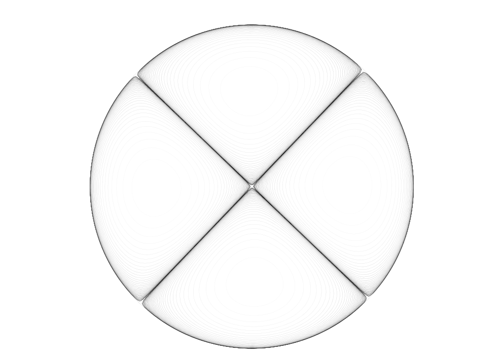
Refer to caption
Figure 1. Optimal partition and eigenfunctions for (1.5).

On the left of Figure 1 is a representation of the eigenfunctions associated to the first eigenvalues of the partition: they highlight the two sets of the partition, which are symmetric semicircles. On the right the second eigenfunctions of the two sets. Observe the additional nodal lines (in connected sets the second eigenfunctions is sign-changing). In this case the strong symmetry of the two functionals seems to translate in the symmetry of their solutions.

In Figure 2, a numerical approximation for

(ω1,ω2)↦λ1​(ω1)​λ2​(ω1)+λ1​(ω2)2+λ2​(ω2)2.(\omega_{1},\omega_{2})\mapsto\lambda_{1}(\omega_{1})\lambda_{2}(\omega_{1})+\lambda_{1}(\omega_{2})^{2}+\lambda_{2}(\omega_{2})^{2}. (1.6)

In this case the functional is no more symmetric and the solution too looses symmetry. Nevertheless, observe that the cost functional is scale-invariant.

Refer to caption
Refer to caption
Figure 2. Optimal partition and eigenfunctions for (1.6).

On the left of Figure 2 is a representation of the eigenfunctions associated to the first eigenvalues of the partition and the two sets ω1\omega_{1} (in the center) and ω2\omega_{2} (the two lobes). On the right the second eigenfunctions of the two sets. Observe that the second domain is not connected and, numerically, it holds λ1​(ω2)=λ2​(ω2)\lambda_{1}(\omega_{2})=\lambda_{2}(\omega_{2}). This implies that the first eigenvalue of the second subset of the partition has multiplicity two and one can choose the corresponding eigenfunction to have disjoint supports contained in only one of the two lobes at the time. This suggests that there are minimal partitions made of disconnected sets and were the eigenvalues have multiplicity higher than one (unlike the case of cost functions depending on first eigenvalues only). Any choice of eigenfunctions will still verify (1.4) with the same coefficients. Finally we point out that in this example the equi-partition of angles at singular points seems false (unlike in [17]), although at the moment we lack any explicit counterexample of this fact.

In Figure 3, a numerical approximation of the optimal partition of the unit ball associated to

(ω1,ω2)↦(λ1​(ω1)20+λ2​(ω1)20+λ1​(ω2)20)1/20.(\omega_{1},\omega_{2})\mapsto\left(\lambda_{1}(\omega_{1})^{20}+\lambda_{2}(\omega_{1})^{20}+\lambda_{1}(\omega_{2})^{20}\right)^{1/20}. (1.7)

This functional gives a rather good approximation of the cost

(ω1,ω2)↦max⁡(λ2​(ω1),λ1​(ω2))(\omega_{1},\omega_{2})\mapsto\mathrm{max}\left(\lambda_{2}(\omega_{1}),\lambda_{1}(\omega_{2})\right)

which does not fall in the scope of our main result, as it is not strictly monotone with respect to λ1​(ω1)\lambda_{1}(\omega_{1}). It can be shown that the optimal partition corresponding to this last function is the two third sector of the circle (ω1\omega_{1}) and a third sector of the circle (ω2\omega_{2}). We obtain a rather similar result for (1.7).

Figure 3. Optimal partition and eigenfunctions for (1.7). We observe some numerical artifact in the first picture: the presence of a region where the eigenfunctions are zero. This points out a weakness of our numerical scheme when some of the coefficients in (1.4) are small compared to the others.

On the left the eigenfunctions associated to the first eigenvalues of the partition and on the right the second eigenfunction of the first subset. We point out a seemingly singular point at the center of the ball. According to Theorem 1.1 all the eigenfunctions in the energy functional are regular, and indeed the first eigenfunction of ω1\omega_{1} is regular, but it appears that as the exponent in the functional becomes larger and larger (the lpl^{p} norm approaches the l∞l^{\infty} norm), the first eigenfunctions loses its regularity. This phenomenon will be the object of an upcoming paper.

2. The penalization argument: an approximate problem

In order to simplify the presentation, we only detail the proof in the case m=2m=2, k1=k2=:k∈ℕk_{1}=k_{2}=:k\in\mathbb{N} and φ1=φ2=:φ\varphi_{1}=\varphi_{2}=:\varphi. The general case follows by the same argument with some simple modifications. In this particular situation, problem (1.3) becomes

c~=inf(ω1,ω2)∈𝒫~2​(Ω)F⁡(φ⁡(λ~1​(ω1),…,λ~k​(ω1)),φ⁡(λ~1​(ω2),…,λ~k​(ω2)))\widetilde{c}=\inf_{(\omega_{1},\omega_{2})\in\widetilde{\mathcal{P}}_{2}(\Omega)}F\left(\varphi(\widetilde{\lambda}_{1}(\omega_{1}),\ldots,\widetilde{\lambda}_{k}(\omega_{1})),\varphi(\widetilde{\lambda}_{1}(\omega_{2}),\ldots,\widetilde{\lambda}_{k}(\omega_{2}))\right) (2.1)

where, we recall,

𝒫~2(Ω)={(ω1,ω2)⊆Ω×Ω:ω1,ω2 measurable, |ω1∩ω2|=0}.\widetilde{\mathcal{P}}_{2}(\Omega)=\left\{(\omega_{1},\omega_{2})\subseteq\Omega\times\Omega:\ \omega_{1},\omega_{2}\text{ measurable, }|\omega_{1}\cap\omega_{2}|=0\right\}.

Following [20], this problem has at least one open and regular solution in the sense of Theorem 1.1. Here we show that every solution of this problem is equivalent to an open and regular partition, together with some regularity properties of the associated eigenfunctions and a free boundary condition (1.1).

Keeping this in mind, let (ω1,ω2)∈𝒫~2​(Ω)(\omega_{1},\omega_{2})\in\widetilde{\mathcal{P}}_{2}(\Omega) be a solution of (2.1). We denote by {(λ~i​(ω1),ϕi)}i∈ℕ\{(\widetilde{\lambda}_{i}(\omega_{1}),\phi_{i})\}_{i\in\mathbb{N}} and {(λ~i​(ω2),ψi)}i∈ℕ\{(\widetilde{\lambda}_{i}(\omega_{2}),\psi_{i})\}_{i\in\mathbb{N}} the sequences of nondecreasing generalized eigenvalues (enumerated with multiplicity) and corresponding orthonormal eigenfunctions of the Laplacian in H~01​(ω1)\widetilde{H}^{1}_{0}(\omega_{1}) and H~01​(ω2)\widetilde{H}^{1}_{0}(\omega_{2}), respectively. We point out that, even though the eigenfunctions associated to the generalized eigenvalues belong to some Sobolev-like spaces, they are still H01​(Ω)H^{1}_{0}(\Omega) functions. Thus we have the identities

∫Ωϕi​ϕj=δi​j,and∫Ω∇ϕi⋅∇ϕj=λ~i​(ω1)​δi​j,\int_{\Omega}\phi_{i}\phi_{j}=\delta_{ij},\quad\text{and}\quad\int_{\Omega}\nabla\phi_{i}\cdot\nabla\phi_{j}=\widetilde{\lambda}_{i}(\omega_{1})\delta_{ij},

and similarly for {ψi}i∈ℕ\{\psi_{i}\}_{i\in\mathbb{N}}. Here δi​j\delta_{ij} denotes the Kronecker symbol, that is δi​j=1\delta_{ij}=1 if i=ji=j and 00 otherwise.

Remark 2.1.

We point out that, a priori, the sets span⁡{ϕ1,…,ϕk}\mathrm{span}\{\phi_{1},\ldots,\phi_{k}\} and span⁡{ψ1,…,ψk}\mathrm{span}\{\psi_{1},\ldots,\psi_{k}\} may not contain all the eigenfunctions associated to λ~k​(ω1)\widetilde{\lambda}_{k}(\omega_{1}) and λ~k​(ω2)\widetilde{\lambda}_{k}(\omega_{2}). However, we shall see later on that this is never the case, thanks to the spectral gap property (cfr. Theorem 1.1).

We denote ϕ=(ϕ1,…,ϕk)\bm{\phi}=(\phi_{1},\ldots,\phi_{k}) and 𝝍=(ψ1,…,ψk)\bm{\psi}=(\psi_{1},\ldots,\psi_{k}) and we introduce two linear subspaces of L2​(Ω)L^{2}(\Omega) generated by ϕ\bm{\phi} adn 𝝍\bm{\psi}, together with their orthogonal projections:

L⁡(ϕ)=span⁡{ϕ1,…,ϕk},P⟂:L2​(Ω)→L​(ϕ)⟂,\displaystyle L(\bm{\phi})=\mathrm{span}\left\{\phi_{1},\ldots,\phi_{k}\right\},\qquad P^{\perp}:L^{2}(\Omega)\to L(\bm{\phi})^{\perp},
L⁡(𝝍)=span⁡{ψ1,…,ψk},Q⟂:L2​(Ω)→L​(𝝍)⟂.\displaystyle L(\bm{\psi})=\mathrm{span}\left\{\psi_{1},\ldots,\psi_{k}\right\},\qquad Q^{\perp}:L^{2}(\Omega)\to L(\bm{\psi})^{\perp}.

Exploiting the orthogonality of ϕ\bm{\phi} and ϕ\bm{\phi} we find that for every w∈L2​(Ω)w\in L^{2}(\Omega) the projections are

P⟂​w=w−∑i=1k⟨w,ϕi⟩L2​(Ω)andQ⟂​w=w−∑i=1k⟨w,ψi⟩L2​(Ω).P^{\perp}w=w-\sum_{i=1}^{k}\langle w,\phi_{i}\rangle_{L^{2}(\Omega)}\qquad\text{and}\qquad Q^{\perp}w=w-\sum_{i=1}^{k}\langle w,\psi_{i}\rangle_{L^{2}(\Omega)}.

where ⟨⋅,⋅⟩L2​(Ω)\langle\cdot,\cdot\rangle_{L^{2}(\Omega)} denotes the usual scalar product in L2​(Ω)L^{2}(\Omega).

Our aim is to define an energy functional and an associated minimization problem whose solutions are close to those of (2.1). In order to achieve this, we need to introduce a regularized energy functional with two additional terms. For the first one, inspired by [20], we relax the disjointedness constraint of the supports of the eigenfunctions ϕ\bm{\phi} and 𝝍\bm{\psi} by introducing a competition term between groups of eigenfunctions; this allows to prove the regularity of both the partition and of the eigenfunctions. For the second one, using the projection operators P⟂P^{\perp} and Q⟂Q^{\perp}, we introduce a penalization that enables us to select the specific minimizer to which the sequence of approximated minimizers converges. This allows to prove that the singular limits are, up to orthogonal transformation, the original eigenfunctions. We need a couple of technical tools before introducing the approximating functionals.

Given 𝐮,𝐯∈H01​(Ω,ℝk)\mathbf{u},\mathbf{v}\in H^{1}_{0}(\Omega;\mathbb{R}^{k}), define the k×kk\times k symmetric and positive definite matrices

M⁡(𝐮):=(∫Ω∇ui⋅∇uj+(P⟂​ui)​(P⟂​uj))i,j=(⟨∇ui,∇uj⟩L2​(Ω)+⟨P⟂​ui,P⟂​uj⟩L2​(Ω))i,j,N⁡(𝐯):=(∫Ω∇vi⋅∇vj+(Q⟂​vi)​(Q⟂​vj))i,j=(⟨∇vi,∇vj⟩L2​(Ω)+⟨Q⟂​vi,Q⟂​vj⟩L2​(Ω))i,j.\begin{split}M(\mathbf{u}):=&\left(\int_{\Omega}\nabla u_{i}\cdot\nabla u_{j}\,+(P^{\perp}u_{i})(P^{\perp}u_{j})\right)_{i,j}=\left(\langle\nabla u_{i},\nabla u_{j}\rangle_{L^{2}(\Omega)}+\langle P^{\perp}u_{i},P^{\perp}u_{j}\rangle_{L^{2}(\Omega)}\right)_{i,j},\\ N(\mathbf{v}):=&\left(\int_{\Omega}\nabla v_{i}\cdot\nabla v_{j}\,+(Q^{\perp}v_{i})(Q^{\perp}v_{j})\right)_{i,j}=\left(\langle\nabla v_{i},\nabla v_{j}\rangle_{L^{2}(\Omega)}+\langle Q^{\perp}v_{i},Q^{\perp}v_{j}\rangle_{L^{2}(\Omega)}\right)_{i,j}.\end{split}

Observe that for any orthogonal matrix O∈𝒪k​(ℝ)O\in\mathcal{O}_{k}(\mathbb{R}) we have

M⁡(O​𝐮)=O​M​(𝐮)​OT,N⁡(O​𝐯)=O​N​(𝐯)​OT.M(O\mathbf{u})=OM(\mathbf{u})O^{T},\qquad N(O\mathbf{v})=ON(\mathbf{v})O^{T}.

In particular M⁡(O​𝐮)M(O\mathbf{u}) and M⁡(𝐮)M(\mathbf{u}) have the same spectrum.

We extend the function φ:(ℝ+)k→ℝ\varphi:(\mathbb{R}^{+})^{k}\to\mathbb{R} to the set of symmetric and positive definite matrices in the following way: given such a matrix MM, we let

φ⁡(M)=φ⁡(γ1,…,γk),\varphi(M)=\varphi(\gamma_{1},\ldots,\gamma_{k}),

where γ1,…,γk\gamma_{1},\dots,\gamma_{k} are the (positive) eigenvalues of MM (with an abuse of notation, we identify the function acting on the eigenvalues with the function acting on the matrices). Observe that such function is well defined by the symmetry assumption (H3). By definition, we have

φ⁡(O​M​OT)=φ⁡(M) for every M symmetric positive definite, O∈𝒪k​(ℝ)\varphi(OMO^{T})=\varphi(M)\qquad\text{ for every $M$ symmetric positive definite, $O\in\mathcal{O}_{k}(\mathbb{R})$}

Since the original function (acting on the eigenvalues) is smooth and symmetric, we find that φ\varphi is also a C1C^{1} function in the set of symmetric and positive definite matrices. We denote

∂∂Ei​j​φ​(M)=limh→0φ⁡(M+h⁡(Ei​j+Ej​i)/2)−φ⁡(M)h\frac{\partial}{\partial E_{ij}}\varphi(M)=\lim_{h\to 0}\frac{\varphi(M+h(E_{ij}+E_{ji})/2)-\varphi(M)}{h}

the (tangent) derivative, in the set of symmetric matrices, of φ\varphi at MM with respect to the component (i,j)(i,j). Here Ei​jE_{ij} is the matrix whose component (i,j)(i,j) is equal to 11, while all other components are 00.

Example 2.2.

In some notable cases the extended functions can be computed explicitly. For the map (s1,…,sk)↦(∑i=1k(si)p)1/p(s_{1},\ldots,s_{k})\mapsto\left(\sum_{i=1}^{k}(s_{i})^{p}\right)^{1/p}, we have φ⁡(M):=(∑i=1k(γi)p)1/p=(trace​(Mp))1/p\varphi(M):=\left(\sum_{i=1}^{k}(\gamma_{i})^{p}\right)^{1/p}=\left(\textrm{trace}(M^{p})\right)^{1/p}, which coincides with the pp-Schatten norm of a symmetric and positive definite matrix MM. For (s1,…,sk)↦∏i=1ksi(s_{1},\ldots,s_{k})\mapsto\prod_{i=1}^{k}s_{i}, we have φ⁡(M):=∏i=1kγi=det(M)\varphi(M):=\prod_{i=1}^{k}\gamma_{i}=\det(M). These examples are related to 1.1.

Lemma 2.3 ([20, Lemma 3.6]).

For every diagonal matrix D=diag(γ1,…,γk)D=\diag(\gamma_{1},\ldots,\gamma_{k}), we have

∂∂Ei​i​φ​(D)=∂iφ⁡(γ1,…,γk)∀i,∂∂Ei​j​φ​(D)=0∀i≠j.\frac{\partial}{\partial E_{ii}}\varphi(D)=\partial_{i}\varphi(\gamma_{1},\ldots,\gamma_{k})\quad\forall i,\qquad\frac{\partial}{\partial E_{ij}}\varphi(D)=0\quad\forall i\neq j.

We are now ready to introduce the family of approximating functionals. Fix any exponent 1/2<q<2∗/4=N/[2​(N−2)+]1/2<q<2^{*}/4=N/[2(N-2)^{+}]. For β>0\beta>0 we define the C1C^{1} energy functional Eβ:H01​(Ω,ℝk)×H01​(Ω,ℝk)→ℝE_{\beta}:H^{1}_{0}(\Omega,\mathbb{R}^{k})\times H^{1}_{0}(\Omega,\mathbb{R}^{k})\to\mathbb{R} as

Eβ​(𝐮,𝐯)=F⁡(φ⁡(M⁡(𝐮)),φ⁡(N⁡(𝐯)))+βq​∫Ω(∑i=1kui2)q​(∑i=1kvi2)q\displaystyle E_{\beta}(\mathbf{u},\mathbf{v})=F\left(\varphi(M(\mathbf{u})),\varphi(N(\mathbf{v}))\right)+\frac{\beta}{q}\int_{\Omega}\Big(\sum_{i=1}^{k}u_{i}^{2}\Big)^{q}\Big(\sum_{i=1}^{k}v_{i}^{2}\Big)^{q}

and the least energy level

cβ:=inf{Eβ(𝐮,𝐯):𝐮,𝐯∈Σ(L2)},c_{\beta}:=\inf\left\{E_{\beta}(\mathbf{u},\mathbf{v}):\mathbf{u},\mathbf{v}\in\Sigma(L^{2})\right\}, (2.2)

where

Σ(L2):={𝐰=(w1,…,wk)∈H01(Ω;ℝk):∫Ωwiwj=δi​j for every i,j}.\Sigma(L^{2}):=\left\{\mathbf{w}=(w_{1},\ldots,w_{k})\in H^{1}_{0}(\Omega;\mathbb{R}^{k}):\ \int_{\Omega}w_{i}w_{j}=\delta_{ij}\text{ for every }i,j\right\}.

The functional and the set Σ⁡(L2)\Sigma(L^{2}) are invariant under multiplication by orthogonal matrices

Eβ​(𝐮,𝐯)=Eβ​(O1​𝐮,O2​𝐯)∀O1,O2∈𝒪k​(ℝ),E_{\beta}(\mathbf{u},\mathbf{v})=E_{\beta}(O_{1}\mathbf{u},O_{2}\mathbf{v})\qquad\forall O_{1},O_{2}\in\mathcal{O}_{k}(\mathbb{R}),

and

(𝐮,𝐯)∈Σ⁡(L2)⇔(O1​𝐮,O2​𝐯)∈Σ⁡(L2),∀O1,O2∈𝒪k​(ℝ).(\mathbf{u},\mathbf{v})\in\Sigma(L^{2})\iff(O_{1}\mathbf{u},O_{2}\mathbf{v})\in\Sigma(L^{2}),\;\forall O_{1},O_{2}\in\mathcal{O}_{k}(\mathbb{R}).

One should keep in mind that EβE_{\beta} and cβc_{\beta} also depend on the vectors of eigenfunctions ϕ\bm{\phi}, 𝝍\bm{\psi}. However, in order to simplify the notation, we will not point out this dependence explicitly.

Lemma 2.4.

For each β>0\beta>0 we have

F⁡(φ⁡(M⁡(𝐮),φ⁡(N⁡(𝐯)))≥F⁡(φ⁡(λ1​(Ω),λk​(Ω)),…,φ⁡(λ1​(Ω),…,λk​(Ω)))∀𝐮,𝐯∈Σ⁡(L2)CLOSEF(\varphi(M(\mathbf{u}),\varphi(N(\mathbf{v})))\geq F(\varphi(\lambda_{1}(\Omega),\lambda_{k}(\Omega)),\ldots,\varphi(\lambda_{1}(\Omega),\ldots,\lambda_{k}(\Omega)))\qquad\forall\mathbf{u},\mathbf{v}\in\Sigma(L^{2})

and cβc_{\beta} is finite.

Proof.

For any (𝐮,𝐯)∈Σ⁡(L2)(\mathbf{u},\mathbf{v})\in\Sigma(L^{2}), take O1,O2∈𝒪k​(ℝ)O_{1},O_{2}\in\mathcal{O}_{k}(\mathbb{R}) in such a way that O1​M​(𝐮)​O1TO_{1}M(\mathbf{u})O_{1}^{T}, O2​N​(𝐯)​O2TO_{2}N(\mathbf{v})O_{2}^{T} are diagonal and the elements on the diagonal are ordered nondecreasingly. Let 𝐮~=O1​𝐮\mathbf{\widetilde{u}}=O_{1}\mathbf{u}, 𝐯~=O2​𝐯\mathbf{\widetilde{v}}=O_{2}\mathbf{v}. Exploiting the monotonicity of FF and φ\varphi, and the invariance of Σ⁡(L2)\Sigma(L^{2}) and φ\varphi under orthogonal transformations, we find that

F⁡(φ⁡(M⁡(𝐮),φ⁡(N⁡(𝐯)))CLOSE\displaystyle F(\varphi(M(\mathbf{u}),\varphi(N(\mathbf{v}))) =F⁡(φ⁡(M⁡(𝐮~),φ⁡(N⁡(𝐯~)))CLOSE\displaystyle=F(\varphi(M(\mathbf{\widetilde{u}}),\varphi(N(\mathbf{\widetilde{v}})))
=F⁡(φ⁡(∫Ω|∇u~1|2+(P⟂​u~1)2,…,∫Ω|∇u~k|2+(P⟂​u~k)2)CLOSE,\displaystyle=F\left(\varphi\left(\int_{\Omega}|\nabla\widetilde{u}_{1}|^{2}+(P^{\perp}\widetilde{u}_{1})^{2},\ldots,\int_{\Omega}|\nabla\widetilde{u}_{k}|^{2}+(P^{\perp}\widetilde{u}_{k})^{2}\right),\right.
OPENφ⁡(∫Ω|∇v~1|2+(Q⟂​v~1)2,…,∫Ω|∇v~k|2+(Q⟂​v~k)2))\displaystyle\phantom{=F(\varphi(\int}\left.\varphi\left(\int_{\Omega}|\nabla\widetilde{v}_{1}|^{2}+(Q^{\perp}\widetilde{v}_{1})^{2},\ldots,\int_{\Omega}|\nabla\widetilde{v}_{k}|^{2}+(Q^{\perp}\widetilde{v}_{k})^{2}\right)\right)
≥F⁡(φ⁡(λ1​(Ω),…,λk​(Ω)),…,φ⁡(λ1​(Ω),…,λk​(Ω)))\displaystyle\geq F(\varphi(\lambda_{1}(\Omega),\ldots,\lambda_{k}(\Omega)),\ldots,\varphi(\lambda_{1}(\Omega),\ldots,\lambda_{k}(\Omega)))

Then, recalling that β>0\beta>0, we conclude

cβ≥F⁡(φ⁡(λ1​(Ω),…,λk​(Ω)),…,φ⁡(λ1​(Ω),…,λk​(Ω)))>−∞.∎c_{\beta}\geq F(\varphi(\lambda_{1}(\Omega),\ldots,\lambda_{k}(\Omega)),\ldots,\varphi(\lambda_{1}(\Omega),\ldots,\lambda_{k}(\Omega)))>-\infty.\qed

We have established that for any β>0\beta>0, the functional EβE_{\beta} is bounded from below in Σ⁡(L2)\Sigma(L^{2}). We now show that the infimum is always attained, making the least energy level cβc_{\beta} in (2.2) a critical level for EβE_{\beta}. For notation convenience, let

Gβ={(𝐮,𝐯)∈Σ⁡(L2):Eβ​(𝐮,𝐯)=cβ}.G_{\beta}=\{(\mathbf{u},\mathbf{v})\in\Sigma(L^{2}):E_{\beta}(\mathbf{u},\mathbf{v})=c_{\beta}\}.
Proposition 2.5.

For any β>0\beta>0, we have the following:

  1. (a)

    the value cβc_{\beta} is a critical level for the functional EβE_{\beta} and GβG_{\beta} is not empty. Moreover, for every (𝐮,𝐯)=((u1,…,uk),(v1,…,vk))∈Mβ(\mathbf{u},\mathbf{v})=((u_{1},\ldots,u_{k}),(v_{1},\ldots,v_{k}))\in M_{\beta}, we have

    Eβ′​(𝐮,𝐯)=0.E^{\prime}_{\beta}(\mathbf{u},\mathbf{v})=0.
  2. (b)

    For any O1,O2∈𝒪k​(ℝ)O_{1},O_{2}\in\mathcal{O}_{k}(\mathbb{R}) orthogonal matrices,

    (𝐮,𝐯)∈Gβ⟹(O1​𝐮,O2​𝐯)∈Gβ.(\mathbf{u},\mathbf{v})\in G_{\beta}\implies(O_{1}\mathbf{u},O_{2}\mathbf{v})\in G_{\beta}.

    Therefore, if (𝐮,𝐯)∈Gβ(\mathbf{u},\mathbf{v})\in G_{\beta} we can further assume that it verifies

    ∫Ω∇ui⋅∇uj+(P⟂​ui)​(P⟂​uj)\displaystyle\int_{\Omega}\nabla u_{i}\cdot\nabla u_{j}+(P^{\perp}u_{i})(P^{\perp}u_{j}) =∫Ω∇vi⋅∇vj+(Q⟂​vi)​(Q⟂​vj)=0\displaystyle=\int_{\Omega}\nabla v_{i}\cdot\nabla v_{j}+(Q^{\perp}v_{i})(Q^{\perp}v_{j})=0 ∀i≠j\displaystyle\forall i\neq j (2.3)
    ∫Ω|∇ui|2+(P⟂​ui)2≤∫Ω|∇uj|2+(P⟂​uj)2\displaystyle\int_{\Omega}|\nabla u_{i}|^{2}+(P^{\perp}u_{i})^{2}\leq\int_{\Omega}|\nabla u_{j}|^{2}+(P^{\perp}u_{j})^{2} ,∫Ω|∇vi|2+(Q⟂vi)2≤∫Ω|∇vj|2+(Q⟂vj)2\displaystyle,\;\int_{\Omega}|\nabla v_{i}|^{2}+(Q^{\perp}v_{i})^{2}\leq\int_{\Omega}|\nabla v_{j}|^{2}+(Q^{\perp}v_{j})^{2} ∀i≤j.\displaystyle\forall i\leq j. (2.4)

    In particular, M⁡(𝐮),N⁡(𝐯)M(\mathbf{u}),N(\mathbf{v}) are orthogonal matrices, and

    Eβ(𝐮,𝐯)=F(φ(∫Ω|∇u1|2+(P⟂u1)2,…,∫Ω|∇uk|2+(P⟂uk)2),OPENφ⁡(∫Ω|∇v1|2+(P⟂​v1)2,…,∫Ω|∇vk|2+(P⟂​vk)2))+βq∫Ω(∑j=1kui2)q(∑i=1kvi2)q.E_{\beta}(\mathbf{u},\mathbf{v})=F\left(\varphi\left(\int_{\Omega}|\nabla u_{1}|^{2}+(P^{\perp}u_{1})^{2},\ldots,\int_{\Omega}|\nabla u_{k}|^{2}+(P^{\perp}u_{k})^{2}\right),\right.\\ \left.\varphi\left(\int_{\Omega}|\nabla v_{1}|^{2}+(P^{\perp}v_{1})^{2},\ldots,\int_{\Omega}|\nabla v_{k}|^{2}+(P^{\perp}v_{k})^{2}\right)\right)\\ +\frac{\beta}{q}\int_{\Omega}\Big(\sum_{j=1}^{k}u_{i}^{2}\Big)^{q}\Big(\sum_{i=1}^{k}v_{i}^{2}\Big)^{q}.
  3. (c)

    For i,j=1,…,ki,j=1,\dots,k there exist Lagrange multipliers μi​j,β,νi​j,β>0\mu_{ij,\beta},\nu_{ij,\beta}>0, and coefficients

    ai,β\displaystyle a_{i,\beta} =∂1F⁡(φ⁡(M⁡(𝐮)),φ⁡(N⁡(𝐯)))⋅∂iφ⁡(∫Ω|∇u1|2+(P⟂​u1)2,…,∫Ω|∇uk|2+(P⟂​uk)2)>0\displaystyle=\partial_{1}F\left(\varphi(M(\mathbf{u})),\varphi(N(\mathbf{v}))\right)\cdot\partial_{i}\varphi\left(\int_{\Omega}|\nabla u_{1}|^{2}+(P^{\perp}u_{1})^{2},\ldots,\int_{\Omega}|\nabla u_{k}|^{2}+(P^{\perp}u_{k})^{2}\right)>0 (2.5)
    bi,β\displaystyle b_{i,\beta} =∂2F⁡(φ⁡(M⁡(𝐮)),φ⁡(N⁡(𝐯)))⋅∂iφ⁡(∫Ω|∇v1|2+(Q⟂​v1)2,…,∫Ω|∇vk|2+(Q⟂​vk)2)>0\displaystyle=\partial_{2}F\left(\varphi(M(\mathbf{u})),\varphi(N(\mathbf{v}))\right)\cdot\partial_{i}\varphi\left(\int_{\Omega}|\nabla v_{1}|^{2}+(Q^{\perp}v_{1})^{2},\ldots,\int_{\Omega}|\nabla v_{k}|^{2}+(Q^{\perp}v_{k})^{2}\right)>0

    such that the components of (𝐮,𝐯)(\mathbf{u},\mathbf{v}) solve the system

    {ai,β​(−Δ​ui+P⟂​ui)=∑j=1kμi​j,β​uj−β​ui​(∑j=1kuj2)q−1​(∑j=1kvj2)qbi,β​(−Δ​vi+Q⟂​vi)=∑j=1kνi​j,β​vj−β​vi​(∑j=1kvj2)q−1​(∑j=1kuj2)q in ​Ω.\begin{cases}a_{i,\beta}(-\Delta u_{i}+P^{\perp}u_{i})=\sum_{j=1}^{k}\mu_{ij,\beta}u_{j}-\beta u_{i}\left(\sum_{j=1}^{k}u_{j}^{2}\right)^{q-1}\left(\sum_{j=1}^{k}v_{j}^{2}\right)^{q}\\[10.0pt] b_{i,\beta}(-\Delta v_{i}+Q^{\perp}v_{i})=\sum_{j=1}^{k}\nu_{ij,\beta}v_{j}-\beta v_{i}\left(\sum_{j=1}^{k}v_{j}^{2}\right)^{q-1}\left(\sum_{j=1}^{k}u_{j}^{2}\right)^{q}\end{cases}\quad\text{ in }\Omega. (2.6)

In view of the previous result, whenever we refer to GβG_{\beta} we assume that its functions verify the additional conditions (2.3) and (2.4).

Proof.

The result follows by the critical point theory of functionals in Hilbert spaces. First, some preliminary remarks :

  1. (1)

    Σ⁡(L2)\Sigma(L^{2}) is a C1C^{1} submanifold of H01​(Ω,ℝk)H^{1}_{0}(\Omega,\mathbb{R}^{k}) of codimension k⁡(k+1)/2k(k+1)/2 (see [20, Lemma 3.7]).

  2. (2)

    Eβ:H01​(Ω)×H01​(Ω)→ℝ+E_{\beta}:H^{1}_{0}(\Omega)\times H^{1}_{0}(\Omega)\to\mathbb{R}^{+} is a C1C^{1} functional and, for any 𝝃,𝜼∈H01​(Ω,ℝk)\bm{\xi},\bm{\eta}\in H^{1}_{0}(\Omega,\mathbb{R}^{k}), we have

    Eβ′​(𝐮,𝐯)​(𝝃,𝜼)2=\displaystyle\frac{E_{\beta}^{\prime}(\mathbf{u},\mathbf{v})(\bm{\xi},\bm{\eta})}{2}= ∂1F⁡(φ⁡(M⁡(𝐮)),φ⁡(N⁡(𝐯)))​∑i≤jk∂∂Ei​j​φ​(M⁡(𝐮))​∫Ω(∇ui⋅∇ξj+(P⟂​ui)​ξj)\displaystyle\partial_{1}F\left(\varphi(M(\mathbf{u})),\varphi(N(\mathbf{v}))\right)\sum_{i\leq j}^{k}\frac{\partial}{\partial E_{ij}}\varphi(M(\mathbf{u}))\int_{\Omega}(\nabla u_{i}\cdot\nabla\xi_{j}+(P^{\perp}u_{i})\xi_{j})
    +∂2F(φ(M(𝐮)),φ(N(𝐯)))∑i≤jk∂∂Ei​jφ(N(𝐯))∫Ω(∇vi⋅∇ηj+(Q⟂vj)ηj)\displaystyle+\partial_{2}F\left(\varphi(M(\mathbf{u})),\varphi(N(\mathbf{v}))\right)\sum_{i\leq j}^{k}\frac{\partial}{\partial E_{ij}}\varphi(N(\mathbf{v}))\int_{\Omega}(\nabla v_{i}\cdot\nabla\eta_{j}+(Q^{\perp}v_{j})\eta_{j})
    +β∑i=1k∫Ωuiξi(∑j=1kui2)q−1(∑i=1kvi2)q+β∑i=1k∫Ωviηi(∑j=1kvi2)q−1(∑i=1kui2)q.\displaystyle+\beta\sum_{i=1}^{k}\int_{\Omega}u_{i}\xi_{i}\Big(\sum_{j=1}^{k}u_{i}^{2}\Big)^{q-1}\Big(\sum_{i=1}^{k}v_{i}^{2}\Big)^{q}+\beta\sum_{i=1}^{k}\int_{\Omega}v_{i}\eta_{i}\Big(\sum_{j=1}^{k}v_{i}^{2}\Big)^{q-1}\Big(\sum_{i=1}^{k}u_{i}^{2}\Big)^{q}.

Let β>0\beta>0. By Lemma 2.4 we have cβ>−∞c_{\beta}>-\infty. We take a minimizing sequence 𝐮n=(u1,n,…,uk,n)\mathbf{u}_{n}=(u_{1,n},\ldots,u_{k,n}), 𝐯n=(v1,n,…,vk,n)∈Σ⁡(L2)\mathbf{v}_{n}=(v_{1,n},\ldots,v_{k,n})\in\Sigma(L^{2}), Eβ​(𝐮n,𝐯n)→cβE_{\beta}(\mathbf{u}_{n},\mathbf{v}_{n})\to c_{\beta} as n→∞n\to\infty. By Ekeland’s Variational Principle and by property (1) listed above, we can suppose without loss of generality that Eβ|Σ⁡(L2)′​(𝐮n,𝐯n)→0E_{\beta}|_{\Sigma(L^{2})}^{\prime}(\mathbf{u}_{n},\mathbf{v}_{n})\to 0 in H−1​(Ω,ℝk)H^{-1}(\Omega,\mathbb{R}^{k}). For each n∈ℕn\in\mathbb{N} take O1,n,O2,n∈𝒪k​(ℝ)O_{1,n},O_{2,n}\in\mathcal{O}_{k}(\mathbb{R}) such that O1,n​M​(𝐮n)​O1,nTO_{1,n}M(\mathbf{u}_{n})O_{1,n}^{T} and O2,n​M​(𝐯n)​O2,nTO_{2,n}M(\mathbf{v}_{n})O_{2,n}^{T} are diagonal matrices and let

𝐮~n:=O1,n​𝐮nand𝐯~n:=O2,n​𝐯.\mathbf{\widetilde{u}}_{n}:=O_{1,n}\mathbf{u}_{n}\quad\text{and}\quad\mathbf{\widetilde{v}}_{n}:=O_{2,n}\mathbf{v}.

Then Eβ​(𝐮~n,𝐯~n)=Eβ​(𝐮n,𝐯n)E_{\beta}(\mathbf{\widetilde{u}}_{n},\mathbf{\widetilde{v}}_{n})=E_{\beta}(\mathbf{u}_{n},\mathbf{v}_{n}), 𝐮~n,𝐯~n∈Σ⁡(L2)\mathbf{\widetilde{u}}_{n},\mathbf{\widetilde{v}}_{n}\in\Sigma(L^{2}) and

Eβ​(𝐮~n,𝐯~n)→cβ,Eβ′|Σ⁡(L2)​(𝐮~n,𝐯~n)→0 as ​n→∞.E_{\beta}(\mathbf{\widetilde{u}}_{n},\mathbf{\widetilde{v}}_{n})\to c_{\beta},\qquad E_{\beta}^{\prime}|_{\Sigma(L^{2})}(\mathbf{\widetilde{u}}_{n},\mathbf{\widetilde{v}}_{n})\to 0\quad\text{ as }n\to\infty.

Therefore

F(φ(∫Ω|∇u~1,n|2+(P⟂u~1,n)2,…,∫Ω|∇u~k,n|2+(P⟂u~k,n)2),OPENφ⁡(∫Ω|∇v~1,n|2+(P⟂​v~1,n)2,…,∫Ω|∇v~k,n|2+(P⟂​v~k,n)2))≤Eβ​(𝐮~n,𝐯~n)≤cβ+1F\left(\varphi\left(\int_{\Omega}|\nabla\widetilde{u}_{1,n}|^{2}+(P^{\perp}\widetilde{u}_{1,n})^{2},\ldots,\int_{\Omega}|\nabla\widetilde{u}_{k,n}|^{2}+(P^{\perp}\widetilde{u}_{k,n})^{2}\right),\right.\\ \left.\varphi\left(\int_{\Omega}|\nabla\widetilde{v}_{1,n}|^{2}+(P^{\perp}\widetilde{v}_{1,n})^{2},\ldots,\int_{\Omega}|\nabla\widetilde{v}_{k,n}|^{2}+(P^{\perp}\widetilde{v}_{k,n})^{2}\right)\right)\leq E_{\beta}(\mathbf{\widetilde{u}}_{n},\mathbf{\widetilde{v}}_{n})\leq c_{\beta}+1

for large nn. Since 𝐮~n,𝐯~n∈Σ⁡(L2)\mathbf{\widetilde{u}}_{n},\mathbf{\widetilde{v}}_{n}\in\Sigma(L^{2}) then

λ1​(Ω)≤∫Ω|∇u~i,n|2,∫Ω|∇v~i,n|2.\lambda_{1}(\Omega)\leq\int_{\Omega}|\nabla\widetilde{u}_{i,n}|^{2},\int_{\Omega}|\nabla\widetilde{v}_{i,n}|^{2}.

Combining this information with (H1)–(H2) we deduce that 𝐮~n,𝐯~n\mathbf{\widetilde{u}}_{n},\mathbf{\widetilde{v}}_{n} are bounded sequences in H01​(Ω,ℝk)H^{1}_{0}(\Omega,\mathbb{R}^{k}), so that (up to subsequence) 𝐮~n⇀𝐮~\mathbf{\widetilde{u}}_{n}\rightharpoonup\mathbf{\widetilde{u}}, 𝐯~n⇀𝐯~\mathbf{\widetilde{v}}_{n}\rightharpoonup\mathbf{\widetilde{v}} weakly in H01​(Ω,ℝk)H^{1}_{0}(\Omega,\mathbb{R}^{k}), strongly in Lr​(Ω,ℝk)L^{r}(\Omega;\mathbb{R}^{k}), for every 1≤r<2∗1\leq r<2^{*}. We can now conclude exactly as in [20, Theorem 3.8], observing that ∂∂Ei​j​φ​(M⁡(𝐮~n))=∂∂Ei​j​φ​(N⁡(𝐯~n))=0\frac{\partial}{\partial E_{ij}}\varphi(M(\mathbf{\widetilde{u}}_{n}))=\frac{\partial}{\partial E_{ij}}\varphi(N(\mathbf{\widetilde{v}}_{n}))=0 for i≠ji\neq j (recall Lemma 2.3), that

∂1F⁡(φ⁡(M⁡(𝐮~n)),φ⁡(N⁡(𝐯~n)))​∂iφ⁡(∫Ω|∇u~1,n|2+(P⟂​u~1,n)2,…,∫Ω|∇u~k,n|2+(P⟂​u~k,n)2)≥δ>0,\displaystyle\partial_{1}F\left(\varphi(M(\mathbf{\widetilde{u}}_{n})),\varphi(N(\mathbf{\widetilde{v}}_{n}))\right)\partial_{i}\varphi\left(\int_{\Omega}|\nabla\widetilde{u}_{1,n}|^{2}+(P^{\perp}\widetilde{u}_{1,n})^{2},\ldots,\int_{\Omega}|\nabla\widetilde{u}_{k,n}|^{2}+(P^{\perp}\widetilde{u}_{k,n})^{2}\right)\geq\delta>0,
∂2F⁡(φ⁡(M⁡(𝐯~n)),φ⁡(N⁡(𝐯~n)))​∂iφ⁡(∫Ω|∇v~1,n|2+(P⟂​v~1,n)2,…,∫Ω|∇v~k,n|2+(P⟂​v~k,n)2)≥δ>0\displaystyle\partial_{2}F\left(\varphi(M(\mathbf{\widetilde{v}}_{n})),\varphi(N(\mathbf{\widetilde{v}}_{n}))\right)\partial_{i}\varphi\left(\int_{\Omega}|\nabla\widetilde{v}_{1,n}|^{2}+(P^{\perp}\widetilde{v}_{1,n})^{2},\ldots,\int_{\Omega}|\nabla\widetilde{v}_{k,n}|^{2}+(P^{\perp}\widetilde{v}_{k,n})^{2}\right)\geq\delta>0

for some δ>0\delta>0 independent from nn, and that 𝐮~n,𝐯~n\mathbf{\widetilde{u}}_{n},\mathbf{\widetilde{v}}_{n} satisfy (2.6) up to an on​(1)\textrm{o}_{n}(1) perturbation in H−1​(Ω,ℝk)H^{-1}(\Omega,\mathbb{R}^{k}). We can then conclude that actually 𝐮~n,𝐯~n\mathbf{\widetilde{u}}_{n},\mathbf{\widetilde{v}}_{n} converge strongly to 𝐮~,𝐯~\mathbf{\widetilde{u}},\mathbf{\widetilde{v}} in H01​(Ω,ℝk)H^{1}_{0}(\Omega,\mathbb{R}^{k}), which solve (2.6). ∎

3. Asymptotic Limits: Proof of Theorem 1.1

We study the entirety of GβG_{\beta}, the set of critical points of EβE_{\beta} at level cβc_{\beta}, in order to establish its limit when β→+∞\beta\to+\infty. Our main aim is to show that the functions in GβG_{\beta} are uniformly Hölder continuous in β\beta. This allows to prove strong convergence in H1H^{1} to (ϕ,𝝍)(\bm{\phi},\bm{\psi}), together with the desired regularity results in Theorem 1.1.

3.1. Uniform bounds

Recall the definition of c~\widetilde{c} from (2.1). We start with some easier bounds of the L∞L^{\infty} and H1H^{1} norms.

Proposition 3.1 (Uniform L∞L^{\infty} and H1H^{1} bounds).

We have

cβ≤c~ for every ​β>0.c_{\beta}\leq\widetilde{c}\qquad\text{ for every }\beta>0.

There exists C>0C>0 independent of β\beta such that for any (𝐮β,𝐯β)∈Gβ(\mathbf{u}_{\beta},\mathbf{v}_{\beta})\in G_{\beta} we have

βq​∫Ω(∑i=1kui,β2)q​(∑i=1kvi,β2)q≤C\frac{\beta}{q}\int_{\Omega}\Big(\sum_{i=1}^{k}u_{i,\beta}^{2}\Big)^{q}\Big(\sum_{i=1}^{k}v_{i,\beta}^{2}\Big)^{q}\leq C

and

1C≤a1,β,…,ak,β≤C,1C≤b1,β,…,bk,β≤C.\frac{1}{C}\leq a_{1,\beta},\ldots,a_{k,\beta}\leq C,\qquad\frac{1}{C}\leq b_{1,\beta},\ldots,b_{k,\beta}\leq C. (3.1)

Furthermore,

‖𝐮β‖H01​(Ω,ℝk),‖𝐯β‖H01​(Ω,ℝk)≤C,‖𝐮β‖L∞​(Ω,ℝk),‖𝐯β‖L∞​(Ω,ℝk)≤C.\|\mathbf{u}_{\beta}\|_{H^{1}_{0}(\Omega,\mathbb{R}^{k})},\ \|\mathbf{v}_{\beta}\|_{H^{1}_{0}(\Omega,\mathbb{R}^{k})}\leq C,\qquad\|\mathbf{u}_{\beta}\|_{L^{\infty}(\Omega,\mathbb{R}^{k})},\|\mathbf{v}_{\beta}\|_{L^{\infty}(\Omega,\mathbb{R}^{k})}\leq C.
Proof.

Since ϕi=0\phi_{i}=0 a.e. in Ω∖ω1\Omega\setminus\omega_{1}, ψi=0\psi_{i}=0 a.e. in Ω∖ω2\Omega\setminus\omega_{2} and |ω1∩ω2|=0,|\omega_{1}\cap\omega_{2}|=0, then ϕi⋅ϕj=0\phi_{i}\cdot\phi_{j}=0 a.e. in Ω\Omega for every i,ji,j, hence

∫Ω(∑i=1kϕi2)q​(∑i=1kψi2)q=0.\int_{\Omega}\Big(\sum_{i=1}^{k}\phi_{i}^{2}\Big)^{q}\Big(\sum_{i=1}^{k}\psi_{i}^{2}\Big)^{q}=0.

Moreover, P⟂​ϕi=Q⟂​ψi=0P^{\perp}\phi_{i}=Q^{\perp}\psi_{i}=0, as ϕi∈L⁡(ϕ)\phi_{i}\in L(\bm{\phi}) and ψi∈L⁡(𝝍)\psi_{i}\in L(\bm{\psi}). Therefore, since ϕ,𝝍∈Σ⁡(L2)\bm{\phi},\bm{\psi}\in\Sigma(L^{2}),

c~=\displaystyle\widetilde{c}= F⁡(φ⁡(λ1​(ω1),…,λk​(ω1)),φ⁡(λ1​(ω2),…,λk​(ω2)))\displaystyle F\left(\varphi(\lambda_{1}(\omega_{1}),\ldots,\lambda_{k}(\omega_{1})),\varphi(\lambda_{1}(\omega_{2}),\ldots,\lambda_{k}(\omega_{2}))\right)
=\displaystyle= F⁡(φ⁡(∫Ω|∇ϕ1|2,…,∫Ω|∇ϕk|2),φ⁡(∫Ω|∇ψ1|2,…,∫Ω|∇ψk|2))\displaystyle F\left(\varphi\left(\int_{\Omega}|\nabla\phi_{1}|^{2},\ldots,\int_{\Omega}|\nabla\phi_{k}|^{2}\right),\varphi\left(\int_{\Omega}|\nabla\psi_{1}|^{2},\ldots,\int_{\Omega}|\nabla\psi_{k}|^{2}\right)\right)
=\displaystyle= Eβ​(ϕ,𝝍)≥min𝐮,𝐯∈Σ⁡(L2)⁡Eβ​(𝐮,𝐯)=cβ.\displaystyle E_{\beta}(\bm{\phi},\bm{\psi})\geq\min_{\mathbf{u},\mathbf{v}\in\Sigma(L^{2})}E_{\beta}(\mathbf{u},\mathbf{v})=c_{\beta}.

By the monotonicity assumptions on FF and φ\varphi, and since β>0\beta>0, we see that

F⁡(φ⁡(∫Ω|∇u1,β|2,…,∫Ω|∇uk,β|2),φ⁡(∫Ω|∇v1,β|2,…,∫Ω|∇vk,β|2))≤F(φ(∫Ω|∇u1,β|2+(P⟂u1,β)2,…,∫Ω|∇uk,β|2+(P⟂uk,β)2),OPENφ⁡(∫Ω|∇v1,β|2+(P⟂​v1,β)2,…,∫Ω|∇vk,β|2+(P⟂​vk,β)2))+βq∫Ω(∑i=1kui,β2)q(∑i=1kvi,β2)q=Eβ(𝐮β,𝐯β)=cβ≤c~.F\left(\varphi\left(\int_{\Omega}|\nabla u_{1,\beta}|^{2},\ldots,\int_{\Omega}|\nabla u_{k,\beta}|^{2}\right),\varphi\left(\int_{\Omega}|\nabla v_{1,\beta}|^{2},\ldots,\int_{\Omega}|\nabla v_{k,\beta}|^{2}\right)\right)\\ \leq F\left(\varphi\left(\int_{\Omega}|\nabla u_{1,\beta}|^{2}+(P^{\perp}u_{1,\beta})^{2},\ldots,\int_{\Omega}|\nabla u_{k,\beta}|^{2}+(P^{\perp}u_{k,\beta})^{2}\right),\right.\\ \left.\varphi\left(\int_{\Omega}|\nabla v_{1,\beta}|^{2}+(P^{\perp}v_{1,\beta})^{2},\ldots,\int_{\Omega}|\nabla v_{k,\beta}|^{2}+(P^{\perp}v_{k,\beta})^{2}\right)\right)\\ +\frac{\beta}{q}\int_{\Omega}\Big(\sum_{i=1}^{k}u_{i,\beta}^{2}\Big)^{q}\Big(\sum_{i=1}^{k}v_{i,\beta}^{2}\Big)^{q}=E_{\beta}(\mathbf{u}_{\beta},\mathbf{v}_{\beta})=c_{\beta}\leq\widetilde{c}.

Combining this with Lemma 2.4 and our assumptions of FF and φ\varphi, (H1)–(H2), we conclude that there exists a constant C>0C>0 such that

∫Ω|∇ui,β|2+(P⟂​ui,β)2,∫Ω|∇vi,β|2+(Q⟂​vi,β)2,βq​∫Ω(∑i=1kui,β2)q​(∑i=1kvi,β2)q≤C for all ​β>0.\int_{\Omega}|\nabla u_{i,\beta}|^{2}+(P^{\perp}u_{i,\beta})^{2},\ \int_{\Omega}|\nabla v_{i,\beta}|^{2}+(Q^{\perp}v_{i,\beta})^{2},\ \frac{\beta}{q}\int_{\Omega}\Big(\sum_{i=1}^{k}u_{i,\beta}^{2}\Big)^{q}\Big(\sum_{i=1}^{k}v_{i,\beta}^{2}\Big)^{q}\leq C\qquad\text{ for all }\beta>0.

Since FF and φ\varphi are of class C1C^{1}, by (2.5) we conclude that 1/C≤ai,β,bi,β≤C1/C\leq a_{i,\beta},b_{i,\beta}\leq C for some C>0C>0.

The only thing left to prove is the L∞L^{\infty} uniform estimate. Let i,l∈{1,…,k}i,l\in\{1,\ldots,k\}. Testing the equation of ui,βu_{i,\beta} in (2.6) by ul,βu_{l,\beta} yields

μi​l,β=δi​l​ai,β​∫Ω(|∇ui,β|2+(P⟂​ui,β)2)+∫Ωβ​ui,β​ul,β​(∑j=1kuj,β2)q−1​(∑j=1kvj,β2)q\mu_{il,\beta}=\delta_{il}a_{i,\beta}\int_{\Omega}(|\nabla u_{i,\beta}|^{2}+(P^{\perp}u_{i,\beta})^{2})+\int_{\Omega}\beta u_{i,\beta}u_{l,\beta}\Big(\sum_{j=1}^{k}u_{j,\beta}^{2}\Big)^{q-1}\Big(\sum_{j=1}^{k}v_{j,\beta}^{2}\Big)^{q}

and hence |μi​l,p,β|≤C|\mu_{il,p,\beta}|\leq C independently of β>0\beta>0. Recall that P⟂​ui,β=ui,β−∑j=1k⟨ui,β,ϕj⟩L2​(Ω)​ϕjP^{\perp}u_{i,\beta}=u_{i,\beta}-\sum_{j=1}^{k}\langle u_{i,\beta},\phi_{j}\rangle_{L^{2}(\Omega)}\phi_{j}. By Kato’s inequality, we have

−Δ​|ui,β|≤−sign​(ui,β)​Δ​ui,β=∑j=1kμi​j,βai,β​sign​(ui,β)​uj,β−|ui,β|+∑j=1k⟨ui,β,ϕj⟩L2​(Ω)​sign​(ui,β)​ϕj−β​|ui,β|​(∑j=1kuj2)q−1​(∑j=1kvj2)q≤∑j=1kC​|uj,β|+∑j=1k⟨ui,β,ϕj⟩L2​(Ω)​sign​(ui,β)​ϕj.-\Delta|u_{i,\beta}|\leq-\text{sign}(u_{i,\beta})\Delta u_{i,\beta}\\ =\sum_{j=1}^{k}\frac{\mu_{ij,\beta}}{a_{i,\beta}}\text{sign}(u_{i,\beta})u_{j,\beta}-|u_{i,\beta}|+\sum_{j=1}^{k}\langle u_{i,\beta},\phi_{j}\rangle_{L^{2}(\Omega)}\text{sign}(u_{i,\beta})\phi_{j}\\ -\beta|u_{i,\beta}|\Big(\sum_{j=1}^{k}u_{j}^{2}\Big)^{q-1}\Big(\sum_{j=1}^{k}v_{j}^{2}\Big)^{q}\\ \leq\sum_{j=1}^{k}C|u_{j,\beta}|+\sum_{j=1}^{k}\langle u_{i,\beta},\phi_{j}\rangle_{L^{2}(\Omega)}\text{sign}(u_{i,\beta})\phi_{j}.

By summing up for i=1,…,ki=1,\dots,k and letting wβ:=∑i=1k|ui,β|≥0w_{\beta}:=\sum_{i=1}^{k}|u_{i,\beta}|\geq 0, we have

−Δ​wβ≤C⁡(wβ+‖wβ‖L2​(Ω)).-\Delta w_{\beta}\leq C(w_{\beta}+\|w_{\beta}\|_{L^{2}(\Omega)}). (3.2)

Since {wβ}\{w_{\beta}\} is uniformly bounded in L2​(Ω)L^{2}(\Omega), a Brezis-Kato type argument allows us to conclude. Indeed, assume that wβ∈L2+δ​(Ω)w_{\beta}\in L^{2+\delta}(\Omega) for some δ≥0\delta\geq 0. To simplify, we omit the dependent of ww on β\beta for the remainder of the proof, and consider N≥3N\geq 3 (otherwise the proof is simpler). Testing (3.2) by w1+δw^{1+\delta}, using Sobolev and Hölder inequalities, and denoting the best Sobolev constant of H01​(Ω)↪L2∗​(Ω)H^{1}_{0}(\Omega)\hookrightarrow L^{2^{*}}(\Omega) by CSC_{S} we find

CS2​1+δ(1+δ/2)2​‖w‖L2∗​(2+δ)/2​(Ω)2+δ≤1+δ(1+δ/2)2​∫Ω|∇w1+δ/2|2≤C⁡(‖w‖L2+δ​(Ω)2+δ+‖w‖L2​(Ω)​‖w‖L1+δ​(Ω))≤C​‖w‖L2+δ​(Ω)2+δ.C_{S}^{2}\frac{1+\delta}{(1+\delta/2)^{2}}\|w\|_{L^{2^{*}(2+\delta)/2}(\Omega)}^{2+\delta}\leq\frac{1+\delta}{(1+\delta/2)^{2}}\int_{\Omega}|\nabla w^{1+\delta/2}|^{2}\\ \leq C(\|w\|^{2+\delta}_{L^{2+\delta}(\Omega)}+\|w\|_{L^{2}(\Omega)}\|w\|_{L^{1+\delta}(\Omega)})\leq C\|w\|_{L^{2+\delta}(\Omega)}^{2+\delta}.

Hence there exists a constant κ>0\kappa>0 such that

‖w‖L2∗​(2+δ)/2​(Ω)≤(κ​(1+δ/2)21+δ)12+δ​‖w‖L2+δ​(Ω).\|w\|_{L^{2^{*}(2+\delta)/2}(\Omega)}\leq\Big(\kappa\frac{(1+\delta/2)^{2}}{1+\delta}\Big)^{\frac{1}{2+\delta}}\|w\|_{L^{2+\delta}(\Omega)}.

We wish to iterate this inequality in order to obtain a bound for the L∞L^{\infty} norm of ww. To this end, let {δn}n\{\delta_{n}\}_{n} be the sequence of positive real numbers such that δ0=0\delta_{0}=0 and 2+δn+1=2∗​(2+δn)/22+\delta_{n+1}=2^{*}(2+\delta_{n})/2. We immediately note that δn≥(2∗/2)n−1\delta_{n}\geq(2^{*}/2)^{n-1}, thus

D:=∏n=1∞(κ​(1+δn/2)21+δn)12+δn=exp⁡(∑n=1∞log⁡(κ​(1+δn/2)21+δn)2+δn)<∞.D:=\prod_{n=1}^{\infty}\left(\kappa\frac{(1+\delta_{n}/2)^{2}}{1+\delta_{n}}\right)^{\frac{1}{2+\delta_{n}}}=\exp\left(\sum_{n=1}^{\infty}\frac{\log\Big(\frac{\kappa(1+\delta_{n}/2)^{2}}{1+\delta_{n}}\Big)}{2+\delta_{n}}\right)<\infty.

As a consequence

‖w‖L∞​(Ω)≤D​‖w‖L2​(Ω)\|w\|_{L^{\infty}(\Omega)}\leq D\|w\|_{L^{2}(\Omega)}

and the proof is concluded, as w=wβw=w_{\beta} is uniformly bounded in L2​(Ω)L^{2}(\Omega). ∎

We proceed our analysis of the family of solutions GβG_{\beta}, focusing this time on stronger compactness results independent of the separation parameter β>0\beta>0. Our goal is to show that it is possible to take the limit as β→+∞\beta\to+\infty in the family of minimizers of Proposition 2.5. In particular, we want to apply the well-established framework of [19, 21, 25]. We start by some uniform estimates of the C0,αC^{0,\alpha} norms of the solutions. Here we scheme through the proof of this result without entering too much into the details since the result, even though expected to hold, is not present in this from in the literature due to a different form of the competition term (cfr. in particular [21]).

Proposition 3.2 (Uniform Hölder bounds).

For any given α∈(0,1)\alpha\in(0,1) there exists a constant Cα>0C_{\alpha}>0, which may depend on α\alpha but not on β\beta, such that for any (𝐮β,𝐯β)∈Gβ(\mathbf{u}_{\beta},\mathbf{v}_{\beta})\in G_{\beta}

‖𝐮β‖C0,α​(Ω¯,ℝk),‖𝐯β‖C0,α​(Ω¯,ℝk)≤Cα.\|\mathbf{u}_{\beta}\|_{C^{0,\alpha}(\overline{\Omega},\mathbb{R}^{k})},\ \|\mathbf{v}_{\beta}\|_{C^{0,\alpha}(\overline{\Omega},\mathbb{R}^{k})}\leq C_{\alpha}.

The proof is based on a contradiction argument, to which we dedicate the rest of this subsection. Let us assume that, for some α<1\alpha<1, there exists a sequence of solutions (𝐮n,𝐯n)(\mathbf{u}_{n},\mathbf{v}_{n}) whose α\alpha-Hölder quotient is not bounded. Since the function (𝐮β,𝐯β)(\mathbf{u}_{\beta},\mathbf{v}_{\beta}) are smooth for β\beta bounded, it follows that necessarily βn→+∞\beta_{n}\to+\infty and that there exists a sequence of points (xn,yn)∈Ω¯×Ω(x_{n},y_{n})\in\bar{\Omega}\times\Omega such that

Ln:=maxi,j=1,…,k⁡{maxx,y∈Ω¯⁡|ui,n​(x)−ui,n​(y)||x−y|α,maxx,y∈Ω¯⁡|vi,n​y​(x)−vi,n​(y)||x−y|α}=maxi,j=1,…,k⁡{|ui,n​(xn)−ui,n​(yn)||xn−yn|α,|vi,n​(xn)−vi,n​(yn)||xn−yn|α}→∞.L_{n}:=\max_{i,j=1,\dots,k}\left\{\max_{x,y\in\bar{\Omega}}\frac{|u_{i,n}(x)-u_{i,n}(y)|}{|x-y|^{\alpha}},\max_{x,y\in\bar{\Omega}}\frac{|v_{i,n}y(x)-v_{i,n}(y)|}{|x-y|^{\alpha}}\right\}\\ =\max_{i,j=1,\dots,k}\left\{\frac{|u_{i,n}(x_{n})-u_{i,n}(y_{n})|}{|x_{n}-y_{n}|^{\alpha}},\frac{|v_{i,n}(x_{n})-v_{i,n}(y_{n})|}{|x_{n}-y_{n}|^{\alpha}}\right\}\to\infty.

Letting rn=|xn−yn|→0r_{n}=|x_{n}-y_{n}|\to 0, we introduce a new family of functions, which are rescaled versions of (𝐮n,𝐯n)(\mathbf{u}_{n},\mathbf{v}_{n}). Namely, for any i=1,…,ki=1,\dots,k, we let

u¯i,n:=1Ln​rnα​ui,n​(xn+rn​x),v¯i,n:=1Ln​rnα​vi,n​(xn+rn​x)\bar{u}_{i,n}:=\frac{1}{L_{n}r_{n}^{\alpha}}u_{i,n}(x_{n}+r_{n}x),\qquad\bar{v}_{i,n}:=\frac{1}{L_{n}r_{n}^{\alpha}}v_{i,n}(x_{n}+r_{n}x)

for x∈Ωn=Ω−xnrnx\in\Omega_{n}=\frac{\Omega-x_{n}}{r_{n}}. From the definition, we observe that the functions (𝐮¯n,𝐯¯n)(\mathbf{\bar{u}}_{n},\mathbf{\bar{v}}_{n}), although they may not be uniformly bounded in 00 for instance, they have uniformly bounded Hölder quotient of exponent α\alpha and moreover for each nn there exists a component in (𝐮¯n,𝐯¯n)(\mathbf{\bar{u}}_{n},\mathbf{\bar{v}}_{n}) whose oscillation in B1B_{1} is equal to 1, that is

maxi,j=1,…,k⁡{maxx,y∈Ω¯n⁡|u¯i,n​(x)−u¯i,n​(y)||x−y|α,maxx,y∈Ω¯n⁡|v¯i,n​(x)−v¯i,n​(y)||x−y|α}=maxi,j=1,…,k⁡{|u¯i,n​(0)−u¯i,n​(yn−xnrn)|,|v¯i,n​(0)−v¯i,n​(yn−xnrn)|}=1.\max_{i,j=1,\dots,k}\left\{\max_{x,y\in\bar{\Omega}_{n}}\frac{|\bar{u}_{i,n}(x)-\bar{u}_{i,n}(y)|}{|x-y|^{\alpha}},\max_{x,y\in\bar{\Omega}_{n}}\frac{|\bar{v}_{i,n}(x)-\bar{v}_{i,n}(y)|}{|x-y|^{\alpha}}\right\}\\ =\max_{i,j=1,\dots,k}\left\{\left|\bar{u}_{i,n}(0)-\bar{u}_{i,n}\left(\frac{y_{n}-x_{n}}{r_{n}}\right)\right|,\left|\bar{v}_{i,n}(0)-\bar{v}_{i,n}\left(\frac{y_{n}-x_{n}}{r_{n}}\right)\right|\right\}=1.

Without loss of generality, we assume that

|u¯1,n​(0)−u¯1,n​(yn−xnrn)|=1.\left|\bar{u}_{1,n}(0)-\bar{u}_{1,n}\left(\frac{y_{n}-x_{n}}{r_{n}}\right)\right|=1. (3.3)

Finally, a direct computation shows that (𝐮¯n,𝐯¯n)(\mathbf{\bar{u}}_{n},\mathbf{\bar{v}}_{n}) solves

{−ai,n​Δ​u¯i,n=εi,n−Mn​u¯i,n​(∑j=1ku¯j,n2)q−1​(∑j=1kv¯j,n2)q−bi,n​Δ​v¯i,n=δi,n−Mn​v¯i,n​(∑j=1kv¯j,n2)q−1​(∑j=1ku¯j,n2)q​ in Ωn,\begin{cases}-a_{i,n}\Delta\bar{u}_{i,n}=\varepsilon_{i,n}-M_{n}\bar{u}_{i,n}\left(\sum_{j=1}^{k}\bar{u}_{j,n}^{2}\right)^{q-1}\left(\sum_{j=1}^{k}\bar{v}_{j,n}^{2}\right)^{q}\\ -b_{i,n}\Delta\bar{v}_{i,n}=\delta_{i,n}-M_{n}\bar{v}_{i,n}\left(\sum_{j=1}^{k}\bar{v}_{j,n}^{2}\right)^{q-1}\left(\sum_{j=1}^{k}\bar{u}_{j,n}^{2}\right)^{q}\end{cases}\text{ in $\Omega_{n}$,} (3.4)

where the competition parameter is Mn=βn​Ln4​q−2​rn2​α​(2​q−1)+2M_{n}=\beta_{n}L_{n}^{4q-2}r_{n}^{2\alpha(2q-1)+2}, and

εi,n​(x)=rn2−α​Ln−1​(−ui,βn+∑j=1k⟨ui,βn,ϕj⟩L2​(Ω)​ϕj+∑j=1kμi​j,βn​uj,βn)​(xn+rn​x)→0δi,n​(x)=rn2−α​Ln−1​(−vi,βn+∑j=1k⟨vi,βn,ψj⟩L2​(Ω)​ψj+∑j=1kνi​j,βn​vj,βn)​(xn+rn​x)→0\begin{split}\varepsilon_{i,n}(x)&=r_{n}^{2-\alpha}L_{n}^{-1}\left(-u_{i,\beta_{n}}+\sum_{j=1}^{k}\langle u_{i,\beta_{n}},\phi_{j}\rangle_{L^{2}(\Omega)}\phi_{j}+\sum_{j=1}^{k}\mu_{ij,\beta_{n}}u_{j,\beta_{n}}\right)(x_{n}+r_{n}x)\to 0\\ \delta_{i,n}(x)&=r_{n}^{2-\alpha}L_{n}^{-1}\left(-v_{i,\beta_{n}}+\sum_{j=1}^{k}\langle v_{i,\beta_{n}},\psi_{j}\rangle_{L^{2}(\Omega)}\psi_{j}+\sum_{j=1}^{k}\nu_{ij,\beta_{n}}v_{j,\beta_{n}}\right)\left(x_{n}+r_{n}x\right)\to 0\end{split} (3.5)

uniformly in Ω¯n\bar{\Omega}_{n} by Proposition 3.1 and since ϕj,ψj∈L∞​(Ω)\phi_{j},\psi_{j}\in L^{\infty}(\Omega) for every jj.

We now split the rest of the contradiction argument into several lemmas.

Lemma 3.3.

The functions in (𝐮¯n,𝐯¯n)(\mathbf{\bar{u}}_{n},\mathbf{\bar{v}}_{n}) are uniformly locally bounded in C0,α​(Ωn)C^{0,\alpha}(\Omega_{n}). In particular, both

dn:=∑i=1ku¯i,n2​(0)anden:=∑i=1kv¯i,n2​(0)d_{n}:=\sum_{i=1}^{k}\bar{u}_{i,n}^{2}(0)\qquad\text{and}\qquad e_{n}:=\sum_{i=1}^{k}\bar{v}_{i,n}^{2}(0)

are bounded uniformly.

We adapt the proof of [25, Lemma 6.10] to our present context, which is based an a contradiction argument. We need an integral estimate on the size of the competition term. First of all we observe that if either {dn}\{d_{n}\} or {en}\{e_{n}\} is unbounded, then necessarily Ωn→ℝn\Omega_{n}\to\mathbb{R}^{n} by the uniform estimate on the Hölder quotients of the blow-up sequence and since 𝐮n=𝐯n=0\mathbf{u}_{n}=\mathbf{v}_{n}=0 on ∂Ωn\partial\Omega_{n}. In particular, we may assume that for any x∈ℝnx\in\mathbb{R}^{n} and R>0R>0, BR​(x)⊂ΩnB_{R}(x)\subset\Omega_{n} for any nn sufficiently large.

Lemma 3.4.

Assume that either dn→+∞d_{n}\to+\infty or en→+∞e_{n}\to+\infty. For any R>0R>0 there exists C⁡(R)≥0C(R)\geq 0 such that for any x∈ℝNx\in\mathbb{R}^{N} and nn large enough

Mn​∫BR​(x)(∑j=1ku¯j,n2)q​(∑j=1kv¯j,n2)q≤C⁡(R)​min⁡(∑j=1k‖u¯j,n‖L∞​(B2​R),∑j=1k‖v¯j,n‖L∞​(B2​R)).M_{n}\int_{B_{R}(x)}\left(\sum_{j=1}^{k}\bar{u}_{j,n}^{2}\right)^{q}\left(\sum_{j=1}^{k}\bar{v}_{j,n}^{2}\right)^{q}\leq C(R)\min\left(\sum_{j=1}^{k}\|\bar{u}_{j,n}\|_{L^{\infty}(B_{2R})},\sum_{j=1}^{k}\|\bar{v}_{j,n}\|_{L^{\infty}(B_{2R})}\right).
Proof.

The proof follows verify closely the proof of [25, Lemma 6.10], thus we provide here and a sketch of it in the case x=0x=0. We consider the system (3.4). Multiplying the equation in u¯j,n\bar{u}_{j,n} by u¯j,n\bar{u}_{j,n}, integrating by parts in BR​(0)B_{R}(0) and summing over jj, we find

I⁡(R):=1RN−2​∫BRaj,n​|∇u¯j,n|2−∑j=1kεj,n​u¯j,n+Mn​(∑j=1ku¯j,n2)q​(∑j=1kv¯j,n2)q​𝑑x=1RN−2​∫∂BR∑j=1ku¯j,n​∂νu¯j,n=12​RN−2​∫∂BR∂ν(∑j=1ku¯j,n2)=R2​dd​R​(1RN−1​∫∂BR∑j=1ku¯j,n2).\begin{split}I(R)&:=\frac{1}{R^{N-2}}\int_{B_{R}}a_{j,n}|\nabla\bar{u}_{j,n}|^{2}-\sum_{j=1}^{k}\varepsilon_{j,n}\bar{u}_{j,n}+M_{n}\left(\sum_{j=1}^{k}\bar{u}_{j,n}^{2}\right)^{q}\left(\sum_{j=1}^{k}\bar{v}_{j,n}^{2}\right)^{q}\,dx\\ &=\frac{1}{R^{N-2}}\int_{\partial B_{R}}\sum_{j=1}^{k}\bar{u}_{j,n}\partial_{\nu}\bar{u}_{j,n}=\frac{1}{2R^{N-2}}\int_{\partial B_{R}}\partial_{\nu}\left(\sum_{j=1}^{k}\bar{u}_{j,n}^{2}\right)=\frac{R}{2}\frac{d}{dR}\left(\frac{1}{R^{N-1}}\int_{\partial B_{R}}\sum_{j=1}^{k}\bar{u}_{j,n}^{2}\right).\end{split}

Exploiting the uniform Hölder bounds of the blow-up sequence we have

∫R2​R2r​I​(r)=1(2​R)N−1​∫∂B2​R(∑j=1ku¯j,n2)−1RN−1​∫∂BR(∑j=1ku¯j,n2)=∫∂B1∑j=1k(u¯j,n2​(2​R​x)−u¯j,n2​(R​x))=∫∂B1∑j=1k(u¯j,n​(2​R​x)−u¯j,n​(R​x))​(u¯j,n​(2​R​x)+u¯j,n​(R​x))≤C⁡(R)​(∑j=1k‖u¯j,n‖L∞​(B2​R)).\int_{R}^{2R}\frac{2}{r}I(r)=\frac{1}{(2R)^{N-1}}\int_{\partial B_{2R}}\left(\sum_{j=1}^{k}\bar{u}_{j,n}^{2}\right)-\frac{1}{R^{N-1}}\int_{\partial B_{R}}\left(\sum_{j=1}^{k}\bar{u}_{j,n}^{2}\right)\\ =\int_{\partial B_{1}}\sum_{j=1}^{k}\left(\bar{u}_{j,n}^{2}(2Rx)-\bar{u}_{j,n}^{2}(Rx)\right)=\int_{\partial B_{1}}\sum_{j=1}^{k}\left(\bar{u}_{j,n}(2Rx)-\bar{u}_{j,n}(Rx)\right)\left(\bar{u}_{j,n}(2Rx)+\bar{u}_{j,n}(Rx)\right)\\ \leq C(R)\left(\sum_{j=1}^{k}\|\bar{u}_{j,n}\|_{L^{\infty}(B_{2R})}\right).

On the other hand, taking also (3.1) into account, we can bound the same integral term from below as follows.

∫R2​R2r​I​(r)≥mins∈[R,2​R]⁡I⁡(s)≥1RN−2​(MnC​2N−1​∫BR(∑j=1ku¯j,n2)q​(∑j=1kv¯j,n2)q−∫B2​R∑j=1k|εj,n|​|u¯j,n|)≥C⁡(R)​(Mn​∫BR(∑j=1ku¯j,n2)q​(∑j=1kv¯j,n2)q−maxj=1,…,k⁡‖εj,n‖L∞​(∑j=1k‖u¯j,n‖L∞​(B2​R))).\begin{split}\int_{R}^{2R}\frac{2}{r}I(r)&\geq\min_{s\in[R,2R]}I(s)\geq\frac{1}{R^{N-2}}\left(\frac{M_{n}}{C2^{N-1}}\int_{B_{R}}\left(\sum_{j=1}^{k}\bar{u}_{j,n}^{2}\right)^{q}\left(\sum_{j=1}^{k}\bar{v}_{j,n}^{2}\right)^{q}-\int_{B_{2R}}\sum_{j=1}^{k}|\varepsilon_{j,n}||\bar{u}_{j,n}|\right)\\ &\geq C(R)\left(M_{n}\int_{B_{R}}\left(\sum_{j=1}^{k}\bar{u}_{j,n}^{2}\right)^{q}\left(\sum_{j=1}^{k}\bar{v}_{j,n}^{2}\right)^{q}-\max_{j=1,\dots,k}\|\varepsilon_{j,n}\|_{L^{\infty}}\left(\sum_{j=1}^{k}\|\bar{u}_{j,n}\|_{L^{\infty}(B_{2R})}\right)\right).\end{split}

We can reach an analogous conclusion by taking into account the equations satisfied by 𝐯¯n\bar{\mathbf{v}}_{n}. The conclusion follows by joining the two estimates together with (3.5). ∎

Proof of Lemma 3.3.

To prove the result we argue by contradiction, excluding different possibilities for the sequences {dn}\{d_{n}\} and {en}\{e_{n}\}. Specifically we show that the assumption that the one of these two sequences is unbounded is incompatible with the uniform Hölder bounds of the blow-up sequence.

Case 1. We start by excluding the case in which both sequences dnd_{n} and ene_{n} are unbounded. Exploiting the uniform bounds of the C0,αC^{0,\alpha}-seminorm of 𝐮¯n\bar{\mathbf{u}}_{n} and 𝐯¯n\bar{\mathbf{v}}_{n} we find from Lemma 3.4 that for some R>0R>0 there exists n¯\bar{n} such that if n≥n¯n\geq\bar{n} then

14​Mn​∑j=1k|u¯j,n|​(0)​(∑j=1ku¯j,n2​(0))q−1​(∑j=1kv¯j,n2​(0))q≤12​Mn​(∑j=1ku¯j,n2​(0))q​(∑j=1kv¯j,n2​(0))q(1+∑j=1k|u¯j,n|​(0))≤Mn​(∑j=1k(u¯j,n​(0)−Rα)2)q​(∑j=1k(v¯j,n​(0)−Rα)2)q(1+∑j=1k|u¯j,n|​(0))×12​(∑j=1ku¯j,n2​(0)∑j=1k(u¯j,n​(0)−Rα)2)q​(∑j=1kv¯j,n2​(0)∑j=1k(v¯j,n​(0)−Rα)2)q≤Mn​∫BR​(0)(∑j=1ku¯j,n2)q​(∑j=1kv¯j,n2)q|BR​(0)|​(1+∑j=1k|u¯j,n|​(0))≤C⁡(R).\frac{1}{4}M_{n}\sum_{j=1}^{k}|\bar{u}_{j,n}|(0)\left(\sum_{j=1}^{k}\bar{u}_{j,n}^{2}(0)\right)^{q-1}\left(\sum_{j=1}^{k}\bar{v}_{j,n}^{2}(0)\right)^{q}\leq\frac{1}{2}M_{n}\frac{\left(\sum_{j=1}^{k}\bar{u}_{j,n}^{2}(0)\right)^{q}\left(\sum_{j=1}^{k}\bar{v}_{j,n}^{2}(0)\right)^{q}}{\left(1+\sum_{j=1}^{k}|\bar{u}_{j,n}|(0)\right)}\\ \leq M_{n}\frac{\left(\sum_{j=1}^{k}(\bar{u}_{j,n}(0)-R^{\alpha})^{2}\right)^{q}\left(\sum_{j=1}^{k}(\bar{v}_{j,n}(0)-R^{\alpha})^{2}\right)^{q}}{\left(1+\sum_{j=1}^{k}|\bar{u}_{j,n}|(0)\right)}\\ \times\frac{1}{2}\left(\frac{\sum_{j=1}^{k}\bar{u}_{j,n}^{2}(0)}{\sum_{j=1}^{k}(\bar{u}_{j,n}(0)-R^{\alpha})^{2}}\right)^{q}\left(\frac{\sum_{j=1}^{k}\bar{v}_{j,n}^{2}(0)}{\sum_{j=1}^{k}(\bar{v}_{j,n}(0)-R^{\alpha})^{2}}\right)^{q}\\ \leq M_{n}\frac{\int_{B_{R}(0)}\left(\sum_{j=1}^{k}\bar{u}_{j,n}^{2}\right)^{q}\left(\sum_{j=1}^{k}\bar{v}_{j,n}^{2}\right)^{q}}{|B_{R}(0)|\left(1+\sum_{j=1}^{k}|\bar{u}_{j,n}|(0)\right)}\leq C(R).

In particular, since dn,en→+∞d_{n},e_{n}\to+\infty, we obtain that in this case Mn→0M_{n}\to 0. Moreover there exists Λ∈ℝ\Lambda\in\mathbb{R} such that

Mn​u¯1,n​(x)​(∑j=1ku¯j,n2​(x))q−1​(∑j=1kv¯j,n2​(x))q→ΛM_{n}\bar{u}_{1,n}(x)\left(\sum_{j=1}^{k}\bar{u}_{j,n}^{2}(x)\right)^{q-1}\left(\sum_{j=1}^{k}\bar{v}_{j,n}^{2}(x)\right)^{q}\to\Lambda

uniformly in any compact set of Ωn\Omega_{n}. Indeed for any K⊂ℝnK\subset\mathbb{R}^{n}

Mnsupy∈K|u¯1,n​(0)​(∑j=1ku¯j,n2​(0))q−1​(∑j=1kv¯j,n2​(0))q−u¯1,n​(y)​(∑j=1ku¯j,n2​(y))q−1​(∑j=1kv¯j,n2​(y))q|≤Mn​supy∈K|u¯1,n​(0)−u¯1,n​(y)|​(∑j=1ku¯j,n2​(0))q−1​(∑j=1kv¯j,n2​(0))q+Mnsupy∈K|u¯1,n(y)||(∑j=1ku¯j,n2(0))q−1−(∑j=1ku¯j,n2(y))q−1|(∑j=1kv¯j,n2(0))q+Mnsupy∈K|u¯1,n(y)|(∑j=1ku¯j,n2(y))q−1|(∑j=1kv¯j,n2(0))q−(∑j=1kv¯j,n2(y))q|\begin{split}M_{n}&\sup_{y\in K}\left|\bar{u}_{1,n}(0)\left(\sum_{j=1}^{k}\bar{u}_{j,n}^{2}(0)\right)^{q-1}\left(\sum_{j=1}^{k}\bar{v}_{j,n}^{2}(0)\right)^{q}-\bar{u}_{1,n}(y)\left(\sum_{j=1}^{k}\bar{u}_{j,n}^{2}(y)\right)^{q-1}\left(\sum_{j=1}^{k}\bar{v}_{j,n}^{2}(y)\right)^{q}\right|\\ \leq&M_{n}\sup_{y\in K}\left|\bar{u}_{1,n}(0)-\bar{u}_{1,n}(y)\right|\left(\sum_{j=1}^{k}\bar{u}_{j,n}^{2}(0)\right)^{q-1}\left(\sum_{j=1}^{k}\bar{v}_{j,n}^{2}(0)\right)^{q}\\ &+M_{n}\sup_{y\in K}|\bar{u}_{1,n}(y)|\left|\left(\sum_{j=1}^{k}\bar{u}_{j,n}^{2}(0)\right)^{q-1}-\left(\sum_{j=1}^{k}\bar{u}_{j,n}^{2}(y)\right)^{q-1}\right|\left(\sum_{j=1}^{k}\bar{v}_{j,n}^{2}(0)\right)^{q}\\ &+M_{n}\sup_{y\in K}|\bar{u}_{1,n}(y)|\left(\sum_{j=1}^{k}\bar{u}_{j,n}^{2}(y)\right)^{q-1}\left|\left(\sum_{j=1}^{k}\bar{v}_{j,n}^{2}(0)\right)^{q}-\left(\sum_{j=1}^{k}\bar{v}_{j,n}^{2}(y)\right)^{q}\right|\end{split}
≤Mn​supy∈K|1−u¯1,n​(y)u¯1,n​(0)|​|u¯1,n​(0)|​(∑j=1ku¯j,n2​(0))q−1​(∑j=1kv¯j,n2​(0))q+Mnsupy∈K|1−(∑j=1ku¯j,n2​(y))q−1(∑j=1ku¯j,n2​(0))q−1||u¯1,n​(y)u¯1,n​(0)||u¯1,n(0)|(∑j=1ku¯j,n2(0))q−1(∑j=1kv¯j,n2(0))q+Mnsupy∈K|u¯1,n(0)|(∑j=1ku¯j,n2(0))q−1(∑j=1kv¯j,n2(0))q×|1−(∑j=1kv¯j,n2​(y))q(∑j=1kv¯j,n2​(0))q|​|(∑j=1ku¯j,n2​(y))q−1(∑j=1ku¯j,n2​(0))q−1|​|u¯1,n​(y)u¯1,n​(0)|≤C⁡(R)​supy∈K|1−u¯1,n​(y)u¯1,n​(0)|+C⁡(R)​supy∈K|1−(∑j=1ku¯j,n2​(y))q−1(∑j=1ku¯j,n2​(0))q−1|​|u¯1,n​(y)u¯1,n​(0)|+C(R)supy∈K|1−(∑j=1kv¯j,n2​(y))q(∑j=1kv¯j,n2​(0))q||(∑j=1ku¯j,n2​(y))q−1(∑j=1ku¯j,n2​(0))q−1||u¯1,n​(y)u¯1,n​(0)|→0.\begin{split}\phantom{M_{n}}\leq&M_{n}\sup_{y\in K}\left|1-\frac{\bar{u}_{1,n}(y)}{\bar{u}_{1,n}(0)}\right|\left|\bar{u}_{1,n}(0)\right|\left(\sum_{j=1}^{k}\bar{u}_{j,n}^{2}(0)\right)^{q-1}\left(\sum_{j=1}^{k}\bar{v}_{j,n}^{2}(0)\right)^{q}\\ &+M_{n}\sup_{y\in K}\left|1-\frac{\left(\sum_{j=1}^{k}\bar{u}_{j,n}^{2}(y)\right)^{q-1}}{\left(\sum_{j=1}^{k}\bar{u}_{j,n}^{2}(0)\right)^{q-1}}\right|\left|\frac{\bar{u}_{1,n}(y)}{\bar{u}_{1,n}(0)}\right||\bar{u}_{1,n}(0)|\left(\sum_{j=1}^{k}\bar{u}_{j,n}^{2}(0)\right)^{q-1}\left(\sum_{j=1}^{k}\bar{v}_{j,n}^{2}(0)\right)^{q}\\ &+M_{n}\sup_{y\in K}|\bar{u}_{1,n}(0)|\left(\sum_{j=1}^{k}\bar{u}_{j,n}^{2}(0)\right)^{q-1}\left(\sum_{j=1}^{k}\bar{v}_{j,n}^{2}(0)\right)^{q}\\ &\hskip 142.26378pt\times\left|1-\frac{\left(\sum_{j=1}^{k}\bar{v}_{j,n}^{2}(y)\right)^{q}}{\left(\sum_{j=1}^{k}\bar{v}_{j,n}^{2}(0)\right)^{q}}\right|\left|\frac{\left(\sum_{j=1}^{k}\bar{u}_{j,n}^{2}(y)\right)^{q-1}}{\left(\sum_{j=1}^{k}\bar{u}_{j,n}^{2}(0)\right)^{q-1}}\right|\left|\frac{\bar{u}_{1,n}(y)}{\bar{u}_{1,n}(0)}\right|\\ \leq&C(R)\sup_{y\in K}\left|1-\frac{\bar{u}_{1,n}(y)}{\bar{u}_{1,n}(0)}\right|+C(R)\sup_{y\in K}\left|1-\frac{\left(\sum_{j=1}^{k}\bar{u}_{j,n}^{2}(y)\right)^{q-1}}{\left(\sum_{j=1}^{k}\bar{u}_{j,n}^{2}(0)\right)^{q-1}}\right|\left|\frac{\bar{u}_{1,n}(y)}{\bar{u}_{1,n}(0)}\right|\\ &+C(R)\sup_{y\in K}\left|1-\frac{\left(\sum_{j=1}^{k}\bar{v}_{j,n}^{2}(y)\right)^{q}}{\left(\sum_{j=1}^{k}\bar{v}_{j,n}^{2}(0)\right)^{q}}\right|\left|\frac{\left(\sum_{j=1}^{k}\bar{u}_{j,n}^{2}(y)\right)^{q-1}}{\left(\sum_{j=1}^{k}\bar{u}_{j,n}^{2}(0)\right)^{q-1}}\right|\left|\frac{\bar{u}_{1,n}(y)}{\bar{u}_{1,n}(0)}\right|\to 0.\end{split}

We introduce now an auxiliary sequence of functions by letting wn:=u¯1,n−u¯1,n​(0)w_{n}:=\bar{u}_{1,n}-\bar{u}_{1,n}(0). The sequence {wn}\{w_{n}\} is uniformly bounded in Cloc0,αC^{0,\alpha}_{\mathrm{loc}} and, up to striking out a subsequence, there exists w∈Cloc0,α​(ℝn)w\in C^{0,\alpha}_{\mathrm{loc}}(\mathbb{R}^{n}) such that wn→ww_{n}\to w locally uniformly (and in Cloc0,γ​(ℝn)C^{0,\gamma}_{\mathrm{loc}}(\mathbb{R}^{n}) for any γ∈(0,α)\gamma\in(0,\alpha)), ww is globally Hölder continuous of exponent α<1\alpha<1, ww is not constant and it solves the equation (for OPENai:=lima1,n)a_{i}:=\lim a_{1,n})

−a1​Δ​w=−Λin ℝn,-a_{1}\Delta w=-\Lambda\qquad\text{in $\mathbb{R}^{n}$},

a contradiction. Indeed w=h+Λ/(2​n)​|x|2w=h+\Lambda/(2n)|x|^{2} where hh is harmonic which grows at most quadratically (since |h⁡(x)|≤Λ/(2​n)​|x|2+|w⁡(x)||h(x)|\leq\Lambda/(2n)|x|^{2}+|w(x)|), thus hh is a harmonic polynomial of degree at most 22, but since ww is globally Hölder continuous this implies that h(x)∼−Λ/(2n)|x|2h(x)\sim-\Lambda/(2n)|x|^{2} for |x|→+∞|x|\to+\infty, which is impossible.

Case 2. We exclude the case in which the sequence {dn}\{d_{n}\} is bounded while {en}\{e_{n}\} is unbounded. Observe that, in this case, the sequence {𝐮¯n}\{\bar{\mathbf{u}}_{n}\} is uniformly bounded in Cloc0,αC^{0,\alpha}_{\mathrm{loc}} and, up to striking out a subsequence, there exists a vector 𝐰∈C0,α​(ℝn)\mathbf{w}\in C^{0,\alpha}(\mathbb{R}^{n}) such that 𝐮¯n→𝐰\bar{\mathbf{u}}_{n}\to\mathbf{w} locally uniformly, 𝐰\mathbf{w} is globally Hölder continuous of exponent α\alpha, at least its first component w1w_{1} is not constant by (3.3). Since at least w1w_{1} is not identically 00 in B1B_{1}, we can again exploit Lemma 3.4 in order to conclude that there exist R>0R>0 small and constants C,C′>0C,C^{\prime}>0 such that

Mn​(∑j=1kv¯j,n2​(0))q=Mn​(∑j=1kv¯j,n2​(0))q​Mn​∫BR​(x)(∑j=1ku¯j,n2)q​(∑j=1kv¯j,n2)qMn​∫BR​(x)(∑j=1ku¯j,n2)q​(∑j=1kv¯j,n2)q=Mn​∫BR​(x)(∑j=1ku¯j,n2)q​(∑j=1kv¯j,n2)q∫BR​(x)(∑j=1ku¯j,n2)q​(∑j=1kv¯j,n2)q(∑j=1kv¯j,n2​(0))q≤2​C∫BR​(x)(u¯1,n2)q≤C′.\begin{split}M_{n}\left(\sum_{j=1}^{k}\bar{v}_{j,n}^{2}(0)\right)^{q}&=M_{n}\left(\sum_{j=1}^{k}\bar{v}_{j,n}^{2}(0)\right)^{q}\frac{M_{n}\int_{B_{R}(x)}\left(\sum_{j=1}^{k}\bar{u}_{j,n}^{2}\right)^{q}\left(\sum_{j=1}^{k}\bar{v}_{j,n}^{2}\right)^{q}}{M_{n}\int_{B_{R}(x)}\left(\sum_{j=1}^{k}\bar{u}_{j,n}^{2}\right)^{q}\left(\sum_{j=1}^{k}\bar{v}_{j,n}^{2}\right)^{q}}\\ &=\frac{M_{n}\int_{B_{R}(x)}\left(\sum_{j=1}^{k}\bar{u}_{j,n}^{2}\right)^{q}\left(\sum_{j=1}^{k}\bar{v}_{j,n}^{2}\right)^{q}}{\int_{B_{R}(x)}\left(\sum_{j=1}^{k}\bar{u}_{j,n}^{2}\right)^{q}\frac{\left(\sum_{j=1}^{k}\bar{v}_{j,n}^{2}\right)^{q}}{\left(\sum_{j=1}^{k}\bar{v}_{j,n}^{2}(0)\right)^{q}}}\leq 2\frac{C}{\int_{B_{R}(x)}\left(\bar{u}_{1,n}^{2}\right)^{q}}\leq C^{\prime}.\end{split}

Thus Mn→0M_{n}\to 0 bounded and there exists a constant Λ≥0\Lambda\geq 0 such that

Mn​(∑j=1kv¯j,n2​(x))q→ΛM_{n}\left(\sum_{j=1}^{k}\bar{v}_{j,n}^{2}(x)\right)^{q}\to\Lambda

uniformly on compact subsets of ℝn\mathbb{R}^{n}. We conclude that 𝐰\mathbf{w} has at least one component (its first one) not constant and it solves

−ai​Δ​wi=−Λ​wi​(x)​(∑j=1kwj2​(x))q−1-a_{i}\Delta w_{i}=-\Lambda w_{i}(x)\left(\sum_{j=1}^{k}w_{j}^{2}(x)\right)^{q-1}

a contradiction by applying [21, Lemma A.3] to |wi||w_{i}|.

Case 3. Similarly, we now exclude the possibility {dn}\{d_{n}\} is unbounded, {en}\{e_{n}\} is bounded and there exists x∈ℝnx\in\mathbb{R}^{n} and CC such that en​(x)≥C>0e_{n}(x)\geq C>0. Indeed, as in the previous case we find that there exists C>0C>0 such that

Mn​(∑j=1ku¯j,n2​(x))q≤CM_{n}\left(\sum_{j=1}^{k}\bar{u}_{j,n}^{2}(x)\right)^{q}\leq C

thus Mn→0M_{n}\to 0 and there exists Λ\Lambda

Mn​(∑j=1ku¯j,n2)q→Λ.M_{n}\left(\sum_{j=1}^{k}\bar{u}_{j,n}^{2}\right)^{q}\to\Lambda.

Then, by assumption the sequence {𝐯¯n}\{\bar{\mathbf{v}}_{n}\} is uniformly bounded in Cloc0,αC^{0,\alpha}_{\mathrm{loc}} and, up to striking out a subsequence, there exists a vector 𝐳∈C0,α​(ℝn)\mathbf{z}\in C^{0,\alpha}(\mathbb{R}^{n}) such that 𝐯¯n→𝐳\bar{\mathbf{v}}_{n}\to\mathbf{z} locally uniformly, 𝐳\mathbf{z} is globally Hölder continuous of exponent α\alpha, at least one component of 𝐳\mathbf{z} is not zero and it solves

−bi​Δ​zi=−Λ​zi​(x)​(∑j=1kzj2​(x))q−1-b_{i}\Delta z_{i}=-\Lambda z_{i}(x)\left(\sum_{j=1}^{k}z_{j}^{2}(x)\right)^{q-1}

which implies that Λ=0\Lambda=0 (and 𝐳\mathbf{z} constant). But then letting wn:=u¯1,n−u¯1,n​(0)w_{n}:=\bar{u}_{1,n}-\bar{u}_{1,n}(0), then {wn}\{w_{n}\} is uniformly bounded in Cloc0,αC^{0,\alpha}_{\mathrm{loc}} and, up to striking out a subsequence, there exists w∈Cloc0,α​(ℝn)w\in C^{0,\alpha}_{\mathrm{loc}}(\mathbb{R}^{n}) such that wn→ww_{n}\to w locally uniformly, ww is globally Hölder continuous of exponent α<1\alpha<1, ww is not constant and it solves

−Δ​w=0-\Delta w=0

in contradiction with the classical theorem by Liouville on entire harmonic functions.

Case 4. Thus we need to exclude the case {dn}\{d_{n}\} is unbounded but {en}\{e_{n}\} is bounded and en​(x)→0e_{n}(x)\to 0 locally uniformly. Again by Lemma 3.4 we find that for any x∈Ωnx\in\Omega_{n} and R>0R>0 we have

Mn​∫BR(∑j=1ku¯j,n2)q​(∑j=1kv¯j,n2)q≤C⁡(R)​∑j=1k‖v¯j,n‖L∞​(B2​R)→0.M_{n}\int_{B_{R}}\left(\sum_{j=1}^{k}\bar{u}_{j,n}^{2}\right)^{q}\left(\sum_{j=1}^{k}\bar{v}_{j,n}^{2}\right)^{q}\leq C(R)\sum_{j=1}^{k}\|\bar{v}_{j,n}\|_{L^{\infty}(B_{2R})}\to 0.

Let η∈C0∞​(ℝn)\eta\in C^{\infty}_{0}(\mathbb{R}^{n}) be any test function. By multiplying the equation in u¯1,n\bar{u}_{1,n} by η\eta and integrating by parts we find

∫∇u¯1,n∇η=∫ε1,nη−Mnu¯j,nη(∑j=1ku¯j,n2)q−1(∑j=1kv¯j,n2)q≤‖ε1,n‖L∞​‖η‖L1​(ℝn)​η+Mn​‖η‖L∞​(ℝn)​∫BR(∑j=1ku¯j,n2)q​(∑j=1kv¯j,n2)q→0\int\nabla\bar{u}_{1,n}\nabla\eta=\int\varepsilon_{1,n}\eta-M_{n}\bar{u}_{j,n}\eta\left(\sum_{j=1}^{k}\bar{u}_{j,n}^{2}\right)^{q-1}\left(\sum_{j=1}^{k}\bar{v}_{j,n}^{2}\right)^{q}\\ \leq\|\varepsilon_{1,n}\|_{L^{\infty}}\|\eta\|_{L^{1}(\mathbb{R}^{n})}\eta+M_{n}\|\eta\|_{L^{\infty}(\mathbb{R}^{n})}\int_{B_{R}}\left(\sum_{j=1}^{k}\bar{u}_{j,n}^{2}\right)^{q}\left(\sum_{j=1}^{k}\bar{v}_{j,n}^{2}\right)^{q}\to 0

for any R>0R>0 such that supp​η⊂BR\mathrm{supp\,}\eta\subset B_{R}. Letting once more wn:=u¯1,n−u¯1,n​(0)w_{n}:=\bar{u}_{1,n}-\bar{u}_{1,n}(0), the sequence {wn}\{w_{n}\} is uniformly bounded in Cloc0,αC^{0,\alpha}_{\mathrm{loc}} and, up to striking out a subsequence, there exists w∈Cloc0,α​(ℝn)w\in C^{0,\alpha}_{\mathrm{loc}}(\mathbb{R}^{n}) such that wn→ww_{n}\to w locally uniformly (and in Cloc0,γ​(ℝn)C^{0,\gamma}_{\mathrm{loc}}(\mathbb{R}^{n}) for any γ∈(0,α)\gamma\in(0,\alpha)), ww is globally Hölder continuous of exponent α\alpha, ww is not constant and it solves the equation

−Δ​w=0in ℝn-\Delta w=0\qquad\text{in $\mathbb{R}^{n}$}

a contradiction. ∎

As a consequence of the previous result, we have that, up to striking out a subsequence, the sequence {(𝐮¯n,𝐯¯n)}n∈ℕ\{(\mathbf{\bar{u}}_{n},\mathbf{\bar{v}}_{n})\}_{n\in\mathbb{N}} converges in Cloc0,γC^{0,\gamma}_{\mathrm{loc}} for any γ<α\gamma<\alpha to some limiting entire profile (𝐮¯,𝐯¯)∈C0,α(\mathbf{\bar{u}},\mathbf{\bar{v}})\in C^{0,\alpha}. Reasoning as in [19, pp. 293–294] we have the following.

Lemma 3.5.

The convergence of (a subsequence of) (𝐮¯n,𝐯¯n)(\mathbf{\bar{u}}_{n},\mathbf{\bar{v}}_{n}) to its limit (𝐮¯,𝐯¯)(\mathbf{\bar{u}},\mathbf{\bar{v}}) is also strong in Hloc1​(ℝN)H^{1}_{\mathrm{loc}}(\mathbb{R}^{N}).

In order to conclude, we have to analyze the following three possible case: Mn→0M_{n}\to 0, MnM_{n} bounded and Mn→∞M_{n}\to\infty.

Lemma 3.6.

There exists C>0C>0 such that Mn≥CM_{n}\geq C for all nn.

Proof.

Indeed, assume by contradiction that there exists a subsequence in (𝐮¯n,𝐯¯n)(\mathbf{\bar{u}}_{n},\mathbf{\bar{v}}_{n}) for which Mn→0M_{n}\to 0. Then, from the local uniform convergence of (𝐮¯n,𝐯¯n)(\mathbf{\bar{u}}_{n},\mathbf{\bar{v}}_{n}) we obtain that the limit (𝐮¯,𝐯¯)(\mathbf{\bar{u}},\mathbf{\bar{v}}) is made of entire harmonic functions with bounded C0,αC^{0,\alpha} semi-norm. Consequently they all must be constant, in contrast with the limit of the oscillation in B1B_{1} of the first component. ∎

Lemma 3.7.

It must be that limnMn=+∞\lim_{n}M_{n}=+\infty.

Proof.

We may reason as before, assuming that Mn→1M_{n}\to 1. We then end up with limiting functions (𝐮¯,𝐯¯)(\mathbf{\bar{u}},\mathbf{\bar{v}}) which solve

{−ai​Δ​u¯i=−u¯i​(∑j=1ku¯j2)q−1​(∑j=1kv¯j2)q−bi​Δ​v¯i=−v¯i​(∑j=1kv¯j2)q−1​(∑j=1ku¯j2)q​ in ℝN,\begin{cases}-a_{i}\Delta\bar{u}_{i}=-\bar{u}_{i}\left(\sum_{j=1}^{k}\bar{u}_{j}^{2}\right)^{q-1}\left(\sum_{j=1}^{k}\bar{v}_{j}^{2}\right)^{q}\\ -b_{i}\Delta\bar{v}_{i}=-\bar{v}_{i}\left(\sum_{j=1}^{k}\bar{v}_{j}^{2}\right)^{q-1}\left(\sum_{j=1}^{k}\bar{u}_{j}^{2}\right)^{q}\end{cases}\text{ in $\mathbb{R}^{N}$,}

and the conclusion follows as in [20, Claim 2. pag 18]. ∎

Finally, let us address the case Mn→∞M_{n}\to\infty. In this case, in order to find a contradiction, we need to ensure the validity of an Almgren-type monotonicity formula for the limit profiles (𝐮¯,𝐯¯)(\mathbf{\bar{u}},\mathbf{\bar{v}}). To this end, we let first show the following

Lemma 3.8.

For any x∈ℝNx\in\mathbb{R}^{N} and almost every r>0r>0, the following identity holds

(2−N)​∫Br​(x0)∑i=1k(ai​|∇u¯i|2+bi​|∇v¯i|2)+r​∫∂Br​(x0)∑i=1k(ai​|∇u¯i|2+bi​|∇v¯i|2)=2​r​∫∂Br​(x0)∑i=1k(ai​(∂νu¯i)2+bi​(∂νv¯i)2).(2-N)\int_{B_{r}(x_{0})}\sum_{i=1}^{k}\left(a_{i}|\nabla\bar{u}_{i}|^{2}+b_{i}|\nabla\bar{v}_{i}|^{2}\right)+r\int_{\partial B_{r}(x_{0})}\sum_{i=1}^{k}\left(a_{i}|\nabla\bar{u}_{i}|^{2}+b_{i}|\nabla\bar{v}_{i}|^{2}\right)\\ =2r\int_{\partial B_{r}(x_{0})}\sum_{i=1}^{k}\left(a_{i}(\partial_{\nu}\bar{u}_{i})^{2}+b_{i}(\partial_{\nu}\bar{v}_{i})^{2}\right).
Proof.

The proof follows mainly by a direct computation. For easier notation, let us consider the case x0=0x_{0}=0. Testing the equation in (𝐮¯n,𝐯¯n)(\mathbf{\bar{u}}_{n},\mathbf{\bar{v}}_{n}) by (x⋅∇𝐮¯n,x⋅∇𝐯¯n)(x\cdot\nabla\mathbf{\bar{u}}_{n},x\cdot\nabla\mathbf{\bar{v}}_{n}) and summing over i=1,…,ki=1,\dots,k, we obtain integrating by parts

∫Br∑i=1k(−ai,nΔu¯i,nx⋅∇u¯i,n−bi,nΔv¯i,nx⋅∇v¯i,n)=(1−N2)​∫Br∑i=1k(ai,n​|∇u¯i,n|2+bi​|∇v¯i,n|2)+r2​∫∂Br∑i=1k(ai,n​|∇u¯i,n|2+bi,n​|∇v¯i,n|2)−r∫∂Br∑i=1k(ai,n(∂νu¯i,n)2+bi,n(∂νv¯i,n)2).\int_{B_{r}}\sum_{i=1}^{k}\left(-a_{i,n}\Delta\bar{u}_{i,n}x\cdot\nabla\bar{u}_{i,n}-b_{i,n}\Delta\bar{v}_{i,n}x\cdot\nabla\bar{v}_{i,n}\right)\\ =\left(1-\frac{N}{2}\right)\int_{B_{r}}\sum_{i=1}^{k}\left(a_{i,n}|\nabla\bar{u}_{i,n}|^{2}+b_{i}|\nabla\bar{v}_{i,n}|^{2}\right)+\frac{r}{2}\int_{\partial B_{r}}\sum_{i=1}^{k}\left(a_{i,n}|\nabla\bar{u}_{i,n}|^{2}+b_{i,n}|\nabla\bar{v}_{i,n}|^{2}\right)\\ -r\int_{\partial B_{r}}\sum_{i=1}^{k}\left(a_{i,n}(\partial_{\nu}\bar{u}_{i,n})^{2}+b_{i,n}(\partial_{\nu}\bar{v}_{i,n})^{2}\right).

We observe that, due to the strong H1H^{1} convergence, the right hand side of the previous expression passes to the limit for almost every radius r>0r>0. On the other hand, replacing the equation in the left hand side, we find

Mn∫Br∑i=1k(u¯i,nx⋅∇u¯i,n(∑j=1ku¯j,n2)q−1(∑j=1kv¯j,n2)q+v¯i,nx⋅∇v¯i,n(∑j=1kv¯j,n2)q−1(∑j=1ku¯j,n2)q)=Mn12​q∫Brx⋅∇(∑j=1ku¯j,n2)q(∑j=1kv¯j,n2)q=Mn​N4​q​∫Br(∑j=1ku¯j,n2)q​(∑j=1kv¯j,n2)q−Mn​r4​q​∫∂Br(∑j=1ku¯j,n2)q​(∑j=1kv¯j,n2)q.M_{n}\int_{B_{r}}\sum_{i=1}^{k}\left(\bar{u}_{i,n}x\cdot\nabla\bar{u}_{i,n}\left(\sum_{j=1}^{k}\bar{u}_{j,n}^{2}\right)^{\hskip-1.63885ptq-1}\left(\sum_{j=1}^{k}\bar{v}_{j,n}^{2}\right)^{\hskip-1.63885ptq}+\bar{v}_{i,n}x\cdot\nabla\bar{v}_{i,n}\left(\sum_{j=1}^{k}\bar{v}_{j,n}^{2}\right)^{\hskip-1.63885ptq-1}\left(\sum_{j=1}^{k}\bar{u}_{j,n}^{2}\right)^{\hskip-1.63885ptq}\right)\\ =M_{n}\frac{1}{2q}\int_{B_{r}}x\cdot\nabla\left(\sum_{j=1}^{k}\bar{u}_{j,n}^{2}\right)^{q}\left(\sum_{j=1}^{k}\bar{v}_{j,n}^{2}\right)^{q}\\ =M_{n}\frac{N}{4q}\int_{B_{r}}\left(\sum_{j=1}^{k}\bar{u}_{j,n}^{2}\right)^{q}\left(\sum_{j=1}^{k}\bar{v}_{j,n}^{2}\right)^{q}-M_{n}\frac{r}{4q}\int_{\partial B_{r}}\left(\sum_{j=1}^{k}\bar{u}_{j,n}^{2}\right)^{q}\left(\sum_{j=1}^{k}\bar{v}_{j,n}^{2}\right)^{q}. (3.6)

We now go back to the equations in (𝐮¯n,𝐯¯n)(\mathbf{\bar{u}}_{n},\mathbf{\bar{v}}_{n}). By Kato’s inequality we find that there exists a positive constant CC, independent of nn, such that

−Δ​|u¯i,n|+Mn​|u¯i,n|​(∑j=1ku¯j,n2)q−1​(∑j=1kv¯j,n2)q≤C-\Delta|\bar{u}_{i,n}|+M_{n}|\bar{u}_{i,n}|\left(\sum_{j=1}^{k}\bar{u}_{j,n}^{2}\right)^{q-1}\left(\sum_{j=1}^{k}\bar{v}_{j,n}^{2}\right)^{q}\leq C

and similarly for v¯i,n\bar{v}_{i,n}. Let r>0r>0 be any fixed radius, we multiply the previous inequality by a smooth cut-function η∈C0∞​(B3​r)\eta\in C_{0}^{\infty}(B_{3r}) such that

{η⁡(x)=1if |x|≤rη⁡(x)∈(0,1)if r<|x|<3​r,‖∇η‖L∞≤1/r.\begin{cases}\eta(x)=1&\text{if $|x|\leq r$}\\ \eta(x)\in(0,1)&\text{if $r<|x|<3r$}\end{cases},\quad\|\nabla\eta\|_{L^{\infty}}\leq 1/r.

Integrating by parts yields the estimate

Mn​∫Br|u¯i,n|​(∑j=1ku¯j,n2)q−1​(∑j=1kv¯j,n2)q,Mn​∫Br|v¯i,n|​(∑j=1ku¯j,n2)q​(∑j=1kv¯j,n2)q−1≤C⁡(r).M_{n}\int_{B_{r}}|\bar{u}_{i,n}|\left(\sum_{j=1}^{k}\bar{u}_{j,n}^{2}\right)^{q-1}\left(\sum_{j=1}^{k}\bar{v}_{j,n}^{2}\right)^{q},M_{n}\int_{B_{r}}|\bar{v}_{i,n}|\left(\sum_{j=1}^{k}\bar{u}_{j,n}^{2}\right)^{q}\left(\sum_{j=1}^{k}\bar{v}_{j,n}^{2}\right)^{q-1}\leq C(r).

We obtain that

limn→∞∫BrMn​(∑j=1ku¯j,n2)q​(∑j=1kv¯j,n2)q=0for any r>0\lim_{n\to\infty}\int_{B_{r}}M_{n}\left(\sum_{j=1}^{k}\bar{u}_{j,n}^{2}\right)^{q}\left(\sum_{j=1}^{k}\bar{v}_{j,n}^{2}\right)^{q}=0\quad\text{for any $r>0$}

and thus, by Fubini’s theorem, for almost every radius r>0r>0 the right hand side in (3.6) vanishes as n→+∞n\to+\infty. Finally, we observe that thanks to the H1H^{1} converge of (𝐮¯n,𝐯¯n)(\mathbf{\bar{u}}_{n},\mathbf{\bar{v}}_{n}) and the uniform vanishing of (εn,δn)(\varepsilon_{n},\delta_{n}) (see eq. 3.5), we have

limn→+∞∫Br∑i=1k(εi,n​x⋅∇u¯i,n+δi,n​x⋅∇v¯i,n)=0\lim_{n\to+\infty}\int_{B_{r}}\sum_{i=1}^{k}\left(\varepsilon_{i,n}x\cdot\nabla\bar{u}_{i,n}+\delta_{i,n}x\cdot\nabla\bar{v}_{i,n}\right)=0

for every radius r>0r>0. The proof follows recollecting the previous observations. ∎

We are in position to conclude the uniform regularity result.

Proof of Proposition 3.2.

As of now, we have obtained that, if there is no uniform Hölder bound, then necessarily Mn→∞M_{n}\to\infty. From this point on, the conclusion follows exactly as in [20, Step B. page 19]. ∎

3.2. Conclusion of the proof of Theorem 1.1

From the previous results we can completely characterize the limit profiles as β→∞\beta\to\infty.

Proposition 3.9 (Limit as β→∞\beta\to\infty).

Let (𝐮β,𝐯β)∈Gβ(\mathbf{u}_{\beta},\mathbf{v}_{\beta})\in G_{\beta}. Then

limβ→+∞βq​∫Ω(∑j=1kuj,β2)q​(∑i=1kvj,β2)q=0.\lim_{\beta\to+\infty}\frac{\beta}{q}\int_{\Omega}\Big(\sum_{j=1}^{k}u_{j,\beta}^{2}\Big)^{q}\Big(\sum_{i=1}^{k}v_{j,\beta}^{2}\Big)^{q}=0. (3.7)

Moreover, there exist 𝐮=(u1,…,uk),𝐯=(v1,…,vk)∈C0,α​(Ω¯,ℝk)∩H01​(Ω,ℝk)\mathbf{u}=(u_{1},\ldots,u_{k}),\mathbf{v}=(v_{1},\ldots,v_{k})\in C^{0,\alpha}(\overline{\Omega};\mathbb{R}^{k})\cap H^{1}_{0}(\Omega,\mathbb{R}^{k}) such that, up to subsequence:

  1. (1)

    𝐮β→𝐮\mathbf{u}_{\beta}\to\mathbf{u}, 𝐯β→𝐯\mathbf{v}_{\beta}\to\mathbf{v} as β→+∞\beta\to+\infty, strongly in H01​(Ω,ℝk)H^{1}_{0}(\Omega,\mathbb{R}^{k}) and in C0,α​(Ω¯,ℝk)C^{0,\alpha}(\overline{\Omega},\mathbb{R}^{k}) for every α∈(0,1)\alpha\in(0,1).

  2. (2)

    ui⋅vj=0u_{i}\cdot v_{j}=0 in Ω\Omega for every i,j=1,…,ki,j=1,\ldots,k, and

    (O1,O2):=({|𝐮|>0},{|𝐯|>0})∈𝒫2(Ω);(O_{1},O_{2}):=\left(\left\{|\mathbf{u}|>0\right\},\left\{|\mathbf{v}|>0\right\}\right)\in\mathcal{P}_{2}(\Omega);
  3. (3)

    𝐮,𝐯∈Σ⁡(L2)\mathbf{u},\mathbf{v}\in\Sigma(L^{2});

  4. (4)

    we have

    ∫Ω∇ui⋅∇uj+(P⟂​ui)​(P⟂​uj)\displaystyle\int_{\Omega}\nabla u_{i}\cdot\nabla u_{j}+(P^{\perp}u_{i})(P^{\perp}u_{j}) =∫Ω∇vi⋅∇vj+(Q⟂​vi)​(Q⟂​vj)=0\displaystyle=\int_{\Omega}\nabla v_{i}\cdot\nabla v_{j}+(Q^{\perp}v_{i})(Q^{\perp}v_{j})=0 ∀i≠j\displaystyle\forall i\neq j
    ∫Ω|∇ui|2+(P⟂​ui)2≤∫Ω|∇uj|2+(P⟂​uj)2\displaystyle\int_{\Omega}|\nabla u_{i}|^{2}+(P^{\perp}{u}_{i})^{2}\leq\int_{\Omega}|\nabla u_{j}|^{2}+(P^{\perp}u_{j})^{2} ,∫Ω|∇vi|2+(Q⟂vi)2≤∫Ω|∇vj|2+(Q⟂vj)2\displaystyle,\;\int_{\Omega}|\nabla v_{i}|^{2}+(Q^{\perp}v_{i})^{2}\leq\int_{\Omega}|\nabla v_{j}|^{2}+(Q^{\perp}v_{j})^{2} ∀i≤j.\displaystyle\forall i\leq j.

As a consequence we have

limβ→+∞Eβ​(𝐮β,𝐯β)=c~.\lim_{\beta\to+\infty}E_{\beta}(\mathbf{u}_{\beta},\mathbf{v}_{\beta})=\widetilde{c}.
Proof.

We only sketch the proof of these results, referring to [19, p. 294] for a complete and detailed proof. Recall the uniform bounds in Propositions 3.1 and 3.2. Since C0,α​(Ω¯)↪C0,γ​(Ω¯)C^{0,\alpha}(\overline{\Omega})\hookrightarrow C^{0,\gamma}(\overline{\Omega}) is a compact embedding whenever 0<γ<α<10<\gamma<\alpha<1, we have (up to a subsequence)

𝐮β→𝐮,𝐯β→𝐯 as ​β→∞,\mathbf{u}_{\beta}\to\mathbf{u},\quad\mathbf{v}_{\beta}\to\mathbf{v}\qquad\text{ as }\beta\to\infty, (3.8)

weakly in H01​(Ω,ℝk)H^{1}_{0}(\Omega,\mathbb{R}^{k}) and strongly in C0,α​(Ω¯,ℝk)∩Lp​(Ω)C^{0,\alpha}(\overline{\Omega},\mathbb{R}^{k})\cap L^{p}(\Omega) for every α∈(0,1)\alpha\in(0,1), p∈[1,+∞]p\in[1,+\infty]. By combining this information with Proposition 3.1 we have items (2) and (3). By Kato’s inequality and the bounds mentioned before, we have the existence of C>0C>0 independent on β\beta such that

−Δ​|ui,β|+β​|ui,β|​(∑j=1kuj,β2)q−1​(∑j=1kvj,β2)q≤C,-\Delta|u_{i,\beta}|+\beta|u_{i,\beta}|\Big(\sum_{j=1}^{k}u_{j,\beta}^{2}\Big)^{q-1}\Big(\sum_{j=1}^{k}v_{j,\beta}^{2}\Big)^{q}\leq C,

and the same holds for the equation of vi,βv_{i,\beta}. Since Ω\Omega is smooth ∂ν|ui,β|,∂ν|vi,β|≤0\partial_{\nu}|u_{i,\beta}|,\partial_{\nu}|v_{i,\beta}|\leq 0 on ∂Ω\partial\Omega and an integration of the previous differential inequality yields

β​∫Ω|ui,β|​(∑j=1kuj,β2)q−1​(∑j=1kvj,β2)q,β​∫Ω|vi,β|​(∑j=1kuj,β2)q​(∑j=1kvj,β2)q−1≤C.\beta\int_{\Omega}|u_{i,\beta}|\Big(\sum_{j=1}^{k}u_{j,\beta}^{2}\Big)^{q-1}\Big(\sum_{j=1}^{k}v_{j,\beta}^{2}\Big)^{q},\beta\int_{\Omega}|v_{i,\beta}|\Big(\sum_{j=1}^{k}u_{j,\beta}^{2}\Big)^{q}\Big(\sum_{j=1}^{k}v_{j,\beta}^{2}\Big)^{q-1}\leq C.

We can deduce (3.7). Moreover, testing the equation of ui,βu_{i,\beta} with ui,β−uiu_{i,\beta}-u_{i} and the one of vi,βv_{i,\beta} with vi,β−viv_{i,\beta}-v_{i} implies that in (3.8) the H01H^{1}_{0}–convergence is actually strong, so that (1) is proved. Finally, (4) is a direct consequence of this strong convergence combined with (2.3)–(2.4) ∎

Proposition 3.10.

From the family of functions (𝐮β,𝐯β)(\mathbf{u}_{\beta},\mathbf{v}_{\beta}) in Proposition 2.5 we consider any converging subsequence, and let (𝐮,𝐯):=limβ→∞(𝐮β,𝐯β)(\mathbf{u},\mathbf{v}):=\lim_{\beta\to\infty}(\mathbf{u}_{\beta},\mathbf{v}_{\beta}) be any limit profile, as in the previous lemma. Then:

  1. (1)

    regarding the parameters, we have:

    limβμi​i,β=:μi​i>0,limβνi​i,β=:νi​i>0,limβμi​j,β=limβνi​j,β=0 for i≠j,limβai,β=:ai>0,limβbi,β=:bi>0,\begin{gathered}\lim_{\beta}\mu_{ii,\beta}=:\mu_{ii}>0,\quad\lim_{\beta}\nu_{ii,\beta}=:\nu_{ii}>0,\quad\lim_{\beta}\mu_{ij,\beta}=\lim_{\beta}\nu_{ij,\beta}=0\text{ for $i\neq j$},\\ \lim_{\beta}a_{i,\beta}=:a_{i}>0,\quad\lim_{\beta}b_{i,\beta}=:b_{i}>0,\end{gathered} (3.9)
  2. (2)

    the limit profiles satisfy

    {ai​(−Δ​ui+P⟂​ui)=μi​i​ui in the open set O1={|𝐮|>0}bi​(−Δ​vi+Q⟂​vi)=νi​i​vi in the open set O2={|𝐯|>0};\begin{cases}a_{i}(-\Delta u_{i}+P^{\perp}u_{i})=\mu_{ii}u_{i}&\text{ in the open set }O_{1}=\{|\mathbf{u}|>0\}\\ b_{i}(-\Delta v_{i}+Q^{\perp}v_{i})=\nu_{ii}v_{i}&\text{ in the open set }O_{2}=\{|\mathbf{v}|>0\};\end{cases}
  3. (3)

    for any x0∈ℝNx_{0}\in\mathbb{R}^{N} and r∈(0,dist⁡(x0,∂Ω))r\in(0,\mathrm{dist}(x_{0},\partial\Omega)), the following identity holds

    (2−N)​∑i=1k∫Br​(x0)(ai​|∇ui|2+bi​(|∇vi|2)CLOSE=∑i=1k∫∂Br​(x0)(ai​r​(2​(∂νui)2−|∇ui|2)+bi​r​(2​(∂νvi)2−|∇vi|2))+∑i=1k∫∂Br​(x0)r(μi​iui2+νivi2)−∑i=1k∫Br​(x0)N(μi​iui2+νivi2)−∑i=1k∫Br​(x0)(2ai(P⟂ui)∇ui(x0)⋅(x−x0)+2bi(Q⟂vi)∇vi⋅(x−x0))(2-N)\sum_{i=1}^{k}\int_{B_{r}(x_{0})}\Big(a_{i}|\nabla u_{i}|^{2}+b_{i}\Big(|\nabla v_{i}|^{2}\Big)\\ =\sum_{i=1}^{k}\int_{\partial B_{r}(x_{0})}\Big(a_{i}r(2(\partial_{\nu}u_{i})^{2}-|\nabla u_{i}|^{2})+b_{i}r(2(\partial_{\nu}v_{i})^{2}-|\nabla v_{i}|^{2})\Big)\\ +\sum_{i=1}^{k}\int_{\partial B_{r}(x_{0})}r(\mu_{ii}u_{i}^{2}+\nu_{i}v_{i}^{2})-\sum_{i=1}^{k}\int_{B_{r}(x_{0})}N(\mu_{ii}u_{i}^{2}+\nu_{i}v_{i}^{2})\\ -\sum_{i=1}^{k}\int_{B_{r}(x_{0})}\Big(2a_{i}(P^{\perp}u_{i})\nabla u_{i}(x_{0})\cdot(x-x_{0})+2b_{i}(Q^{\perp}v_{i})\nabla v_{i}\cdot(x-x_{0})\Big)
Proof.

The positivity of the coefficients in (3.9) follows directly from Proposition 3.1. Testing the equation of ui,βu_{i,\beta} in (2.6) by uj,βu_{j,\beta}, we see that

μi​j,β\displaystyle\mu_{ij,\beta} =δi​j​ai,β​(∫Ω|∇ui,β|2+(P⟂​ui,β)2)+β​∫Ωui,β​uj,β​(∑j=1kuj,β2)q−1​(∑j=1kvj,β)q\displaystyle=\delta_{ij}a_{i,\beta}\Big(\int_{\Omega}|\nabla u_{i,\beta}|^{2}+(P^{\perp}u_{i,\beta})^{2}\Big)+\beta\int_{\Omega}u_{i,\beta}u_{j,\beta}\Big(\sum_{j=1}^{k}u_{j,\beta}^{2}\Big)^{q-1}\Big(\sum_{j=1}^{k}v_{j,\beta}\Big)^{q}
→δi​j​ai​(∫Ω|∇ui|2+(P⟂​ui)2)\displaystyle\to\delta_{ij}a_{i}\Big(\int_{\Omega}|\nabla u_{i}|^{2}+(P^{\perp}u_{i})^{2}\Big)

as β→∞\beta\to\infty by (3.7), and the same for νi​j,β\nu_{ij,\beta}. From this follows (1) and (2). As for (3), it follows exactly as in the proof of [20, Corollary 3.16], taking again into account the strong H01H^{1}_{0}–convergence of minimizers (Proposition 3.9-(1)) and the vanishing property of the interaction term (3.7). ∎

In order to reach the conclusion of Theorem 1.1, it is convenient to introduce the following definition. Given a measurable set ω⊂ℝn\omega\subset\mathbb{R}^{n}, we define λ~k​(ω,ϕ)\widetilde{\lambda}_{k}(\omega,\bm{\phi}) as the kk-eigenvalue (counting multiplicities) of the operator −Δ+P⟂-\Delta+P^{\perp} in H~01​(ω)\widetilde{H}^{1}_{0}(\omega), which can be characterized as

λ~k​(ω,ϕ)=infM⊂H~01​(ω)dimM=ksupu∈M(∫ω|∇u|2+(P⟂​u)2)/∫ωu2.\widetilde{\lambda}_{k}(\omega,\bm{\phi})=\mathop{\inf_{M\subset\widetilde{H}^{1}_{0}(\omega)}}_{\dim M=k}\sup_{u\in M}\left(\left.\int_{\omega}|\nabla u|^{2}+(P^{\perp}u)^{2}\right)\right/\int_{\omega}u^{2}.

We define λ~k​(ω,𝝍)\widetilde{\lambda}_{k}(\omega,\bm{\psi}) is an analogous way. Clearly, we have

λk​(ω,ϕ),λk​(ω,𝝍)≥λk​(ω).\lambda_{k}(\omega,\bm{\phi}),\lambda_{k}(\omega,\bm{\psi})\geq\lambda_{k}(\omega). (3.10)
Conclusion of the proof of Theorem 1.1.

Let

limβ→∞𝐮β=:𝐮=(u1,…,uk),limβ→∞𝐯β=:𝐯=(v1,…,vk)\lim_{\beta\to\infty}\mathbf{u}_{\beta}=:\mathbf{u}=(u_{1},\ldots,u_{k}),\qquad\lim_{\beta\to\infty}\mathbf{v}_{\beta}=:\mathbf{v}=(v_{1},\ldots,v_{k})

and (O1,O2):=({|𝐮|>0},{|𝐯|>0})(O_{1},O_{2}):=(\{|\mathbf{u}|>0\},\{|\mathbf{v}|>0\}). We recall that 𝐮\mathbf{u} and 𝐯\mathbf{v} are continuous functions, thus O1O_{1} and O2O_{2} are open subsets of Ω\Omega. By Proposition 3.9–(4) and inequality (3.10),

∫Ω(|∇ui|2+(P⟂​ui)2)≥λi​(O1,ϕ)≥λi​(O1),∫Ω(|∇vi|2+(Q⟂​vi)2)≥λi​(O2,𝝍)≥λi​(O2)\int_{\Omega}\Big(|\nabla u_{i}|^{2}+(P^{\perp}u_{i})^{2})\geq\lambda_{i}(O_{1},\bm{\phi})\geq\lambda_{i}(O_{1}),\ \int_{\Omega}\Big(|\nabla v_{i}|^{2}+(Q^{\perp}v_{i})^{2})\geq\lambda_{i}(O_{2},\bm{\psi})\geq\lambda_{i}(O_{2})

for every i=1,…,ki=1,\ldots,k. Therefore, using the monotonicity of FF and φ\varphi together with Propositions 3.1, 3.9 and 3.10,

c~=\displaystyle\widetilde{c}= F⁡(φ⁡(λ~1​(ω1),…,λ~k​(ω1)),φ⁡(λ~1​(ω2),…,λ~k​(ω2)))\displaystyle F(\varphi(\widetilde{\lambda}_{1}(\omega_{1}),\ldots,\widetilde{\lambda}_{k}(\omega_{1})),\varphi(\widetilde{\lambda}_{1}(\omega_{2}),\ldots,\widetilde{\lambda}_{k}(\omega_{2}))) (3.11)
=\displaystyle= limβcβ\displaystyle\lim_{\beta}c_{\beta}
=\displaystyle= limβEβ​(𝐮β,𝐯β)\displaystyle\lim_{\beta}E_{\beta}(\mathbf{u}_{\beta},\mathbf{v}_{\beta})
=\displaystyle= F(φ(∫Ω|∇u1|2+(P⟂u1)2,…,∫Ω|∇uk|2+(P⟂uk)2),\displaystyle F\Big(\varphi\Big(\int_{\Omega}|\nabla u_{1}|^{2}+(P^{\perp}u_{1})^{2},\ldots,\int_{\Omega}|\nabla u_{k}|^{2}+(P^{\perp}u_{k})^{2}\Big),
OPENφ⁡(∫Ω|∇v1|2+(Q⟂​𝐯)12,…,∫Ω|∇vk|2+(Q⟂​𝐯)k2))\displaystyle\varphi\Big(\int_{\Omega}|\nabla v_{1}|^{2}+(Q^{\perp}\mathbf{v})^{2}_{1},\ldots,\int_{\Omega}|\nabla v_{k}|^{2}+(Q^{\perp}\mathbf{v})^{2}_{k}\Big)\Big)
≥\displaystyle\geq F⁡(φ⁡(λ1​(O1,ϕ),…,λk​(O1,ϕ)),φ⁡(λ1​(O2,𝝍),…,λk​(O2,𝝍)))\displaystyle F(\varphi(\lambda_{1}(O_{1},\bm{\phi}),\ldots,\lambda_{k}(O_{1},\bm{\phi})),\varphi(\lambda_{1}(O_{2},\bm{\psi}),\ldots,\lambda_{k}(O_{2},\bm{\psi})))
≥\displaystyle\geq F⁡(φ⁡(λ1​(O1),…,λk​(O1)),φ⁡(λ1​(O2),…,λk​(O2)))\displaystyle F(\varphi(\lambda_{1}(O_{1}),\ldots,\lambda_{k}(O_{1})),\varphi(\lambda_{1}(O_{2}),\ldots,\lambda_{k}(O_{2})))
≥\displaystyle\geq F⁡(φ⁡(λ~1​(O1),…,λ~k​(O1)),φ⁡(λ~1​(O2),…,λ~k​(O2)))\displaystyle F(\varphi(\widetilde{\lambda}_{1}(O_{1}),\ldots,\widetilde{\lambda}_{k}(O_{1})),\varphi(\widetilde{\lambda}_{1}(O_{2}),\ldots,\widetilde{\lambda}_{k}(O_{2})))
≥\displaystyle\geq c~.\displaystyle\widetilde{c}.

Therefore all inequalities are in fact equalities, (O1,O2)(O_{1},O_{2}) is an (open) optimal partition for c=c~c=\widetilde{c}, and (by the strict monotonicity of FF and φ\varphi) λi​(O1)=λi​(O1,ϕ)\lambda_{i}(O_{1})=\lambda_{i}(O_{1},\bm{\phi}), λi​(O2)=λi​(O2,𝝍)\lambda_{i}(O_{2})=\lambda_{i}(O_{2},\bm{\psi}) for every i=1,…,ki=1,\ldots,k.

We now claim that P⟂​ui=Q⟂​vi=0P^{\perp}u_{i}=Q^{\perp}v_{i}=0. Indeed, for i=1i=1:

λ1​(O1)=λ1​(O1,ϕ)=∫Ω|∇u1|2+(P⟂​u1)2≥∫Ω|∇u1|2≥λ1​(O2),\displaystyle\lambda_{1}(O_{1})=\lambda_{1}(O_{1},\bm{\phi})=\int_{\Omega}|\nabla u_{1}|^{2}+(P^{\perp}u_{1})^{2}\geq\int_{\Omega}|\nabla u_{1}|^{2}\geq\lambda_{1}(O_{2}),

so that P⟂​u1=0P^{\perp}u_{1}=0. Moreover,

∫Ω∇u1⋅∇u2=∫Ω∇u1⋅∇u2+(P⟂​u1)​(P⟂​u2)=0,\int_{\Omega}\nabla u_{1}\cdot\nabla u_{2}=\int_{\Omega}\nabla u_{1}\cdot\nabla u_{2}+(P^{\perp}u_{1})(P^{\perp}u_{2})=0,

and

λ2​(O1)=λ2​(O1,ϕ)=∫Ω|∇u2|2+(P⟂​u2)2≥∫Ω|∇u2|2≥λ2​(O2),\displaystyle\lambda_{2}(O_{1})=\lambda_{2}(O_{1},\bm{\phi})=\int_{\Omega}|\nabla u_{2}|^{2}+(P^{\perp}u_{2})^{2}\geq\int_{\Omega}|\nabla u_{2}|^{2}\geq\lambda_{2}(O_{2}),

hence P⟂​u2=0P^{\perp}u_{2}=0. By iterating this procedure, we obtain P⟂​uiP^{\perp}u_{i}=0 for i=1,…,ki=1,\dots,k and, analogously, Q⟂​vi=0Q^{\perp}v_{i}=0, which proves our claim.

From this we deduce that

−Δ​ui=λi​(O1)​ui​ in O1,−Δ​vi=λi​(O2)​vi​ in O2-\Delta u_{i}=\lambda_{i}(O_{1})u_{i}\text{ in $O_{1}$},\qquad-\Delta v_{i}=\lambda_{i}(O_{2})v_{i}\text{ in $O_{2}$}

and λi​(ω1)=λi​(O1)\lambda_{i}(\omega_{1})=\lambda_{i}(O_{1}) for i=1,…,ki=1,\ldots,k. Moreover 𝐮∈L⁡(ϕ)\mathbf{u}\in L(\bm{\phi}), 𝐯∈L⁡(𝝍)\mathbf{v}\in L(\bm{\psi}), that is,

𝐮=M​ϕ,𝐯=N​𝝍\mathbf{u}=M\bm{\phi},\qquad\mathbf{v}=N\bm{\psi}

for M:=(⟨ui,ϕj⟩L2​(Ω))i,j,Ni​j:=(⟨vi,ψi⟩L2​(Ω))i,j∈ℝk×kM:=(\langle u_{i},\phi_{j}\rangle_{L^{2}(\Omega)})_{i,j},N_{ij}:=(\langle v_{i},\psi_{i}\rangle_{L^{2}(\Omega)})_{i,j}\in\mathbb{R}^{k\times k} and, since (𝐮,𝐯),(ϕ,𝝍)∈Σ⁡(L2)(\mathbf{u},\mathbf{v}),(\bm{\phi},\bm{\psi})\in\Sigma(L^{2}), then actually M,N∈𝒪k​(ℝ)M,N\in\mathcal{O}_{k}(\mathbb{R}), being block diagonal matrices:

M=diag(M1,…,Ml1),N=diag(N1,…,Nl2),M=\diag(M_{1},\ldots,M_{l_{1}}),\quad N=\diag(N_{1},\ldots,N_{l_{2}}), (3.12)

where the dimension of each block is at most equal to the dimension of the eigenspace of the associated eigenvalue, and each block is itself an orthogonal matrix.

This has many important consequences:

  1. (1)

    In the local Pohozaev identities of Proposition 3.10-(3) we have P⟂​ui=Q⟂​vi=0P^{\perp}u_{i}=Q^{\perp}v_{i}=0, which corresponds to the statement in [20, Corollary 3.16]. Therefore we are in the exact framework of Sections 3 and 4 of [20], which implies by Theorem 2.2 therein that ui,viu_{i},v_{i} are Lipschitz continuous, (O1,O2)(O_{1},O_{2}) is a regular partition, and, given x0x_{0} in the regular part of the free boundary,

    limx→x0x∈O1∑j=1kaj​|∇uj​(x)|2=limx→x0x∈O2∑j=1kbj​|∇vj​(x)|2≠0,\mathop{\lim_{x\to x_{0}}}_{x\in O_{1}}\sum_{j=1}^{k}a_{j}|\nabla u_{j}(x)|^{2}=\mathop{\lim_{x\to x_{0}}}_{x\in O_{2}}\sum_{j=1}^{k}b_{j}|\nabla v_{j}(x)|^{2}\neq 0,

    where

    ai=∂F1​(φ⁡(λ1​(ω1),…,λk​(ω1)),φ⁡(λ1​(ω2),…,λk​(ω2)))​∂iφ⁡(λ1​(ω1),…,λk​(ω1)),\displaystyle a_{i}=\partial F_{1}(\varphi(\lambda_{1}(\omega_{1}),\ldots,\lambda_{k}(\omega_{1})),\varphi(\lambda_{1}(\omega_{2}),\ldots,\lambda_{k}(\omega_{2})))\partial_{i}\varphi(\lambda_{1}(\omega_{1}),\ldots,\lambda_{k}(\omega_{1})),
    bi=∂F2​(φ⁡(λ1​(ω1),…,λk​(ω1)),φ⁡(λ1​(ω2),…,λk​(ω2)))​∂iφ⁡(λ1​(ω2),…,λk​(ω2))\displaystyle b_{i}=\partial F_{2}(\varphi(\lambda_{1}(\omega_{1}),\ldots,\lambda_{k}(\omega_{1})),\varphi(\lambda_{1}(\omega_{2}),\ldots,\lambda_{k}(\omega_{2})))\partial_{i}\varphi(\lambda_{1}(\omega_{2}),\ldots,\lambda_{k}(\omega_{2}))

    Since φ\varphi is symmetric, then ai=aja_{i}=a_{j} whenever λi​(ω1)=λj​(ω1)\lambda_{i}(\omega_{1})=\lambda_{j}(\omega_{1}), and the same holds true for the coefficients bib_{i}. Combining this remark with the orthogonality of the block matrices in (3.12), we deduce that also

    limx→x0x∈O1∑j=1kaj​|∇ϕj​(x)|2=limx→x0x∈O2∑j=1kbj​|∇ψj​(x)|2≠0.\mathop{\lim_{x\to x_{0}}}_{x\in O_{1}}\sum_{j=1}^{k}a_{j}|\nabla\phi_{j}(x)|^{2}=\mathop{\lim_{x\to x_{0}}}_{x\in O_{2}}\sum_{j=1}^{k}b_{j}|\nabla\psi_{j}(x)|^{2}\neq 0. (3.13)

    Moreover we find that (3.13) does not depend on the starting configuration 𝝋,𝝍\bm{\varphi},\bm{\psi}.

  2. (2)

    Since MM and NN are invertible, ϕ=M−1​𝐮\phi=M^{-1}\mathbf{u} and ψ=N−1​𝐯\psi=N^{-1}\mathbf{v} a.e. in Ω\Omega, and since 𝐮,𝐯\mathbf{u},\mathbf{v} are Lipschitz continuous, then each ϕi\phi_{i} and ψi\psi_{i} has a Lipschitz continuous representative.

  3. (3)

    For a.e. x∈Ωx\in\Omega we find

    |𝐮|2​(x)=𝐮⁡(x)⋅𝐮⁡(x)=M​ϕ​(x)⋅M​ϕ​(x)=|ϕ|2​(x),|𝐯|2​(x)=|𝝍|2​(x).|\mathbf{u}|^{2}(x)=\mathbf{u}(x)\cdot\mathbf{u}(x)=M\bm{\phi}(x)\cdot M\bm{\phi}(x)=|\bm{\phi}|^{2}(x),\qquad|\mathbf{v}|^{2}(x)=|\bm{\psi}|^{2}(x).

Therefore we have Oj⊆ωjO_{j}\subseteq\omega_{j} up to a set of Lebesgue measure zero, λi​(Oj)=λ~i​(Oj)≥λ~i​(ωj)\lambda_{i}(O_{j})=\widetilde{\lambda}_{i}(O_{j})\geq\widetilde{\lambda}_{i}(\omega_{j}) for j=1,2j=1,2, i=1,…,ki=1,\ldots,k. Combining this with the strict monotonicity of FF and φ\varphi and (3.11), we obtain the equality between the eigenvalues. Moreover, the regularity results of (O1,O2)(O_{1},O_{2}) allow to conclude that |Oi​△​ωi|=0|O_{i}\triangle\omega_{i}|=0.

We are left to show the spectral gap property, that is, to prove that λ~k​(ω1)<λ~k+1​(ω1)\widetilde{\lambda}_{k}(\omega_{1})<\widetilde{\lambda}_{k+1}(\omega_{1}). For this purpose, let E⊂H~01​(ω1)E\subset\widetilde{H}^{1}_{0}(\omega_{1}) be the (generalized) eigenspace associated to the eigenvalue λ~k​(ω1)\widetilde{\lambda}_{k}(\omega_{1}) and let ℓ∈ℕ\ell\in\mathbb{N} be the number of eigenvalue of ω1\omega_{1} that are strictly less than λ~k​(ω1)\widetilde{\lambda}_{k}(\omega_{1}). Our goal is to show that

ℓ+dim⁡(E)=k.\ell+\mathrm{dim}(E)=k.

Assume, in view of a contradiction, that λ~k​(ω1)=λ~k+1​(ω1)\widetilde{\lambda}_{k}(\omega_{1})=\widetilde{\lambda}_{k+1}(\omega_{1}) or, more generally, that

ℓ+dim⁡(E)≥k+1.\ell+\mathrm{dim}(E)\geq k+1. (3.14)

To start off, we apply the previous reasoning to any vector ϕ=(ϕ1,…,ϕℓ,ϕ¯ℓ+1,…,ϕ¯k)\bm{\phi}=(\phi_{1},\dots,\phi_{\ell},\bar{\phi}_{\ell+1},\dots,\bar{\phi}_{k}) where ϕ¯ℓ+1,…,ϕ¯k\bar{\phi}_{\ell+1},\dots,\bar{\phi}_{k} are k−ℓk-\ell orthonormal functions in EE. This shows that all the eigenfunctions in EE have a Lipschitz representative and that EE is made of standard eigenfunctions. In particular, by (3.13), replacing one eigenfunction at the time, for any ϕi⟂ϕj\phi_{i}\perp\phi_{j} in any orthonormal base of EE we deduce

|∇ϕi|2=|∇ϕj|2|\nabla\phi_{i}|^{2}=|\nabla\phi_{j}|^{2} (3.15)

on the regular part of the free boundary. Let now S⊂Ω¯S\subset\overline{\Omega} stand for the support of EE

S=supp⁡(∑i=1dim⁡(E)|ϕi|)=clo⁡(∑i=1dim⁡(E)|ϕi|>0).S=\mathrm{supp\,}\left(\sum_{i=1}^{\mathrm{dim}(E)}|\phi_{i}|\right)=\mathrm{clo}\left(\sum_{i=1}^{\mathrm{dim}(E)}|\phi_{i}|>0\right).

We claim that, under (3.14), SS has a unique connected component. Assume the opposite and pick two normalized functions ϕ′,ϕ′′∈E\phi^{\prime},\phi^{\prime\prime}\in E with disjoint supports (this is possible since SS is disconnected, and ϕ′,ϕ′′\phi^{\prime},\phi^{\prime\prime} are orthonormal by construction), and consider other dim⁡(E)−2\mathrm{dim}(E)-2 functions to complete an orthonormal base of EE. We immediately find a contradiction with (3.15). Hence, up to a change of sign, letting w:=ϕi−ϕjw:=\phi_{i}-\phi_{j} for any ϕi⟂ϕj\phi_{i}\perp\phi_{j} in any orthonormal base of EE, we find

{−Δ​w=λ~k​(O1)​w in O1w=|∇w|=0 on ∂O1.\begin{cases}-\Delta w=\widetilde{\lambda}_{k}(O_{1})w&\text{ in $O_{1}$}\\ w=|\nabla w|=0&\text{ on $\partial O_{1}$}.\end{cases}

But then, by Hopf’s lemma, we have w=0w=0 that is ϕi=ϕj\phi_{i}=\phi_{j}, a contradiction. The same reasoning holds true for λ~k​(ω2)\widetilde{\lambda}_{k}(\omega_{2}). ∎

Acknowledgements

H. Tavares was supported by the Portuguese government through FCT – Fundação para a Ciência e a Tecnologia, I.P., under the projects PTDC/MAT-PUR/28686/2017, UID/MAT/04561/2013UID/MAT/04561/2013 and UIDB/MAT/04459/2020. H. Tavares would also like to acknowledge the Faculty of Sciences of the University of Lisbon for granting a semestral sabbatical leave, during which part of this work was developed.

This work was partially supported by the project ANR-18-CE40-0013 SHAPO financed by the French Agence Nationale de la Recherche (ANR).

References

  • [1] Onur Alper. On the singular set of free interfacein an optimal partition problem. ommunications on Pure and Applied Mathematics, doi.org/10.1002/cpa.21874.
  • [2] Hans Wilhelm Alt, Luis A. Caffarelli, and Avner Friedman. Variational problems with two phases and their free boundaries. Trans. Amer. Math. Soc., 282(2):431–461, 1984.
  • [3] Ram Band, Gregory Berkolaiko, Hillel Raz, and Uzy Smilansky. The number of nodal domains on quantum graphs as a stability index of graph partitions. Comm. Math. Phys., 311(3):815–838, 2012.
  • [4] Gregory Berkolaiko, Peter Kuchment, and Uzy Smilansky. Critical partitions and nodal deficiency of billiard eigenfunctions. Geom. Funct. Anal., 22(6):1517–1540, 2012.
  • [5] Virginie Bonnaillie-Noël, Bernard Helffer, and Gregory Vial. Numerical simulations for nodal domains and spectral minimal partitions. ESAIM Control Optim. Calc. Var., 16(1):221–246, 2010.
  • [6] Blaise Bourdin, Dorin Bucur, and Édouard Oudet. Optimal partitions for eigenvalues. SIAM J. Sci. Comput., 31(6):4100–4114, 2009/10.
  • [7] Dorin Bucur and Giuseppe Buttazzo. Variational methods in shape optimization problems. Progress in Nonlinear Differential Equations and their Applications, 65. Birkhäuser Boston Inc., Boston, MA, 2005.
  • [8] Dorin Bucur, Giuseppe Buttazzo, and Antoine Henrot. Existence results for some optimal partition problems. Adv. Math. Sci. Appl., 8(2):571–579, 1998.
  • [9] L. A. Caffarelli and Fang Hua Lin. An optimal partition problem for eigenvalues. J. Sci. Comput., 31(1-2):5–18, 2007.
  • [10] Luis A. Caffarelli and Fang Hua Lin. Analysis on the junctions of domain walls. Discrete Contin. Dyn. Syst., 28(3):915–929, 2010.
  • [11] Shu-Ming Chang, Chang-Shou Lin, Tai-Chia Lin, and Wen-Wei Lin. Segregated nodal domains of two-dimensional multispecies Bose-Einstein condensates. Phys. D, 196(3-4):341–361, 2004.
  • [12] M. Conti, S. Terracini, and G. Verzini. Nehari’s problem and competing species systems. Ann. Inst. H. Poincaré Anal. Non Linéaire, 19(6):871–888, 2002.
  • [13] M. Conti, S. Terracini, and G. Verzini. An optimal partition problem related to nonlinear eigenvalues. J. Funct. Anal., 198(1):160–196, 2003.
  • [14] Monica Conti, Susanna Terracini, and Gianmaria Verzini. On a class of optimal partition problems related to the Fučík spectrum and to the monotonicity formulae. Calc. Var. Partial Differential Equations, 22(1):45–72, 2005.
  • [15] Guido De Philippis, Jimmy Lamboley, Michel Pierre, and Bozhidar Velichkov. Regularity of minimizers of shape optimization problems involving perimeter. J. Math. Pures Appl. (9), 109:147–181, 2018.
  • [16] F. Hecht. New development in freefem++. J. Numer. Math., 20(3-4):251–265, 2012.
  • [17] B. Helffer, T. Hoffmann-Ostenhof, and S. Terracini. Nodal domains and spectral minimal partitions. Ann. Inst. H. Poincaré Anal. Non Linéaire, 26(1):101–138, 2009.
  • [18] Bernard Helffer, Thomas Hoffmann-Ostenhof, and Susanna Terracini. Nodal minimal partitions in dimension 3. Discrete Contin. Dyn. Syst., 28(2):617–635, 2010.
  • [19] Benedetta Noris, Hugo Tavares, Susanna Terracini, and Gianmaria Verzini. Uniform Hölder bounds for nonlinear Schrödinger systems with strong competition. Comm. Pure Appl. Math., 63(3):267–302, 2010.
  • [20] Miguel Ramos, Hugo Tavares, and Susanna Terracini. Extremality conditions and regularity of solutions to optimal partition problems involving Laplacian eigenvalues. Arch. Ration. Mech. Anal., 220(1):363–443, 2016.
  • [21] Nicola Soave, Hugo Tavares, Susanna Terracini, and Alessandro Zilio. Hölder bounds and regularity of emerging free boundaries for strongly competing Schrödinger equations with nontrivial grouping. Nonlinear Anal., 138:388–427, 2016.
  • [22] Nicola Soave and Susanna Terracini. Liouville theorems and 1-dimensional symmetry for solutions of an elliptic system modelling phase separation. Advances in Mathematics, 279:29 – 66, 2015.
  • [23] Hugo Tavares and Susanna Terracini. Regularity of the nodal set of segregated critical configurations under a weak reflection law. Calc. Var. Partial Differential Equations, 45(3-4):273–317, 2012.
  • [24] Hugo Tavares and Susanna Terracini. Sign-changing solutions of competition-diffusion elliptic systems and optimal partition problems. Ann. Inst. H. Poincaré Anal. Non Linéaire, 29(2):279–300, 2012.
  • [25] Susanna Terracini, Gianmaria Verzini, and Alessandro Zilio. Uniform Hölder bounds for strongly competing systems involving the square root of the laplacian. J. Eur. Math. Soc. (JEMS), 18(12):2865–2924, 2016.