跳到论文正文
W Papers独立论文阅读器 arXiv:2002.03876 论文正文 计算阅读时间 · 0%
引用这篇论文根据当前论文元数据生成,正式投稿前建议核对。


License: arXiv.org perpetual non-exclusive license
arXiv:2002.03876v1 [math.SG] 10 Feb 2020

Quantum (Non-commutative) Toric Geometry: Foundations

Ludmil Katzarkov and Ernesto Lupercio and Laurent Meersseman and Alberto Verjovsky Address:  University of Miami
Department of Mathematics
PO Box 249085
Coral Gables, FL 33124-4250
Address:  Departamento de Matemáticas
Cinvestav
Av. IPN #2508, Col. San Pedro Zacatenco, D.F., México
Address: Laboratoire Angevin de Recherche en Mathématiques
Université d’Angers
F-49045 Angers Cedex, France
Address:  Instituto de Matemáticas
Universidad Nacional Autonoma de México Cuernavaca, México
Date: August 11, 2026
Abstract.

In this paper, we will introduce Quantum Toric Varieties which are (non-commutative) generalizations of ordinary toric varieties where all the tori of the classical theory are replaced by quantum tori. Quantum toric geometry is the non-commutative version of the classical theory; it generalizes non-trivially most of the theorems and properties of toric geometry. By considering quantum toric varieties as (non-algebraic) stacks, we define their category and show that it is equivalent to a category of quantum fans. We develop a Quantum Geometric Invariant Theory (QGIT) type construction of Quantum Toric Varieties.

Unlike classical toric varieties, quantum toric varieties admit moduli and we define their moduli spaces, prove that these spaces are orbifolds and, in favorable cases, up to homotopy, they admit a complex structure.

1. Introduction

The classical theory of toric geometry has found multiple applications in the resolution of problems in various fields of mathematics going from combinatorics to differential geometry.

The purpose of this paper is to present a wide-ranging generalization of toric geometry: in the same manner in which non-commutative geometry generalizes classical geometry, quantum toric geometry is the non-commutative version of the classical theory; it generalizes non-trivially most of the theorems and properties of toric geometry.

Tori (both real and complex) are the building blocks of the classical theory; indeed, a classical nn-complex dimensional compact, projective Kähler toric manifold XX can be defined as an equivariant, projective compactification of the nn-complex dimensional torus 𝕋ℂd:=ℂ∗×⋯×ℂ∗{\mathbb{T}}_{\mathbb{C}}^{d}:={\mathbb{C}}^{*}\times\cdots\times{\mathbb{C}}^{*} (where ℂ∗:=ℂ∖{0}{\mathbb{C}}^{*}:={\mathbb{C}}\setminus\{0\}).

Real tori also play an important role in the classical theory: the real torus 𝕋ℝd=S1×⋯×S1⊂ℂ∗×⋯×ℂ∗=𝕋ℂd{\mathbb{T}}_{\mathbb{R}}^{d}=S^{1}\times\cdots\times S^{1}\subset{\mathbb{C}}^{*}\times\cdots\times{\mathbb{C}}^{*}={\mathbb{T}}_{\mathbb{C}}^{d} acts holomorphically on the whole of X⊃𝕋ℂdX\supset{\mathbb{T}}_{\mathbb{C}}^{d}. Thinking of the Kähler manifold (X,g,J,ω)(X,g,J,\omega) as a symplectic manifold, the action of the real compact Lie group 𝕋ℝd{\mathbb{T}}_{\mathbb{R}}^{d} on XX is Hamiltonian, implying thus the existence of a continuous equivariant moment map μ\mu with convex image PP:

μ:X⟶P⊆ℝd≅Lie​(𝕋ℝd)∗.\mu\colon X\longrightarrow P\subseteq{\mathbb{R}}^{d}\cong\mathrm{Lie}({{\mathbb{T}}_{\mathbb{R}}^{d}})^{*}.

A priori, whenever XX is compact, PP is a compact, convex set but, for a toric variety XX, PP turns out to be a convex, rational, Delzant polytope: that is, the combinatorial dual of PP is a triangulation of the sphere Sd−1S^{d-1}, and all the slopes of all the edges of PP are rational.

It is natural to consider PP as a stratified space P=P0∐P1∐⋯∐PdP=P_{0}\amalg P_{1}\amalg\cdots\amalg P_{d} where PiP_{i} is the disjoint union of all facets of PP of dimension ii; this stratification is inherited by XX via the moment map. To wit, the map μ|Pi:Xi:=μ−1​(Pi)⟶Pi\mu|_{P_{i}}\colon X_{i}:=\mu^{-1}(P_{i})\longrightarrow P_{i} is a trivial real-torus bundle over PiP_{i} identifying XiX_{i} with the product Pi×𝕋ℝiP_{i}\times{\mathbb{T}}_{\mathbb{R}}^{i}, and so, X=(P0×𝕋ℝ0)∐…∐(Pd×𝕋ℝd),X=(P_{0}\times{\mathbb{T}}_{\mathbb{R}}^{0})\amalg\ldots\amalg(P_{d}\times{\mathbb{T}}_{\mathbb{R}}^{d}), reconstructing then XX as the disjoint union of real Lagrangian tori.

For more general toric varieties, fans (which can be thought in the polytopal case as the cone with vertex at the origin of the dual of the polytope) are used rather than polytopes, but still, an ubiquitous use of complex and real tori (often appearing in the theory in the guise of lattices on vector spaces), and their partial compactifications, are the basis of the classical theory.

The basic idea behind the field of Quantum Toric Geometry is to replace all the tori appearing in classical toric geometry by quantum tori (also known as non-commutative tori): just in the same manner in which toric manifolds can be thought of as integrable systems, our quantum toric manifolds can, in turn, be interpreted as quantum integrable systems. And likewise, for the same essential reason that a version of mirror symmetry for toric varieties can be construed as a parametrized version of TT-duality for tori, analogously, quantum toric manifolds will have a version of mirror symmetry in which the basic component is non-commutative TT-duality.

From a slightly different point of view, quantum toric geometry can be thought of as a deformation (with deformation parameter ℏ\hbar) of the whole field of toric geometry (say, as presented in [19]): while very many results from the classical theory have their counterparts in our quantum generalization, the proofs of such results are not entirely obvious. On the other hand, the flavor of our theory is familiar, for we encounter the usual suspects: quantum fans, quantum lattices, and the like. Furthermore, of course, the classical theory is a particular case of the quantum theory, as it should be.

Thus, the basic building block of our theory is a non-commutative deformation of the classical tori 𝕋ℝi{\mathbb{T}}_{\mathbb{R}}^{i} known as the quantum torus 𝒯ℝ,ℏi{\mathscr{T}}_{{\mathbb{R}},\hbar}^{i} (depending on a ’real deformation parameter ℏ\hbar): it is one of the most important and basic spaces in the field of non-commutative geometry [17].

Let us recall what we mean by a non-commutative space. While an ordinary commutative space XX has an algebra of smooth complex valued functions that is commutative, a non-commutative space 𝒳{\mathscr{X}} is a gadget (often, it is not an ordinary topological space) whose algebra of smooth functions is non-commutative. In fact, roughly speaking11 1 We are obviating various important analytical and categorical issues in this introduction: often, in non-commutative geometry, one speaks about C∗C^{*}-algebras, rather than simply speaking about algebras. Also, in non-commutative geometry, we don’t really consider morphisms of algebras as mappings among them, but instead, a morphism of algebras A→BA\to B will be an AA-BB-bi-module: the resulting notion of isomorphism delivers the concept of Morita equivalence (∼M\sim_{M}) of algebras (cf. [47]). In this paper, though, Morita equivalence appears in an enriched manner: as the equivalence relation of groupoids that produces stacks [45]; rather than bimodules, in the groupoid case, Hilsum-Skandalis bibundles take their place [28]., we have the following diagram relating four categories22 2 The upper arrow of the diagram is essentially a consequence of commutative Gelfand–Naimark theorem [2].:

𝐒𝐩𝐚𝐜𝐞𝐬{\lx@inpgf@ignorespaces{\mathbf{Spaces}}}𝐀𝐥𝐠𝐞𝐛𝐫𝐚𝐬{\lx@inpgf@ignorespaces{\mathbf{Algebras}}}𝐍𝐂𝐒𝐩𝐚𝐜𝐞𝐬{\lx@inpgf@ignorespaces{\mathbf{NCSpaces}}}𝐍𝐂𝐀𝐥𝐠𝐞𝐛𝐫𝐚𝐬/∼M{\lx@inpgf@ignorespaces{\mathbf{NCAlgebras}}/{\sim_{M}}}≅\scriptstyle{\lx@inpgf@ignorespaces\cong}≅\scriptstyle{\lx@inpgf@ignorespaces\cong}

The quantum 2-torus 𝒯ℝ,ℏ2∈𝐍𝐂𝐒𝐩𝐚𝐜𝐞𝐬≅𝐍𝐂𝐀𝐥𝐠𝐞𝐛𝐫𝐚𝐬/∼M{\mathcal{T}}_{{\mathbb{R}},\hbar}^{2}\in{\mathbf{NCSpaces}}\cong{\mathbf{NCAlgebras}}/{\sim_{M}} (non-commutative algebras up to Morita equivalence) is a good starting example, its algebra AℏA_{\hbar} of smooth functions (in 𝐍𝐂𝐀𝐥𝐠𝐞𝐛𝐫𝐚𝐬{\mathbf{NCAlgebras}}) has two (periodic) generators XX, YY that don’t quite commute but rather satisfy the relation:

X​Y=e2​π​i​ℏ​Y​X.XY=e^{2\pi i\hbar}YX.

The algebra AℏA_{\hbar} can be realized as an operator algebra first appearing in quantum mechanics33 3 In fact, this equation is precisely the classical Born-Heisenberg-Jordan commutation relation [11], [10] ,[23] in Weyl exponential form [56].. When we specialize the parameter ℏ\hbar to be zero, we obtain a commutative algebra and, in fact, 𝒯ℝ,ℏ=02≅𝕋ℝ2{\mathcal{T}}_{{\mathbb{R}},\hbar=0}^{2}\cong{\mathbb{T}}_{\mathbb{R}}^{2}, recovering the usual torus.

There is an important dichotomy for the parameter ℏ\hbar; the space 𝒯ℝ,ℏ2{\mathcal{T}}_{{\mathbb{R}},\hbar}^{2} is truly non-commutative only when ℏ\hbar is irrational; when ℏ\hbar is rational, its algebra of functions is Morita equivalent to a commutative algebra.

A. Connes has pointed out a beautiful geometric interpretation for the non-commutative space 𝒯ℝ,ℏ2{\mathscr{T}}_{{\mathbb{R}},\hbar}^{2}; it can be thought of as the space of leaves of a foliation (see Section 6 of [18]). The Kronecker foliation of slope ℏ\hbar on 𝕋ℝ2{\mathbb{T}}_{\mathbb{R}}^{2} (depicted in Fig. 1) consists on taking the foliation of the Euclidean plane ℝ2{\mathbb{R}}^{2} and projecting it up by the translation action of the integral lattice ℤ2⊂ℝ2{\mathbb{Z}}^{2}\subset{\mathbb{R}}^{2}. This is the same as considering the image of ℝ2{\mathbb{R}}^{2} (and its foliation) into ℂ2{\mathbb{C}}^{2} given by the map EE, defined as:

E:(x,y)↦(exp⁡(2​π​i​x),exp⁡(2​π​i​y)),E:(x,y)\mapsto(\exp(2\pi ix),\exp(2\pi iy)),

and it is because of this that the exponential will play a fundamental role in our theory.

Refer to caption
Figure 1. The Kronecker foliation and its holonomy: the thick line represents an interval of a leaf in the Kronecker foliation going around once and thus defining a rotation from the transversal vertical circle into itself. We will denote the angle of rotation by ℏ\hbar.

Whenever ℏ=p/q\hbar=p/q is rational, this is a foliation of the real torus 𝕋ℝ2{\mathbb{T}}_{\mathbb{R}}^{2} by circles (actually (p,q)(p,q)-torus knots) but, otherwise, each leaf winds densely inside 𝕋ℝ2{\mathbb{T}}_{\mathbb{R}}^{2}.

As a first approximation, we think of the leaf space of the Kronecker foliation as the quotient topological space 𝔗⁡(ℏ):=𝕋ℝ2/E⁡(ℏ){\mathfrak{T}}(\hbar):={\mathbb{T}}_{\mathbb{R}}^{2}/E(\hbar) where OPENE⁡(ℏ):={E⁡(x,ℏ​x):x∈ℝ})E(\hbar):=\{E(x,\hbar x):x\in{\mathbb{R}}\}) is the (possibly dense) leaf of the torus passing through the origin; it is also a normal subgroup of 𝕋ℝ2{\mathbb{T}}_{\mathbb{R}}^{2}, and the quotient is taken in the group sense. We could obtain the same quotient by considering only the transversal circle (the vertical circle in Fig. 1 above). If ρℏ:S1→S1\rho_{\hbar}\colon S^{1}\to S^{1} is the holonomy map that rotates the circle by an angle ℏ\hbar, and ⟨ρℏ⟩\langle\rho_{\hbar}\rangle is the discrete group of rotations of the circle it generates (we have an infinite cyclic group ⟨ρℏ⟩≅ℤ\langle\rho_{\hbar}\rangle\cong{\mathbb{Z}} whenever ℏ\hbar is irrational, and a finite cyclic group otherwise), then we have:

𝔗⁡(ℏ):=𝕋ℝ2/E⁡(ℏ)≅S1/⟨ρℏ⟩,{\mathfrak{T}}(\hbar):={\mathbb{T}}_{\mathbb{R}}^{2}/E(\hbar)\cong S^{1}/\langle\rho_{\hbar}\rangle,

again, a dichotomy ensues: either ℏ\hbar is rational and 𝔗⁡(ℏ){\mathfrak{T}}(\hbar) is a circle (the quotient of a torus by an embedded torus knot) or ℏ\hbar is irrational and 𝔗⁡(ℏ){\mathfrak{T}}(\hbar) is a non-Hausdorff topological space.

When, in general, 𝔗=T/∼{\mathfrak{T}}=T/\sim is a non-Hausdorff topological space obtained as the quotient of a manifold TT divided by the action of a (possibly non-compact) group (really, any equivalence relation ∼\sim defined by a Lie groupoid action on TT), there is, at least, two very fertile ways to enrich 𝔗{\mathfrak{T}} preserving some of the information of the geometric groupoid action on TT (and landing in nicer categories than that of possibly non-Hausdorff topological spaces); (1) by using non-commutative algebras (taking the non-commutative quotient as in section 4 of [18]), and (2) by using stacks (sheafs of groupoids [22]): from (T,∼)(T,\sim) (thought of as a topological groupoid), we can obtain three related objects; (a) a non-Hausdorff topological space, (b) a non-commutative algebra A𝒯A_{\mathcal{T}}, and (c) a stack 𝒯{\mathscr{T}}. From these, 𝒯{\mathscr{T}} is the richer, it has more information about the groupoid (T,∼)(T,\sim) than the other two objects; then, by applying the Connes convolution algebra mapping ([16] page 5):

𝐆𝐫𝐨𝐮𝐩𝐨𝐢𝐝𝐬{\lx@inpgf@ignorespaces{\mathbf{Groupoids}}}𝐍𝐂𝐀𝐥𝐠𝐞𝐛𝐫𝐚𝐬{\lx@inpgf@ignorespaces{\mathbf{NCAlgebras}}}𝐒𝐭𝐚𝐜𝐤𝐬{\lx@inpgf@ignorespaces{\mathbf{Stacks}}}𝐍𝐂𝐒𝐩𝐚𝐜𝐞𝐬{\lx@inpgf@ignorespaces{\mathbf{NCSpaces}}}C\scriptstyle{\lx@inpgf@ignorespaces C}C\scriptstyle{\lx@inpgf@ignorespaces C}

here, it is useful to remember that 𝐒𝐭𝐚𝐜𝐤𝐬≅𝐆𝐫𝐨𝐮𝐩𝐨𝐢𝐝𝐬/∼M{\mathbf{Stacks}}\cong{\mathbf{Groupoids}}/{\sim_{M}} and that 𝐍𝐂𝐒𝐩𝐚𝐜𝐞𝐬≅𝐍𝐂𝐀𝐥𝐠𝐞𝐛𝐫𝐚𝐬/∼M{\mathbf{NCSpaces}}\cong{\mathbf{NCAlgebras}}/{\sim_{M}}, moreover, the descending arrows consists in both cases in quotienting out Morita equivalences.

Let us consider the example of the quantum torus. Here we have:

(𝕋ℝ2,E⁡(ℏ)){\lx@inpgf@ignorespaces({\mathbb{T}}_{\mathbb{R}}^{2},E(\hbar))}Aℏ{\lx@inpgf@ignorespaces A_{\hbar}}𝒯ℝ,ℏ2{\lx@inpgf@ignorespaces{\mathscr{T}}_{{\mathbb{R}},\hbar}^{2}}𝒯ℝ,ℏ2{\lx@inpgf@ignorespaces{\mathcal{T}}_{{\mathbb{R}},\hbar}^{2}}C\scriptstyle{\lx@inpgf@ignorespaces C}C\scriptstyle{\lx@inpgf@ignorespaces C}

The dramatis personae of this commutative diagram are as follows:

  1. (i)

    The (translation) Lie groupoid (𝕋ℝ2,E⁡(ℏ))({\mathbb{T}}_{\mathbb{R}}^{2},E(\hbar)) whose manifold of objects is the torus 𝕋ℝ2{\mathbb{T}}_{\mathbb{R}}^{2} (which happens to be a Lie group), and whose arrows (t,s):t↦t⋅s(t,s):t\mapsto t\cdot s are pairs of elements in 𝕋2×E⁡(ℏ){\mathbb{T}}^{2}\times E(\hbar).

  2. (ii)

    The non-commutative algebra AℏA_{\hbar} (whose two generators satisfy X​Y=e2​π​i​ℏ​Y​XXY=e^{2\pi i\hbar}YX).

  3. (iii)

    The non-commutative space44 4 Actually, we should really be taking 𝒯ℝ,ℏ2{\mathcal{T}}_{{\mathbb{R}},\hbar}^{2} to be the dg-category Dcohb​(Aℏ−mod)D^{b}_{\mathrm{coh}}(A_{\hbar}-{\mathrm{mod}}) (after an adequate interpretation of what a coherent sheaf should be); see, for example, [36]. 𝒯ℝ,ℏ2{\mathcal{T}}_{{\mathbb{R}},\hbar}^{2}, namely, the Morita equivalence class [Aℏ]∼M[A_{\hbar}]_{\sim_{M}} of the algebra AℏA_{\hbar}. We will call this the non-commutative torus 𝒯ℝ,ℏ2{\mathcal{T}}_{{\mathbb{R}},\hbar}^{2}.

  4. (iv)

    The (non-separated, non-algebraic, smooth) stack 𝒯ℝ,ℏ2{\mathscr{T}}_{{\mathbb{R}},\hbar}^{2} obtained by stackification of (𝕋ℝ2,E⁡(ℏ))({\mathbb{T}}_{\mathbb{R}}^{2},E(\hbar)). We will call this the quantum torus 𝒯ℝ,ℏ2{\mathscr{T}}_{{\mathbb{R}},\hbar}^{2}.

Because of the remarkable properties of the category of stacks (for example, the existence of fibered products), in this paper, we will always use stacks55 5 Another approach would have been to use diffeological spaces: indeed, surprisingly, from the diffeological quotient of 𝕋2{\mathbb{T}}^{2} by E⁡(ℏ)E(\hbar), one can recover the stack 𝒯ℝ,ℏ2{\mathscr{T}}_{{\mathbb{R}},\hbar}^{2} (cf. [29, 8]) rather than non-commutative spaces: in principle all the non-commutative geometry can be recovered from the stacky geometry although, in practice, this may be not entirely trivial. We will return to this issue in a future work. In any case, it is much simpler to state that, for instance, 𝒯ℂ,ℏ2{\mathscr{T}}_{{\mathbb{C}},\hbar}^{2} is a Kähler stack, than to try to say the same for its non-commutative avatar 𝒯ℂ,ℏ2{\mathcal{T}}_{{\mathbb{C}},\hbar}^{2}.

Our notation for stacky quotients uses brackets so that, for example, we have:

𝒯ℝ,ℏ2:=[𝕋ℝ2/E⁡(ℏ)]≅[S1/⟨ρℏ⟩],{\mathscr{T}}_{{\mathbb{R}},\hbar}^{2}:=[{\mathbb{T}}_{\mathbb{R}}^{2}/E(\hbar)]\cong[S^{1}/\langle\rho_{\hbar}\rangle],

and, from now on, we will always use the presentation 𝒯ℝ,ℏ2:=[S1/⟨ρℏ⟩]{\mathscr{T}}_{{\mathbb{R}},\hbar}^{2}:=[S^{1}/\langle\rho_{\hbar}\rangle] for the quantum torus. Actually, we will need to pass to the Lie algebra by taking logarithms. Indeed, we will find convenient to use the exponential group homomorphism (with kernel ℤ=⟨1⟩{\mathbb{Z}}=\langle 1\rangle): E:x∈ℝ↦E⁡(X):=exp⁡(2​π​i​x)∈S1,E:x\in{\mathbb{R}}\mapsto E(X):=\exp(2\pi ix)\in S^{1}, which, in turn, induces a map

E:[ℝ/⟨1,ℏ⟩]→[S1/⟨ρℏ=E⁡(ℏ)⟩]=𝒯ℝ,ℏ2E:[{\mathbb{R}}/\langle 1,\hbar\rangle]\to[S^{1}/\langle\rho_{\hbar}=E(\hbar)\rangle]={\mathscr{T}}_{{\mathbb{R}},\hbar}^{2}

which is an isomorphism. We will write the additive subgroup

Γ:=⟨1,ℏ⟩⊂ℝ.\Gamma:=\langle 1,\hbar\rangle\subset{\mathbb{R}}.

Sometimes Γ\Gamma is called a quasi-lattice but, given our motivation, we will call it a quantum lattice or, simply, a q-lattice. Clearly, Γ\Gamma behaves quite differently whether ℏ\hbar is rational or not: in the former case, Γ\Gamma really is a lattice in ℝ{\mathbb{R}}, for it is always the case that Γ≅ℤ\Gamma\cong{\mathbb{Z}}. In any case, Γ\Gamma plays the role of the ‘Lie algebra’ of the rotation group ⟨ρℏ⟩\langle\rho_{\hbar}\rangle:

E:Γ→⟨ρℏ⟩.E:\Gamma\to\langle\rho_{\hbar}\rangle.

With this, we arrive at the logarithmic representation of the quantum torus:

𝒯ℝ,ℏ2≅[ℝ/Γ].{\mathscr{T}}_{{\mathbb{R}},\hbar}^{2}\cong[{\mathbb{R}}/\Gamma].

There are two variations to the previous setting that we will need in our theory. First, we will work mostly with complex quantum tori rather than with real quantum tori (although Lagrangian tori will still be real):

𝒯ℂ,ℏ2:=[𝕋ℂ2/E⁡(ℏ)]≅[(ℂ∗)/⟨ρℏ⟩]≅[ℂ/Γ].{\mathscr{T}}_{{\mathbb{C}},\hbar}^{2}:=[{\mathbb{T}}_{\mathbb{C}}^{2}/E(\hbar)]\cong[({\mathbb{C}}^{*})/\langle\rho_{\hbar}\rangle]\cong[{\mathbb{C}}/\Gamma].

The second important variation arises from the fact that we will need to work with tori of arbitrary integer dimension d+1d+1, so that, in general, we define:

𝒯ℂ,d,Γ:=𝒯ℂ,Γd+1:=[𝕋ℂd/E⁡(Γ)]≅[ℂd/Γ].{\mathscr{T}}_{{\mathbb{C}},d,\Gamma}:={\mathscr{T}}_{{\mathbb{C}},\Gamma}^{d+1}:=[{\mathbb{T}}_{\mathbb{C}}^{d}/E(\Gamma)]\cong[{\mathbb{C}}^{d}/\Gamma].

where Γ\Gamma is a q-lattice (namely, a finitely generated additive subgroup of some ℝd{\mathbb{R}}^{d} spanning it over the real number field). We are to think of Γ\Gamma as the holonomy of a linear foliation on 𝕋ℂd+1{\mathbb{T}}_{\mathbb{C}}^{d+1} analogous to that of Figure 1 (where d=1d=1 and Γ=⟨1,ℏ⟩\Gamma=\langle 1,\hbar\rangle), of 𝕋ℂd{\mathbb{T}}_{\mathbb{C}}^{d} as a transversal to the foliation, and of ℂd{\mathbb{C}}^{d} as the universal cover to such transversal.

The simplest example of a quantum toric variety is probably a quantum projective line; just a projective line is an equivariant compactification of a one dimensional complex torus:

ℂ​P1=ℂ∗∪{0}∪{∞},{\mathbb{C}}P^{1}={\mathbb{C}}^{*}\cup\{0\}\cup\{\infty\},

the analogous statement is true for a quantum projective line (which is then, in turn, a compactification of a quantum torus):

ℂ​𝒫ℏ1=𝒯ℂ,1,ℏ∪{0}∪{∞}.{\mathbb{C}}{\mathscr{P}}^{1}_{\hbar}={\mathscr{T}}_{{\mathbb{C}},1,\hbar}\cup\{0\}\cup\{\infty\}.

This example is constructed in full detail in Examples 4.18 and 5.13 below. Enough is to say here that we construct ℂ​𝒫ℏ1{\mathbb{C}}{\mathscr{P}}^{1}_{\hbar} with two charts, both of the form [ℂ/exp⁡(2​i​π​ℏ​ℤ)][{\mathbb{C}}/\exp(2i\pi\hbar{\mathbb{Z}})] (which is a partial compactification of [ℂ∗/exp⁡(2​i​π​ℏ​ℤ)][{\mathbb{C}}^{*}/\exp(2i\pi\hbar{\mathbb{Z}})]), glued by the attaching map:

[z]∈[ℂ∗/exp⁡(2​i​π​Γ)]⟼[z−1]∈[ℂ∗/exp⁡(2​i​π​(−Γ))].[z]\in[{\mathbb{C}}^{*}/\exp(2i\pi\Gamma)]\longmapsto[z^{-1}]\in[{\mathbb{C}}^{*}/\exp(2i\pi(-\Gamma))].

Notice that a quantum projective line ℂ​𝒫ℏ1{\mathbb{C}}{\mathscr{P}}^{1}_{\hbar} is a compactification of 𝒯ℂ,ℏ2{\mathscr{T}}_{{\mathbb{C}},\hbar}^{2}. You may want to imaginatively think that ℂ{\mathbb{C}} (resp. ℝ{\mathbb{R}}) is both the Lie algebra and the universal covering of 𝒯ℂ,ℏ2{\mathscr{T}}_{{\mathbb{C}},\hbar}^{2} (resp. 𝒯ℝ,ℏ2{\mathscr{T}}_{{\mathbb{R}},\hbar}^{2}), and that π1​(𝒯ℝ,ℏ2)≅Γ\pi_{1}({\mathscr{T}}_{{\mathbb{R}},\hbar}^{2})\cong\Gamma, but this would be off by one dimension (2≠12\neq 1) for the case ℏ=0\hbar=0. The dimensions may, at first, look confusing to the reader. To clarify this possible confusion let us mention that:

  • i)

    The ‘naive dimension’ of 𝒯ℝ,ℏ2{\mathscr{T}}_{{\mathbb{R}},\hbar}^{2} seems to be dim𝕋2−dimE⁡(ℏ)=2−1=1\dim{\mathbb{T}}^{2}-\dim E(\hbar)=2-1=1. This is why we shift to the notation 𝒯1,ℝ,ℏ:=𝒯ℝ,ℏ2{\mathscr{T}}_{1,{\mathbb{R}},\hbar}:={\mathscr{T}}_{{\mathbb{R}},\hbar}^{2} in the body of the paper.

  • ii)

    The ‘homotopy type’ of 𝒯ℝ,ℏ2{\mathscr{T}}_{{\mathbb{R}},\hbar}^{2} is given by the homotopy quotient 𝕋2×E⁡(ℏ)E​ℝ{\mathbb{T}}^{2}\times_{E(\hbar)}E{\mathbb{R}} which in turn is homotopy equivalent to 𝕋2{\mathbb{T}}^{2} (for E⁡(ℏ)≅ℝE(\hbar)\cong{\mathbb{R}} is contractible), and hence has ‘homotopic-dimension’ two. The same holds for 𝒯ℂ,ℏ2{\mathscr{T}}_{{\mathbb{C}},\hbar}^{2}. This will be reflected in the periodic cyclic homology of 𝒯ℝ,ℏ2{\mathcal{T}}_{{\mathbb{R}},\hbar}^{2}: from the homological point of view, it will look like a two-dimensional space.

  • iii)

    As mentioned above, a quantum projective line ℂ​𝒫ℏ1{\mathbb{C}}{\mathscr{P}}^{1}_{\hbar} is a compactification of 𝒯ℂ,ℏ2{\mathscr{T}}_{{\mathbb{C}},\hbar}^{2}, and, indeed, it will also have a ‘naive complex dimension’ of 1 and a ‘homotopic dimension’ of 2. Moreover, we will describe a complex manifold NℏN_{\hbar} (known as a LVM-manifold cf. Section 8 below) together with a foliation ℱℏ{\mathcal{F}}_{\hbar} (defined in Subsection 8.5) so that the groupoid (Nℏ,ℱℏ)(N_{\hbar},{\mathcal{F}}_{\hbar}) compactifies the Kronecker groupoid (𝕋ℂ2,E⁡(ℏ))({\mathbb{T}}^{2}_{\mathbb{C}},E(\hbar)) and the stack ℂ​𝒫ℏ1≅[Nℏ/ℱℏ]{\mathbb{C}}{\mathscr{P}}^{1}_{\hbar}\cong[N_{\hbar}/{\mathcal{F}}_{\hbar}] equivariantly compactifies the stack 𝒯ℂ,ℏ2:=[𝕋ℂ2/E⁡(ℏ)]{\mathscr{T}}_{{\mathbb{C}},\hbar}^{2}:=[{\mathbb{T}}_{\mathbb{C}}^{2}/E(\hbar)]. The point here is that the complex dimension of NℏN_{\hbar} is two (in fact Nℏ≅S1×S3N_{\hbar}\cong S^{1}\times S^{3} is a complex non-symplectic Hopf surface66 6 Hopf manifolds and the more generally, Calabi-Eckmann manifolds, [15] are non-Kähler manifolds. Topologically they are of the form S2​n−1×S2​m−1S^{2n-1}\times S^{2m-1} and they are deformations of an elliptic, holomorphic fibration E→S2​n−1×S2​m−1→ℙn−1×ℙm−1E\to S^{2n-1}\times S^{2m-1}\to{\mathbb{P}}^{n-1}\times{\mathbb{P}}^{m-1}. In this example we are interested in the Hopf case n=1n=1, m=2m=2. Of course, ℙn−1×ℙm−1{\mathbb{P}}^{n-1}\times{\mathbb{P}}^{m-1} is a toric variety. The generalization of a Calabi-Eckmann manifold corresponding to a general toric variety XX are the LVM-manifolds as it is proved in [44].), and (in the irrational case) the leaves of the foliation ℱℏ{\mathscr{F}}_{\hbar} are all isomorphic to ℂ{\mathbb{C}} and hence, are contractible. In this situation, the fact that ℂ​𝒫ℏ1≅[Nℏ/ℂ]{\mathbb{C}}{\mathscr{P}}^{1}_{\hbar}\cong[N_{\hbar}/{\mathbb{C}}] explains both the naive and homotopic dimension countings for this quantum projective line.

  • iv)

    The case of rational ℏ\hbar (say ℏ=0\hbar=0) requires more care, for here the leaves of the foliation ℱℏ{\mathscr{F}}_{\hbar} wind up on themselves and rather than being copies of ℂ{\mathbb{C}}, they become elliptic curves of the form S1×S1S^{1}\times S^{1} (indeed, the map Nℏ≅S1×S3→[N0/ℱ0]≅[N0/S1×S1]≅ℙ1≅S2N_{\hbar}\cong S^{1}\times S^{3}\to[N_{0}/{\mathcal{F}}_{0}]\cong[N_{0}/S^{1}\times S^{1}]\cong{\mathbb{P}}^{1}\cong S^{2} is the trivial constant map crossed with the Hopf fibration, with fiber S1×S1S^{1}\times S^{1}), and then the homotopical dimension of ℙ1{\mathbb{P}}^{1} and the naive complex geometric dimension coincide and are both equal to 1 (of course). Notice here that the stack ℂ𝒫01≅[N0/ℂ](≇[Nℏ/ℱℏ]≅ℙ1){\mathbb{C}}{\mathscr{P}}^{1}_{0}\cong[N_{0}/{\mathbb{C}}](\ncong[N_{\hbar}/{\mathcal{F}}_{\hbar}]\cong{\mathbb{P}}^{1}) still has homotopical dimension equal to two, and we have a fibration

    ℂ∗≃ℬ​ℤ→ℂ​𝒫01→ℙ1,{\mathbb{C}}^{*}\simeq{\mathscr{B}}{\mathbb{Z}}\to{\mathbb{C}}{\mathscr{P}}^{1}_{0}\to{\mathbb{P}}^{1},

    that is to say ℂ​𝒫01{\mathbb{C}}{\mathscr{P}}^{1}_{0} is a gerbe over ℙ1{\mathbb{P}}^{1} with abelian band ℤ{\mathbb{Z}}, which explains the difference of dimensions by 1. We refer to this process as calibrating ℙ1{\mathbb{P}}^{1} to obtain ℂ​𝒫01{\mathbb{C}}{\mathscr{P}}^{1}_{0}, the choice of calibration is by no means unique (cf. Definition 4.9, Subsection 6.1 and Subsection 6.3. Here we are using a standard calibration as in Example 4.18). In any case, it is easy to recover ℙ1{\mathbb{P}}^{1} from ℂ​𝒫01{\mathbb{C}}{\mathscr{P}}^{1}_{0} (by forgetting the gerbe) and vice-versa, ℂ​𝒫01{\mathbb{C}}{\mathscr{P}}^{1}_{0} can be naturally constructed from is the complex version of the ‘2-fold homotopy cover’ of ℙ1{\mathbb{P}}^{1} (the complex 2-fold homotopy cover of S2S^{2} is S1×S3S^{1}\times S^{3}).

  • v)

    When (in Section 11), we want to form a moduli space of quantum lines (more generally, of quantum toric stacks), it is natural to add the calibration (to be thought of as a gerbe degree of freedom) to the rational case77 7 Here we have a beautiful generalization of what Seiberg and Witten would refer to as ‘turning on the BB-field’ [53]. In [53], the authors show that turning on the BB-field (what we would call ‘considering a gerbe’ over a space) produces an effective action that in turn, can be interpreted in terms of spacetime becoming non-commutative; to wit, string theory in the presence of a constant, non-zero BB-field, brings about the appearance of non-commutative tori. Thus, in our case, turning on the gerbe, makes ℂ​𝒫01{\mathbb{C}}{\mathscr{P}}^{1}_{0} into a slightly non-commutative version of ℙ1{\mathbb{P}}^{1}. For a motivation in terms of mirror symmetry, see Section 4.8 in [3]. The moduli space of calibrated quantum lines can be thought of as a desingularization of the naive moduli space which uses no calibrations (cf. Remark 11.7 below and [14]). Also, if we want periodic cyclic homology to form a nice bundle over the moduli space, we will need to use calibrations.

Recall that all the information to reconstruct ℂ​P1{\mathbb{C}}P^{1} can be combinatorially encoded by a fan in ℝ1{\mathbb{R}}^{1} with three cones: {0}\{0\}, ℝ+{\mathbb{R}}_{+} and ℝ−{\mathbb{R}}_{-} together with the integral lattice ℤ⊂ℝ1{\mathbb{Z}}\subset{\mathbb{R}}^{1}. Likewise, all we need to reconstruct ℂ​𝒫ℏ1{\mathbb{C}}{\mathscr{P}}^{1}_{\hbar} is the quantum fan consisting of three cones {0}\{0\}, ℝ+{\mathbb{R}}_{+} and ℝ−{\mathbb{R}}_{-} together with the q-lattice Γ⊂ℝ1\Gamma\subset{\mathbb{R}}^{1}.

Refer to caption
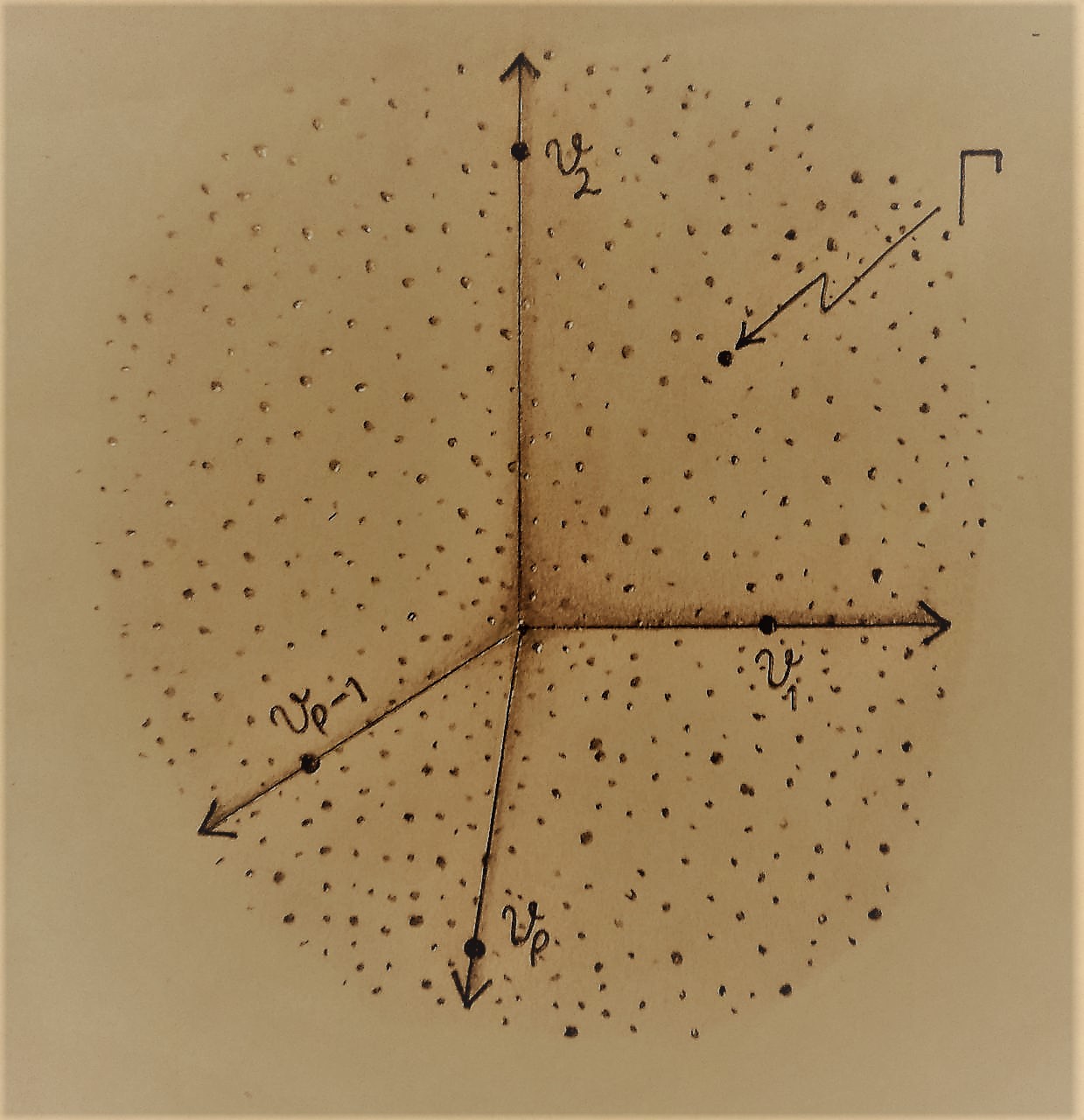
Figure 2. A quantum fan (Δ,v)(\Delta,v) in Γ\Gamma is very similar to a classical fan Δ\Delta in toric geometry, but instead of an integral lattice, it is equipped with a q-lattice Γ\Gamma (cf. Definition 4.1). Notice that we must mark the (non-canonical) ‘primitive vectors’ (v1,…,vp)(v_{1},\ldots,v_{p}) (all in Γ\Gamma) on every ray of the 11-skeleton of the fan. The fan Δ\Delta no longer needs to be rational.

A general quantum toric stack can be constructed starting from a general (not necessarily rational) quantum fan (see Figure 2 and Definition 4.1): such a q-fan carried a q-lattice Γ⊂ℝd\Gamma\subset{\mathbb{R}}^{d}, and therefore defines a q-torus 𝒯ℂ,d,Γ≅[ℂd/Γ]{\mathscr{T}}_{{\mathbb{C}},d,\Gamma}\cong[{\mathbb{C}}^{d}/\Gamma]. The quantum toric stack 𝒳Δ,Γ,v{\mathscr{X}}_{\Delta,\Gamma,v} (cf. Definition 5.8) is an equivariant compactification of 𝒯ℂ,d,Γ{\mathscr{T}}_{{\mathbb{C}},d,\Gamma} given by the data of the quantum fan (Δ,v)(\Delta,v).

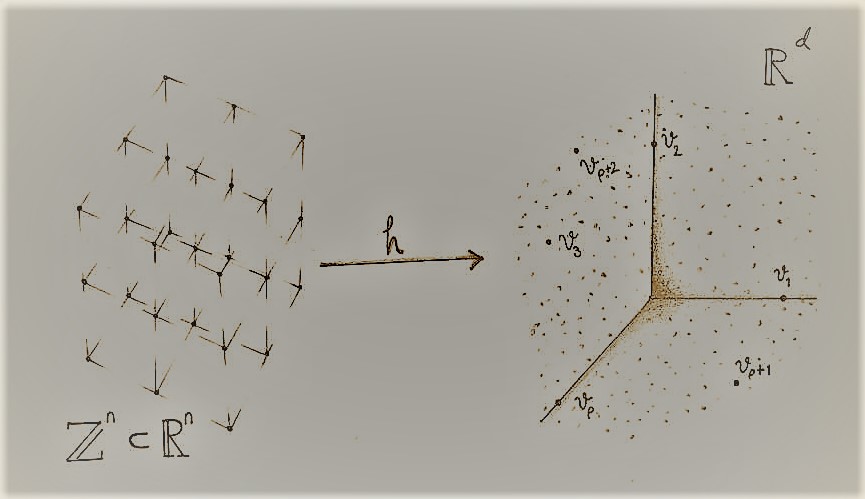
As explained before, we really want to consider the calibrated case (adding gerbe degrees of freedom). At the level of fans, this is achieved by the definition of a calibrated quantum fan. The precise description of a calibrated quantum fan (depicted in Figure 3) is found in Definition 4.9 below. For now, think of a calibration as a homomorphism h:ℤn→Γh:{\mathbb{Z}}^{n}\to\Gamma. Given such a calibrated quantum fan, then we define a Calibrated Quantum Toric Stack in Definition 6.17 and denoted88 8 Here JJ is a certain crucial piece of combinatorial data the we are omitting altogether in the introduction but see Definition 4.9 for details. by 𝒳Δ,h,Jc​a​l{\mathscr{X}^{cal}_{\Delta,h,J}}.

Refer to caption
Figure 3. A calibrated quantum fan (Δ,h)(\Delta,h) is essentially a quantum fan plus a calibration, namely, a homomorphism h:ℤn→Γh:{\mathbb{Z}}^{n}\to\Gamma ‘determining the various Planck lengths of the quantum system’ (cf. Definition 4.9).

The relation between the calibrated Quantum Toric stack 𝒳Δ,h,Jc​a​l{\mathscr{X}^{cal}_{\Delta,h,J}} and its un-calibrated version 𝒳Δ,Γ,v{\mathscr{X}_{\Delta,\Gamma,v}} is explained in Proposition 6.20; 𝒳Δ,h,Jc​a​l{\mathscr{X}^{cal}_{\Delta,h,J}} is a gerbe over 𝒳Δ,Γ,v{\mathscr{X}_{\Delta,\Gamma,v}} with band ℤa{\mathbb{Z}}^{a} (where a:=n−rankℤ​(Γ)a:=n-\mathrm{rank}_{\mathbb{Z}}(\Gamma)): 𝒳Δ,h,Jc​a​l{\mathscr{X}^{cal}_{\Delta,h,J}} is completely determined by a classifying map 𝒳Δ,Γ,v→ℬ​ℬ​ℤ{\mathscr{X}_{\Delta,\Gamma,v}}\to{\mathscr{B}}{\mathscr{B}}{\mathbb{Z}}.

One of the main results of this paper is Theorem 6.24: the category of simplicial calibrated Quantum Toric Stacks 𝒬c​a​l\mathscr{Q}^{cal} is equivalent to the category of quantum toric fans Qc​a​lQ^{cal}.

The Quantum Geometric Invariant Theory (QGIT) corresponding to quantum toric geometry is specially interesting: we prove that one can indeed represent 𝒳Δ,h,Jc​a​l{\mathscr{X}^{cal}_{\Delta,h,J}} as a global quotient of the form (cf. Theorem 7.6):

𝒳Δ,h,Jc​a​l≅[𝒮/𝒜],{\mathscr{X}^{cal}_{\Delta,h,J}}\cong[\mathscr{S}/\mathcal{A}],

where 𝒮\mathscr{S} is the complement in ℂn{\mathbb{C}}^{n} of a union of coordinate vector subspaces and the classical torus 𝕋n{\mathbb{T}}^{n} acts multiplicatively on it with a Zariski dense orbit (we denote by 𝒜\mathcal{A} this action). Moreover, 𝒜\mathcal{A} actually defines a foliation on 𝒮\mathscr{S} so that the stackification of the holonomy groupoid of said foliation is isomorphic to the un-calibrated toric stack 𝒳Δ,Γ,v{\mathscr{X}_{\Delta,\Gamma,v}} (Theorem 7.10).

From the point of view of QGIT, there is a deep and beautiful relation beetween quantum toric stacks and LVMB theory (see section 8 for definitions). Such relation occurs only when n−dn-d is even (cf. Definition 9.2). The reader may want to think for now of a LVMB-manifold (together with a canonical foliation induced by a holomorphic CmC^{m}-action) (N,ℱ)(N,{\mathcal{F}}) as a generalization of the Calabi-Eckmann manifolds (and their elliptic foliation induced by a ℂ{\mathbb{C}}-action, where ℂ{\mathbb{C}} covers the elliptic curve) so that (cf. Theorem 9.13):

𝒳Δ,Γ,v≅[N/ℱ]{\mathscr{X}_{\Delta,\Gamma,v}}\cong[N/{\mathcal{F}}]

and

𝒳Δ,h,Jc​a​l≅[N/ℂm].{\mathscr{X}^{cal}_{\Delta,h,J}}\cong[N/{\mathbb{C}}^{m}].

Furthermore, we will show (Theorem 9.19) that the category 𝒱L​V​M​B∗\mathscr{V}^{*}_{LVMB} of LVMB-manifolds is equivalent to the full subcategory 𝒬e​v​e​nc​a​l\mathscr{Q}^{cal}_{even} of 𝒬c​a​l\mathscr{Q}^{cal} whose objects are calibrated Quantum Toric Stacks associated to an even calibrated Quantum Fan. To deal with the odd case, we could consider Ishida’s theory [32]. There, Ishida considers compact complex manifolds MM with maximal real-torus action. Complete toric varieties and LVMB manifolds are examples of such manifolds. Just like LVMB-manifolds, these manifolds are also endowed with a canonical holomorphic foliation and the leaf stacks of such foliations are always Quantum toric stacks, landing sometimes in the case when n−dn-d is odd (cf. Remark 9.16). In any case, this method provides a way to interpret QGIT for the odd case. By using Ishida’s results [30], we can also prove that 𝒳Δ,Γ,v{\mathscr{X}_{\Delta,\Gamma,v}} is Kähler iff Δ\Delta is polytopal, for an appropriate definition of Kähler in this context (Theorem 10.2). In the polytopal case that has been just considered, the image of the quantum moment map is described in Subsection 8.4, and the inverse image of a point in the polytope is a real lagrangian quantum torus.
Refer to caption
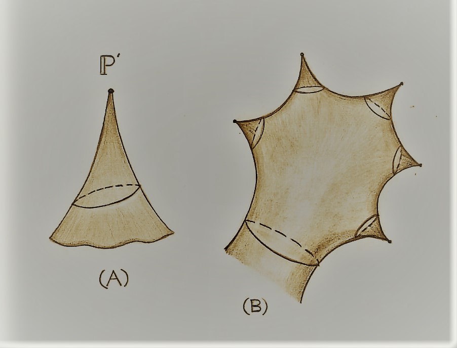
Figure 4. Moduli spaces of quantum toric stacks: in (A) we depict the moduli space of quantum projective lines: it has only one orbifold point with stabilizer ℤ2{\mathbb{Z}}_{2} corresponding to the classical ℙ1{\mathbb{P}}^{1} (or equivalently, to its non-commutative avatar ℂ​𝒫01{\mathbb{C}}{\mathscr{P}}^{1}_{0}); for the case of ℙd{\mathbb{P}}^{d}, see Subsection 11.4. In (B) we depict a more fanciful representation of the moduli space ℳ^toricD,n,d{\hat{\mathscr{M}}_{\mathrm{toric}}^{D,n,d}} of calibrated Quantum Toric Stacks with fixed combinatorial type DD: the orbifold points occur whenever the fan suddenly has more symmetries (cf. Section 11). The classical toric varieties will land on the rational locus of some of these moduli spaces.

Unlike classical toric varieties which are rigid (as equivariant toric spaces), quantum toric stacks admit moduli. In Section 11, the final section of this paper, we study various moduli spaces, specially the moduli space ℳtoricD,d{\mathscr{M}_{\mathrm{toric}}^{D,d}} of quantum toric stacks with fixed combinatorial type DD (and Γ\Gamma-complete), the moduli space ℳ^toricD,n,d{\hat{\mathscr{M}}_{\mathrm{toric}}^{D,n,d}} of calibrated Quantum Toric Stacks (of maximal length) and fixed combinatorial type DD and the moduli space ℳm,n𝒮\mathcal{M}^{\mathcal{S}}_{m,n} of GG-biholomorphism classes of LVMB manifolds (see Figure 4). The main theorem of this final section is that that all those moduli spaces are real finite-dimensional orbifolds (cf. Corollary 11.13, Corollary 11.18 and Proposition 11.27). Under certain numerical condition (that of Theorem 11.28), more is true: ℳm,n𝒮\mathcal{M}^{\mathcal{S}}_{m,n} is a complex orbifold, and there is a ‘twistor bundle complexification mapping’:

ℝ(n−d)2/2→ℳm,n𝒮→ℳ^toricD,n,d,{\mathbb{R}}^{(n-d)^{2}/2}\to{\mathcal{M}^{\mathcal{S}}_{m,n}}\to{\hat{\mathscr{M}}_{\mathrm{toric}}^{D,n,d}},

namely, ℳm,n𝒮{\mathcal{M}^{\mathcal{S}}_{m,n}} is a (sometimes complex) orbibundle of even rank (n−d)2/2(n-d)^{2}/2 over ℳ^toricD,n,d{\hat{\mathscr{M}}_{\mathrm{toric}}^{D,n,d}}. This immediately implies the homotopy equivalence (a diffeomorphism when n=dn=d):

ℳm,n𝒮≃ℳ^toricD,n,d,{\mathcal{M}^{\mathcal{S}}_{m,n}}\simeq{\hat{\mathscr{M}}_{\mathrm{toric}}^{D,n,d}},

namely, the moduli space ℳ^toricD,n,d{\hat{\mathscr{M}}_{\mathrm{toric}}^{D,n,d}} can be promoted (in the same homotopy class) to a complex orbifold ℳm,n𝒮{\mathcal{M}^{\mathcal{S}}_{m,n}}. Let us point out here that there is an interesting analogy with the classical case of the moduli space of curves M⁡(g,n)M(g,n) where gg is the genus (combinatorial information) and nn is a marking that makes the compactification of the moduli space nicer. Here too, we have combinatorial information (D,d)(D,d), and marking information nn, making the moduli space nicer, and even sometimes giving it a complex structure. We will explore this analogy elsewhere.

Let us finish this introduction by adding some very schematic and cursory remarks regarding future work on the relation of this theory to the field of mirror symmetry. It is natural to ask for a generalization of Homological Mirror Symmetry for toric varieties. Classical HMS for ordinary toric varieties has been proved by Abouzaid [1] using methods from tropical geometry. It can be considered as a SYZ (Strominger-Yau-Zaslow) correspondence based on family of Lagrangian tori over a polytope. The methods of this paper can be used to obtain a quantization of the corresponding Lagrangian tori and of the fan associated to the polytope. It is reasonable to expect that HMS generalizes to this situation. This could be understood as a quantum version of the SYZ-correspondance. All the non-commutative projective spaces of the work of Auroux, Katzarkov and Orlov[3] on mirror symmetry projective spaces, appear as quantum toric stacks, and that we expect many of the results of [3] to generalize to our setting. There is a specially simple and interesting example of an LVM manifold: the classical Hopf surface S3×S1S^{3}\times S^{1}. As we have discussed earlier, it has a canonical elliptic foliation that, when deformed, covers all quantum toric projective lines. Using TT-duality for quantum tori, we can understand ‘mirror symmetry’ for the Hopf surface giving an alternative approach to the one developed by Abigail Ward in her Harvard PhD thesis. From this point of view it is also natural to characterize the moduli space of stability conditions for non-commutative toric varieties considered as triangulated categories (cf. [54, 4, 38, 39, 33]): we conjecture that they are closely related to the solenoidal spaces as studied by Sullivan-Verjovsky [55].

The previous program seems to beg a solution to the question as to the correct formulation of an algebraic geometry (the so called BB-side) that allows one to define the adequate categories associated to a quantum toric stack. Two puzzles must be met: first, the stacks constructed in this paper are far from being algebraic, and second, even in the Kähler case, they are constructed starting from non-symplectic manifolds such as the Hopf surface. All the difficulties can be resolved simultaneously by the introduction of a version of algebraic geometry that occurs in a fixed non-standard extension of the complex numbers. We have investigated and introduced such ‘chimeric algebraic geometry’ in a series of works [40, 34] (cf. [26], [27],[37]). Then, the theory offered in [34] solves the issue of constructing the desired BB-side for the mirror symmetry program, on the other hand, the symplectic geometry needed for the AA-side remains an outstading question requiring further analysis. We will return to this issue elsewhere.

Finally, the theory we present here is, as we said before, a wide ranging generalization of toric geometry. There were earlier approaches generalizaing toric geometry in a number of ways, and they are in various ways related to our theory. Let us simply refer the reader to some of the most relevant works in this direction: Battaglia-Prato [5], Battaglia-Zaffran [6], Bressler-Lunts [13], Firat Pir [24], Ford [25], Postinghel-Sottile [48], and Ratiu-Zung [51].

Acknowledgments. L.K. was supported by the Simons collaborative Grant - HMS, NRU HSE, RF government grant, ag. 14.641.31.000, Simons Principle Investigator Grant, CKGA VIHREN grant KΠ\Pi-06-Π\PiB/16. Much of the research was conducted while the authors enjoyed the hospitality of IMSA Miami and Laboratory of Mirror Symmetry HSE Moscow.

E.L. would like to thank FORDECYT (CONACYT), IMATE-UNAM, NRU HSE, RF government grant, ag. 14.641.31.000, the Institute for Mathematical Sciences of the Americas, the Simon’s Foundation and the Moshinsky Foundation, the University of Geneva, the QUANTUM project from the University of Angers and the Laboratory of Mirror Symmetry HSE Moscow.

L.M. would like to thank the kind support of the QUANTUM project from the University of Angers, UMI CNRS 2001 LaSol and the Institute for Mathematical Sciences of the Americas (Simons Foundation and University of Miami).

A.V. would like to thank the support of the University of Angers, QUANTUM project UMI CNRS 2001 LaSo, IMSA in Miami and DGAPA PAPIIT project IN108120 UNAM, Mexico.

2. Conventions on Stacks

In this section, we fix some notations and conventions on the stacks that will be used in the paper. These include all the Quantum Toric Stacks and all calibrated Quantum Toric Stacks; however, the orbifolds of Section 11 are not instances of what follows; they are briefly defined in Remark 11.14.

Remark 2.1.

This section can be skipped by readers that are not familiar with the theory of stacks. Such a reader can think of a stack as a ‘manifold whose charts are not one-to-one’ very similar to orbifolds. All our stacks will have local charts of the form V→V/𝐆V\to V/\mathbf{G} where the local group 𝐆\mathbf{G} is discrete and abelian (not quite finite, as in the case of orbifolds). Nevertheless a warning is in order: for most quantum toric varieties, the quotient of a local chart V/𝐆V/\mathbf{G} will not be Hausdorff much like in the theory of quasifolds [50]; still, we use the theory of stacks for we need the whole machinery of morphisms of stacks, fibered products, etc. in our development. Surprisingly, we could have used all the required machinery using the theory of diffeological spaces [29] to model our quantum toric manifolds as it is shown on [8] (but the morphisms would still be a bit off). In any case, we prefer the more standard use of stacks presented here.

We take as base category the category 𝔄\mathfrak{A} of affine toric varieties and toric morphisms. We take for covering of an affine toric variety TT a decomposition T=T1∪⋯∪TnT=T_{1}\cup\cdots\cup T_{n} into toric Zariski open subsets of TT. With these coverings, 𝔄\mathfrak{A} is a site.

We will also need the category 𝔊\mathfrak{G} of complex analytic spaces XX endowed with a holomorphic action of a complex abelian Lie group GG with a Zariski open orbit isomorphic to GG. Morphisms are equivariant holomorphic mappings that restrict to Lie group morphisms. Observe that 𝔄\mathfrak{A} is a subcategory of 𝔊\mathfrak{G}.

By a cover of TT of 𝔄\mathfrak{A}, we mean an object T~\tilde{T} of 𝔊\mathfrak{G} endowed with a free and proper holomorphic action of a discrete abelian group HH whose quotient is TT. Hence p:T~→Tp:\tilde{T}\to T is an unramified analytic cover of TT. Moreover, pp is equivariant, that is, belongs to 𝔊\mathfrak{G} since the abelian HH-action commutes with the abelian GG-action.

If HH is a non-discrete complex abelian Lie group acting freely and properly on T~\tilde{T} with quotient TT, then p:T~→Tp:\tilde{T}\to T is an equivariant principal HH-bundle and we rather speak of a principal bundle over TT.

Quantum Toric Stacks are of the form [X/H][X/H] with X∈𝔊X\in\mathfrak{G} and HH a discrete abelian group or a complex abelian Lie group, or are descent data of such [X/H][X/H], cf. Section 5. To be more precise, we consider the category [X/H][X/H] whose objects are covers T~\tilde{T} over a space T∈𝔄T\in\mathfrak{A} with an equivariant holomorphic map mm

(2.1) T~{\lx@inpgf@ignorespaces\tilde{T}}X{\lx@inpgf@ignorespaces X}T{\lx@inpgf@ignorespaces T}m\scriptstyle{\lx@inpgf@ignorespaces m}

Here mm is assumed to be equivariant with respect to both the HH-action and the GG-action.

The morphisms are

(2.2) X{\lx@inpgf@ignorespaces X}T~{\lx@inpgf@ignorespaces\tilde{T}}S~{\lx@inpgf@ignorespaces\tilde{S}}T{\lx@inpgf@ignorespaces T}S{\lx@inpgf@ignorespaces S}m\scriptstyle{\lx@inpgf@ignorespaces m}n\scriptstyle{\lx@inpgf@ignorespaces n}

The following proposition is enough for our purposes.

Proposition 2.2.

The functor [X/H]→𝔄[X/H]\to\mathfrak{A} sending (T~,T,m)(\tilde{T},T,m) onto TT; and (T~→S~,T→S,m,n)(\tilde{T}\to\tilde{S},T\to S,m,n) onto T→ST\to S is a stack over 𝔄\mathfrak{A}.

Proof.

We must check that pull-backs exist and are unique up to unique isomorphism, that isomorphisms form a sheaf and that descent data are effective.

Given a cartesian diagram

(2.3) Tf×pS~{\lx@inpgf@ignorespaces T_{f}\times_{p}\tilde{S}}S~{\lx@inpgf@ignorespaces\tilde{S}}T{\lx@inpgf@ignorespaces T}S{\lx@inpgf@ignorespaces S}p\scriptstyle{\lx@inpgf@ignorespaces p}f\scriptstyle{\lx@inpgf@ignorespaces f}

its restriction to the Zariski open orbits is

(2.4) (ℂ∗)fa×pG{\lx@inpgf@ignorespaces({\mathbb{C}}^{*})^{a}_{f}\times_{p}G}G{\lx@inpgf@ignorespaces G}(ℂ∗)a{\lx@inpgf@ignorespaces({\mathbb{C}}^{*})^{a}}(ℂ∗)b{\lx@inpgf@ignorespaces({\mathbb{C}}^{*})^{b}}p\scriptstyle{\lx@inpgf@ignorespaces p}f\scriptstyle{\lx@inpgf@ignorespaces f}

with aa, respectively bb, the dimension of TT, resp. S. Now, (ℂ∗)fa×pG({\mathbb{C}}^{*})^{a}_{f}\times_{p}G is a complex Lie abelian group, with the following law

(2.5) (w,g)⋅(w′,g′)=(w⋅w′,g⋅g′)(w,g)\cdot(w^{\prime},g^{\prime})=(w\cdot w^{\prime},g\cdot g^{\prime})

which is well defined since f⁡(w⋅w′)=f⁡(w)⋅f⁡(w′)=p⁡(g)⋅p⁡(g′)=p⁡(g⋅g′)f(w\cdot w^{\prime})=f(w)\cdot f(w^{\prime})=p(g)\cdot p(g^{\prime})=p(g\cdot g^{\prime}).

But (2.5) extends as an equivariant holomorphic action of (ℂ∗)fa×pG({\mathbb{C}}^{*})^{a}_{f}\times_{p}G on Tf×pS~T_{f}\times_{p}\tilde{S}. It has obviously a Zariski open orbit isomorphic to (ℂ∗)fa×pG({\mathbb{C}}^{*})^{a}_{f}\times_{p}G and all the arrows of (2.3) are equivariant. Thus pull-back exist and it is straightforward to check that they are unique up to unique isomorphisms of 𝔊\mathfrak{G}.

The last two points (isomorphisms form a sheaf and descent data are effective) are routine checking and we leave their verification to the reader. ∎

The choice of 𝔄\mathfrak{A} as base category reflects the fact that we consider Quantum Toric Stacks as a generalization of classical toric varieties. The choice of equivariant covers reflects the fact that we only deal with equivariant properties of these geometric objects. Of course, other choices - as taking 𝔊\mathfrak{G} or taking the category of analytic spaces as base category, using equivariant covers or not - may have their interest and should be developed to look for different flavours of the construction.

We finish this section with a warning.

Warning 2.3.

Quantum Toric Stacks are not algebraic stacks. Many of them have stabilizers equal to some power of ℤ{\mathbb{Z}}. And even when it is not the case, the intensive and fundamental role played by the exponential map EE defined in (3.11) prevents them from being algebraic.

However, since Quantum Toric Stacks have an atlas which is an analytic space, cf. Corollaries 7.11 and 7.9, they are analytic in the sense of [43, §2.4].

3. Quantum Tori

In this section, we define the Quantum Tori which sit inside Quantum Toric Varieties. They are complex analogues of 𝒯ℝ,ℏi{\mathscr{T}}_{{\mathbb{R}},\hbar}^{i} but the precise relationship is not investigated here but in Section 11, see Theorem 11.4.

3.1. Quantum Torus associated to an additive subgroup of ℝd{\mathbb{R}}^{d}

In classical toric geometry, there is a single complex torus 𝕋d:=𝕋ℂd{\mathbb{T}}^{d}:={\mathbb{T}}^{d}_{\mathbb{C}} once the dimension dd is fixed. In a more intrinsic presentation, for any lattice Γ\Gamma that spans ℝd{\mathbb{R}}^{d} over the reals, is associated a torus Hom ​(Γˇ,ℂ∗)\text{Hom }(\check{\Gamma},{\mathbb{C}}^{*}), but all are isomorphic to 𝕋d{\mathbb{T}}^{d}.

In Quantum Toric Geometry, things are different since Γ\Gamma is no more a lattice but any finitely generated additive subgroup of some ℝd{\mathbb{R}}^{d} spanning it over the reals (a q-lattice). Then we define,

Definition 3.1.

The quantum torus associated to Γ\Gamma is the quotient stack [ℂd/Γ][{\mathbb{C}}^{d}/\Gamma]. We denote it by 𝒯d,Γ{\mathscr{T}_{d,\Gamma}}.

Example 3.2.

Let d=1d=1 and define Γ\Gamma as the subgroup of (ℝ,+)({\mathbb{R}},+) generated by 11 and 2\sqrt{2}. Since 2\sqrt{2} is irrational, it is dense in ℝ{\mathbb{R}}. It acts freely on ℝ{\mathbb{R}} by translation but this action is not proper and the topological quotient is not Hausdorff. Indeed, for any pair of real numbers x,yx,y, since y−xy-x is an accumulation point of Γ\Gamma, the images of xx and yy are not separated.
It follows that the associated quantum torus [ℂ/Γ][{\mathbb{C}}/\Gamma] is not a manifold and stack language is needed to handle it as a complex ”space”.

Hence 𝒯d,Γ=[ℂd/Γ]{\mathscr{T}_{d,\Gamma}}=[{\mathbb{C}}^{d}/\Gamma] has to be understood more formally as a category fibered in groupoids 𝒯d,Γ→𝔄{\mathscr{T}_{d,\Gamma}}\to\mathfrak{A}, as in Section 2.

Objects of 𝒯d,Γ{\mathscr{T}_{d,\Gamma}} are Γ\Gamma-covers TT over a space A∈𝔄A\in\mathfrak{A} with an equivariant holomorphic map mm in ℂd{\mathbb{C}}^{d}

(3.1) T{\lx@inpgf@ignorespaces T}ℂd{\lx@inpgf@ignorespaces{\mathbb{C}}^{d}}A{\lx@inpgf@ignorespaces A}m\scriptstyle{\lx@inpgf@ignorespaces m}

and morphisms

(3.2) ℂd{\lx@inpgf@ignorespaces{\mathbb{C}}^{d}}T{\lx@inpgf@ignorespaces T}S{\lx@inpgf@ignorespaces S}A{\lx@inpgf@ignorespaces A}B{\lx@inpgf@ignorespaces B}m\scriptstyle{\lx@inpgf@ignorespaces m}n\scriptstyle{\lx@inpgf@ignorespaces n}

The functor 𝒯d,Γ→𝔄{\mathscr{T}_{d,\Gamma}}\to\mathfrak{A} sends (T,A,m)(T,A,m) onto AA; and (T→S,A→B,m,n)(T\to S,A\to B,m,n) onto A→BA\to B.

If LL is a linear map from ℝd{\mathbb{R}}^{d} to ℝd′{\mathbb{R}}^{d^{\prime}} that sends Γ\Gamma onto Γ′\Gamma^{\prime}, then its extension over the complex numbers obviously descends as a stack morphism from 𝒯d,Γ{\mathscr{T}_{d,\Gamma}} onto 𝒯d′,Γ′{\mathscr{T}_{d^{\prime},\Gamma^{\prime}}}.

(3.3) ℝd{\lx@inpgf@ignorespaces{\mathbb{R}}^{d}}ℝd′{\lx@inpgf@ignorespaces{\mathbb{R}}^{d^{\prime}}}ℂd{\lx@inpgf@ignorespaces{\mathbb{C}}^{d}}ℂd′{\lx@inpgf@ignorespaces{\mathbb{C}}^{d^{\prime}}}𝒯d,Γ{\lx@inpgf@ignorespaces{\mathscr{T}_{d,\Gamma}}}𝒯d′,Γ′{\lx@inpgf@ignorespaces{\mathscr{T}_{d^{\prime},\Gamma^{\prime}}}}L\scriptstyle{\lx@inpgf@ignorespaces L}L\scriptstyle{\lx@inpgf@ignorespaces L}ℒ\scriptstyle{\lx@inpgf@ignorespaces\mathscr{L}}

We take this as definition of toric morphism. Hence,

Definition 3.3.

A torus morphism ℒ\mathscr{L} from 𝒯d,Γ{\mathscr{T}_{d,\Gamma}} onto 𝒯d′,Γ′{\mathscr{T}_{d^{\prime},\Gamma^{\prime}}} is a stack morphism such that there exists a linear map LL from ℝd{\mathbb{R}}^{d} to ℝd′{\mathbb{R}}^{d^{\prime}} sending Γ\Gamma to Γ′\Gamma^{\prime} and satisfying (3.3).

To wit, given T→AT\to A a Γ\Gamma-cover, set

(3.4) T×LΓ′:={(t,γ′)∈T×Γ′}/ΓT\times_{L}\Gamma^{\prime}:=\{(t,\gamma^{\prime})\in T\times\Gamma^{\prime}\}/\Gamma

for the following action of Γ\Gamma

(3.5) γ⋅(t,γ′)=(γ⋅t,γ′−L​γ)\gamma\cdot(t,\gamma^{\prime})=(\gamma\cdot t,\gamma^{\prime}-L\gamma)

Let also

(3.6) [(t,γ′)]⟼m′​[(t,γ′)]:=L​m​(t)+γ′[(t,\gamma^{\prime})]\longmapsto m^{\prime}[(t,\gamma^{\prime})]:=Lm(t)+\gamma^{\prime}

which is well-defined since

L​m​(γ⋅t,γ′−L​γ)\displaystyle Lm(\gamma\cdot t,\gamma^{\prime}-L\gamma) =L​m​(γ⋅t)+γ′−L​γ\displaystyle=Lm(\gamma\cdot t)+\gamma^{\prime}-L\gamma
=L​m​(t)+L​γ+γ′−L​γ\displaystyle=Lm(t)+L\gamma+\gamma^{\prime}-L\gamma
=L​m​(t)+γ′\displaystyle=Lm(t)+\gamma^{\prime}

Given f:T→Sf:T\to S a morphism of Γ\Gamma-cover, over A→BA\to B, we define

(3.7) [(t,γ′)]∈T×LΓ′⟼fL​([(t,γ′)]:=[(f⁡(t),γ′)])∈S×LΓ′[(t,\gamma^{\prime})]\in T\times_{L}\Gamma^{\prime}\longmapsto f_{L}([(t,\gamma^{\prime})]:=[(f(t),\gamma^{\prime})])\in S\times_{L}\Gamma^{\prime}

and, if mm, resp. nn, is the equivariant map associated to T→AT\to A, resp. S→BS\to B, so that m=n∘fm=n\circ f, we have

n′∘fL​([(t,γ′)])\displaystyle n^{\prime}\circ f_{L}([(t,\gamma^{\prime})]) =n′​([f⁡(t),γ′])\displaystyle=n^{\prime}([f(t),\gamma^{\prime}])
=L​n​(f⁡(t))+γ′\displaystyle=Ln(f(t))+\gamma^{\prime}
=L​m​(t)+γ′\displaystyle=Lm(t)+\gamma^{\prime}
=m′​([t,γ′])\displaystyle=m^{\prime}([t,\gamma^{\prime}])

So we finally have

(3.8) ℒ⁡(T,A,m)=(T×LΓ′,A,m′)\mathscr{L}(T,A,m)=(T\times_{L}\Gamma^{\prime},A,m^{\prime})

and

(3.9) ℒ\displaystyle\mathscr{L} (f:T→S,A→B,m,n)=(fL:T×LΓ′→S×LΓ′,\displaystyle(f:T\to S,A\to B,m,n)=(f_{L}:T\times_{L}\Gamma^{\prime}\to S\times_{L}\Gamma^{\prime},
A→B,m′,n′)\displaystyle A\to B,m^{\prime},n^{\prime})

Since Vect ​Γ\text{Vect }\Gamma is the whole ℂd{\mathbb{C}}^{d}, there exists a basis of ℂd{\mathbb{C}}^{d} formed by vectors (v1,…,vd)(v_{1},\ldots,v_{d}) of Γ\Gamma. We may assume that is such a basis. There exists some linear isomorphism LL of ℂd{\mathbb{C}}^{d} sending (v1,…,vd)(v_{1},\ldots,v_{d}) onto the canonical basis (e1,…,ed)(e_{1},\ldots,e_{d}). It defines a torus isomorphism between 𝒯d,Γ{\mathscr{T}_{d,\Gamma}} and 𝒯d,L​Γ{\mathscr{T}_{d,L\Gamma}}.

So, defining

Definition 3.4.

Let (e1,…,ed)(e_{1},\ldots,e_{d}) be the canonical basis of ℝd{\mathbb{R}}^{d}. We say that Γ\Gamma is standard if it contains the standard lattice ⨁i=1dℤ​ei\bigoplus_{i=1}^{d}{\mathbb{Z}}e_{i}.
We say that 𝒯d,Γ{\mathscr{T}_{d,\Gamma}} is standard if Γ\Gamma is standard.

We just proved

Lemma 3.5.

Any quantum torus is isomorphic to a standard quantum torus.

If Γ\Gamma is standard, we may decompose it as

(3.10) Γ=ℤd+Γ0\Gamma={\mathbb{Z}}^{d}+\Gamma_{0}

Define

(3.11) x∈ℝd⊂ℂd⟼E⁡(x):=(e2​i​π​x1,…,e2​i​π​xd)∈(𝕊1)d⊂𝕋dx\in{\mathbb{R}}^{d}\subset{\mathbb{C}}^{d}\longmapsto E(x):=(e^{2i\pi x_{1}},\ldots,e^{2i\pi x_{d}})\in(\mathbb{S}^{1})^{d}\subset{\mathbb{T}}^{d}

Then we may put a standard 𝒯d,Γ{\mathscr{T}_{d,\Gamma}} in multiplicative form as the quotient stack [𝕋d/E⁡(Γ)][{\mathbb{T}}^{d}/E(\Gamma)] where E⁡(Γ)=E⁡(Γ0)E(\Gamma)=E(\Gamma_{0}) acts multiplicatively on 𝕋d{\mathbb{T}}^{d}. We have a commutative diagram

(3.12) ℂd{\lx@inpgf@ignorespaces{\mathbb{C}}^{d}}𝕋d{\lx@inpgf@ignorespaces{\mathbb{T}}^{d}}𝒯d,Γ{\lx@inpgf@ignorespaces{\mathscr{T}_{d,\Gamma}}}[𝕋d/E⁡(Γ)]{\lx@inpgf@ignorespaces\phantom{d}\kern-5.0pt[{\mathbb{T}}^{d}/E(\Gamma)]}E\scriptstyle{\lx@inpgf@ignorespaces E}≃\scriptstyle{\lx@inpgf@ignorespaces\simeq}

In a more functorial point of view, EE defines a stack isomorphism ℰ\mathscr{E} from 𝒯d,Γ{\mathscr{T}_{d,\Gamma}} to [𝕋d/E⁡(Γ0)][{\mathbb{T}}^{d}/E(\Gamma_{0})] such that

ℰ⁡(T,A,m)=(T/ℤd,A,E​m)\mathscr{E}(T,A,m)=(T/{\mathbb{Z}}^{d},A,Em)

with ℤd{\mathbb{Z}}^{d} acts on TT as a subgroup of Γ\Gamma and with

T{\lx@inpgf@ignorespaces T}ℂd{\lx@inpgf@ignorespaces{\mathbb{C}}^{d}}T/ℤd{\lx@inpgf@ignorespaces T/{\mathbb{Z}}^{d}}𝕋d{\lx@inpgf@ignorespaces{\mathbb{T}}^{d}}A{\lx@inpgf@ignorespaces A}m\scriptstyle{\lx@inpgf@ignorespaces m}E\scriptstyle{\lx@inpgf@ignorespaces E}E​m\scriptstyle{\lx@inpgf@ignorespaces Em}

and

ℰ(f:T→S,A→B,m,n)=(f:T/ℤd→S/ℤd,A→B,Em,En)\mathscr{E}(f:T\to S,A\to B,m,n)=(f:T/{\mathbb{Z}}^{d}\to S/{\mathbb{Z}}^{d},A\to B,Em,En)

where ff descends as a morphism from T/ℤdT/{\mathbb{Z}}^{d} to S/ℤdS/{\mathbb{Z}}^{d} since it satisfies by definition f⁡(p⋅t)=p⋅f⁡(t)f(p\cdot t)=p\cdot f(t) for all p∈Γp\in\Gamma.

Example 3.6.

Let d=1d=1 and Γ\Gamma be generated by 11 and 2\sqrt{2} as in Example 3.2. Consider the linear map

z∈ℂ⟼2⋅z∈ℂz\in{\mathbb{C}}\longmapsto\sqrt{2}\cdot z\in{\mathbb{C}}

It sends 11 onto 2\sqrt{2} and 2\sqrt{2} onto 22 hence it preserves Γ\Gamma. So it descends as the torus morphism

[z]∈[ℂ/Γ]⟼[2​z]∈[ℂ/Γ][z]\in[{\mathbb{C}}/\Gamma]\longmapsto[\sqrt{2}z]\in[{\mathbb{C}}/\Gamma]

or, in multiplicative form,

(3.13) [w]∈[𝕋/E⁡(Γ)]⟼[w2]∈[𝕋/E⁡(Γ)][w]\in[{\mathbb{T}}/E(\Gamma)]\longmapsto[w^{\sqrt{2}}]\in[{\mathbb{T}}/E(\Gamma)]

This must be understood as follows. Given w∈𝕋w\in{\mathbb{T}}, choose z∈ℂz\in{\mathbb{C}} with E⁡(z)=wE(z)=w. Then compute E⁡(z​2)E(z\sqrt{2}). Of course, zz is unique only up to addition of an integer, and for p∈ℤ∗p\in{\mathbb{Z}}^{*}, the complex number E⁡((z+p)​2)E((z+p)\sqrt{2}) is different from E⁡(z​2)E(z\sqrt{2}). Hence there is no well defined mapping w→w2w\to w^{\sqrt{2}}. However, E⁡(p​2)E(p\sqrt{2}) belongs to E⁡(Γ)E(\Gamma) so (3.13) is well defined.

Remark 3.7.

It is important to notice that a torus morphism ℒ\mathscr{L} does not always lift as a mapping from 𝕋d{\mathbb{T}}^{d} to 𝕋d′{\mathbb{T}}^{d^{\prime}}, as shown in Example 3.6. This will be a source of problem when defining toric morphisms in Section 5.

3.2. Calibrated Quantum Tori

We define now calibrated quantum tori. To do this, we need to fix, in addition to Γ\Gamma, a set of generators of Γ\Gamma. More precisely, we set

Definition 3.8.

A calibration of Γ\Gamma is given by

  1. i)

    An epimorphism h:ℤn→Γh:{\mathbb{Z}}^{n}\to\Gamma

  2. ii)

    A subset J⊂{1,…,n}J\subset\{1,\ldots,n\} such that

    (3.14) Vect​{h⁡(ei)∣i∉J}=ℂd\text{Vect}\{h(e_{i})\mid i\not\in J\}={\mathbb{C}}^{d}

The subset JJ is called the set of virtual generators. It may be empty as in the following important example.

Example 3.9.

The trivial calibration of the standard torus. Let Γ\Gamma be ℤn{\mathbb{Z}}^{n}, so that 𝒯n,Γ{\mathscr{T}_{n,\Gamma}} is just 𝕋n{\mathbb{T}}^{n}. The trivial calibration of 𝕋n{\mathbb{T}}^{n} is h=I​dh=Id. Note that it forces the set of virtual generators to be empty.

Now we set

Definition 3.10.

The calibrated quantum torus associated to h:ℤn→Γh\ :\ {\mathbb{Z}}^{n}\to\Gamma is the quotient stack [ℂd/ℤn][{\mathbb{C}}^{d}/{\mathbb{Z}}^{n}] where ℤn{\mathbb{Z}}^{n} acts through (z,p)↦z+h⁡(p)(z,p)\mapsto z+h(p). We denote it by 𝒯h,Jc​a​l{{\mathscr{T}}^{cal}_{h,J}}.

Objects of 𝒯h,Jc​a​l{{\mathscr{T}}^{cal}_{h,J}} are ℤn{\mathbb{Z}}^{n}-covers TT over a space A∈𝔄A\in\mathfrak{A} with an equivariant map mm in ℂd{\mathbb{C}}^{d}

(3.15) T{\lx@inpgf@ignorespaces T}ℂd{\lx@inpgf@ignorespaces{\mathbb{C}}^{d}}A{\lx@inpgf@ignorespaces A}mc​a​l\scriptstyle{\lx@inpgf@ignorespaces m^{cal}}

and morphisms

(3.16) ℂd{\lx@inpgf@ignorespaces{\mathbb{C}}^{d}}T{\lx@inpgf@ignorespaces T}S{\lx@inpgf@ignorespaces S}A{\lx@inpgf@ignorespaces A}B{\lx@inpgf@ignorespaces B}mc​a​l\scriptstyle{\lx@inpgf@ignorespaces m^{cal}}nc​a​l\scriptstyle{\lx@inpgf@ignorespaces n^{cal}}

The functor 𝒯h,Jc​a​l→𝔄{{\mathscr{T}}^{cal}_{h,J}}\to\mathfrak{A} sends (T,A,mc​a​l)(T,A,m^{cal}) onto AA; and (T→S,A→B,mc​a​l,nc​a​l)(T\to S,A\to B,m^{cal},n^{cal}) onto A→BA\to B.

If LL is a linear map from ℝd{\mathbb{R}}^{d} to ℝd′{\mathbb{R}}^{d^{\prime}} that sends Γ\Gamma onto Γ′\Gamma^{\prime} and induces a toric morphism, then its extension over the complex numbers does not define a stack morphism from 𝒯h,Jc​a​l{{\mathscr{T}}^{cal}_{h,J}} onto 𝒯h′,J′c​a​l{{\mathscr{T}}^{cal}_{h^{\prime},J^{\prime}}}. We need an extra morphism HH from ℤn{\mathbb{Z}}^{n} to ℤn′{\mathbb{Z}}^{n^{\prime}} such that the following diagram is commutative.

(3.17) ℤn{\lx@inpgf@ignorespaces{\mathbb{Z}}^{n}}ℤn′{\lx@inpgf@ignorespaces{\mathbb{Z}}^{n^{\prime}}}Γ{\lx@inpgf@ignorespaces\Gamma}Γ′{\lx@inpgf@ignorespaces\Gamma^{\prime}}H\scriptstyle{\lx@inpgf@ignorespaces H}h\scriptstyle{\lx@inpgf@ignorespaces h}h′\scriptstyle{\lx@inpgf@ignorespaces h^{\prime}}L\scriptstyle{\lx@inpgf@ignorespaces L}

Now the map z∈ℂd↦L​z∈ℂd′z\in{\mathbb{C}}^{d}\mapsto Lz\in{\mathbb{C}}^{d^{\prime}} satisfies

(3.18) L⁡(z+h⁡(p))=L​z+h′​(H⁡(p))L(z+h(p))=Lz+h^{\prime}(H(p))

and descends as a stack morphism ℒc​a​l\mathscr{L}^{cal} from 𝒯h,Jc​a​l{{\mathscr{T}}^{cal}_{h,J}} onto 𝒯h′,J′c​a​l{{\mathscr{T}}^{cal}_{h^{\prime},J^{\prime}}} so we have

(3.19) ℝd{\lx@inpgf@ignorespaces{\mathbb{R}}^{d}}ℝd′{\lx@inpgf@ignorespaces{\mathbb{R}}^{d^{\prime}}}ℂd{\lx@inpgf@ignorespaces{\mathbb{C}}^{d}}ℂd{\lx@inpgf@ignorespaces{\mathbb{C}}^{d}}𝒯h,Jc​a​l{\lx@inpgf@ignorespaces{{\mathscr{T}}^{cal}_{h,J}}}𝒯h′,J′c​a​l{\lx@inpgf@ignorespaces{{\mathscr{T}}^{cal}_{h^{\prime},J^{\prime}}}}L\scriptstyle{\lx@inpgf@ignorespaces L}L\scriptstyle{\lx@inpgf@ignorespaces L}ℒc​a​l\scriptstyle{\lx@inpgf@ignorespaces\mathscr{L}^{cal}}

Now, we will ask HH to preserve the virtual generators, that is, we both impose that there exists a map ss between the sets of virtual generators JJ and J′J^{\prime} such that HH satisfies

(3.20) H⁡(ei)=es⁡(i) for i∈JH(e_{i})=e_{s(i)}\qquad\text{ for }\qquad i\in J

and that HH satisfies

(3.21) H⁡(ei)∈⨁j∉J′ℤ​ej for i∉JH(e_{i})\in\bigoplus_{j\not\in J^{\prime}}{\mathbb{Z}}e_{j}\qquad\text{ for }\qquad i\not\in J

So finally, we define

Definition 3.11.

A calibrated torus morphism ℒc​a​l\mathscr{L}^{cal} from 𝒯h,Jc​a​l{{\mathscr{T}}^{cal}_{h,J}} onto 𝒯h′,J′c​a​l{{\mathscr{T}}^{cal}_{h^{\prime},J^{\prime}}} is a stack morphism such that there exists a linear map LL from ℝd{\mathbb{R}}^{d} to ℝd′{\mathbb{R}}^{d^{\prime}}, a linear map HH from ℝn{\mathbb{R}}^{n} to ℝn′{\mathbb{R}}^{n^{\prime}} and a map ss from JJ to J′J^{\prime} satisfying (3.17), (3.18), (3.19) as well as (3.20) and finally (3.21).

It is a isomorphism if the three of LL, HH and ss are isomorphisms. And it is a marked isomorphism if, moreover, JJ is equal to J′J^{\prime} and ss is the identity.

To wit, given T→AT\to A a ℤn{\mathbb{Z}}^{n}-cover, set

(3.22) T×Hℤn′:={(t,q′)∈T×ℤn′}/ℤnT\times_{H}{\mathbb{Z}}^{n^{\prime}}:=\{(t,q^{\prime})\in T\times{\mathbb{Z}}^{n^{\prime}}\}/{\mathbb{Z}}^{n}

for the following action of ℤn{\mathbb{Z}}^{n}

(3.23) p⋅(t,q′)=(p⋅t,q′−H⁡(p))p\cdot(t,q^{\prime})=(p\cdot t,q^{\prime}-H(p))

Let also

(3.24) [(t,q′)]⟼(mc​a​l)′​[(t,q′)]:=L​mc​a​l​(t)+h′​(q′)[(t,q^{\prime})]\longmapsto(m^{cal})^{\prime}[(t,q^{\prime})]:=Lm^{cal}(t)+h^{\prime}(q^{\prime})

which is well-defined since

L​mc​a​l​(p⋅t,q′−H⁡(p))\displaystyle Lm^{cal}(p\cdot t,q^{\prime}-H(p)) =L​mc​a​l​(p⋅t)+h′​(q′)−h′​H​(p)\displaystyle=Lm^{cal}(p\cdot t)+h^{\prime}(q^{\prime})-h^{\prime}H(p)
=L​mc​a​l​(t)+L​h​(p)+h′​(q′)−h′​H​(p)\displaystyle=Lm^{cal}(t)+Lh(p)+h^{\prime}(q^{\prime})-h^{\prime}H(p)
=L​mc​a​l​(t)+h′​(q′) since ​L​h=h′​H\displaystyle=Lm^{cal}(t)+h^{\prime}(q^{\prime})\quad\text{ since }Lh=h^{\prime}H

Given f:T→Sf:T\to S a morphism of ℤn{\mathbb{Z}}^{n}-cover, over A→BA\to B, we define

(3.25) [(t,q′)]∈T×Hℤn′⟼fH​([(t,q′)]:=[(f⁡(t),q′)])∈S×Hℤn′[(t,q^{\prime})]\in T\times_{H}{\mathbb{Z}}^{n^{\prime}}\longmapsto f_{H}([(t,q^{\prime})]:=[(f(t),q^{\prime})])\in S\times_{H}{\mathbb{Z}}^{n^{\prime}}

and, if mc​a​lm^{cal}, resp. nc​a​ln^{cal}, is the equivariant map associated to T→AT\to A, resp. S→BS\to B, so that mc​a​l=nc​a​l∘fm^{cal}=n^{cal}\circ f, we have

(nc​a​l)′∘fH​([(t,q′)])=L​nc​a​l​(f⁡(t))+h′​(q′)=L​mc​a​l​(t)+h′​(q′)=(mc​a​l)′​([t,q′])(n^{cal})^{\prime}\circ f_{H}([(t,q^{\prime})])=Ln^{cal}(f(t))+h^{\prime}(q^{\prime})=\begin{aligned} &Lm^{cal}(t)+h^{\prime}(q^{\prime})\\ =&(m^{cal})^{\prime}([t,q^{\prime}])\end{aligned}

So we finally have

(3.26) ℒc​a​l​(T,A,mc​a​l)=(T×Hℤn′,A,(mc​a​l)′)\mathscr{L}^{cal}(T,A,m^{cal})=(T\times_{H}{\mathbb{Z}}^{n^{\prime}},A,(m^{cal})^{\prime})

and

(3.27) ℒc​a​l\displaystyle\mathscr{L}^{cal} (f:T→S,A→B,mc​a​l,nc​a​l)=(fH:T×Hℤn′\displaystyle(f:T\to S,A\to B,m^{cal},n^{cal})=(f_{H}:T\times_{H}{\mathbb{Z}}^{n^{\prime}}
→S×Hℤn′,A→B,(mc​a​l)′,(nc​a​l)′)\displaystyle\to S\times_{H}{\mathbb{Z}}^{n^{\prime}},A\to B,(m^{cal})^{\prime},(n^{cal})^{\prime})

By (3.14), there exists a basis of ℂd{\mathbb{C}}^{d} formed by vectors h⁡(ei)h(e_{i}) with i∉Ji\not\in J. We may assume that (h⁡(e1),…,h⁡(ed))(h(e_{1}),\ldots,h(e_{d})) is such a basis. We also may assume that JJ is given by {n−|J|+1,…,n}\{n-|J|+1,\ldots,n\}. Otherwise, there exists a permutation of {1,…​n}\{1,\ldots n\} with those properties. Let HH denote the matrix corresponding to this permutation and let ss be the induced set mapping between JJ and {n−|J|+1,…,n}\{n-|J|+1,\ldots,n\}. Then (I​d,H,s)(Id,H,s) defines a calibrated torus isomorphism between 𝒯h,Jc​a​l{{\mathscr{T}}^{cal}_{h,J}} and 𝒯Γ,h​H−1c​a​l{{\mathscr{T}}^{cal}_{\Gamma,hH^{-1}}} and we may replace hh with h​H−1hH^{-1}. In the same way, there exists some linear isomorphism LL of ℂd{\mathbb{C}}^{d} sending h​H−1​(e1),…,h​H−1​(ed)hH^{-1}(e_{1}),\ldots,hH^{-1}(e_{d}) onto the canonical basis (e1,…,ed)(e_{1},\ldots,e_{d}). With H=I​dH=Id and s=I​ds=Id, it defines a calibrated torus isomorphism between 𝒯Γ,h​H−1c​a​l{{\mathscr{T}}^{cal}_{\Gamma,hH^{-1}}} and 𝒯L​Γ,L​h​H−1c​a​l{{\mathscr{T}}^{cal}_{L\Gamma,LhH^{-1}}}.

So, defining

Definition 3.12.

Let (e1,…,en)(e_{1},\ldots,e_{n}), resp. (e1,…,ed)(e_{1},\ldots,e_{d}) be the canonical basis of ℝn{\mathbb{R}}^{n}, resp. ℝd{\mathbb{R}}^{d}. We say that the calibration h:ℤn→Γh:{\mathbb{Z}}^{n}\to\Gamma is standard if

  1. i)

    h⁡(ei)=eih(e_{i})=e_{i} for ii between 11 and dd.

  2. ii)

    The set of virtual generators is {n−|J|+1,…,n}\{n-|J|+1,\ldots,n\}.

We just proved

Lemma 3.13.

Any calibrated quantum torus is isomorphic to one standardly calibrated.

If hh is standard, we may decompose it as

(3.28) (p,q)∈ℤd×ℤn−d⟼p+ℏ​(q)∈Γ(p,q)\in{\mathbb{Z}}^{d}\times{\mathbb{Z}}^{n-d}\longmapsto p+\hbar(q)\in\Gamma

This allows us to describe easily the multiplicative form of 𝒯h,Jc​a​l{{\mathscr{T}}^{cal}_{h,J}} as the quotient stack [𝕋d/ℤn−d][{\mathbb{T}}^{d}/{\mathbb{Z}}^{n-d}] where p∈ℤn−dp\in{\mathbb{Z}}^{n-d} acts multiplicatively on w∈𝕋dw\in{\mathbb{T}}^{d} through the formula w​E​(ℏ​(p))wE(\hbar(p)) (which means that each coordinate of ww is multiplied by the corresponding coordinate of E​(ℏ​(p))E(\hbar(p))). We have a commutative diagram

(3.29) ℂd{\lx@inpgf@ignorespaces{\mathbb{C}}^{d}}𝕋d{\lx@inpgf@ignorespaces{\mathbb{T}}^{d}}𝒯h,Jc​a​l{\lx@inpgf@ignorespaces{{\mathscr{T}}^{cal}_{h,J}}}[𝕋d/ℤn−d]{\lx@inpgf@ignorespaces\phantom{d}\kern-5.0pt[{\mathbb{T}}^{d}/{\mathbb{Z}}^{n-d}]}E\scriptstyle{\lx@inpgf@ignorespaces E}≃\scriptstyle{\lx@inpgf@ignorespaces\simeq}

In a more functorial point of view, EE defines a stack isomorphism ℰc​a​l\mathscr{E}^{cal} from 𝒯Γ,h{\mathscr{T}_{\Gamma,h}} to [𝕋d/ℤn−d][{\mathbb{T}}^{d}/{\mathbb{Z}}^{n-d}] such that

ℰc​a​l​(T,A,mc​a​l)=(T/ℤd,A,E​mc​a​l)\mathscr{E}^{cal}(T,A,m^{cal})=(T/{\mathbb{Z}}^{d},A,Em^{cal})

with p∈ℤdp\in{\mathbb{Z}}^{d} acting on tt as (p,0)∈ℤd×ℤn−d=ℤn(p,0)\in{\mathbb{Z}}^{d}\times{\mathbb{Z}}^{n-d}={\mathbb{Z}}^{n} on tt and with

T{\lx@inpgf@ignorespaces T}ℂd{\lx@inpgf@ignorespaces{\mathbb{C}}^{d}}T/ℤd{\lx@inpgf@ignorespaces T/{\mathbb{Z}}^{d}}𝕋d{\lx@inpgf@ignorespaces{\mathbb{T}}^{d}}A{\lx@inpgf@ignorespaces A}mc​a​l\scriptstyle{\lx@inpgf@ignorespaces m^{cal}}E\scriptstyle{\lx@inpgf@ignorespaces E}E​mc​a​l\scriptstyle{\lx@inpgf@ignorespaces Em^{cal}}

and

ℰc​a​l(f:T→S,A→B,mc​a​l,nc​a​l)=(f:T/ℤd→S/ℤd,\displaystyle\mathscr{E}^{cal}(f:T\to S,A\to B,m^{cal},n^{cal})=(f:T/{\mathbb{Z}}^{d}\to S/{\mathbb{Z}}^{d},
A→B,Emc​a​l,Enc​a​l)\displaystyle A\to B,Em^{cal},En^{cal})

where ff descends as a morphism from T/ℤdT/{\mathbb{Z}}^{d} to S/ℤdS/{\mathbb{Z}}^{d} since it satisfies by definition f⁡(p⋅t)=p⋅f⁡(t)f(p\cdot t)=p\cdot f(t) for all p∈ℤnp\in{\mathbb{Z}}^{n}.

Example 3.14.

As in Example 3.6, let d=1d=1 and Γ\Gamma be generated by 11 and 2\sqrt{2} and let LL be the linear map z↦z​2z\mapsto z\sqrt{2}. Consider the calibration

(x,y,z)∈ℝ3⟼x+y​2∈ℝ(x,y,z)\in{\mathbb{R}}^{3}\longmapsto x+y\sqrt{2}\in{\mathbb{R}}

with set of virtual generators {3}\{3\}. We have

L⁡(z+h⁡(p))=L​z+h⁡(2​p2,p1,p3)L(z+h(p))=Lz+h(2p_{2},p_{1},p_{3})

hence, setting H⁡(x,y,z)=(2​y,x,z)H(x,y,z)=(2y,x,z), we obtain a calibrated torus morphism

[z]∈[ℂ/ℤ3]⟼[2​z]∈[ℂ/ℤ3][z]\in[{\mathbb{C}}/{\mathbb{Z}}^{3}]\longmapsto[\sqrt{2}z]\in[{\mathbb{C}}/{\mathbb{Z}}^{3}]

or, in multiplicative form,

[w]∈[𝕋/ℤ2]⟼[w2]∈[𝕋/ℤ2][w]\in[{\mathbb{T}}/{\mathbb{Z}}^{2}]\longmapsto[w^{\sqrt{2}}]\in[{\mathbb{T}}/{\mathbb{Z}}^{2}]

However, if we use the calibration

(x,y,z)∈ℝ3⟼x+y​2+z∈ℝ(x,y,z)\in{\mathbb{R}}^{3}\longmapsto x+y\sqrt{2}+z\in{\mathbb{R}}

an easy computation proves that there is no calibrated torus morphism corresponding to LL, for the requirement that HH fixes the virtual generator gives a contradiction.

4. The category of Quantum Fans

In this Section, we describe the Quantum Fans, that is the combinatorial data needed to construct Quantum Toric Stacks. In what follows we will refer to Quantum Toric Stacks shortly as Quantum Torics.

4.1. Quantum Fans

Let Γ⊂ℝd\Gamma\subset{\mathbb{R}}^{d} be a finitely generated additive subgroup such that Vectℝ​Γ=ℝd\text{Vect}_{{\mathbb{R}}}\Gamma={\mathbb{R}}^{d}.

Definition 4.1.

A Quantum Fan (Δ,v)(\Delta,v) in Γ\Gamma consists of

  1. i)

    A collection Δ\Delta of strongly convex cones in Γ\Gamma such that every intersection of cones is a cone, every face of a cone is a cone and 00 is a cone.

  2. ii)

    The choice, for every 11-cone of Δ\Delta of a generating vector vi∈Γ∖{0}v_{i}\in\Gamma\setminus\{0\}.

We set v=(v1,…,vp)v=(v_{1},\ldots,v_{p}). If σ\sigma is the cone generated by (vi1,…​vik)(v_{i_{1}},\ldots v_{i_{k}}), we use the notation σ=⟨i1​…​ik⟩\sigma=\langle i_{1}\ldots i_{k}\rangle.

Remarks 4.2.

To compare with known cases, observe that

  1. i)

    The case of classical Toric Fans corresponds to the case Γ\Gamma discrete and viv_{i} the unique primitive vector of Γ\Gamma generating the corresponding 11-cone. Here the data vv is completely determined by Δ\Delta.

  2. ii)

    The case of Orbifold Toric Fans (stacky Fans of [9]) corresponds to the case Γ\Gamma discrete and Δ\Delta simplicial. Here viv_{i} is not assumed to be primitive so choosing vv means choosing a positive multiple of each primitive generator.

Definition 4.3.

We say that a Quantum Fan (Δ,v)(\Delta,v) in Γ\Gamma is

  1. i)

    irrational if Γ\Gamma is not discrete in ℝd{\mathbb{R}}^{d}

  2. ii)

    simplicial if every cone of Δ\Delta is a cone over a simplex

  3. iii)

    complete if the union of all cones of Δ\Delta cover ℝd{\mathbb{R}}^{d} entirely

  4. iv)

    Γ\Gamma-complete if Γ=ℤ​v1+…+ℤ​vp\Gamma={\mathbb{Z}}v_{1}+\ldots+{\mathbb{Z}}v_{p}.

  5. v)

    polytopal if there exists a convex polytope PP with vertices in Γ\Gamma such that Δ\Delta is the fan over the faces of PP.

Notice that only points i) and iv) are specific to Quantum Fans. We define now morphisms of Quantum Fans.

Definition 4.4.

A morphism of Quantum Fans between (Δ,v)(\Delta,v) in Γ\Gamma and (Δ′,v′)(\Delta^{\prime},v^{\prime}) in Γ′\Gamma^{\prime} is a linear map

(4.1) L:ℝd⟶ℝd′L\ :\ {\mathbb{R}}^{d}\longrightarrow{\mathbb{R}}^{d^{\prime}}

such that

  1. i)

    L⁡(Γ)⊂Γ′.L(\Gamma)\subset\Gamma^{\prime}.

  2. ii)

    If σ\sigma is a cone of Δ\Delta then L⁡(σ)⊆σ′L(\sigma)\subseteq\sigma^{\prime} for some cone σ′\sigma^{\prime} of Δ′\Delta^{\prime}.

  3. iii)

    For each ii and each σ′=⟨j1​…​jk⟩\sigma^{\prime}=\langle j_{1}\ldots j_{k}\rangle such that L⁡(vi)⊆σ′L(v_{i})\subseteq\sigma^{\prime}; then L⁡(vi)L(v_{i}) is a ℕ{\mathbb{N}}-linear combination of (vj1′,…,vjk′)(v^{\prime}_{j_{1}},\ldots,v^{\prime}_{j_{k}}).

Remarks 4.5.

Observe that

  1. i)

    For ordinary fans, that is Γ\Gamma discrete and viv_{i} primitive generators, then point iii) is automatically satisfied.

  2. ii)

    For stacky fans, definition 4.4 coincides with that of [9, Remark 4.5].

The following characterization of isomorphisms will be useful.

Lemma 4.6.

Let LL be a Quantum Fan morphism between (Δ,v)(\Delta,v) and (Δ′,v′)(\Delta^{\prime},v^{\prime}). The following two statements are equivalent

  1. i)

    LL is a Quantum Fan isomorphism.

  2. ii)

    LL is a linear isomorphism, L⁡(Γ)=Γ′L(\Gamma)=\Gamma^{\prime}, both Quantum Fans have the same number of 11-cones, say pp, and LL sends (v1,…,vp)(v_{1},\ldots,v_{p}) onto a permutation of (v1′,…,vp′)(v^{\prime}_{1},\ldots,v^{\prime}_{p}).

Proof.

Assume i). From the definition, if LL is an isomorphism of Quantum Fans then it is a linear isomorphism, L⁡(Γ)=Γ′L(\Gamma)=\Gamma^{\prime} and L⁡(σ)=σ′L(\sigma)=\sigma^{\prime} in point ii). In particular, L⁡(vi)L(v_{i}) is a positive multiple of some vi′′v^{\prime}_{i^{\prime}}. Point iii) in definition 4.4 shows that it is a positive integer multiple, with integer inverse. Hence, for all ii, we have that L⁡(vi)L(v_{i}) is equal to some vi′′v^{\prime}_{i^{\prime}} proving ii). The converse is obvious. ∎

Especially, observe that every quantum fan with Vect​(v1,…,vp)=ℝd\text{Vect}(v_{1},\ldots,v_{p})={\mathbb{R}}^{d} is isomorphic to one satisfying

  1. i)

    ℤd⊂Γ{\mathbb{Z}}^{d}\subset\Gamma.

  2. ii)

    (v1,…,vd)(v_{1},\ldots,v_{d}) is the canonical basis of ℝd{\mathbb{R}}^{d}.

If Vect​(v1,…,vp)\text{Vect}(v_{1},\ldots,v_{p}) has dimension l<dl<d, it is isomorphic to a Quantum Fan satisfying

  1. i)

    ℤl×{0}⊂Γ{\mathbb{Z}}^{l}\times\{0\}\subset\Gamma.

  2. ii)

    (v1,…,vl)(v_{1},\ldots,v_{l}) is the canonical basis of ℝl×{0}⊂ℝd{\mathbb{R}}^{l}\times\{0\}\subset{\mathbb{R}}^{d}.

Definition 4.7.

We call standard a Quantum Fan satisfying the previous normalization conditions.

Quantum Fans and their morphisms form a category that we denote by QQ.

Example 4.8.

Consider the Γ\Gamma-complete and complete standard Quantum Fan of ℝ2{\mathbb{R}}^{2} generated by

v1=e1v2=e2v3=a​e1+b​e2v_{1}=e_{1}\qquad v_{2}=e_{2}\qquad v_{3}=ae_{1}+be_{2}

with a<0a<0 and b<0b<0. For a=b=−1a=b=-1, this is exactly the fan of the classical ℙ2\mathbb{P}^{2}.

We call such a fan a Γ\Gamma-complete quantum deformation of ℙ2\mathbb{P}^{2}’s fan.

4.2. Calibrated Quantum Fans

We now introduce the finer notion of calibrated quantum fan.

Definition 4.9.

A calibrated Quantum Fan (Δ,h)(\Delta,h) in Γ\Gamma consists of

  1. i)

    A collection Δ\Delta of strongly convex cones in Γ\Gamma such that every intersection of cones is a cone, every face of a cone is a cone and 00 is a cone.

  2. ii)

    A calibration h:ℤn→Γh:{\mathbb{Z}}^{n}\to\Gamma with its set JJ of virtual generators (see Definition 3.8).

  3. iii)

    A set of generators, that is a subset I={i1,…,ip}I=\{i_{1},\ldots,i_{p}\} in {1,…,n}\{1,\ldots,n\} which is disjoint from JJ and such that the 11-cones generated by h⁡(eik)h(e_{i_{k}}) for k=1,…,pk=1,\ldots,p are exactly the 11-cones of Δ\Delta

The length ll of the calibrated Quantum Fan (Δ,h)(\Delta,h) is defined as the nonnegative quantity |J||J|. It is maximal if equal to n−pn-p.

We immediately see that (Δ,h)(\Delta,h) determines canonically a Quantum Fan (Δ,v)(\Delta,v) by setting v=(h⁡(ei1),…,h⁡(eip))v=(h(e_{i_{1}}),\ldots,h(e_{i_{p}})). However, it contains strictly more information than a quantum fan as soon as JJ is not empty, as we shall see in Section 6.
Indeed, one usually goes the other way round. Starting with a Quantum Fan, we calibrate it by choosing an epimorphism hh and a set of virtual generators. The following two cases are important.

Example 4.10.

The Trivial calibration of a Γ\Gamma-complete fan. Let Δ\Delta be a Γ\Gamma-complete fan in Γ⊂ℝd\Gamma\subset{\mathbb{R}}^{d} with 11-cone generators v1,…​vpv_{1},\ldots v_{p}. Since it is Γ\Gamma-complete, we can calibrate it with h:ℤp→Γh:{\mathbb{Z}}^{p}\to\Gamma by setting h⁡(ei)=vih(e_{i})=v_{i} for i=1,…,pi=1,\ldots,p. This forces the set of virtual cones to be empty.

A calibrated quantum fan also determines a fan in the standard lattice ℤn{\mathbb{Z}}^{n} as follows. Let

(4.2) ij∈I⟼ı⁡(j):=j∈{1,…​p}i_{j}\in I\longmapsto\imath(j):=j\in\{1,...p\}

Given σ=⟨j1,…,jk⟩\sigma=\langle j_{1},\ldots,j_{k}\rangle a cone of Δ\Delta, we consider the cone ı∗​σ\imath^{*}\sigma in ℤn⊂ℝn{\mathbb{Z}}^{n}\subset{\mathbb{R}}^{n} generated by ı−1​(j1),…,ı−1​(jk)\imath^{-1}(j_{1}),\ldots,\imath^{-1}(j_{k}). When σ\sigma runs over the cones of Δ\Delta, it describes a classical fan (Δh,eI)(\Delta_{h},e_{I}) in the lattice of integer points of ℝn{\mathbb{R}}^{n}.

Example 4.11.

Canonical calibration of (Δh,eI)(\Delta_{h},e_{I}). Since the 11-cone generators of (Δh,eI)(\Delta_{h},e_{I}) are vectors of the canonical basis of ℝn{\mathbb{R}}^{n}, it can trivially calibrated by the identity as in Example 3.9. And we can take JJ as subset of virtual generators. We denote this calibrated fan by (Δh,I​d)(\Delta_{h},Id) and call its calibration the canonical calibration of (Δh,eI)(\Delta_{h},e_{I}).

Remark 4.12.

Observe that ı∗\imath^{*} realizes an order preserving bijection from the cones of Δ\Delta to the cones of Δh\Delta_{h}. We denote by ı∗\imath_{*} its inverse, which is also order preserving.

Let us now define morphism of calibrated Quantum Fans.

Definition 4.13.

A morphism of calibrated Quantum Fans between (Δ,h)(\Delta,h) in Γ\Gamma and (Δ′,h′)(\Delta^{\prime},h^{\prime}) in Γ′\Gamma^{\prime} is a pair (L,H)(L,H), where

  1. i)

    LL is a morphism between the associated Quantum Fans (Δ,v)(\Delta,v) and (Δ′,v′)(\Delta^{\prime},v^{\prime}).

  2. ii)

    HH is a morphism between the associated fans (Δh,eI)(\Delta_{h},e_{I}) and (Δh′′,eI′)(\Delta^{\prime}_{h^{\prime}},e_{I^{\prime}}).

  3. iii)

    We have L∘h=h′∘HL\circ h=h^{\prime}\circ H.

  4. iv)

    Each eie_{i} for i∉Ji\not\in J is sent through HH onto a ℤ{\mathbb{Z}}-linear combination of (ei)i∉J′(e_{i})_{i\not\in J^{\prime}}.

  5. v)

    There exists a map ss from JJ to J′J^{\prime} such that HH sends every vector eie_{i} with i∈Ji\in J onto es⁡(i)e_{s(i)}.

It is an isomorphism if the three of LL, HH and ss are isomorphisms. And it is a marked isomorphism if moreover JJ is equal to J′J^{\prime} and ss is the identity.

The last requirement implies that HH sends the set of virtual generators of (Δ,h)(\Delta,h) into the same set for (Δ′,h′)(\Delta^{\prime},h^{\prime}). So we have to think of these vectors as marked vectors. Observe also that the fourth requirement is automatic for eie_{i} being generator of a 11-cone since HH is a toric morphism (and indeed as a ℕ\mathbb{N}-linear combination); so it really concerns those eie_{i} with i∉Ji\not\in J which are not generators of 11-cones. It agrees with definition 3.11 and implies that HH splits as

H=(H100H2)H=\begin{pmatrix}H_{1}&0\\ 0&H_{2}\end{pmatrix}

with H1H_{1}, respectively H2H_{2}, a |J¯||\bar{J}| square matrix, resp. a |J||J| square matrix.

Notice also that, with this definition, HH acts on the cones of Δh\Delta_{h} exactly as LL acts on the cones of Δ\Delta. To wit,

Lemma 4.14.

Let (L,H)(L,H) be a morphism of calibrated Quantum Fans between (Δ,h)(\Delta,h) in Γ\Gamma and (Δ′,h′)(\Delta^{\prime},h^{\prime}) in Γ′\Gamma^{\prime}. Let σ\sigma, resp. σ′\sigma^{\prime}, be a cone of Δ\Delta, resp. Δ′\Delta^{\prime}. Let ı∗​σ\imath^{*}\sigma, resp. (ı′)∗​σ′(\imath^{\prime})^{*}\sigma^{\prime}, be the cone of Δh\Delta_{h}, resp. Δh′\Delta_{h^{\prime}}, associated through (4.2). Then,

L​σ⊂σ′⇔H​ı∗​σ⊂(ı′)∗​σ′L\sigma\subset\sigma^{\prime}\iff H\imath^{*}\sigma\subset(\imath^{\prime})^{*}\sigma^{\prime}
Proof.

Use

L​σ=L​h​ı∗​σ=h′​H​ı∗​σL\sigma=Lh\imath^{*}\sigma=h^{\prime}H\imath^{*}\sigma

If H​ı∗​σ⊂(ı′)∗​σ′H\imath^{*}\sigma\subset(\imath^{\prime})^{*}\sigma^{\prime}, then, applying h′h^{\prime} to the previous relation, we obtain L​σ⊂σ′L\sigma\subset\sigma^{\prime}.
Conversely, assume L​σ⊂σ′L\sigma\subset\sigma^{\prime}. Still by the previous relation, we obtain

h′​H​ı∗​σ=L​σ⊂σ′=h′​(ı′)∗​σ′h^{\prime}H\imath^{*}\sigma=L\sigma\subset\sigma^{\prime}=h^{\prime}(\imath^{\prime})_{*}\sigma^{\prime}

By construction, h′h^{\prime} realizes a bijection between the cones of Δh\Delta_{h} and those of Δ\Delta. Hence we conclude H​ı∗​σ⊂(ı′)∗​σ′H\imath^{*}\sigma\subset(\imath^{\prime})^{*}\sigma^{\prime}. ∎

The next lemma shows that hh induces a Quantum Fan morphism between (Δh,I​d)(\Delta_{h},Id) and (Δ,h)(\Delta,h).

Lemma 4.15.

Let (Δ,h)(\Delta,h) be a calibrated Quantum Fan and let (Δh,I​d)(\Delta_{h},Id) be the associated trivially calibrated fan. Then (h,I​d)(h,Id) is a Quantum Fan morphism from (Δh,I​d)(\Delta_{h},Id) to (Δ,h)(\Delta,h).

Proof.

The proof is straightforward. Firstly, hh sends Δh\Delta_{h} onto Δ\Delta by definition. Secondly, the identity is obviously a fan isomorphism of (Δh,I​d)(\Delta_{h},Id). Thirdly, the following diagram commutes

(4.3) ℤn{\lx@inpgf@ignorespaces{\mathbb{Z}}^{n}}ℤn{\lx@inpgf@ignorespaces{\mathbb{Z}}^{n}}ℤn{\lx@inpgf@ignorespaces{\mathbb{Z}}^{n}}Γ{\lx@inpgf@ignorespaces\Gamma}I​d\scriptstyle{\lx@inpgf@ignorespaces Id}I​d\scriptstyle{\lx@inpgf@ignorespaces Id}h\scriptstyle{\lx@inpgf@ignorespaces h}h\scriptstyle{\lx@inpgf@ignorespaces h}

Fourthly, the set of virtual vectors of Δh\Delta_{h} is empty, so there is nothing to check in points iv) and v) of Definition 4.13. ∎

For later use, we note that (L,H)(L,H) induces a homomorphism KK between the kernel Ξ\Xi of hh and the kernel Ξ′\Xi^{\prime} of h′h^{\prime} such that the following diagram is commutative

(4.4) 0{\lx@inpgf@ignorespaces 0}Ξ{\lx@inpgf@ignorespaces\Xi}ℤn{\lx@inpgf@ignorespaces{\mathbb{Z}}^{n}}Γ{\lx@inpgf@ignorespaces\Gamma}0{\lx@inpgf@ignorespaces 0}0{\lx@inpgf@ignorespaces 0}Ξ′{\lx@inpgf@ignorespaces\Xi^{\prime}}ℤn′{\lx@inpgf@ignorespaces{\mathbb{Z}}^{n^{\prime}}}Γ′{\lx@inpgf@ignorespaces\Gamma^{\prime}}0{\lx@inpgf@ignorespaces 0}K\scriptstyle{\lx@inpgf@ignorespaces K}h\scriptstyle{\lx@inpgf@ignorespaces h}H\scriptstyle{\lx@inpgf@ignorespaces H}L\scriptstyle{\lx@inpgf@ignorespaces L}h′\scriptstyle{\lx@inpgf@ignorespaces h^{\prime}}

We also give a characterization of isomorphisms in the maximal length case.

Lemma 4.16.

The following two statements are equivalent

  1. i)

    (L,H)(L,H) is an isomorphism between the maximal calibrated Quantum Fans (Δ,h)(\Delta,h) and (Δ′,h′)(\Delta^{\prime},h^{\prime}).

  2. ii)

    LL is a Quantum Fan isomorphism and HH is a block permutation matrix that permutes both {ei1,…,eip}\{e_{i_{1}},\ldots,e_{i_{p}}\} and {ej1,…,ejn−p}\{e_{j_{1}},\ldots,e_{j_{n-p}}\}. In particular, LL sends the 11-cones generators (v1,…,vp)(v_{1},\ldots,v_{p}) onto a permutation of (v1′,…,vp′)(v^{\prime}_{1},\ldots,v^{\prime}_{p}) and the virtual generators (h⁡(ej1),…,h⁡(ejn−p))(h(e_{j_{1}}),\ldots,h(e_{j_{n-p}})) onto a permutation of (h′​(ej1′),…,h′​(ejn−p′))(h^{\prime}(e_{j^{\prime}_{1}}),\ldots,h^{\prime}(e_{j^{\prime}_{n-p}})).

Moreover, (L,H)(L,H) is a marked isomorphism if and only if in addition J=J′J=J^{\prime} and the permutation induced by HH on (h⁡(ej1),…,h⁡(ejn−p))(h(e_{j_{1}}),\ldots,h(e_{j_{n-p}})) is the identity.

Proof.

Assume i). From the definition, (L,H)(L,H) is an isomorphism implies that LL is a Quantum Fan isomorphism and that HH is an isomorphism. Hence ss is a permutation. Moreover, from Lemma 4.6, we have LL induces a permutation of (v1,…,vp)(v_{1},\ldots,v_{p}) so we are done. The converse is obvious, as well as the marked case. ∎

As in the proof of Lemma 3.13, by a permutation HH in ℝn{\mathbb{R}}^{n} and a linear change of coordinates LL in ℝd{\mathbb{R}}^{d}, we may assume that JJ is given by the last |J||J| elements of {1,…,n}\{1,\ldots,n\} and that hh is in standard form (3.28). To be more precise, this linear change of coordinates LL straighten a basis BB of ℝd{\mathbb{R}}^{d} formed by vectors h⁡(ei)h(e_{i}) with i∉Ji\not\in J onto the canonical basis. Let kk be the dimension of the vector subspace of ℝd{\mathbb{R}}^{d} generated by v1,…,vpv_{1},\ldots,v_{p}. Say for simplicity in the notations that v1,…,vkv_{1},\ldots,v_{k} form a basis of this subspace. We may take as first kk vectors of BB the 11-cones generators v1,…,vkv_{1},\ldots,v_{k}. Hence, through (L,H)(L,H), we put both hh and Δ\Delta standard. Finally, performing another permutation of ℝn{\mathbb{R}}^{n} if necessary, we may assume that II is sent to {1,…,k,d+1,…,d+p−k}\{1,\ldots,k,d+1,\ldots,d+p-k\}.

Summing up, we just show that (Δ,h)(\Delta,h) is isomorphic to a calibrated Quantum Fan satisfying

  1. i)

    The calibration hh is standard.

  2. ii)

    The induced fan (Δ,v)(\Delta,v) is standard.

  3. iii)

    The set of generators II is {1,…,k,d+1,…,d+p−k}\{1,\ldots,k,d+1,\ldots,d+p-k\}.

and we define

Definition 4.17.

We call standard a calibrated fan satisfying the previous normalization conditions.

We say that (Δ,h)(\Delta,h) is simplicial (resp. irrational, … see Definition 4.3) if the underlying (Δ,v)(\Delta,v) is simplicial (resp. irrational, …). Calibrated Quantum Fans and their morphisms form a category that we denote by Qc​a​lQ^{cal}.

We finish with some examples of (calibrated) Quantum Fans and morphisms.

Example 4.18.

Let

(4.5) v1=1v2=−1v_{1}=1\qquad v_{2}=-1

and

(4.6) Δ={0,ℝ+⋅v1,ℝ+⋅v2}\Delta=\{0,{\mathbb{R}}^{+}\cdot v_{1},{\mathbb{R}}^{+}\cdot v_{2}\}

Let a∈ℝa\in{\mathbb{R}} and let finally

(4.7) Γ=ℤ+a​ℤ\Gamma={\mathbb{Z}}+a{\mathbb{Z}}

This is a standard Quantum Fan. We can calibrate it by defining

(x,y,z)∈ℤ3⟼ha​(x,y,z):=x−y+a​z∈Γ(x,y,z)\in{\mathbb{Z}}^{3}\longmapsto h_{a}(x,y,z):=x-y+az\in\Gamma

and J={3}J=\{3\}. Note that I={1,2}I=\{1,2\}, thus the fan is maximal. There are only two isomorphisms of (Δ,v)(\Delta,v): the identity I​dId and −I​d-Id. However −I​d-Id is not always an isomorphism of (Δ,ha)(\Delta,h_{a}). Setting

(4.8) H⁡(e1)=e2H⁡(e2)=e1H⁡(e3)=e3H(e_{1})=e_{2}\qquad H(e_{2})=e_{1}\qquad H(e_{3})=e_{3}

(there is no other possible choice following Lemma 4.16), we need the commutation property ha​H=L​hah_{a}H=Lh_{a}. This only occurs if aa is zero. In that case, (−I​d,H)(-Id,H) is an isomorphism of (Δ,h0)(\Delta,h_{0}).

More generally, (−I​d,H)(-Id,H) with HH as in (4.8) is an isomorphism from (Δ,ha)(\Delta,h_{a}) to (Δ,h−a)(\Delta,h_{-a}).

Example 4.19.

Consider a Γ\Gamma-complete quantum deformation of the ℙ2\mathbb{P}^{2}’s fan as in Example 4.8. Its trivial calibration is given by

(4.9) h⁡(x,y,z)=(x+a​z,y+b​z)h(x,y,z)=(x+az,y+bz)

Note that the trivial calibration is in standard form because we calibrated a standard fan.

Example 4.20.

Consider the calibrated Quantum Fan in ℝ2{\mathbb{R}}^{2} with canonical basis (e1,e2)(e_{1},e_{2})

v1=e1v2=e2v3=−e1−e2w=x​e1+y​e2v_{1}=e_{1}\qquad v_{2}=e_{2}\qquad v_{3}=-e_{1}-e_{2}\qquad w=xe_{1}+ye_{2}

with xx and yy arbitrary real numbers. Here we denote by Δ2\Delta_{2} the complete fan generated by v1,v2,v3v_{1},v_{2},v_{3}, Γ\Gamma is generated by v1,v2,v3v_{1},v_{2},v_{3} and ww, and h:ℤ4→Γh:{\mathbb{Z}}^{4}\to\Gamma is defined through h⁡(ei)=vih(e_{i})=v_{i} and h⁡(e4)=wh(e_{4})=w. We assume it is maximal.
We look for morphisms (L,H)(L,H) from the calibrated fan (Δ,ha)(\Delta,h_{a}) of example 4.18 to (Δ2,h)(\Delta_{2},h). Starting with LL being a matrix (α,β)t{}^{t}(\alpha,\beta), we see from point iii) of Definition 4.4 that α\alpha and β\beta are integers. Then, HH must send the virtual generator e3e_{3} onto the virtual generator e4e_{4}. Through the equality h​H=L​hahH=Lh_{a}, this yields x=a​αx=a\alpha and y=a​βy=a\beta. Since α\alpha and β\beta are integers, we obtain that there exists such a morphism (L,H)(L,H) if and only if x∈ℤ​ax\in{\mathbb{Z}}a and y∈ℤ​ay\in{\mathbb{Z}}a.
Assume this condition is fulfilled. Then there are two cases for LL. Either aa and thus xx and yy are zero and LL may take any integer entries. Observe that this is the classical case, i.e. both fans are classical fans. Or aa is not zero, so α\alpha and β\beta are fixed by the previous condition.
We have now to determine HH. Assume α\alpha and β\beta are nonnegative and α≥β\alpha\geq\beta. Then LL sends ℝ+⋅e1{\mathbb{R}}^{+}\cdot e_{1} into the cone ⟨1,2⟩\langle 1,2\rangle and ℝ+⋅(−e1){\mathbb{R}}^{+}\cdot(-e_{1}) into the cone ⟨2,3⟩\langle 2,3\rangle, hence H⁡(e1)H(e_{1}), respectively H⁡(e2)H(e_{2}) is a linear combination of e1e_{1}, e2e_{2}, resp. e2e_{2} and e3e_{3}, with nonnegative integer coefficients. From this data, a straightforward computation shows that the unique admissible HH have the form

H=(α00βα−β00α0001)H=\begin{pmatrix}&\alpha&0&0\cr&\beta&\alpha-\beta&0\cr&0&\alpha&0\cr&0&0&1\end{pmatrix}

So, we finally get that there exists a morphism (L,H)(L,H) from (Δ,ha)(\Delta,h_{a}) to (Δ2,h)(\Delta_{2},h) if and only if x=a​αx=a\alpha and y=a​βy=a\beta. Moreover, if in addition a=0a=0, there exists a unique morphism (L,H)(L,H) for each choice of (α,β)(\alpha,\beta) in ℤ2{\mathbb{Z}}^{2}; and if aa is not zero, there exists a unique morphism (L,H)(L,H). The other cases (β≥α≥0\beta\geq\alpha\geq 0 and so on) are treated similarly.

5. The definition (atlas) of Quantum Toric Varieties

In this section, we give an explicit description of a Quantum Toric Variety associated to a simplicial Quantum Fan as a stack over affine toric varieties.

Geometrically a quantum toric variety has local charts modelled onto the quotient of ℂd{\mathbb{C}}^{d} by a discrete group, and with gluings given by monomials with possibly irrational exponents, that is, is a quasifold, as introduced in [49] and [5].

However, to work with such an object, it is necessary to give a more functorial description of it. In the same way that orbifolds are functorially described as Deligne-Mumford stacks, we replace the quasifold type description with a stack construction.

Recall Section 2. Every (classical) toric variety is a stack over 𝔄\mathfrak{A} and is indeed characterized by a descent data of affine toric varieties. For example, the standard ℙ1\mathbb{P}^{1} is obtained by gluing two copies of the affine toric variety ℂ{\mathbb{C}} over ℂ∗{\mathbb{C}}^{*} through the map z→1/zz\to 1/z. As a stack over 𝔄\mathfrak{A}, it may be presented as the following descent data of affine toric varieties.

An object over T∈𝔄T\in\mathfrak{A} is a pair (       T1   ℂ           m1     ,       T2   ℂ           m2     )(\hbox to80.16pt{\vbox to16.18pt{\pgfpicture\makeatletter\hbox{\hskip 40.08154pt\lower-7.82639pt\hbox to0.0pt{\lxSVG@begingroup@{_scopebegin} \lxSVG@begingroup@{stroke} \lxSVG@begingroup@{fill} \lxSVG@setlinewidth{\the\pgflinewidth}\lxSVG@begingroup@{stroke-width} \lx@inpgf@ignorespaces\nullfont\hbox to0.0pt{\lxSVG@begingroup@{_scopebegin} {}{}{}{{}}\lx@inpgf@ignorespaces\hbox{\hbox{{\lxSVG@begingroup@{_scopebegin} {{}{}{{{}}{{}}}{{{\lx@inpgf@ignorespaces}}}{{}{}{{ {}{}}}{ {}{}} {{}{{\lx@inpgf@ignorespaces}}}{{}{\lx@inpgf@ignorespaces}}{}{{}{\lx@inpgf@ignorespaces}} {\lx@inpgf@ignorespaces }{{{{\lx@inpgf@ignorespaces}}\lxSVG@begingroup@{_scopebegin} \lxSVG@transformcm{1.0}{0.0}{0.0}{1.0}{-40.08154pt}{-2.66666pt}\lxSVG@begingroup@{transform} \pgfsys@hbox{58}\lxSVG@closescope }}}{{{\lx@inpgf@ignorespaces{}}}{{}}{{}}}} \lxSVG@closescope }}} {}{ {}{}{}}{}{ {}{}{}} {{{{{}}{ {}{}}{}{}{{}{}}}}}{}{{{{{}}{ {}{}}{}{}{{}{}}}}}{{}}{}{}{}{}{}{{{}{}}}{}{{\lx@inpgf@ignorespaces}}{}{}{}{{{}{}}}\lxSVG@begingroup@{_scopebegin} \lxSVG@setlinewidth{\the\pgflinewidth}\lxSVG@begingroup@{stroke-width} \lx@inpgf@ignorespaces{}{}{}{}{{}}{}{}{{}}\lxSVG@stroke\lxSVG@drawpath@unclipped{M -13.22 -0.23 L 18.89 -0.23}{fill:none} {{}{{}}{}{}{{}}{{{\lx@inpgf@ignorespaces}}}}{{}{{}}{}{}{{}}{{{\lx@inpgf@ignorespaces}}{{{\lx@inpgf@ignorespaces}}{\lxSVG@begingroup@{_scopebegin} \lxSVG@transformcm{1.0}{0.0}{0.0}{1.0}{13.84828pt}{-0.16666pt}\lxSVG@begingroup@{transform} \lxSVG@begingroup@{_scopebegin} \lxSVG@begingroup@{stroke-dasharray,stroke-dashoffset} \lxSVG@begingroup@{stroke-linecap} \lxSVG@begingroup@{stroke-linejoin} \lxSVG@drawpath@unclipped{M -2.88 3.32 C -2.35 1.33 -1.18 0.39 0 0 C -1.18 -0.39 -2.35 -1.33 -2.88 -3.32}{fill:none} \lxSVG@closescope \lxSVG@closescope }}{{\lx@inpgf@ignorespaces}}}}\lx@inpgf@ignorespaces\hbox{\hbox{{\lxSVG@begingroup@{_scopebegin} {{}{}{{ {}{}}}{ {}{}} {{}{{\lx@inpgf@ignorespaces}}}{{}{\lx@inpgf@ignorespaces}}{}{{}{\lx@inpgf@ignorespaces}} {\lx@inpgf@ignorespaces }{{{{\lx@inpgf@ignorespaces}}\lxSVG@begingroup@{_scopebegin} \lxSVG@transformcm{1.0}{0.0}{0.0}{1.0}{-3.25119pt}{3.18611pt}\lxSVG@begingroup@{transform} \pgfsys@hbox{58}\lxSVG@closescope }}} \lxSVG@closescope }}} \lxSVG@closescope \lxSVG@closescope {{ {}{}{}}}{\lx@inpgf@ignorespaces}{\lx@inpgf@ignorespaces}\hss}\lxSVG@discardpath\lxSVG@closescope \hss}}\lxSVG@closescope\endpgfpicture}},\hbox to80.16pt{\vbox to16.18pt{\pgfpicture\makeatletter\hbox{\hskip 40.08154pt\lower-7.82639pt\hbox to0.0pt{\lxSVG@begingroup@{_scopebegin} \lxSVG@begingroup@{stroke} \lxSVG@begingroup@{fill} \lxSVG@setlinewidth{\the\pgflinewidth}\lxSVG@begingroup@{stroke-width} \lx@inpgf@ignorespaces\nullfont\hbox to0.0pt{\lxSVG@begingroup@{_scopebegin} {}{}{}{{}}\lx@inpgf@ignorespaces\hbox{\hbox{{\lxSVG@begingroup@{_scopebegin} {{}{}{{{}}{{}}}{{{\lx@inpgf@ignorespaces}}}{{}{}{{ {}{}}}{ {}{}} {{}{{\lx@inpgf@ignorespaces}}}{{}{\lx@inpgf@ignorespaces}}{}{{}{\lx@inpgf@ignorespaces}} {\lx@inpgf@ignorespaces }{{{{\lx@inpgf@ignorespaces}}\lxSVG@begingroup@{_scopebegin} \lxSVG@transformcm{1.0}{0.0}{0.0}{1.0}{-40.08154pt}{-2.66666pt}\lxSVG@begingroup@{transform} \pgfsys@hbox{58}\lxSVG@closescope }}}{{{\lx@inpgf@ignorespaces{}}}{{}}{{}}}} \lxSVG@closescope }}} {}{ {}{}{}}{}{ {}{}{}} {{{{{}}{ {}{}}{}{}{{}{}}}}}{}{{{{{}}{ {}{}}{}{}{{}{}}}}}{{}}{}{}{}{}{}{{{}{}}}{}{{\lx@inpgf@ignorespaces}}{}{}{}{{{}{}}}\lxSVG@begingroup@{_scopebegin} \lxSVG@setlinewidth{\the\pgflinewidth}\lxSVG@begingroup@{stroke-width} \lx@inpgf@ignorespaces{}{}{}{}{{}}{}{}{{}}\lxSVG@stroke\lxSVG@drawpath@unclipped{M -13.22 -0.23 L 18.89 -0.23}{fill:none} {{}{{}}{}{}{{}}{{{\lx@inpgf@ignorespaces}}}}{{}{{}}{}{}{{}}{{{\lx@inpgf@ignorespaces}}{{{\lx@inpgf@ignorespaces}}{\lxSVG@begingroup@{_scopebegin} \lxSVG@transformcm{1.0}{0.0}{0.0}{1.0}{13.84828pt}{-0.16666pt}\lxSVG@begingroup@{transform} \lxSVG@begingroup@{_scopebegin} \lxSVG@begingroup@{stroke-dasharray,stroke-dashoffset} \lxSVG@begingroup@{stroke-linecap} \lxSVG@begingroup@{stroke-linejoin} \lxSVG@drawpath@unclipped{M -2.88 3.32 C -2.35 1.33 -1.18 0.39 0 0 C -1.18 -0.39 -2.35 -1.33 -2.88 -3.32}{fill:none} \lxSVG@closescope \lxSVG@closescope }}{{\lx@inpgf@ignorespaces}}}}\lx@inpgf@ignorespaces\hbox{\hbox{{\lxSVG@begingroup@{_scopebegin} {{}{}{{ {}{}}}{ {}{}} {{}{{\lx@inpgf@ignorespaces}}}{{}{\lx@inpgf@ignorespaces}}{}{{}{\lx@inpgf@ignorespaces}} {\lx@inpgf@ignorespaces }{{{{\lx@inpgf@ignorespaces}}\lxSVG@begingroup@{_scopebegin} \lxSVG@transformcm{1.0}{0.0}{0.0}{1.0}{-3.25119pt}{3.18611pt}\lxSVG@begingroup@{transform} \pgfsys@hbox{58}\lxSVG@closescope }}} \lxSVG@closescope }}} \lxSVG@closescope \lxSVG@closescope {{ {}{}{}}}{\lx@inpgf@ignorespaces}{\lx@inpgf@ignorespaces}\hss}\lxSVG@discardpath\lxSVG@closescope \hss}}\lxSVG@closescope\endpgfpicture}}) such that

  1. i)

    T=T1∪T2T=T_{1}\cup T_{2} is a covering of TT.

  2. ii)

    We have m1​(T1∩T2)=m2​(T1∩T2)=ℂ∗m_{1}(T_{1}\cap T_{2})=m_{2}(T_{1}\cap T_{2})={\mathbb{C}}^{*}.

  3. iii)

    The following diagram commutes

    T1∩T2{\lx@inpgf@ignorespaces T_{1}\cap T_{2}}ℂ∗{\lx@inpgf@ignorespaces{\mathbb{C}}^{*}}ℂ∗{\lx@inpgf@ignorespaces{\mathbb{C}}^{*}}m1\scriptstyle{\lx@inpgf@ignorespaces m_{1}}m2\scriptstyle{\lx@inpgf@ignorespaces m_{2}}z↦1/z\scriptstyle{\lx@inpgf@ignorespaces z\mapsto 1/z}

And a morphism above T{\lx@inpgf@ignorespaces T}S{\lx@inpgf@ignorespaces S}f\scriptstyle{\lx@inpgf@ignorespaces f} between (       T1   ℂ           m1     ,       T2   ℂ           m2     )(\hbox to80.16pt{\vbox to16.18pt{\pgfpicture\makeatletter\hbox{\hskip 40.08154pt\lower-7.82639pt\hbox to0.0pt{\lxSVG@begingroup@{_scopebegin} \lxSVG@begingroup@{stroke} \lxSVG@begingroup@{fill} \lxSVG@setlinewidth{\the\pgflinewidth}\lxSVG@begingroup@{stroke-width} \lx@inpgf@ignorespaces\nullfont\hbox to0.0pt{\lxSVG@begingroup@{_scopebegin} {}{}{}{{}}\lx@inpgf@ignorespaces\hbox{\hbox{{\lxSVG@begingroup@{_scopebegin} {{}{}{{{}}{{}}}{{{\lx@inpgf@ignorespaces}}}{{}{}{{ {}{}}}{ {}{}} {{}{{\lx@inpgf@ignorespaces}}}{{}{\lx@inpgf@ignorespaces}}{}{{}{\lx@inpgf@ignorespaces}} {\lx@inpgf@ignorespaces }{{{{\lx@inpgf@ignorespaces}}\lxSVG@begingroup@{_scopebegin} \lxSVG@transformcm{1.0}{0.0}{0.0}{1.0}{-40.08154pt}{-2.66666pt}\lxSVG@begingroup@{transform} \pgfsys@hbox{58}\lxSVG@closescope }}}{{{\lx@inpgf@ignorespaces{}}}{{}}{{}}}} \lxSVG@closescope }}} {}{ {}{}{}}{}{ {}{}{}} {{{{{}}{ {}{}}{}{}{{}{}}}}}{}{{{{{}}{ {}{}}{}{}{{}{}}}}}{{}}{}{}{}{}{}{{{}{}}}{}{{\lx@inpgf@ignorespaces}}{}{}{}{{{}{}}}\lxSVG@begingroup@{_scopebegin} \lxSVG@setlinewidth{\the\pgflinewidth}\lxSVG@begingroup@{stroke-width} \lx@inpgf@ignorespaces{}{}{}{}{{}}{}{}{{}}\lxSVG@stroke\lxSVG@drawpath@unclipped{M -13.22 -0.23 L 18.89 -0.23}{fill:none} {{}{{}}{}{}{{}}{{{\lx@inpgf@ignorespaces}}}}{{}{{}}{}{}{{}}{{{\lx@inpgf@ignorespaces}}{{{\lx@inpgf@ignorespaces}}{\lxSVG@begingroup@{_scopebegin} \lxSVG@transformcm{1.0}{0.0}{0.0}{1.0}{13.84828pt}{-0.16666pt}\lxSVG@begingroup@{transform} \lxSVG@begingroup@{_scopebegin} \lxSVG@begingroup@{stroke-dasharray,stroke-dashoffset} \lxSVG@begingroup@{stroke-linecap} \lxSVG@begingroup@{stroke-linejoin} \lxSVG@drawpath@unclipped{M -2.88 3.32 C -2.35 1.33 -1.18 0.39 0 0 C -1.18 -0.39 -2.35 -1.33 -2.88 -3.32}{fill:none} \lxSVG@closescope \lxSVG@closescope }}{{\lx@inpgf@ignorespaces}}}}\lx@inpgf@ignorespaces\hbox{\hbox{{\lxSVG@begingroup@{_scopebegin} {{}{}{{ {}{}}}{ {}{}} {{}{{\lx@inpgf@ignorespaces}}}{{}{\lx@inpgf@ignorespaces}}{}{{}{\lx@inpgf@ignorespaces}} {\lx@inpgf@ignorespaces }{{{{\lx@inpgf@ignorespaces}}\lxSVG@begingroup@{_scopebegin} \lxSVG@transformcm{1.0}{0.0}{0.0}{1.0}{-3.25119pt}{3.18611pt}\lxSVG@begingroup@{transform} \pgfsys@hbox{58}\lxSVG@closescope }}} \lxSVG@closescope }}} \lxSVG@closescope \lxSVG@closescope {{ {}{}{}}}{\lx@inpgf@ignorespaces}{\lx@inpgf@ignorespaces}\hss}\lxSVG@discardpath\lxSVG@closescope \hss}}\lxSVG@closescope\endpgfpicture}},\hbox to80.16pt{\vbox to16.18pt{\pgfpicture\makeatletter\hbox{\hskip 40.08154pt\lower-7.82639pt\hbox to0.0pt{\lxSVG@begingroup@{_scopebegin} \lxSVG@begingroup@{stroke} \lxSVG@begingroup@{fill} \lxSVG@setlinewidth{\the\pgflinewidth}\lxSVG@begingroup@{stroke-width} \lx@inpgf@ignorespaces\nullfont\hbox to0.0pt{\lxSVG@begingroup@{_scopebegin} {}{}{}{{}}\lx@inpgf@ignorespaces\hbox{\hbox{{\lxSVG@begingroup@{_scopebegin} {{}{}{{{}}{{}}}{{{\lx@inpgf@ignorespaces}}}{{}{}{{ {}{}}}{ {}{}} {{}{{\lx@inpgf@ignorespaces}}}{{}{\lx@inpgf@ignorespaces}}{}{{}{\lx@inpgf@ignorespaces}} {\lx@inpgf@ignorespaces }{{{{\lx@inpgf@ignorespaces}}\lxSVG@begingroup@{_scopebegin} \lxSVG@transformcm{1.0}{0.0}{0.0}{1.0}{-40.08154pt}{-2.66666pt}\lxSVG@begingroup@{transform} \pgfsys@hbox{58}\lxSVG@closescope }}}{{{\lx@inpgf@ignorespaces{}}}{{}}{{}}}} \lxSVG@closescope }}} {}{ {}{}{}}{}{ {}{}{}} {{{{{}}{ {}{}}{}{}{{}{}}}}}{}{{{{{}}{ {}{}}{}{}{{}{}}}}}{{}}{}{}{}{}{}{{{}{}}}{}{{\lx@inpgf@ignorespaces}}{}{}{}{{{}{}}}\lxSVG@begingroup@{_scopebegin} \lxSVG@setlinewidth{\the\pgflinewidth}\lxSVG@begingroup@{stroke-width} \lx@inpgf@ignorespaces{}{}{}{}{{}}{}{}{{}}\lxSVG@stroke\lxSVG@drawpath@unclipped{M -13.22 -0.23 L 18.89 -0.23}{fill:none} {{}{{}}{}{}{{}}{{{\lx@inpgf@ignorespaces}}}}{{}{{}}{}{}{{}}{{{\lx@inpgf@ignorespaces}}{{{\lx@inpgf@ignorespaces}}{\lxSVG@begingroup@{_scopebegin} \lxSVG@transformcm{1.0}{0.0}{0.0}{1.0}{13.84828pt}{-0.16666pt}\lxSVG@begingroup@{transform} \lxSVG@begingroup@{_scopebegin} \lxSVG@begingroup@{stroke-dasharray,stroke-dashoffset} \lxSVG@begingroup@{stroke-linecap} \lxSVG@begingroup@{stroke-linejoin} \lxSVG@drawpath@unclipped{M -2.88 3.32 C -2.35 1.33 -1.18 0.39 0 0 C -1.18 -0.39 -2.35 -1.33 -2.88 -3.32}{fill:none} \lxSVG@closescope \lxSVG@closescope }}{{\lx@inpgf@ignorespaces}}}}\lx@inpgf@ignorespaces\hbox{\hbox{{\lxSVG@begingroup@{_scopebegin} {{}{}{{ {}{}}}{ {}{}} {{}{{\lx@inpgf@ignorespaces}}}{{}{\lx@inpgf@ignorespaces}}{}{{}{\lx@inpgf@ignorespaces}} {\lx@inpgf@ignorespaces }{{{{\lx@inpgf@ignorespaces}}\lxSVG@begingroup@{_scopebegin} \lxSVG@transformcm{1.0}{0.0}{0.0}{1.0}{-3.25119pt}{3.18611pt}\lxSVG@begingroup@{transform} \pgfsys@hbox{58}\lxSVG@closescope }}} \lxSVG@closescope }}} \lxSVG@closescope \lxSVG@closescope {{ {}{}{}}}{\lx@inpgf@ignorespaces}{\lx@inpgf@ignorespaces}\hss}\lxSVG@discardpath\lxSVG@closescope \hss}}\lxSVG@closescope\endpgfpicture}}) and (       S1   ℂ           n1     ,       S2   ℂ           n2     )(\hbox to79.64pt{\vbox to16.18pt{\pgfpicture\makeatletter\hbox{\hskip 39.81938pt\lower-7.82639pt\hbox to0.0pt{\lxSVG@begingroup@{_scopebegin} \lxSVG@begingroup@{stroke} \lxSVG@begingroup@{fill} \lxSVG@setlinewidth{\the\pgflinewidth}\lxSVG@begingroup@{stroke-width} \lx@inpgf@ignorespaces\nullfont\hbox to0.0pt{\lxSVG@begingroup@{_scopebegin} {}{}{}{{}}\lx@inpgf@ignorespaces\hbox{\hbox{{\lxSVG@begingroup@{_scopebegin} {{}{}{{{}}{{}}}{{{\lx@inpgf@ignorespaces}}}{{}{}{{ {}{}}}{ {}{}} {{}{{\lx@inpgf@ignorespaces}}}{{}{\lx@inpgf@ignorespaces}}{}{{}{\lx@inpgf@ignorespaces}} {\lx@inpgf@ignorespaces }{{{{\lx@inpgf@ignorespaces}}\lxSVG@begingroup@{_scopebegin} \lxSVG@transformcm{1.0}{0.0}{0.0}{1.0}{-39.81938pt}{-2.66666pt}\lxSVG@begingroup@{transform} \pgfsys@hbox{58}\lxSVG@closescope }}}{{{\lx@inpgf@ignorespaces{}}}{{}}{{}}}} \lxSVG@closescope }}} {}{ {}{}{}}{}{ {}{}{}} {{{{{}}{ {}{}}{}{}{{}{}}}}}{}{{{{{}}{ {}{}}{}{}{{}{}}}}}{{}}{}{}{}{}{}{{{}{}}}{}{{\lx@inpgf@ignorespaces}}{}{}{}{{{}{}}}\lxSVG@begingroup@{_scopebegin} \lxSVG@setlinewidth{\the\pgflinewidth}\lxSVG@begingroup@{stroke-width} \lx@inpgf@ignorespaces{}{}{}{}{{}}{}{}{{}}\lxSVG@stroke\lxSVG@drawpath@unclipped{M -13.58 -0.23 L 18.52 -0.23}{fill:none} {{}{{}}{}{}{{}}{{{\lx@inpgf@ignorespaces}}}}{{}{{}}{}{}{{}}{{{\lx@inpgf@ignorespaces}}{{{\lx@inpgf@ignorespaces}}{\lxSVG@begingroup@{_scopebegin} \lxSVG@transformcm{1.0}{0.0}{0.0}{1.0}{13.58612pt}{-0.16666pt}\lxSVG@begingroup@{transform} \lxSVG@begingroup@{_scopebegin} \lxSVG@begingroup@{stroke-dasharray,stroke-dashoffset} \lxSVG@begingroup@{stroke-linecap} \lxSVG@begingroup@{stroke-linejoin} \lxSVG@drawpath@unclipped{M -2.88 3.32 C -2.35 1.33 -1.18 0.39 0 0 C -1.18 -0.39 -2.35 -1.33 -2.88 -3.32}{fill:none} \lxSVG@closescope \lxSVG@closescope }}{{\lx@inpgf@ignorespaces}}}}\lx@inpgf@ignorespaces\hbox{\hbox{{\lxSVG@begingroup@{_scopebegin} {{}{}{{ {}{}}}{ {}{}} {{}{{\lx@inpgf@ignorespaces}}}{{}{\lx@inpgf@ignorespaces}}{}{{}{\lx@inpgf@ignorespaces}} {\lx@inpgf@ignorespaces }{{{{\lx@inpgf@ignorespaces}}\lxSVG@begingroup@{_scopebegin} \lxSVG@transformcm{1.0}{0.0}{0.0}{1.0}{-2.43697pt}{3.18611pt}\lxSVG@begingroup@{transform} \pgfsys@hbox{58}\lxSVG@closescope }}} \lxSVG@closescope }}} \lxSVG@closescope \lxSVG@closescope {{ {}{}{}}}{\lx@inpgf@ignorespaces}{\lx@inpgf@ignorespaces}\hss}\lxSVG@discardpath\lxSVG@closescope \hss}}\lxSVG@closescope\endpgfpicture}},\hbox to79.64pt{\vbox to16.18pt{\pgfpicture\makeatletter\hbox{\hskip 39.81938pt\lower-7.82639pt\hbox to0.0pt{\lxSVG@begingroup@{_scopebegin} \lxSVG@begingroup@{stroke} \lxSVG@begingroup@{fill} \lxSVG@setlinewidth{\the\pgflinewidth}\lxSVG@begingroup@{stroke-width} \lx@inpgf@ignorespaces\nullfont\hbox to0.0pt{\lxSVG@begingroup@{_scopebegin} {}{}{}{{}}\lx@inpgf@ignorespaces\hbox{\hbox{{\lxSVG@begingroup@{_scopebegin} {{}{}{{{}}{{}}}{{{\lx@inpgf@ignorespaces}}}{{}{}{{ {}{}}}{ {}{}} {{}{{\lx@inpgf@ignorespaces}}}{{}{\lx@inpgf@ignorespaces}}{}{{}{\lx@inpgf@ignorespaces}} {\lx@inpgf@ignorespaces }{{{{\lx@inpgf@ignorespaces}}\lxSVG@begingroup@{_scopebegin} \lxSVG@transformcm{1.0}{0.0}{0.0}{1.0}{-39.81938pt}{-2.66666pt}\lxSVG@begingroup@{transform} \pgfsys@hbox{58}\lxSVG@closescope }}}{{{\lx@inpgf@ignorespaces{}}}{{}}{{}}}} \lxSVG@closescope }}} {}{ {}{}{}}{}{ {}{}{}} {{{{{}}{ {}{}}{}{}{{}{}}}}}{}{{{{{}}{ {}{}}{}{}{{}{}}}}}{{}}{}{}{}{}{}{{{}{}}}{}{{\lx@inpgf@ignorespaces}}{}{}{}{{{}{}}}\lxSVG@begingroup@{_scopebegin} \lxSVG@setlinewidth{\the\pgflinewidth}\lxSVG@begingroup@{stroke-width} \lx@inpgf@ignorespaces{}{}{}{}{{}}{}{}{{}}\lxSVG@stroke\lxSVG@drawpath@unclipped{M -13.58 -0.23 L 18.52 -0.23}{fill:none} {{}{{}}{}{}{{}}{{{\lx@inpgf@ignorespaces}}}}{{}{{}}{}{}{{}}{{{\lx@inpgf@ignorespaces}}{{{\lx@inpgf@ignorespaces}}{\lxSVG@begingroup@{_scopebegin} \lxSVG@transformcm{1.0}{0.0}{0.0}{1.0}{13.58612pt}{-0.16666pt}\lxSVG@begingroup@{transform} \lxSVG@begingroup@{_scopebegin} \lxSVG@begingroup@{stroke-dasharray,stroke-dashoffset} \lxSVG@begingroup@{stroke-linecap} \lxSVG@begingroup@{stroke-linejoin} \lxSVG@drawpath@unclipped{M -2.88 3.32 C -2.35 1.33 -1.18 0.39 0 0 C -1.18 -0.39 -2.35 -1.33 -2.88 -3.32}{fill:none} \lxSVG@closescope \lxSVG@closescope }}{{\lx@inpgf@ignorespaces}}}}\lx@inpgf@ignorespaces\hbox{\hbox{{\lxSVG@begingroup@{_scopebegin} {{}{}{{ {}{}}}{ {}{}} {{}{{\lx@inpgf@ignorespaces}}}{{}{\lx@inpgf@ignorespaces}}{}{{}{\lx@inpgf@ignorespaces}} {\lx@inpgf@ignorespaces }{{{{\lx@inpgf@ignorespaces}}\lxSVG@begingroup@{_scopebegin} \lxSVG@transformcm{1.0}{0.0}{0.0}{1.0}{-2.43697pt}{3.18611pt}\lxSVG@begingroup@{transform} \pgfsys@hbox{58}\lxSVG@closescope }}} \lxSVG@closescope }}} \lxSVG@closescope \lxSVG@closescope {{ {}{}{}}}{\lx@inpgf@ignorespaces}{\lx@inpgf@ignorespaces}\hss}\lxSVG@discardpath\lxSVG@closescope \hss}}\lxSVG@closescope\endpgfpicture}}) must satisfy ni∘fi=min_{i}\circ f_{i}=m_{i} for i=1,2i=1,2. Of course, this is isomorphic to the stack ℙ1¯\underline{\mathbb{P}^{1}} and is a complicated way of describing it. But the point here is that, once given the category of affine toric varieties, general toric varieties can be defined directly and functorially through this descent data procedure.

In the Quantum case, we will first define affine simplicial quantum toric varieties as discrete quotient stacks; and then general simplicial quantum toric varieties through descent.

5.1. Standard affine Quantum Toric Varieties and their morphisms

Let Ck,dC_{k,d} be the standard simplicial cone generated by (v1=e1,…,vk=ek)(v_{1}=e_{1},\ldots,v_{k}=e_{k}) in ℝd{\mathbb{R}}^{d}. Let Γ=ℤd+Γ0\Gamma={\mathbb{Z}}^{d}+\Gamma_{0} be in standard form also.

Observe that the group E⁡(Γ)E(\Gamma) acts freely on 𝕋d{\mathbb{T}}^{d}. The Standard affine Quantum Toric Variety associated to Ck,dC_{k,d} and Γ\Gamma is the quotient stack

(5.1) Qk,d,Γ=[ℂk×𝕋d−k/E⁡(Γ)]Q_{k,d,\Gamma}=\left[{\mathbb{C}}^{k}\times{\mathbb{T}}^{d-k}/E(\Gamma)\right]

Hence, an object over the affine toric variety TT is simply a E⁡(Γ)E(\Gamma)-cover T~\tilde{T} with an equivariant map mm

(5.2) T~{\lx@inpgf@ignorespaces\tilde{T}}ℂk×𝕋d−k{\lx@inpgf@ignorespaces{\mathbb{C}}^{k}\times{\mathbb{T}}^{d-k}}T{\lx@inpgf@ignorespaces T}m\scriptstyle{\lx@inpgf@ignorespaces m}

and a morphism over T→ST\to S is given by

(5.3) ℂk×𝕋d−k{\lx@inpgf@ignorespaces{\mathbb{C}}^{k}\times{\mathbb{T}}^{d-k}}T~{\lx@inpgf@ignorespaces\tilde{T}}S~{\lx@inpgf@ignorespaces\tilde{S}}T{\lx@inpgf@ignorespaces T}S{\lx@inpgf@ignorespaces S}f\scriptstyle{\lx@inpgf@ignorespaces f}m\scriptstyle{\lx@inpgf@ignorespaces m}n\scriptstyle{\lx@inpgf@ignorespaces n}

Taking k=0k=0 in (5.2) and (5.3) gives the description of the Quantum Torus 𝒯d,Γ{\mathscr{T}_{d,\Gamma}} of Definition 3.1 (in its multiplicative form).

Inclusion of a standard ll-affine quantum toric variety into a standard kk-cone quantum toric variety is given by inclusion of ℂl×𝕋d−l{\mathbb{C}}^{l}\times{\mathbb{T}}^{d-l} into ℂk×𝕋d−k{\mathbb{C}}^{k}\times{\mathbb{T}}^{d-k} that is

(5.4) T~{\lx@inpgf@ignorespaces\tilde{T}}ℂl×𝕋d−l{\lx@inpgf@ignorespaces{\mathbb{C}}^{l}\times{\mathbb{T}}^{d-l}}ℂk×𝕋d−k{\lx@inpgf@ignorespaces{\mathbb{C}}^{k}\times{\mathbb{T}}^{d-k}}T{\lx@inpgf@ignorespaces T}m\scriptstyle{\lx@inpgf@ignorespaces m}

and

(5.5) ℂl×𝕋d−l{\lx@inpgf@ignorespaces{\mathbb{C}}^{l}\times{\mathbb{T}}^{d-l}}ℂk×𝕋d−k{\lx@inpgf@ignorespaces{\mathbb{C}}^{k}\times{\mathbb{T}}^{d-k}}T~{\lx@inpgf@ignorespaces\tilde{T}}S~{\lx@inpgf@ignorespaces\tilde{S}}T{\lx@inpgf@ignorespaces T}S{\lx@inpgf@ignorespaces S}m\scriptstyle{\lx@inpgf@ignorespaces m}n\scriptstyle{\lx@inpgf@ignorespaces n}

In particular, taking l=0l=0, we have an inclusion of the Quantum Torus 𝒯d,Γ{\mathscr{T}_{d,\Gamma}} into Qk,d,ΓQ_{k,d,\Gamma}.

Let us now describe morphisms from a standard kk-cone onto a standard k′k^{\prime}-cone, which is more delicate. Recall Definition 3.3. We set

Definition 5.1.

A toric morphism ℒ\mathscr{L} from Qk,d,ΓQ_{k,d,\Gamma} onto Qk′,d′,Γ′Q_{k^{\prime},d^{\prime},\Gamma^{\prime}} is a stack morphism which restricts to a torus morphism from 𝒯d,Γ{\mathscr{T}_{d,\Gamma}} to 𝒯d′,Γ′{\mathscr{T}_{d^{\prime},\Gamma^{\prime}}}.

Hence we may associate to ℒ\mathscr{L} a linear map LL from ℝd{\mathbb{R}}^{d} to ℝd′{\mathbb{R}}^{d^{\prime}} sending Γ\Gamma onto Γ′\Gamma^{\prime}.

Let us show now how to construct such morphisms from a Quantum Fan morphism between the fan constituted by the standard cone Ck,dC_{k,d} in Γ\Gamma with generators (e1,…,ek)(e_{1},\ldots,e_{k}) of 11-cones and the fan constituted by the standard cone Ck′,d′C_{k^{\prime},d^{\prime}} in Γ′\Gamma^{\prime} with generators (e1′,…,ek′′)(e^{\prime}_{1},\ldots,e^{\prime}_{k^{\prime}}) of 11-cones. So, according to Definition 4.4, we assume that the linear map L:ℝd→ℝd′L:{\mathbb{R}}^{d}\to{\mathbb{R}}^{d^{\prime}} has the additional property of sending each eie_{i} for ii between 11 and kk onto a ℕ{\mathbb{N}}-linear combination of (e1′,…,ek′′)(e^{\prime}_{1},\ldots,e^{\prime}_{k^{\prime}}).

For s≤ds\leq d a positive integer, define

(5.6) z∈ℂd↦Es​(z):=(e2​i​π​z1,…,e2​i​π​zs,zs+1,…,zd)∈𝕋s×ℂd−sz\in{\mathbb{C}}^{d}\mapsto E_{s}(z):=(e^{2i\pi z_{1}},\ldots,e^{2i\pi z_{s}},z_{s+1},\ldots,z_{d})\in{\mathbb{T}}^{s}\times{\mathbb{C}}^{d-s}

and

(5.7) z∈ℂd↦E¯s​(z):=(z1,…,zs,e2​i​π​zs+1,…,e2​i​π​zd)∈ℂs×𝕋d−sz\in{\mathbb{C}}^{d}\mapsto\bar{E}_{s}(z):=(z_{1},\ldots,z_{s},e^{2i\pi z_{s+1}},\ldots,e^{2i\pi z_{d}})\in{\mathbb{C}}^{s}\times{\mathbb{T}}^{d-s}

We note that Es∘E¯s=E¯s∘Es=EE_{s}\circ\bar{E}_{s}=\bar{E}_{s}\circ E_{s}=E. In the same way, we define E′E^{\prime}, Es′′E^{\prime}_{s^{\prime}} and E¯s′′\bar{E}^{\prime}_{s^{\prime}} for s′≤d′s^{\prime}\leq d^{\prime}.

We first consider the diagram

(5.8) ℂd=ℂk×ℂd−k{\lx@inpgf@ignorespaces{\mathbb{C}}^{d}={\mathbb{C}}^{k}\times{\mathbb{C}}^{d-k}}ℂd′{\lx@inpgf@ignorespaces{\mathbb{C}}^{d^{\prime}}}𝕋k×ℂd−k{\lx@inpgf@ignorespaces{\mathbb{T}}^{k}\times{\mathbb{C}}^{d-k}}𝕋k′×ℂd′−k′{\lx@inpgf@ignorespaces{\mathbb{T}}^{k^{\prime}}\times{\mathbb{C}}^{d^{\prime}-k^{\prime}}}ℂd{\lx@inpgf@ignorespaces{\mathbb{C}}^{d}}ℂd′{\lx@inpgf@ignorespaces{\mathbb{C}}^{d^{\prime}}}ℂk×𝕋d−k{\lx@inpgf@ignorespaces{\mathbb{C}}^{k}\times{\mathbb{T}}^{d-k}}ℂk′×𝕋d′−k′{\lx@inpgf@ignorespaces{\mathbb{C}}^{k^{\prime}}\times{\mathbb{T}}^{d^{\prime}-k^{\prime}}}L\scriptstyle{\lx@inpgf@ignorespaces L}Ek\scriptstyle{\lx@inpgf@ignorespaces E_{k}}Ek′′\scriptstyle{\lx@inpgf@ignorespaces E^{\prime}_{k^{\prime}}}L¯\scriptstyle{\lx@inpgf@ignorespaces\overline{{L}}}L¯\scriptstyle{\lx@inpgf@ignorespaces\overline{{L}}}E¯k\scriptstyle{\lx@inpgf@ignorespaces\bar{E}_{k}}E¯k′′\scriptstyle{\lx@inpgf@ignorespaces\bar{E}^{\prime}_{k^{\prime}}}

In (5.8), the map LL descends to 𝕋k×ℂd−k{\mathbb{T}}^{k}\times{\mathbb{C}}^{d-k} and then extends to ℂd{\mathbb{C}}^{d} because it sends the first kk vectors of the canonical basis of ℝd{\mathbb{R}}^{d} onto a ℕ{\mathbb{N}}-linear combination of (v1′,…,vk′′)(v^{\prime}_{1},\ldots,v^{\prime}_{k^{\prime}}). However, there is no reason for it to descend to ℂk×𝕋d−k{\mathbb{C}}^{k}\times{\mathbb{T}}^{d-k}. The dash arrow means that, in general, there is no well-defined arrow at the bottom. This important fact is a source of trouble to turn LL into a morphism of the standard Quantum Toric Variety.

Let (T~,m)(\tilde{T},m) be an object of this stack above TT. It therefore satisfies (5.2). Consider the fiber product

(5.9) T^:=T~m×E¯kℂd={(t~,z)∣m⁡(t~)=E¯k​(z)}\hat{T}:={\tilde{T}\,_{m}\kern-2.0pt\times_{\bar{E}_{k}}{\mathbb{C}}^{d}}=\{(\tilde{t},z)\mid m(\tilde{t})=\bar{E}_{k}(z)\}

By definition, we have a cartesian diagram

(5.10) T^{\lx@inpgf@ignorespaces\hat{T}}ℂd{\lx@inpgf@ignorespaces{\mathbb{C}}^{d}}T~{\lx@inpgf@ignorespaces\tilde{T}}ℂk×𝕋d−k{\lx@inpgf@ignorespaces{\mathbb{C}}^{k}\times{\mathbb{T}}^{d-k}}p​r1\scriptstyle{\lx@inpgf@ignorespaces pr_{1}}p​r2\scriptstyle{\lx@inpgf@ignorespaces pr_{2}}□{\lx@inpgf@ignorespaces\scriptstyle{\square}}E¯k\scriptstyle{\lx@inpgf@ignorespaces\bar{E}_{k}}m\scriptstyle{\lx@inpgf@ignorespaces m}

where p​ripr_{i} means projection onto the ii-th factor. Observe that Ek​(Γ)E_{k}(\Gamma) acts on T^\hat{T} as follows. Set

(5.11) Ek​(γ)⋅z=(E⁡(γ1)​z1,…,E⁡(γk)​zk,zk+1+γk+1,…,zd+γd)E_{k}(\gamma)\cdot z=(E(\gamma_{1})z_{1},\ldots,E(\gamma_{k})z_{k},z_{k+1}+\gamma_{k+1},\ldots,z_{d}+\gamma_{d})

then

(5.12) Ek(γ)⋅(t~,z)=(E¯kEk(γ)⋅t~=E(γ)⋅t~,Ek(γ)⋅z)E_{k}(\gamma)\cdot(\tilde{t},z)=(\bar{E}_{k}E_{k}(\gamma)\cdot\tilde{t}=E(\gamma)\cdot\tilde{t},E_{k}(\gamma)\cdot z)

is well defined since

(5.13) m⁡(E⁡(γ)⋅t~)=\displaystyle m(E(\gamma)\cdot\tilde{t})= E⁡(γ)⋅m⁡(t~)\displaystyle E(\gamma)\cdot m(\tilde{t})
=\displaystyle= E¯k​Ek​(γ)⋅E¯k​(z)\displaystyle\bar{E}_{k}E_{k}(\gamma)\cdot\bar{E}_{k}(z)
=\displaystyle= E¯k​(Ek​(γ)⋅z)\displaystyle\bar{E}_{k}(E_{k}(\gamma)\cdot z)

and we have

Lemma 5.2.

Let pp be the composition

T^=T~m×E¯kℂd{\lx@inpgf@ignorespaces\hat{T}={\tilde{T}\,_{m}\kern-2.0pt\times_{\bar{E}_{k}}{\mathbb{C}}^{d}}}T~{\lx@inpgf@ignorespaces\tilde{T}}T{\lx@inpgf@ignorespaces T}p​r1\scriptstyle{\lx@inpgf@ignorespaces pr_{1}}

Then T^=T~m×E¯kℂd{\lx@inpgf@ignorespaces\hat{T}={\tilde{T}\,_{m}\kern-2.0pt\times_{\bar{E}_{k}}{\mathbb{C}}^{d}}}T{\lx@inpgf@ignorespaces T}p\scriptstyle{\lx@inpgf@ignorespaces p} is a Ek​(Γ)E_{k}(\Gamma)-cover.

Proof.

We first prove that action (5.12) is free and proper. If γ∈Ek​(Γ)\gamma\in E_{k}(\Gamma) fixes (t~,z)(\tilde{t},z), then we have

E¯k​(γ)⋅t~=t~ and γ⋅z=z\bar{E}_{k}(\gamma)\cdot\tilde{t}=\tilde{t}\qquad\text{ and }\qquad\gamma\cdot z=z

Now the first equation says that E¯k​(γ)∈E​(γ)\bar{E}_{k}(\gamma)\in E(\gamma) acts as a deck transformation of T~→T\tilde{T}\to T fixing point t~\tilde{t}, hence is equal to identity. So, in coordinates,

γ=(1,p)∈(ℂ∗)k×ℤd−k\gamma=(1,p)\in({\mathbb{C}}^{*})^{k}\times{\mathbb{Z}}^{d-k}

and the second equation gives

γ⋅z=(z1,…,zk,zk+1+p1,…,zd+pd−k)=z\gamma\cdot z=(z_{1},\ldots,z_{k},z_{k+1}+p_{1},\ldots,z_{d}+p_{d-k})=z

so all pip_{i} are zero and γ\gamma is the identity of E⁡(Γ)E(\Gamma), proving freeness of action (5.12).

Moreover, if KK is a compact of T^\hat{T}, then p​r1​(K)pr_{1}(K), resp. p​r2​(K)pr_{2}(K) are compact of T~\tilde{T}, resp. ℂd{\mathbb{C}}^{d}. Let γ\gamma such that γ⋅K∩K\gamma\cdot K\cap K is not empty. Since the action of E⁡(Γ)E(\Gamma) on T~\tilde{T} is proper, then E¯k​(γ)⋅(p​r1​(K))\bar{E}_{k}(\gamma)\cdot(pr_{1}(K)) meets p​r1​(K)pr_{1}(K) only for a finite number of E¯k​(γ)\bar{E}_{k}(\gamma). In other words, the first kk-coordinates of γ\gamma belong to a finite set. Since the action of Ek​(Γ)E_{k}(\Gamma) on ℂd{\mathbb{C}}^{d} is by translations on the last (d−k)(d-k)-coordinates, γ⋅p​r2​(K)\gamma\cdot pr_{2}(K) meets p​r2​(K)pr_{2}(K) only for a set of γ\gamma whose last (d−k)(d-k)-coordinates belong to a finite set. Putting altogether, this proves that γ\gamma lives in a finite set, and action (5.12) is proper.

Finally, it is easy to check that the map

(t~,z)∈T^{\lx@inpgf@ignorespaces(\tilde{t},z)\in\hat{T}}t∈T,{\lx@inpgf@ignorespaces t\in T,}

where tt is the image of t~\tilde{t} through the cover projection T~→T\tilde{T}\to T, is invariant through action (5.12), and, using m​(t~)=E¯k​(z)m(\tilde{t})=\bar{E}_{k}(z), we conclude as well that (t~,z)→t(\tilde{t},z)\to t has fiber above tt equal to the orbit of (t~,z)(\tilde{t},z). Thus it descends as an isomorphism between the quotient of T^\hat{T} by (5.12) and TT. ∎

Now define T~′\tilde{T}^{\prime} as the quotient of T^×E′​(Γ′)\hat{T}\times E^{\prime}(\Gamma^{\prime}) by the free Ek​(Γ)E_{k}(\Gamma)-action

(5.14) Ek​γ⋅(t~,z,E′​γ′)=(E​γ⋅t~,Ek​γ⋅z,E¯k′′​L¯​(Ek​γ)−1⋅E′​γ′)E_{k}\gamma\cdot(\tilde{t},z,E^{\prime}\gamma^{\prime})=(E\gamma\cdot\tilde{t},E_{k}\gamma\cdot z,\bar{E}^{\prime}_{k^{\prime}}\overline{{L}}(E_{k}\gamma)^{-1}\cdot E^{\prime}\gamma^{\prime})

We will use the notations of bundles associated to a principal bundle. That is, given a principal bundle E→BE\to B with fiber and structural group an abelian group GG, a manifold FF and a morphism ρ\rho from GG to the automorphism group of FF, one can construct the associate cover E×ρF→BE\times_{\rho}F\to B with fiber FF as

(5.15) E×ρF:=(E×F)/GE\times_{\rho}F:=(E\times F)/G

where GG acts by deck transformations on EE and via ρ−1\rho^{-1} on FF99 9 Here since our group is abelian, there is no need to distinguish between left and right actions of GG.. Here this is exactly what we are doing and T~′\tilde{T}^{\prime} is nothing else than

(5.16) (T~m×E¯kℂd)×E¯k′′​L¯E′​(Γ′)({\tilde{T}\,_{m}\kern-2.0pt\times_{\bar{E}_{k}}{\mathbb{C}}^{d}})\times_{\bar{E}^{\prime}_{k^{\prime}}\overline{{L}}}E^{\prime}(\Gamma^{\prime})

that is the E′​(Γ′)E^{\prime}(\Gamma^{\prime})-cover associated to the Ek​(Γ)E_{k}(\Gamma)-cover T~m×E¯kℂd{\tilde{T}\,_{m}\kern-2.0pt\times_{\bar{E}_{k}}{\mathbb{C}}^{d}} through the morphism E¯k′′​L¯\bar{E}^{\prime}_{k^{\prime}}\overline{{L}}.

Finally, set

(5.17) (t~,z,E′​(γ′))⟼m′​(t~,z,E′​γ′):=E¯k′′​L¯​(z)⋅E′​(γ′)∈ℂk×𝕋d−k(\tilde{t},z,E^{\prime}(\gamma^{\prime}))\longmapsto m^{\prime}(\tilde{t},z,E^{\prime}\gamma^{\prime}):=\bar{E}^{\prime}_{k^{\prime}}\overline{{L}}(z)\cdot E^{\prime}(\gamma^{\prime})\in{\mathbb{C}}^{k}\times{\mathbb{T}}^{d-k}

Straightforward computations show that m′m^{\prime} descends as a E′​(Γ′)E^{\prime}(\Gamma^{\prime})-equivariant map from T~′\tilde{T}^{\prime} to ℂk×𝕋d−k{\mathbb{C}}^{k}\times{\mathbb{T}}^{d-k}.

Hence

(5.18) T~′{\lx@inpgf@ignorespaces\tilde{T}^{\prime}}ℂk×𝕋d−k{\lx@inpgf@ignorespaces{\mathbb{C}}^{k}\times{\mathbb{T}}^{d-k}}T{\lx@inpgf@ignorespaces T}m′\scriptstyle{\lx@inpgf@ignorespaces m^{\prime}}

is an object of Qk,d,ΓQ_{k,d,\Gamma}.

Observe that all these spaces fit into the following commutative diagrams

Lemma 5.3.

We have

T^{\lx@inpgf@ignorespaces\hat{T}}ℂd{\lx@inpgf@ignorespaces{\mathbb{C}}^{d}}ℂd′{\lx@inpgf@ignorespaces{\mathbb{C}}^{d^{\prime}}}T^×L¯Ek′′​(Γ′){\lx@inpgf@ignorespaces\hat{T}\times_{\overline{{L}}}E^{\prime}_{k^{\prime}}(\Gamma^{\prime})}T~{\lx@inpgf@ignorespaces\tilde{T}}ℂk×𝕋d−k{\lx@inpgf@ignorespaces{\mathbb{C}}^{k}\times{\mathbb{T}}^{d-k}}ℂk′×𝕋d′−k′{\lx@inpgf@ignorespaces{\mathbb{C}}^{k^{\prime}}\times{\mathbb{T}}^{d^{\prime}-k^{\prime}}}T~′{\lx@inpgf@ignorespaces\tilde{T}^{\prime}}T{\lx@inpgf@ignorespaces T}□{\lx@inpgf@ignorespaces\scriptstyle{\square}}L¯\scriptstyle{\lx@inpgf@ignorespaces\overline{{L}}}E¯k\scriptstyle{\lx@inpgf@ignorespaces\bar{E}_{k}}E¯k′′\scriptstyle{\lx@inpgf@ignorespaces\bar{E}^{\prime}_{k^{\prime}}}B\scriptstyle{\lx@inpgf@ignorespaces B}□{\lx@inpgf@ignorespaces\kern 25.0pt\scriptstyle{\square}}A\scriptstyle{\lx@inpgf@ignorespaces A}m\scriptstyle{\lx@inpgf@ignorespaces m}m′\scriptstyle{\lx@inpgf@ignorespaces m^{\prime}}

where

(5.19) A⁡(t~,z,Ek′′​γ′)=(t~,z,E′​γ′)A(\tilde{t},z,E^{\prime}_{k^{\prime}}\gamma^{\prime})=(\tilde{t},z,E^{\prime}\gamma^{\prime})

and

(5.20) B⁡(t~,z,Ek′′​γ′)=L¯​(z)⋅Ek′′​γ′B(\tilde{t},z,E^{\prime}_{k^{\prime}}\gamma^{\prime})=\bar{L}(z)\cdot E^{\prime}_{k^{\prime}}\gamma^{\prime}
Proof.

Observe that (5.19) and (5.20) define AA and BB as functions from T^×Ek′′​(Γ′)\hat{T}\times E^{\prime}_{k^{\prime}}(\Gamma^{\prime}), but, since

A⁡(g⋅(t~,z,Ek′′​γ′))=\displaystyle A(g\cdot(\tilde{t},z,E^{\prime}_{k^{\prime}}\gamma^{\prime}))= A⁡(E¯k​(g)⋅t~,g⋅z,(L¯​g−1)⋅Ek′′​γ′)\displaystyle A(\bar{E}_{k}(g)\cdot\tilde{t},g\cdot z,(\overline{{L}}g^{-1})\cdot E^{\prime}_{k^{\prime}}\gamma^{\prime})
=\displaystyle= (E¯k​(g)⋅t~,g⋅z,E¯k′′​L¯​g−1⋅E​γ′)\displaystyle(\bar{E}_{k}(g)\cdot\tilde{t},g\cdot z,\bar{E}^{\prime}_{k^{\prime}}\overline{{L}}g^{-1}\cdot E\gamma^{\prime})
=\displaystyle= g⋅(t~,z,E​γ′)\displaystyle g\cdot(\tilde{t},z,E\gamma^{\prime})

and

B⁡(g⋅(t~,z,Ek′′​γ′))=\displaystyle B(g\cdot(\tilde{t},z,E^{\prime}_{k^{\prime}}\gamma^{\prime}))= L¯​(g⋅z)⋅L¯​g−1⋅Ek′′​γ′\displaystyle\overline{{L}}(g\cdot z)\cdot\overline{{L}}g^{-1}\cdot E^{\prime}_{k^{\prime}}\gamma^{\prime}
=\displaystyle= L¯​(g)⋅L¯​(z)⋅(L¯​(g))−1​Ek′′​γ′\displaystyle\overline{{L}}(g)\cdot\overline{{L}}(z)\cdot(\overline{{L}}(g))^{-1}E^{\prime}_{k^{\prime}}\gamma^{\prime}
=\displaystyle= B⁡(t~,z,Ek′′​γ′)\displaystyle B(\tilde{t},z,E^{\prime}_{k^{\prime}}\gamma^{\prime})

they descend as function from T^×L¯Ek′′​(Γ′)\hat{T}\times_{\overline{{L}}}E^{\prime}_{k^{\prime}}(\Gamma^{\prime}) onto T~′\tilde{T}^{\prime} (for AA) and onto ℂd′{\mathbb{C}}^{d^{\prime}} (for BB).

Then, we have only to check that the right-hand diagram is commutative and cartesian. But

E¯k′′​B​(t~,z,Ek′′​(γ′))=E¯k′′​L¯​(z)​E′​(γ′)=m′​(t~,z,E′​(γ′))\bar{E}^{\prime}_{k^{\prime}}B(\tilde{t},z,E^{\prime}_{k^{\prime}}(\gamma^{\prime}))=\bar{E}^{\prime}_{k^{\prime}}\overline{{L}}(z)E^{\prime}(\gamma^{\prime})=m^{\prime}(\tilde{t},z,E^{\prime}(\gamma^{\prime}))

hence it is commutative. Now, the map

(t~,z,Ek′′​γ′)∈T^×Ek′′​(Γ′)⟼(t~,z,E′​γ′,L¯​(z)⋅Ek′′​γ′)∈T^×E′​(Γ′)×ℂd′(\tilde{t},z,E^{\prime}_{k^{\prime}}\gamma^{\prime})\in\hat{T}\times E^{\prime}_{k^{\prime}}(\Gamma^{\prime})\longmapsto(\tilde{t},z,E^{\prime}\gamma^{\prime},\overline{{L}}(z)\cdot E^{\prime}_{k^{\prime}}\gamma^{\prime})\in\hat{T}\times E^{\prime}(\Gamma^{\prime})\times{\mathbb{C}}^{d^{\prime}}

descends as an isomorphism II between T^×L¯Ek′′​(Γ′)\hat{T}\times_{\overline{{L}}}E^{\prime}_{k^{\prime}}(\Gamma^{\prime}) and T~m′′×E¯k′′ℂd′\tilde{T}^{\prime}\,_{m^{\prime}}\kern-2.0pt\times_{\bar{E}^{\prime}_{k^{\prime}}}{\mathbb{C}}^{d^{\prime}} which makes the following diagram commutative

(5.21) T~m′′×E¯k′′ℂd′{\lx@inpgf@ignorespaces\tilde{T}^{\prime}\,_{m^{\prime}}\kern-2.0pt\times_{\bar{E}^{\prime}_{k^{\prime}}}{\mathbb{C}}^{d^{\prime}}}ℂd′{\lx@inpgf@ignorespaces{\mathbb{C}}^{d^{\prime}}}T×L¯Ek′′​(Γ′){\lx@inpgf@ignorespaces T\times_{\overline{{L}}}E^{\prime}_{k^{\prime}}(\Gamma^{\prime})}ℂk′×𝕋d′−k′{\lx@inpgf@ignorespaces{\mathbb{C}}^{k^{\prime}}\times{\mathbb{T}}^{d^{\prime}-k^{\prime}}}T~′{\lx@inpgf@ignorespaces\tilde{T}^{\prime}}p​r2\scriptstyle{\lx@inpgf@ignorespaces pr_{2}}p​r1\scriptstyle{\lx@inpgf@ignorespaces pr_{1}}E¯k′′\scriptstyle{\lx@inpgf@ignorespaces\bar{E}^{\prime}_{k^{\prime}}}B\scriptstyle{\lx@inpgf@ignorespaces B}A\scriptstyle{\lx@inpgf@ignorespaces A}I\scriptstyle{\lx@inpgf@ignorespaces I}m′\scriptstyle{\lx@inpgf@ignorespaces m^{\prime}}

and the desired diagram is cartesian. ∎

Let ℒ\mathscr{L} be the map from Qk,d,ΓQ_{k,d,\Gamma} to Qk′,d′,Γ′Q_{k^{\prime},d^{\prime},\Gamma^{\prime}} sending (T~,m)(\tilde{T},m) to (T~′,m′)(\tilde{T}^{\prime},m^{\prime}) and (5.3) to

(5.22) ℂk×𝕋d−k{\lx@inpgf@ignorespaces{\mathbb{C}}^{k}\times{\mathbb{T}}^{d-k}}T~′{\lx@inpgf@ignorespaces\tilde{T}^{\prime}}S~′{\lx@inpgf@ignorespaces\tilde{S}^{\prime}}T{\lx@inpgf@ignorespaces T}S{\lx@inpgf@ignorespaces S}f′\scriptstyle{\lx@inpgf@ignorespaces f^{\prime}}m′\scriptstyle{\lx@inpgf@ignorespaces m^{\prime}}n′\scriptstyle{\lx@inpgf@ignorespaces n^{\prime}}

with

(5.23) f′​([t~,z,E′​(γ′)])=[f⁡(t~),z,E′​(γ′)]f^{\prime}([\tilde{t},z,E^{\prime}(\gamma^{\prime})])=[f(\tilde{t}),z,E^{\prime}(\gamma^{\prime})]

The map ℒ\mathscr{L} is a stack morphism from Qk,d,ΓQ_{k,d,\Gamma} to Qk′,d′,Γ′Q_{k^{\prime},d^{\prime},\Gamma^{\prime}}.

Moreover, we note the following property.

Lemma 5.4.

Given

(5.24) Ck,d⊂ℂd{\lx@inpgf@ignorespaces C_{k,d}\subset{\mathbb{C}}^{d}}Ck′,d′⊂ℂd′{\lx@inpgf@ignorespaces C_{k^{\prime},d^{\prime}}\subset{\mathbb{C}}^{d^{\prime}}}Ck′′,d′′⊂ℂd′′{\lx@inpgf@ignorespaces C_{k^{\prime\prime},d^{\prime\prime}}\subset{\mathbb{C}}^{d^{\prime\prime}}}L\scriptstyle{\lx@inpgf@ignorespaces L}L′\scriptstyle{\lx@inpgf@ignorespaces L^{\prime}}

and setting L′′=L′∘LL^{\prime\prime}=L^{\prime}\circ L, we have

(5.25) ℒ′′=ℒ′∘ℒ.\mathscr{L^{\prime\prime}}=\mathscr{L^{\prime}}\circ{\mathscr{L}}.
Proof.

We just prove property (5.25) on the objects. The rest of the properties can be verified easily. Starting from (5.24) and from an object (T~,m)(\tilde{T},m) over TT, we form T~′=ℒ⁡(T)\tilde{T}^{\prime}=\mathscr{L}(T) and T~′′=ℒ′​(T′)\tilde{T}^{\prime\prime}=\mathscr{L^{\prime}}(T^{\prime}) and we have to compare it with ℒ′′​(T)\mathscr{L^{\prime\prime}}(T).

Now, it is a standard fact that

(T~m×E¯kℂd×L¯Ek′′(Γ′))×L′¯Ek′′′′(Γ′′)\left({\tilde{T}\,_{m}\kern-2.0pt\times_{\bar{E}_{k}}{\mathbb{C}}^{d}}\times_{{\overline{L}}}E^{\prime}_{k^{\prime}}(\Gamma^{\prime})\right)\times_{{\overline{L^{\prime}}}}E^{\prime\prime}_{k^{\prime\prime}}(\Gamma^{\prime\prime})

is isomorphic to

(T~m×E¯kℂd)×L′¯​L¯Ek′′′′​(Γ′′)\left({\tilde{T}\,_{m}\kern-2.0pt\times_{\bar{E}_{k}}{\mathbb{C}}^{d}}\right)\times_{{\overline{L^{\prime}}}{\overline{L}}}E^{\prime\prime}_{k^{\prime\prime}}(\Gamma^{\prime\prime})

which implies

T~′′=\displaystyle\tilde{T}^{\prime\prime}= (T~m′′×E¯k′′ℂd′)×E¯k′′′′​L′¯E′′​(Γ′′)\displaystyle\left(\tilde{T}^{\prime}\,_{m^{\prime}}\kern-2.0pt\times_{\bar{E}^{\prime}_{k^{\prime}}}{\mathbb{C}}^{d^{\prime}}\right)\times_{\bar{E}^{\prime\prime}_{k^{\prime\prime}}{\overline{L^{\prime}}}}E^{\prime\prime}(\Gamma^{\prime\prime})
=\displaystyle= (((T~m×E¯kℂd)×E¯k′′​L¯E′​(Γ′))m′×E¯k′′ℂd′)×E¯k′′′′​L′¯E′′​(Γ′′)\displaystyle\left((({\tilde{T}\,_{m}\kern-2.0pt\times_{\bar{E}_{k}}{\mathbb{C}}^{d}})\times_{\bar{E}^{\prime}_{k^{\prime}}{\overline{L}}}E^{\prime}(\Gamma^{\prime}))\,_{m^{\prime}}\kern-2.0pt\times_{\bar{E}^{\prime}_{k^{\prime}}}{\mathbb{C}}^{d^{\prime}}\right)\times_{\bar{E}^{\prime\prime}_{k^{\prime\prime}}{\overline{L^{\prime}}}}E^{\prime\prime}(\Gamma^{\prime\prime})
=\displaystyle= ((T~m×E¯kℂd)×L¯Ek′′​(Γ′))×E¯k′′′′​L′¯E′′​(Γ′′)\displaystyle\left(({\tilde{T}\,_{m}\kern-2.0pt\times_{\bar{E}_{k}}{\mathbb{C}}^{d}})\times_{{\overline{L}}}E^{\prime}_{k^{\prime}}(\Gamma^{\prime})\right)\times_{\bar{E}^{\prime\prime}_{k^{\prime\prime}}{\overline{L^{\prime}}}}E^{\prime\prime}(\Gamma^{\prime\prime})

but, using Lemma 5.3 and (5.21), we obtain

T~′′=(T~m×E¯kℂd)×E¯k′′′′​L′¯​L¯E′′​(Γ′′)\tilde{T}^{\prime\prime}=({\tilde{T}\,_{m}\kern-2.0pt\times_{\bar{E}_{k}}{\mathbb{C}}^{d}})\times_{\bar{E}^{\prime\prime}_{k^{\prime\prime}}{\overline{L^{\prime}}}{\overline{L}}}E^{\prime\prime}(\Gamma^{\prime\prime})

and we are done. ∎

Such morphisms are indeed toric morphisms. And we claim that we obtain in this way all affine toric morphisms, that is

Theorem 5.5.


  1. i)

    Let ℒ\mathscr{L} be a stack morphism as above. Then ℒ\mathscr{L} is a toric morphism.

  2. ii)

    Let ℒ\mathscr{L} be a torus morphism from 𝒯d,Γ{\mathscr{T}_{d,\Gamma}} to 𝒯d′,Γ′{\mathscr{T}_{d^{\prime},\Gamma^{\prime}}} and let LL be the induced linear mapping LL from ℝd{\mathbb{R}}^{d} to ℝd′{\mathbb{R}}^{d^{\prime}} sending Γ\Gamma onto Γ′\Gamma^{\prime}. Then, ℒ\mathscr{L} extends as a toric morphism from Qk,d,ΓQ_{k,d,\Gamma} onto Qk′,d′,Γ′Q_{k^{\prime},d^{\prime},\Gamma^{\prime}} if and only if LL is a morphism of Quantum Fans from the cone (Ck,d,e1,…,ek)(C_{k,d},e_{1},\ldots,e_{k}) onto the cone (Ck′,d′,e1′,…​ek′′)(C_{k^{\prime},d^{\prime}},e^{\prime}_{1},\ldots e^{\prime}_{k^{\prime}}).

Proof.

To prove i), we just have to check that the restriction of ℒ\mathscr{L} to the Quantum torus 𝒯d,Γ{\mathscr{T}_{d,\Gamma}} coincides with the torus morphism induced by LL. Consider the object

(5.26) T~{\lx@inpgf@ignorespaces\tilde{T}}𝕋d{\lx@inpgf@ignorespaces{\mathbb{T}}^{d}}ℂk×𝕋d−k{\lx@inpgf@ignorespaces{\mathbb{C}}^{k}\times{\mathbb{T}}^{d-k}}T{\lx@inpgf@ignorespaces T}m\scriptstyle{\lx@inpgf@ignorespaces m}

Then (S~,m′):=(ℒ⁡(T~),ℒ⁡(m))(\tilde{S},m^{\prime}):=(\mathscr{L}(\tilde{T}),\mathscr{L}(m)) fits into the diagram of Lemma 5.3

(5.27) T^{\lx@inpgf@ignorespaces\hat{T}}𝕋k×ℂd−k{\lx@inpgf@ignorespaces{\mathbb{T}}^{k}\times{\mathbb{C}}^{d-k}}𝕋k′×ℂd′−k′{\lx@inpgf@ignorespaces{\mathbb{T}}^{k^{\prime}}\times{\mathbb{C}}^{d^{\prime}-k^{\prime}}}S^{\lx@inpgf@ignorespaces\hat{S}}T~{\lx@inpgf@ignorespaces\tilde{T}}𝕋d{\lx@inpgf@ignorespaces{\mathbb{T}}^{d}}𝕋d′{\lx@inpgf@ignorespaces{\mathbb{T}}^{d^{\prime}}}S~{\lx@inpgf@ignorespaces\tilde{S}}T{\lx@inpgf@ignorespaces T}□{\lx@inpgf@ignorespaces\kern-5.0pt\scriptstyle{\square}}L¯\scriptstyle{\lx@inpgf@ignorespaces\overline{{L}}}E¯k\scriptstyle{\lx@inpgf@ignorespaces\bar{E}_{k}}E¯k′′\scriptstyle{\lx@inpgf@ignorespaces\bar{E}^{\prime}_{k^{\prime}}}□{\lx@inpgf@ignorespaces\kern 5.0pt\scriptstyle{\square}}m\scriptstyle{\lx@inpgf@ignorespaces m}m′\scriptstyle{\lx@inpgf@ignorespaces m^{\prime}}

with

(5.28) {S=T^×E¯k′′​L¯E′​(Γ′)S^=Sm′×E¯k′′𝕋k′×ℂd′−k′m′​(t~,z,E′​(γ′))=E¯k′′​L¯​(z)​E′​(γ′)\left\{\begin{aligned} &S=\hat{T}\times_{\bar{E}^{\prime}_{k^{\prime}}{\overline{L}}}E^{\prime}(\Gamma^{\prime})\\ &\hat{S}=S_{m^{\prime}}\kern-5.0pt\times_{\bar{E}^{\prime}_{k^{\prime}}}{\mathbb{T}}^{k^{\prime}}\times{\mathbb{C}}^{d^{\prime}-k^{\prime}}\\ &m^{\prime}(\tilde{t},z,E^{\prime}(\gamma^{\prime}))=\bar{E}^{\prime}_{k^{\prime}}\overline{L}(z)E^{\prime}(\gamma^{\prime})\end{aligned}\right.

and, using (5.8), the previous diagram may be augmented as

(5.29) T¯{\lx@inpgf@ignorespaces\bar{T}}ℂd{\lx@inpgf@ignorespaces{\mathbb{C}}^{d}}ℂd′{\lx@inpgf@ignorespaces{\mathbb{C}}^{d^{\prime}}}S¯{\lx@inpgf@ignorespaces\bar{S}}T^{\lx@inpgf@ignorespaces\hat{T}}𝕋k×ℂd−k{\lx@inpgf@ignorespaces{\mathbb{T}}^{k}\times{\mathbb{C}}^{d-k}}𝕋k′×ℂd′−k′{\lx@inpgf@ignorespaces{\mathbb{T}}^{k^{\prime}}\times{\mathbb{C}}^{d^{\prime}-k^{\prime}}}S^{\lx@inpgf@ignorespaces\hat{S}}T~{\lx@inpgf@ignorespaces\tilde{T}}𝕋d{\lx@inpgf@ignorespaces{\mathbb{T}}^{d}}𝕋d′{\lx@inpgf@ignorespaces{\mathbb{T}}^{d^{\prime}}}S{\lx@inpgf@ignorespaces S}T{\lx@inpgf@ignorespaces T}ℒ​ 𝒯d,Γ\scriptstyle{\lx@inpgf@ignorespaces\mathchoice{{\mathscr{L}\,\smash{\vrule height=3.82668pt,depth=2.05981pt}}_{\,{\mathscr{T}_{d,\Gamma}}}}{{\mathscr{L}\,\smash{\vrule height=3.82668pt,depth=2.05981pt}}_{\,{\mathscr{T}_{d,\Gamma}}}}{{\mathscr{L}\,\smash{\vrule height=2.67867pt,depth=2.24446pt}}_{\,{\mathscr{T}_{d,\Gamma}}}}{{\mathscr{L}\,\smash{\vrule height=1.91333pt,depth=2.62791pt}}_{\,{\mathscr{T}_{d,\Gamma}}}}}□{\lx@inpgf@ignorespaces\kern-5.0pt\scriptstyle{\square}}L\scriptstyle{\lx@inpgf@ignorespaces L}Ek\scriptstyle{\lx@inpgf@ignorespaces E_{k}}Ek′′\scriptstyle{\lx@inpgf@ignorespaces E^{\prime}_{k^{\prime}}}a\scriptstyle{\lx@inpgf@ignorespaces a}□{\lx@inpgf@ignorespaces\kern 5.0pt\scriptstyle{\square}}b\scriptstyle{\lx@inpgf@ignorespaces b}□{\lx@inpgf@ignorespaces\kern-5.0pt\scriptstyle{\square}}L¯\scriptstyle{\lx@inpgf@ignorespaces\overline{{L}}}E¯k\scriptstyle{\lx@inpgf@ignorespaces\bar{E}_{k}}E¯k′′\scriptstyle{\lx@inpgf@ignorespaces\bar{E}^{\prime}_{k^{\prime}}}□{\lx@inpgf@ignorespaces\kern 5.0pt\scriptstyle{\square}}m\scriptstyle{\lx@inpgf@ignorespaces m}m′\scriptstyle{\lx@inpgf@ignorespaces m^{\prime}}

for

(5.30) {T¯=T~m×Eℂdand S¯=T¯×LΓ′\left\{\begin{aligned} &\bar{T}=\tilde{T}\,_{m}\kern-2.0pt\times_{E}{\mathbb{C}}^{d}\quad\text{and }\\ &\bar{S}=\bar{T}\times_{L}\Gamma^{\prime}\end{aligned}\right.

and finally

(5.31) {a⁡[t~,z,γ′]=L​z+γ′and b⁡[t~,z,γ′]=([t~,Ek​(z),E′​(γ′)],L¯​Ek​(z)​Ek′′​(γ′))\left\{\begin{aligned} &a[\tilde{t},z,\gamma^{\prime}]=Lz+\gamma^{\prime}\quad\text{and }\\ &b[\tilde{t},z,\gamma^{\prime}]=([\tilde{t},E_{k}(z),E^{\prime}(\gamma^{\prime})],\overline{L}E_{k}(z)E^{\prime}_{k^{\prime}}(\gamma^{\prime}))\end{aligned}\right.

Comparing the first line with the multiplicative form of the torus morphism associated to LL yields the result.

Let us prove ii). Let ℒ\mathscr{L} be a torus morphism induced by a linear map LL. If LL is a morphism of Quantum Fans from the fan (Ck,d,e1,…,ek)(C_{k,d},e_{1},\ldots,e_{k}) onto the fan (Ck′,d′,e1′,…​ek′′)(C_{k^{\prime},d^{\prime}},e^{\prime}_{1},\ldots e^{\prime}_{k^{\prime}}) then it sends the first kk vectors of the canonical basis of ℝd{\mathbb{R}}^{d} onto a ℕ{\mathbb{N}}-linear combination of (v1′,…,vk′′)(v^{\prime}_{1},\ldots,v^{\prime}_{k^{\prime}}). Hence diagram (5.8) is well defined, we may apply the above construction so by Lemma 5.4 and point i), ℒ\mathscr{L} extends as a toric morphism.

Conversely, assume ℒ\mathscr{L} extends. Looking at the inclusion 𝒯d,Γ⊂Qk,d,Γ{\mathscr{T}_{d,\Gamma}}\subset Q_{k,d,\Gamma} on the atlas (5.1), we obtain the diagram

𝕋d{\lx@inpgf@ignorespaces{\mathbb{T}}^{d}}ℂk×𝕋d−k{\lx@inpgf@ignorespaces{\mathbb{C}}^{k}\times{\mathbb{T}}^{d-k}}𝕋d×E⁡(Γ){\lx@inpgf@ignorespaces{\mathbb{T}}^{d}\times E(\Gamma)}ℂk×𝕋d−k×E⁡(Γ){\lx@inpgf@ignorespaces{\mathbb{C}}^{k}\times{\mathbb{T}}^{d-k}\times E(\Gamma)}𝕋d{\lx@inpgf@ignorespaces{\mathbb{T}}^{d}}ℂk×𝕋d−k{\lx@inpgf@ignorespaces{\mathbb{C}}^{k}\times{\mathbb{T}}^{d-k}}m\scriptstyle{\lx@inpgf@ignorespaces m}m\scriptstyle{\lx@inpgf@ignorespaces m}

and its image through ℒ\mathscr{L}

𝕋d{\lx@inpgf@ignorespaces{\mathbb{T}}^{d}}ℂk×𝕋d−k{\lx@inpgf@ignorespaces{\mathbb{C}}^{k}\times{\mathbb{T}}^{d-k}}S~{\lx@inpgf@ignorespaces\tilde{S}}ℒ⁡(ℂk×𝕋d−k×E⁡(Γ),m′){\lx@inpgf@ignorespaces\mathscr{L}({\mathbb{C}}^{k}\times{\mathbb{T}}^{d-k}\times E(\Gamma),m^{\prime})}𝕋d{\lx@inpgf@ignorespaces{\mathbb{T}}^{d}}ℂk×𝕋d−k{\lx@inpgf@ignorespaces{\mathbb{C}}^{k}\times{\mathbb{T}}^{d-k}}m′\scriptstyle{\lx@inpgf@ignorespaces m^{\prime}}m′\scriptstyle{\lx@inpgf@ignorespaces m^{\prime}}

where S~\tilde{S} and m′m^{\prime} are defined as above. But this means that, if a sequence of points (E⁡(zn),I​d)(E(z_{n}),Id) in 𝕋d×E⁡(Γ){\mathbb{T}}^{d}\times E(\Gamma) converging to some limit in ℂk×𝕋d−k×E⁡(Γ){\mathbb{C}}^{k}\times{\mathbb{T}}^{d-k}\times E(\Gamma), then E′​L​(zn)E^{\prime}L(z_{n}) must converge in ℂk′×𝕋d′−k′{\mathbb{C}}^{k^{\prime}}\times{\mathbb{T}}^{d^{\prime}-k^{\prime}} (use the augmented diagram (5.29)). So L¯\bar{L} is well defined and we are done. ∎

From (5.1), Definition 5.1 and Lemma 5.4, we immediatly obtain that standard affine quantum toric varieties and their morphisms form a category. Moreover, we may sum up this Section in the following

Corollary 5.6.

Let 𝒜​f​f\mathscr{A}ff be the category whose objects are standard cones Ck,dC_{k,d} and morphisms are linear maps from ℂd{\mathbb{C}}^{d} to ℂd′{\mathbb{C}}^{d^{\prime}} sending Γ\Gamma in Γ′\Gamma^{\prime} and Ck,dC_{k,d} and Ck′,d′′C^{\prime}_{k^{\prime},d^{\prime}}. Then 𝒜​f​f\mathscr{A}ff is equivalent to the category of standard affine quantum toric varieties.

5.2. Simplicial Quantum Toric Varieties

Let (Δ,v)(\Delta,v) be a simplicial standard Quantum Fan in Γ\Gamma. Since Δ\Delta is simplicial, every cone is the cone over a simplex. For I⊂{1,…,d}I\subset\{1,\ldots,d\}, we denote by vIv_{I} the cone over the simplex with vertices (vi)i∈I(v_{i})_{i\in I}. Denote by |I||I| the cardinal of II and set I={i1,…,i|I|}I=\{i_{1},\ldots,i_{|I|}\}.

For each maximal cone vIv_{I}, choose some invertible linear map

(5.32) ℂd{\lx@inpgf@ignorespaces{\mathbb{C}}^{d}}ℂd{\lx@inpgf@ignorespaces{\mathbb{C}}^{d}}AI\scriptstyle{\lx@inpgf@ignorespaces A_{I}}

which sends vIv_{I} onto the standard |I||I|-cone C|I|,dC_{|I|,d}. Notice that it sends Γ\Gamma onto AI​ΓA_{I}\Gamma.

We associate to vIv_{I} the affine quantum toric variety

(5.33) QI=Q|I|,d=[ℂ|I|×𝕋d−|I|/E⁡(AI​Γ)]Q_{I}=Q_{|I|,d}=\left[{\mathbb{C}}^{|I|}\times{\mathbb{T}}^{d-|I|}/E({A_{I}}\Gamma)\right]

If |I|=d|I|=d, observe that we may set

(5.34) AI−1=(vi1,…,vid)A_{I}^{-1}=\left(v_{i_{1}},\ldots,v_{i_{d}}\right)

as a square d×dd\times d matrix. Otherwise, we put

(5.35) AI−1=(vi1,…,vi|I|,ej1,…,ejd−|I|)A_{I}^{-1}=\left(v_{i_{1}},\ldots,v_{i_{|I|}},e_{j_{1}},\ldots,e_{j_{d-|I|}}\right)

where (ei)(e_{i}) is the canonical basis of ℝd{\mathbb{R}}^{d} and where the indices jkj_{k} are chosen so that the previous d×dd\times d matrix is invertible.

We note the obvious fact

Lemma 5.7.

Let AIA_{I} and AI′A^{\prime}_{I} be two linear maps as in (5.32). Let QIQ_{I} and QI′Q^{\prime}_{I} be the associated stacks following (5.33). Then the linear map AI′∘AI−1A^{\prime}_{I}\circ A_{I}^{-1} induces an isomorphism between QIQ_{I} and QI′Q^{\prime}_{I}.

Proof.

The linear map AI′∘AI−1A^{\prime}_{I}\circ A_{I}^{-1} is an isomorphism of the category 𝒜​f​f\mathscr{A}ff of standard cones. Use Corollary 5.6. ∎

The same type of description works for non-maximal cones. Starting with J=i1⋯ilJ=i_{1}\cdots i_{l} labelling a non-maximal cone vJv_{J}, let I⊃JI\supset J such that vIv_{I} is a maximal cone. Then we associate to vJv_{J} the stack

(5.36) QI⊃J=[ℂ|J|×𝕋d−|J|/E⁡(AI​Γ)]Q_{I\supset J}=\left[{\mathbb{C}}^{|J|}\times{\mathbb{T}}^{d-|J|}/E({A_{I}}\Gamma)\right]

Following (5.4) and (5.5), inclusion J⊂IJ\subset I gives a stack inclusion QI⊃J⊂QIQ_{I\supset J}\subset Q_{I}.

Besides, let vIv_{I} and vI′v_{I^{\prime}} be two maximal cones with non-empty intersection and let J=I∩I′J=I\cap I^{\prime}. Then the linear isomorphism AI​J:=AJ​AI−1A_{IJ}:=A_{J}A_{I}^{-1} defines an isomorphism from QI⊃JQ_{I\supset J} to QI′⊃JQ_{I^{\prime}\supset J}, which indicates how to glue the affine quantum toric varieties QIQ_{I} and QI′Q_{I^{\prime}} along QJQ_{J}.

We finish with a collection of affine quantum toric varieties (QI)I​ maximal\left(Q_{I}\right)_{I\text{ maximal}} and a collection of isomorphisms

(𝒜I​J)I,J​ maximal,I∩J≠∅\left(\mathscr{A}_{IJ}\right)_{I,J\text{ maximal},\ I\cap J\not=\emptyset}

describing the gluings between these varieties. Because of Lemma 5.4 and because the (AJ​AI−1)(A_{J}A_{I}^{-1}) form obviously a cocycle, the collection of isomorphisms is a descent datum. We use it to define the Quantum Toric Variety associated to the fan (Δ,v)(\Delta,v), cf. the example of ℙ1\mathbb{P}^{1} at the beginning of Section 5. We use the notation 𝒳Δ,Γ,v{\mathscr{X}_{\Delta,\Gamma,v}} for this Quantum Toric Variety.

Definition 5.8.

Let T∈𝔄T\in\mathfrak{A}. An object of 𝒳Δ,Γ,v{\mathscr{X}_{\Delta,\Gamma,v}} over TT is a covering (TI)I∈ℐm​a​x(T_{I})_{I\in{\mathscr{I}_{max}}} of TT indexed over the set of maximal cones ℐm​a​x\mathscr{I}_{max} together with an object

T~I{\lx@inpgf@ignorespaces\tilde{T}_{I}}ℂ|I|×𝕋d−|I|{\lx@inpgf@ignorespaces{\mathbb{C}}^{|I|}\times{\mathbb{T}}^{d-|I|}}TI{\lx@inpgf@ignorespaces T_{I}}mI\scriptstyle{\lx@inpgf@ignorespaces m_{I}}

of QIQ_{I} for any I∈ℐm​a​xI\in\mathscr{I}_{max} satisfying the descent datum condition

𝒜I​I′​(       T~I⊃J   ℂ|J|×𝕋d−|J|     TI           mI           )=       T~I′⊃J   ℂ|J|×𝕋d−|J|     TI           mI′           \mathscr{A}_{II^{\prime}}\left(\hbox to156.45pt{\vbox to51.88pt{\pgfpicture\makeatletter\hbox{\hskip 78.2248pt\lower-25.94046pt\hbox to0.0pt{\lxSVG@begingroup@{_scopebegin} \lxSVG@begingroup@{stroke} \lxSVG@begingroup@{fill} \lxSVG@setlinewidth{\the\pgflinewidth}\lxSVG@begingroup@{stroke-width} \lx@inpgf@ignorespaces\nullfont\hbox to0.0pt{\lxSVG@begingroup@{_scopebegin} {}{}{}{{}}\lx@inpgf@ignorespaces\hbox{\hbox{{\lxSVG@begingroup@{_scopebegin} {{}{}{{{}}{{}}{{}}}{{{\lx@inpgf@ignorespaces}}}{{}{}{{ {}{}}}{ {}{}} {{}{{\lx@inpgf@ignorespaces}}}{{}{\lx@inpgf@ignorespaces}}{}{{}{\lx@inpgf@ignorespaces}} {\lx@inpgf@ignorespaces }{{{{\lx@inpgf@ignorespaces}}\lxSVG@begingroup@{_scopebegin} \lxSVG@transformcm{1.0}{0.0}{0.0}{1.0}{-78.2248pt}{-20.78073pt}\lxSVG@begingroup@{transform} \pgfsys@hbox{58}\lxSVG@closescope }}}{{{\lx@inpgf@ignorespaces{}}}{{}}{{}}{{}}}} \lxSVG@closescope }}} {}{ {}{}{}}{}{ {}{}{}} {{{{{}}{ {}{}}{}{}{{}{}}}}}{}{{{{{}}{ {}{}}{}{}{{}{}}}}}{{}}{}{}{}{}{}{{{}{}}}{}{{\lx@inpgf@ignorespaces}}{}{}{}{{{}{}}}\lxSVG@begingroup@{_scopebegin} \lxSVG@setlinewidth{\the\pgflinewidth}\lxSVG@begingroup@{stroke-width} \lx@inpgf@ignorespaces{}{}{}{}{{}}{}{}{{}}\lxSVG@stroke\lxSVG@drawpath@unclipped{M -52.49 22 L -20.39 22}{fill:none} {{}{{}}{}{}{{}}{{{\lx@inpgf@ignorespaces}}}}{{}{{}}{}{}{{}}{{{\lx@inpgf@ignorespaces}}{{{\lx@inpgf@ignorespaces}}{\lxSVG@begingroup@{_scopebegin} \lxSVG@transformcm{1.0}{0.0}{0.0}{1.0}{-14.53523pt}{15.90181pt}\lxSVG@begingroup@{transform} \lxSVG@begingroup@{_scopebegin} \lxSVG@begingroup@{stroke-dasharray,stroke-dashoffset} \lxSVG@begingroup@{stroke-linecap} \lxSVG@begingroup@{stroke-linejoin} \lxSVG@drawpath@unclipped{M -2.88 3.32 C -2.35 1.33 -1.18 0.39 0 0 C -1.18 -0.39 -2.35 -1.33 -2.88 -3.32}{fill:none} \lxSVG@closescope \lxSVG@closescope }}{{\lx@inpgf@ignorespaces}}}}\lx@inpgf@ignorespaces\hbox{\hbox{{\lxSVG@begingroup@{_scopebegin} {{}{}{{ {}{}}}{ {}{}} {{}{{\lx@inpgf@ignorespaces}}}{{}{\lx@inpgf@ignorespaces}}{}{{}{\lx@inpgf@ignorespaces}} {\lx@inpgf@ignorespaces }{{{{\lx@inpgf@ignorespaces}}\lxSVG@begingroup@{_scopebegin} \lxSVG@transformcm{1.0}{0.0}{0.0}{1.0}{-31.69199pt}{19.26013pt}\lxSVG@begingroup@{transform} \pgfsys@hbox{58}\lxSVG@closescope }}} \lxSVG@closescope }}} \lxSVG@closescope { {}{}{}}{}{ {}{}{}} {{{{{}}{ {}{}}{}{}{{}{}}}}}{}{{{{{}}{ {}{}}{}{}{{}{}}}}}{{}}{}{}{}\lxSVG@begingroup@{_scopebegin} \lxSVG@setlinewidth{\the\pgflinewidth}\lxSVG@begingroup@{stroke-width} \lx@inpgf@ignorespaces{}{}{}{}{{}}{}{}{{}}\lxSVG@stroke\lxSVG@drawpath@unclipped{M -80.5 10.39 L -80.5 -13.4}{fill:none} {{}{{}}{}{}{{}}{{{\lx@inpgf@ignorespaces}}}}{{}{{}}{}{}{{}}{{{\lx@inpgf@ignorespaces}}{{{\lx@inpgf@ignorespaces}}{\lxSVG@begingroup@{_scopebegin} \lxSVG@transformcm{0.0}{-1.0}{1.0}{0.0}{-58.18001pt}{-9.88771pt}\lxSVG@begingroup@{transform} \lxSVG@begingroup@{_scopebegin} \lxSVG@begingroup@{stroke-dasharray,stroke-dashoffset} \lxSVG@begingroup@{stroke-linecap} \lxSVG@begingroup@{stroke-linejoin} \lxSVG@drawpath@unclipped{M -2.88 3.32 C -2.35 1.33 -1.18 0.39 0 0 C -1.18 -0.39 -2.35 -1.33 -2.88 -3.32}{fill:none} \lxSVG@closescope \lxSVG@closescope }}{{\lx@inpgf@ignorespaces}}}}\lx@inpgf@ignorespaces \lxSVG@closescope \lxSVG@closescope {\lx@inpgf@ignorespaces}{\lx@inpgf@ignorespaces}{\lx@inpgf@ignorespaces}\hss}\lxSVG@discardpath\lxSVG@closescope \hss}}\lxSVG@closescope\endpgfpicture}}\kern-25.0pt\right)=\hbox to159.16pt{\vbox to52.73pt{\pgfpicture\makeatletter\hbox{\hskip 79.57724pt\lower-26.36603pt\hbox to0.0pt{\lxSVG@begingroup@{_scopebegin} \lxSVG@begingroup@{stroke} \lxSVG@begingroup@{fill} \lxSVG@setlinewidth{\the\pgflinewidth}\lxSVG@begingroup@{stroke-width} \lx@inpgf@ignorespaces\nullfont\hbox to0.0pt{\lxSVG@begingroup@{_scopebegin} {}{}{}{{}}\lx@inpgf@ignorespaces\hbox{\hbox{{\lxSVG@begingroup@{_scopebegin} {{}{}{{{}}{{}}{{}}}{{{\lx@inpgf@ignorespaces}}}{{}{}{{ {}{}}}{ {}{}} {{}{{\lx@inpgf@ignorespaces}}}{{}{\lx@inpgf@ignorespaces}}{}{{}{\lx@inpgf@ignorespaces}} {\lx@inpgf@ignorespaces }{{{{\lx@inpgf@ignorespaces}}\lxSVG@begingroup@{_scopebegin} \lxSVG@transformcm{1.0}{0.0}{0.0}{1.0}{-79.57724pt}{-21.2063pt}\lxSVG@begingroup@{transform} \pgfsys@hbox{58}\lxSVG@closescope }}}{{{\lx@inpgf@ignorespaces{}}}{{}}{{}}{{}}}} \lxSVG@closescope }}} {}{ {}{}{}}{}{ {}{}{}} {{{{{}}{ {}{}}{}{}{{}{}}}}}{}{{{{{}}{ {}{}}{}{}{{}{}}}}}{{}}{}{}{}{}{}{{{}{}}}{}{{\lx@inpgf@ignorespaces}}{}{}{}{{{}{}}}\lxSVG@begingroup@{_scopebegin} \lxSVG@setlinewidth{\the\pgflinewidth}\lxSVG@begingroup@{stroke-width} \lx@inpgf@ignorespaces{}{}{}{}{{}}{}{}{{}}\lxSVG@stroke\lxSVG@drawpath@unclipped{M -50.62 22.59 L -18.52 22.59}{fill:none} {{}{{}}{}{}{{}}{{{\lx@inpgf@ignorespaces}}}}{{}{{}}{}{}{{}}{{{\lx@inpgf@ignorespaces}}{{{\lx@inpgf@ignorespaces}}{\lxSVG@begingroup@{_scopebegin} \lxSVG@transformcm{1.0}{0.0}{0.0}{1.0}{-13.18279pt}{16.32738pt}\lxSVG@begingroup@{transform} \lxSVG@begingroup@{_scopebegin} \lxSVG@begingroup@{stroke-dasharray,stroke-dashoffset} \lxSVG@begingroup@{stroke-linecap} \lxSVG@begingroup@{stroke-linejoin} \lxSVG@drawpath@unclipped{M -2.88 3.32 C -2.35 1.33 -1.18 0.39 0 0 C -1.18 -0.39 -2.35 -1.33 -2.88 -3.32}{fill:none} \lxSVG@closescope \lxSVG@closescope }}{{\lx@inpgf@ignorespaces}}}}\lx@inpgf@ignorespaces\hbox{\hbox{{\lxSVG@begingroup@{_scopebegin} {{}{}{{ {}{}}}{ {}{}} {{}{{\lx@inpgf@ignorespaces}}}{{}{\lx@inpgf@ignorespaces}}{}{{}{\lx@inpgf@ignorespaces}} {\lx@inpgf@ignorespaces }{{{{\lx@inpgf@ignorespaces}}\lxSVG@begingroup@{_scopebegin} \lxSVG@transformcm{1.0}{0.0}{0.0}{1.0}{-31.69197pt}{20.49124pt}\lxSVG@begingroup@{transform} \pgfsys@hbox{58}\lxSVG@closescope }}} \lxSVG@closescope }}} \lxSVG@closescope { {}{}{}}{}{ {}{}{}} {{{{{}}{ {}{}}{}{}{{}{}}}}}{}{{{{{}}{ {}{}}{}{}{{}{}}}}}{{}}{}{}{}\lxSVG@begingroup@{_scopebegin} \lxSVG@setlinewidth{\the\pgflinewidth}\lxSVG@begingroup@{stroke-width} \lx@inpgf@ignorespaces{}{}{}{}{{}}{}{}{{}}\lxSVG@stroke\lxSVG@drawpath@unclipped{M -80.5 9.81 L -80.5 -13.99}{fill:none} {{}{{}}{}{}{{}}{{{\lx@inpgf@ignorespaces}}}}{{}{{}}{}{}{{}}{{{\lx@inpgf@ignorespaces}}{{{\lx@inpgf@ignorespaces}}{\lxSVG@begingroup@{_scopebegin} \lxSVG@transformcm{0.0}{-1.0}{1.0}{0.0}{-58.18001pt}{-10.31328pt}\lxSVG@begingroup@{transform} \lxSVG@begingroup@{_scopebegin} \lxSVG@begingroup@{stroke-dasharray,stroke-dashoffset} \lxSVG@begingroup@{stroke-linecap} \lxSVG@begingroup@{stroke-linejoin} \lxSVG@drawpath@unclipped{M -2.88 3.32 C -2.35 1.33 -1.18 0.39 0 0 C -1.18 -0.39 -2.35 -1.33 -2.88 -3.32}{fill:none} \lxSVG@closescope \lxSVG@closescope }}{{\lx@inpgf@ignorespaces}}}}\lx@inpgf@ignorespaces \lxSVG@closescope \lxSVG@closescope {\lx@inpgf@ignorespaces}{\lx@inpgf@ignorespaces}{\lx@inpgf@ignorespaces}\hss}\lxSVG@discardpath\lxSVG@closescope \hss}}\lxSVG@closescope\endpgfpicture}}

above any couple (I,I′)(I,I^{\prime}) of maximal cones with non-empty intersection JJ, and setting T~I⊃J:=mI−1​(ℂ|J|×𝕋d−|J|)\tilde{T}_{I\supset J}:=m_{I}^{-1}({\mathbb{C}}^{|J|}\times{\mathbb{T}}^{d-|J|}) and T~I′⊃J:=mI′−1​(ℂ|J|×𝕋d−|J|)\tilde{T}_{I^{\prime}\supset J}:=m_{I^{\prime}}^{-1}({\mathbb{C}}^{|J|}\times{\mathbb{T}}^{d-|J|}).

Definition 5.9.

Let T→ST\to S be a morphism from T∈𝔄T\in\mathfrak{A} and S∈𝔄S\in\mathfrak{A}. A morphism of 𝒳Δ,Γ,v{\mathscr{X}_{\Delta,\Gamma,v}} over T→ST\to S is a collection of morphisms

ℂ|I|×𝕋d−|I|{\lx@inpgf@ignorespaces{\mathbb{C}}^{|I|}\times{\mathbb{T}}^{d-|I|}}T~I{\lx@inpgf@ignorespaces\tilde{T}_{I}}S~I{\lx@inpgf@ignorespaces\tilde{S}_{I}}TI{\lx@inpgf@ignorespaces T_{I}}SI{\lx@inpgf@ignorespaces S_{I}}FI\scriptstyle{\lx@inpgf@ignorespaces F_{I}}mI\scriptstyle{\lx@inpgf@ignorespaces m_{I}}nI\scriptstyle{\lx@inpgf@ignorespaces n_{I}}f\scriptstyle{\lx@inpgf@ignorespaces f}

satisfying the compatibility conditions:

𝒜I​I′​(       ℂ|J|×𝕋d−|J|     T~I⊃J   S~I⊃J     TJ   SJ           FI         mI                     nI         f     )\mathscr{A}_{II^{\prime}}\left(\hbox to196.54pt{\vbox to85.26pt{\pgfpicture\makeatletter\hbox{\hskip 98.26958pt\lower-42.62799pt\hbox to0.0pt{\lxSVG@begingroup@{_scopebegin} \lxSVG@begingroup@{stroke} \lxSVG@begingroup@{fill} \lxSVG@setlinewidth{\the\pgflinewidth}\lxSVG@begingroup@{stroke-width} \lx@inpgf@ignorespaces\nullfont\hbox to0.0pt{\lxSVG@begingroup@{_scopebegin} {}{}{}{{}}\lx@inpgf@ignorespaces\hbox{\hbox{{\lxSVG@begingroup@{_scopebegin} {{}{}{{{}}{{}}{{}}{{}}{{}}}{{{\lx@inpgf@ignorespaces}}}{{}{}{{ {}{}}}{ {}{}} {{}{{\lx@inpgf@ignorespaces}}}{{}{\lx@inpgf@ignorespaces}}{}{{}{\lx@inpgf@ignorespaces}} {\lx@inpgf@ignorespaces }{{{{\lx@inpgf@ignorespaces}}\lxSVG@begingroup@{_scopebegin} \lxSVG@transformcm{1.0}{0.0}{0.0}{1.0}{-98.26958pt}{-37.46826pt}\lxSVG@begingroup@{transform} \pgfsys@hbox{58}\lxSVG@closescope }}}{{{\lx@inpgf@ignorespaces{}}}{{}}{{}}{{}}{{}}{{}}}} \lxSVG@closescope }}} {}{ {}{}{}}{}{ {}{}{}} {{{{{}}{ {}{}}{}{}{{}{}}}}}{}{{{{{}}{ {}{}}{}{}{{}{}}}}}{{}}{}{}{}{}{}{{{}{}}}{}{{\lx@inpgf@ignorespaces}}{}{}{}{{{}{}}}\lxSVG@begingroup@{_scopebegin} \lxSVG@setlinewidth{\the\pgflinewidth}\lxSVG@begingroup@{stroke-width} \lx@inpgf@ignorespaces{}{}{}{}{{}}{}{}{{}}\lxSVG@stroke\lxSVG@drawpath@unclipped{M -80.23 -1.09 L -48.13 -1.09}{fill:none} {{}{{}}{}{}{{}}{{{\lx@inpgf@ignorespaces}}}}{{}{{}}{}{}{{}}{{{\lx@inpgf@ignorespaces}}{{{\lx@inpgf@ignorespaces}}{\lxSVG@begingroup@{_scopebegin} \lxSVG@transformcm{1.0}{0.0}{0.0}{1.0}{-34.58002pt}{-0.78572pt}\lxSVG@begingroup@{transform} \lxSVG@begingroup@{_scopebegin} \lxSVG@begingroup@{stroke-dasharray,stroke-dashoffset} \lxSVG@begingroup@{stroke-linecap} \lxSVG@begingroup@{stroke-linejoin} \lxSVG@drawpath@unclipped{M -2.88 3.32 C -2.35 1.33 -1.18 0.39 0 0 C -1.18 -0.39 -2.35 -1.33 -2.88 -3.32}{fill:none} \lxSVG@closescope \lxSVG@closescope }}{{\lx@inpgf@ignorespaces}}}}\lx@inpgf@ignorespaces\hbox{\hbox{{\lxSVG@begingroup@{_scopebegin} {{}{}{{ {}{}}}{ {}{}} {{}{{\lx@inpgf@ignorespaces}}}{{}{\lx@inpgf@ignorespaces}}{}{{}{\lx@inpgf@ignorespaces}} {\lx@inpgf@ignorespaces }{{{{\lx@inpgf@ignorespaces}}\lxSVG@begingroup@{_scopebegin} \lxSVG@transformcm{1.0}{0.0}{0.0}{1.0}{-51.26268pt}{2.5726pt}\lxSVG@begingroup@{transform} \pgfsys@hbox{58}\lxSVG@closescope }}} \lxSVG@closescope }}} \lxSVG@closescope {}{\lx@inpgf@ignorespaces{}{{}{}}{}}{}{{}}{}{ {}{}{}}{{\lx@inpgf@ignorespaces}{}\lx@inpgf@ignorespaces}{{}} {\lx@inpgf@ignorespaces}{}{}{{{\lx@inpgf@ignorespaces}}{{\lx@inpgf@ignorespaces}}{{}}} {{{}}{{\lx@inpgf@ignorespaces}}{{}}} {{\lx@inpgf@ignorespaces}}{\lx@inpgf@ignorespaces}{{\lx@inpgf@ignorespaces}}{}{}{}{}{}{}{}{{}}{}{{\lx@inpgf@ignorespaces}}{}{}{}{}{}{{}}\lxSVG@begingroup@{_scopebegin} \lxSVG@setlinewidth{\the\pgflinewidth}\lxSVG@begingroup@{stroke-width} \lx@inpgf@ignorespaces{}{}{}{}{{}}{}{}{{}}\lxSVG@stroke\lxSVG@drawpath@unclipped{M -101.38 10.79 C -54.02 43.14 -15.96 52.86 40.56 47.26}{fill:none} {{}{{}}{}{}{{}}{{{\lx@inpgf@ignorespaces}}}}{{}{{}}{}{}{{}}{{{\lx@inpgf@ignorespaces}}{{{\lx@inpgf@ignorespaces}}{\lxSVG@begingroup@{_scopebegin} \lxSVG@transformcm{0.99512}{-0.09872}{0.09872}{0.99512}{29.5105pt}{34.13188pt}\lxSVG@begingroup@{transform} \lxSVG@begingroup@{_scopebegin} \lxSVG@begingroup@{stroke-dasharray,stroke-dashoffset} \lxSVG@begingroup@{stroke-linecap} \lxSVG@begingroup@{stroke-linejoin} \lxSVG@drawpath@unclipped{M -2.88 3.32 C -2.35 1.33 -1.18 0.39 0 0 C -1.18 -0.39 -2.35 -1.33 -2.88 -3.32}{fill:none} \lxSVG@closescope \lxSVG@closescope }}{{\lx@inpgf@ignorespaces}}}}\lx@inpgf@ignorespaces\hbox{\hbox{{\lxSVG@begingroup@{_scopebegin} {{}{}{{ }}{ } {{}{{\lx@inpgf@ignorespaces}}}{{}{\lx@inpgf@ignorespaces}}{}{{}{\lx@inpgf@ignorespaces}} {\lx@inpgf@ignorespaces }{{{{\lx@inpgf@ignorespaces}}\lxSVG@begingroup@{_scopebegin} \lxSVG@transformcm{1.0}{0.0}{0.0}{1.0}{-37.87888pt}{34.61403pt}\lxSVG@begingroup@{transform} \pgfsys@hbox{58}\lxSVG@closescope }}} \lxSVG@closescope }}} \lxSVG@closescope { {}{}{}}{}{ {}{}{}} {{{{{}}{ {}{}}{}{}{{}{}}}}}{}{{{{{}}{ {}{}}{}{}{{}{}}}}}{{}}{}{}{}\lxSVG@begingroup@{_scopebegin} \lxSVG@setlinewidth{\the\pgflinewidth}\lxSVG@begingroup@{stroke-width} \lx@inpgf@ignorespaces{}{}{}{}{{}}{}{}{{}}\lxSVG@stroke\lxSVG@drawpath@unclipped{M -108.24 -12.7 L -108.24 -36.5}{fill:none} {{}{{}}{}{}{{}}{{{\lx@inpgf@ignorespaces}}}}{{}{{}}{}{}{{}}{{{\lx@inpgf@ignorespaces}}{{{\lx@inpgf@ignorespaces}}{\lxSVG@begingroup@{_scopebegin} \lxSVG@transformcm{0.0}{-1.0}{1.0}{0.0}{-78.2248pt}{-26.57524pt}\lxSVG@begingroup@{transform} \lxSVG@begingroup@{_scopebegin} \lxSVG@begingroup@{stroke-dasharray,stroke-dashoffset} \lxSVG@begingroup@{stroke-linecap} \lxSVG@begingroup@{stroke-linejoin} \lxSVG@drawpath@unclipped{M -2.88 3.32 C -2.35 1.33 -1.18 0.39 0 0 C -1.18 -0.39 -2.35 -1.33 -2.88 -3.32}{fill:none} \lxSVG@closescope \lxSVG@closescope }}{{\lx@inpgf@ignorespaces}}}}\lx@inpgf@ignorespaces \lxSVG@closescope { {}{}{}}{}{ {}{}{}} {{{{{}}{ {}{}}{}{}{{}{}}}}}{}{{{{{}}{ {}{}}{}{}{{}{}}}}}{{}}{}{}{}\lxSVG@begingroup@{_scopebegin} \lxSVG@setlinewidth{\the\pgflinewidth}\lxSVG@begingroup@{stroke-width} \lx@inpgf@ignorespaces{}{}{}{}{{}}{}{}{{}}\lxSVG@stroke\lxSVG@drawpath@unclipped{M -19.56 -12.7 L -19.56 -36.5}{fill:none} {{}{{}}{}{}{{}}{{{\lx@inpgf@ignorespaces}}}}{{}{{}}{}{}{{}}{{{\lx@inpgf@ignorespaces}}{{{\lx@inpgf@ignorespaces}}{\lxSVG@begingroup@{_scopebegin} \lxSVG@transformcm{0.0}{-1.0}{1.0}{0.0}{-14.13525pt}{-26.57524pt}\lxSVG@begingroup@{transform} \lxSVG@begingroup@{_scopebegin} \lxSVG@begingroup@{stroke-dasharray,stroke-dashoffset} \lxSVG@begingroup@{stroke-linecap} \lxSVG@begingroup@{stroke-linejoin} \lxSVG@drawpath@unclipped{M -2.88 3.32 C -2.35 1.33 -1.18 0.39 0 0 C -1.18 -0.39 -2.35 -1.33 -2.88 -3.32}{fill:none} \lxSVG@closescope \lxSVG@closescope }}{{\lx@inpgf@ignorespaces}}}}\lx@inpgf@ignorespaces \lxSVG@closescope {}{ {}{}{}}{}{ {}{}{}}{ {}{}{}}{{{{}}{{\lx@inpgf@ignorespaces}}{{}}{{}}}{{{{}}{ {}{}}{}{}{{}{}}}} }{{{{}}{{\lx@inpgf@ignorespaces}}{{\lx@inpgf@ignorespaces}}{{}}{{}}}{{{{}}{ {}{}}{}{}{{}{}}}} }{{}{}\lx@inpgf@ignorespaces}{{}} {}{}{}{{{}}{{\lx@inpgf@ignorespaces}}{{}}} {{{}}{{\lx@inpgf@ignorespaces}}{{}}} {\lx@inpgf@ignorespaces}{{}}{}{{\lx@inpgf@ignorespaces}}{\lx@inpgf@ignorespaces}{{\lx@inpgf@ignorespaces}}{}{}{}{}{}{}{}{{}}{}{{\lx@inpgf@ignorespaces}}{}{}{}{}{}{{}}\lxSVG@begingroup@{_scopebegin} \lxSVG@setlinewidth{\the\pgflinewidth}\lxSVG@begingroup@{stroke-width} \lx@inpgf@ignorespaces{}{}{}{}{{}}{}{}{{}}\lxSVG@stroke\lxSVG@drawpath@unclipped{M 8.45 5.43 C 35.5 12.46 50.41 19.28 72.97 34.83}{fill:none} {{}{{}}{}{}{{}}{{{\lx@inpgf@ignorespaces}}}}{{}{{}}{}{}{{}}{{{\lx@inpgf@ignorespaces}}{{{\lx@inpgf@ignorespaces}}{\lxSVG@begingroup@{_scopebegin} \lxSVG@transformcm{0.82343}{0.56743}{-0.56743}{0.82343}{52.89975pt}{25.28282pt}\lxSVG@begingroup@{transform} \lxSVG@begingroup@{_scopebegin} \lxSVG@begingroup@{stroke-dasharray,stroke-dashoffset} \lxSVG@begingroup@{stroke-linecap} \lxSVG@begingroup@{stroke-linejoin} \lxSVG@drawpath@unclipped{M -2.88 3.32 C -2.35 1.33 -1.18 0.39 0 0 C -1.18 -0.39 -2.35 -1.33 -2.88 -3.32}{fill:none} \lxSVG@closescope \lxSVG@closescope }}{{\lx@inpgf@ignorespaces}}}}\lx@inpgf@ignorespaces\hbox{\hbox{{\lxSVG@begingroup@{_scopebegin} {{}{}{{ }}{ } {{}{{\lx@inpgf@ignorespaces}}}{{}{\lx@inpgf@ignorespaces}}{}{{}{\lx@inpgf@ignorespaces}} {\lx@inpgf@ignorespaces }{{{{\lx@inpgf@ignorespaces}}\lxSVG@begingroup@{_scopebegin} \lxSVG@transformcm{1.0}{0.0}{0.0}{1.0}{33.03352pt}{6.90253pt}\lxSVG@begingroup@{transform} \pgfsys@hbox{58}\lxSVG@closescope }}} \lxSVG@closescope }}} \lxSVG@closescope {}{ {}{}{}}{}{ {}{}{}} {{{{{}}{ {}{}}{}{}{{}{}}}}}{}{{{{{}}{ {}{}}{}{}{{}{}}}}}{{}}{}{}{}{}{}{{{}{}}}{}{{\lx@inpgf@ignorespaces}}{}{}{}{{{}{}}}\lxSVG@begingroup@{_scopebegin} \lxSVG@setlinewidth{\the\pgflinewidth}\lxSVG@begingroup@{stroke-width} \lx@inpgf@ignorespaces{}{}{}{}{{}}{}{}{{}}\lxSVG@stroke\lxSVG@drawpath@unclipped{M -86.22 -48.39 L -41.77 -48.39}{fill:none} {{}{{}}{}{}{{}}{{{\lx@inpgf@ignorespaces}}}}{{}{{}}{}{}{{}}{{{\lx@inpgf@ignorespaces}}{{{\lx@inpgf@ignorespaces}}{\lxSVG@begingroup@{_scopebegin} \lxSVG@transformcm{1.0}{0.0}{0.0}{1.0}{-29.98727pt}{-34.96826pt}\lxSVG@begingroup@{transform} \lxSVG@begingroup@{_scopebegin} \lxSVG@begingroup@{stroke-dasharray,stroke-dashoffset} \lxSVG@begingroup@{stroke-linecap} \lxSVG@begingroup@{stroke-linejoin} \lxSVG@drawpath@unclipped{M -2.88 3.32 C -2.35 1.33 -1.18 0.39 0 0 C -1.18 -0.39 -2.35 -1.33 -2.88 -3.32}{fill:none} \lxSVG@closescope \lxSVG@closescope }}{{\lx@inpgf@ignorespaces}}}}\lx@inpgf@ignorespaces\hbox{\hbox{{\lxSVG@begingroup@{_scopebegin} {{}{}{{ {}{}}}{ {}{}} {{}{{\lx@inpgf@ignorespaces}}}{{}{\lx@inpgf@ignorespaces}}{}{{}{\lx@inpgf@ignorespaces}} {\lx@inpgf@ignorespaces }{{{{\lx@inpgf@ignorespaces}}\lxSVG@begingroup@{_scopebegin} \lxSVG@transformcm{1.0}{0.0}{0.0}{1.0}{-48.39098pt}{-31.2544pt}\lxSVG@begingroup@{transform} \pgfsys@hbox{58}\lxSVG@closescope }}} \lxSVG@closescope }}} \lxSVG@closescope \lxSVG@closescope {\lx@inpgf@ignorespaces}{\lx@inpgf@ignorespaces}{\lx@inpgf@ignorespaces}\hss}\lxSVG@discardpath\lxSVG@closescope \hss}}\lxSVG@closescope\endpgfpicture}}\right)

is equal to

ℂ|J|×𝕋d−|J|{\lx@inpgf@ignorespaces{\mathbb{C}}^{|J|}\times{\mathbb{T}}^{d-|J|}}T~I′⊃J{\lx@inpgf@ignorespaces\tilde{T}_{I^{\prime}\supset J}}S~I′⊃J{\lx@inpgf@ignorespaces\tilde{S}_{I^{\prime}\supset J}}TJ{\lx@inpgf@ignorespaces T_{J}}SJ{\lx@inpgf@ignorespaces S_{J}}FI′\scriptstyle{\lx@inpgf@ignorespaces F_{I^{\prime}}}mI′\scriptstyle{\lx@inpgf@ignorespaces m_{I^{\prime}}}nI′\scriptstyle{\lx@inpgf@ignorespaces n_{I^{\prime}}}f\scriptstyle{\lx@inpgf@ignorespaces f}

We may describe 𝒳Δ,Γ,v{\mathscr{X}_{\Delta,\Gamma,v}} more concretely using gluings of quasifolds. Let vIv_{I} and vI′v_{I^{\prime}} be two maximal cones with non-empty intersection. Then, using the charts given in 5.33, we glue them on the intersection using the map

(5.37) [z]∈QI⊃J⟼[zAI′​AI−1]∈QI′⊃J[z]\in Q_{I\supset J}\longmapsto[z^{{A_{I^{\prime}}}{A_{I}}^{-1}}]\in Q_{I^{\prime}\supset J}

In (5.37), given z∈ℂdz\in{\mathbb{C}}^{d} and A=(ai​j)i,j=1dA=(a_{ij})_{i,j=1}^{d} be a square d×dd\times d matrix, we use the notation

(5.38) zA for (z1a11⋯zdad​1,…,z1a1​d⋯zdad​d)z^{A}\qquad\text{ for }\qquad(z_{1}^{a_{11}}\cdots z_{d}^{a_{d1}},\ldots,z_{1}^{a_{1d}}\cdots z_{d}^{a_{dd}})

Observe that the exponents in (5.37) can be irrational; nevertheless, the corresponding monomials are well defined as morphisms from the stack QI⊃JQ_{I\supset J} to the stack QI′⊃JQ_{I^{\prime}\supset J}. To be more precise, the gluing (5.37) is defined on [𝕋d/E⁡(AI​Γ)]⊂QI[{\mathbb{T}}^{d}/E({A_{I}}\Gamma)]\subset Q_{I} through the diagram

0{\lx@inpgf@ignorespaces 0}AI​Γ{\lx@inpgf@ignorespaces A_{I}\Gamma}ℂd{\lx@inpgf@ignorespaces{\mathbb{C}}^{d}}ℂd/AI​Γ{\lx@inpgf@ignorespaces{\mathbb{C}}^{d}/A_{I}\Gamma}0{\lx@inpgf@ignorespaces 0}0{\lx@inpgf@ignorespaces 0}AI′​Γ{\lx@inpgf@ignorespaces A_{I^{\prime}}\Gamma}ℂd{\lx@inpgf@ignorespaces{\mathbb{C}}^{d}}ℂd/AI′​Γ{\lx@inpgf@ignorespaces{\mathbb{C}}^{d}/A_{I^{\prime}}\Gamma}0{\lx@inpgf@ignorespaces 0}AI′​AI−1\scriptstyle{\lx@inpgf@ignorespaces A_{I^{\prime}}A_{I}^{-1}}AI′​AI−1\scriptstyle{\lx@inpgf@ignorespaces A_{I^{\prime}}A_{I}^{-1}}AI′​AI−1\scriptstyle{\lx@inpgf@ignorespaces A_{I^{\prime}}A_{I}^{-1}}

and the stack isomorphism between [ℂd/AI​Γ][{\mathbb{C}}^{d}/A_{I}\Gamma] (respectively [ℂd/AI′​Γ][{\mathbb{C}}^{d}/A_{I^{\prime}}\Gamma]) and [𝕋d/E⁡(AI​Γ)][{\mathbb{T}}^{d}/E({A_{I}}\Gamma)] (respectively [𝕋d/E⁡(AI′​Γ)][{\mathbb{T}}^{d}/E({A_{I^{\prime}}}\Gamma)]) given by EE.

Then it is extended to QI⊃I∩JQ_{I\supset I\cap J} by noting that the first |I∩J||I\cap J| rows of the matrix AJ−1​AIA_{J}^{-1}A_{I} correspond to the first |I∩J||I\cap J| rows of the identity.

Gluings (5.37) obviously satisfy the cocycle condition. Hence we obtain the alternative more geometric definition of 𝒳Δ,Γ,v{\mathscr{X}_{\Delta,\Gamma,v}}.

Definition 5.10.

We call Quantum Toric Variety associated to the simplicial Quantum Fan (Δ,Γ,v)(\Delta,{\Gamma},v) the stack obtained by gluings all the QIQ_{I} associated to maximal cones VIV_{I} along their intersections through (5.37). We denote it by 𝒳Δ,Γ,v{\mathscr{X}_{\Delta,\Gamma,v}}.

Remarks 5.11.

If (Δ,v)(\Delta,v) is an ordinary fan (that is Γ\Gamma is discrete and each viv_{i} is the primitive vector of a 11-cone, cf. Remark 4.2), then this is the definition of the (usual) toric variety associated to it. If (Δ,v)(\Delta,v) is a stacky fan, then we obtain a toric orbifold.

Remark 5.12.

Definitions 5.8, 5.9 and 5.10 depend a priori on the choice of matrices AIA_{I} but we shall see in Section 5.3 that two different choices of matrices lead to isomorphic Quantum Toric Varieties. If we start with a complete fan, then (5.34) gives a canonical choice. In the non-complete case, (5.35) is not uniquely defined and cannot play this role.

We shall see in Section 7 that a Quantum Toric Variety can be realized as the leaf space (holonomy groupoid) of a non-Kähler foliated complex manifold.

Example 5.13.

As an example, we deal with the case of a quantum projective line. Here, we use the Quantum Fan of Example 4.18, so we assume (4.5), (4.6) and (4.7). Note that, if a=0a=0, this is the fan of the classical ℙ1\mathbb{P}^{1}.

We have two charts. Both are modelled onto QI=QJ=[ℂ/exp⁡(2​i​π​a​ℤ)]Q_{I}=Q_{J}=[{\mathbb{C}}/\exp(2i\pi a{\mathbb{Z}})]. The gluing is the mapping

(5.39) [z]∈𝕋/exp⁡(2​i​π​Γ)⟼[z−1]∈𝕋/exp⁡(2​i​π​(−Γ))[z]\in{\mathbb{T}}/\exp(2i\pi\Gamma)\longmapsto[z^{-1}]\in{\mathbb{T}}/\exp(2i\pi(-\Gamma))

If a∈ℤa\in{\mathbb{Z}}, this is just the classical ℙ1\mathbb{P}^{1}. If a=p/qa=p/q with pp and qq irreducible, then Γ\Gamma is the lattice 1/q​ℤ1/q{\mathbb{Z}}, so v1v_{1} and v2v_{2} are not primitive and we obtain a toric orbifold with 00 and ∞\infty having stabilizer ℤq{\mathbb{Z}}_{q}. Finally, if aa is irrational, then we obtain a stack with two points having a stabilizer equal to ℤ{\mathbb{Z}}. This is not an orbifold.

Definition 5.14.

Let Γ∈ℝd\Gamma\in{\mathbb{R}}^{d} such that Γ\Gamma contains the lattice of integer points. We call Quantum projective space associated to Γ\Gamma the Quantum toric variety associated to the simplicial fan in Δ\Delta generated by

(5.40) v1=e1…vd=edvd+1=−e1−…−ed.v_{1}=e_{1}\qquad\ldots\qquad v_{d}=e_{d}\qquad v_{d+1}=-e_{1}-\ldots-e_{d}.
Remarks 5.15.

Example 5.13 describe all the quantum projective lines for Γ\Gamma as in (4.7), that is generated by one or two generators. In all dimensions, observe that

  1. i)

    There is exactly one quantum ℙd\mathbb{P}^{d} associated to each Γ\Gamma.

  2. ii)

    If Γ\Gamma is the lattice of integer points, this is exactly the standard ℙd\mathbb{P}^{d}.

  3. iii)

    If Γ\Gamma is discrete but is not the lattice of integer points, we obtain a weighted projective space.

  4. iv)

    If Γ\Gamma is irrational, some points have infinite discrete stabilizers.

Not all compact examples in dimension one are Quantum projective lines as shown by the following example.

Example 5.16.

Let us slightly complicate example 5.13. We still assume that dd is equal to 11 and that the fan contains only {0}\{0\} and the two cones ℝ≥0{\mathbb{R}}^{\geq 0} and ℝ≤0{\mathbb{R}}^{\leq 0}. But we take as generators for the 11-cones

(5.41) v1=1v2=a​ with ​a<0v_{1}=1\qquad v_{2}=a\text{ with }a<0

and we set

(5.42) Γ=ℤ+ℤ​a+ℤ​b with ​b∈ℝ\Gamma={\mathbb{Z}}+{\mathbb{Z}}a+{\mathbb{Z}}b\qquad\text{ with }b\in{\mathbb{R}}

Let ℙ1​(a,b){\mathbb{P}}^{1}(a,b) be the resulting Quantum toric variety. We see that we still have two charts but this time one is modelled onto ℂ/exp⁡(2​i​π​Γ){\mathbb{C}}/\exp(2i\pi\Gamma) and the other onto ℂ/exp⁡(2​i​π​a−1​Γ){\mathbb{C}}/\exp(2i\pi a^{-1}\Gamma). The gluing is the mapping

(5.43) [z]∈ℂ/exp⁡(2​i​π​Γ)⟼[za−1]∈ℂ/exp⁡(2​i​π​a−1​Γ)[z]\in{\mathbb{C}}/\exp(2i\pi\Gamma)\longmapsto[z^{a^{-1}}]\in{\mathbb{C}}/\exp(2i\pi a^{-1}\Gamma)

Let us describe certain of these Quantum Toric Varieties more precisely following the values of aa and bb. Assume firstly that aa and bb are rational. Let qq be the LCM of the denominators of aa and bb in their reduced fractional form. It is easy to check that Γ\Gamma is generated by 1/q1/q. Hence the first chart is an orbifold chart ℂ/ℤq{\mathbb{C}}/{\mathbb{Z}}_{q}, and the second one is an orbifold chart ℂ/ℤq​|a|{\mathbb{C}}/{\mathbb{Z}}_{q|a|}. If qq and q​aqa are coprime, we obtain the (orbifold) weighted projective line with weights qq and q​|a|q|a|. Observe that the GCD of the weights is not always 11. Indeed, taking −a-a equal to one and bb equal to 1/q1/q, we have two orbifold singularities of degree qq and this is not a weighted projective line. Assume secondly that aa and bb are both irrational and are not rationally dependent. Then

(5.44) Γ=ℤ⊕ℤ​a⊕ℤ​b\Gamma={\mathbb{Z}}\oplus{\mathbb{Z}}a\oplus{\mathbb{Z}}b

so the two charts are modelled onto

(5.45) ℂ/exp⁡(2​i​π​(ℤ​a⊕ℤ​b)) and ℂ/exp⁡(2​i​π​(ℤ​a−1⊕ℤ​a−1​b)){\mathbb{C}}/\exp(2i\pi({\mathbb{Z}}a\oplus{\mathbb{Z}}b))\qquad\text{ and }\qquad{\mathbb{C}}/\exp(2i\pi({\mathbb{Z}}a^{-1}\oplus{\mathbb{Z}}a^{-1}b))

i.e. ℂ{\mathbb{C}} divided by a ℤ2{\mathbb{Z}}^{2} acting freely outside zero but fixing 00. This is not an orbifold.

The cases aa and bb are irrational but rationally dependent, or aa is rational and bb not or bb is rational and aa not, stay also outside the world of orbifolds but with charts modeled onto ℂ{\mathbb{C}} divided by a ℤ{\mathbb{Z}}-action. We left the computations to the reader.

Example 5.17.

We construct now the Γ\Gamma-complete quantum deformations of ℙ2\mathbb{P}^{2} whose fan is given in Example 4.8.

The three maximal cones ⟨1,2⟩\langle 1,2\rangle, ⟨2,3⟩\langle 2,3\rangle and ⟨3,1⟩\langle 3,1\rangle give rise to the three matrices

(5.46) A12=(1001),A23=1a​(−ba10),A31=1b​(01b−a)A_{12}=\begin{pmatrix}1&0\\ 0&1\end{pmatrix},\qquad A_{23}=\dfrac{1}{a}\begin{pmatrix}-b&a\\ 1&0\end{pmatrix},\qquad A_{31}=\dfrac{1}{b}\begin{pmatrix}0&1\\ b&-a\end{pmatrix}

and the corresponding three charts

(5.47) Q12=[ℂ2/E⁡(ℤ​(ab))],Q23=[ℂ2/E⁡(ℤ​(−b/a1/a))]Q_{12}=\left[\mathbb{C}^{2}\bigg/E\left(\mathbb{Z}\begin{pmatrix}a\\ b\end{pmatrix}\right)\right],\qquad Q_{23}=\left[\mathbb{C}^{2}\bigg/E\left(\mathbb{Z}\begin{pmatrix}-b/a\\ 1/a\end{pmatrix}\right)\right]

and

(5.48) Q31=[ℂ2/E⁡(ℤ​(1/b−a/b))]Q_{31}=\left[\mathbb{C}^{2}\bigg/E\left(\mathbb{Z}\begin{pmatrix}1/b\\ -a/b\end{pmatrix}\right)\right]

Gluings are done using matrices (5.46). For example, the gluing between Q23Q_{23} and Q12Q_{12} is given by A23​A12−1A_{23}A_{12}^{-1}, that is

(5.49) [z,w]∈Q23∗⟼[z−b/aw,z1/a]∈Q12∗[z,w]\in Q^{*}_{23}\longmapsto[z^{-b/a}w,z^{1/a}]\in Q^{*}_{12}

where the ∗* means that the common coordinate, here that corresponding to the cone 22, is not zero. The other two gluings are

(5.50) [z,w]∈Q∗31⟼[w1/b,zw−a/b]∈Q12∗\displaystyle[z,w]\in Q^{*}_{31}\longmapsto[w^{1/b},zw^{-a/b}]\in Q_{12}^{*}
and\displaystyle\text{ and } [z,w]∈Q∗31⟼[z1/bw,z−a/b]∈Q23∗\displaystyle[z,w]\in Q^{*}_{31}\longmapsto[z^{1/b}w,z^{-a/b}]\in Q_{23}^{*}

So if a=b=−1a=b=-1, we have three charts modelled on ℂ2\mathbb{C}^{2} and we recover the classical ℙ2\mathbb{P}^{2}.

If aa and bb are rational, we have three charts modelled on the quotient of ℂ2\mathbb{C}^{2} by a finite group acting with a fixed point. We obtain a toric orbifold, indeed a weighted projective space. Straightforward but lengthy calculations show that, setting |a|=p/q|a|=p/q and |b|=r/s|b|=r/s, then we obtain the weighted projective space ℙ⁡(α,β,γ)\mathbb{P}(\alpha,\beta,\gamma) with

(5.51) {α=LCM​(q,s)β=LCM​(s​p/GCD​(s​p,q​r),p)γ=LCM​(q​r/GCD​(s​p,q​r),r)\left\{\begin{aligned} &\alpha=\text{LCM}(q,s)\\ &\beta=\text{LCM}(sp/\text{GCD}(sp,qr),p)\\ &\gamma=\text{LCM}(qr/\text{GCD}(sp,qr),r)\end{aligned}\right.

where the weights (5.51) have no common divisor. This reduces, for aa and bb integers, to ℙ⁡(1,−a,−b)\mathbb{P}(1,-a,-b). In particular, only a=b=−1a=b=-1 gives ℙ2\mathbb{P}^{2}. It is also worth noticing that the actions defining the charts (5.47) are always effective so we cannot obtain weighted projective spaces with non-coprime weights.

Finally, if at least aa or bb is irrational, we have three charts modelled on the quotient of ℂ2\mathbb{C}^{2} by ℤ\mathbb{Z} acting with a fixed point. We obtain a quasifold and not an orbifold.

5.3. Toric morphisms of Simplicial Quantum Toric Varieties.

A toric morphism between two simplicial Quantum Toric Varieties 𝒳Δ,Γ,v{\mathscr{X}_{\Delta,\Gamma,v}} and 𝒳Δ′,Γ′,v′{\mathscr{X}_{\Delta^{\prime},\Gamma^{\prime},v^{\prime}}} is simply a collection of affine toric morphisms ℒI​I′\mathscr{L}_{II^{\prime}} between the affine cones QIQ_{I} and QI′′Q^{\prime}_{I^{\prime}} that are compatible with the gluings. Compatibility means that 𝒜′I′​J′∘ℒI​I′\mathscr{A^{\prime}}_{I^{\prime}J^{\prime}}\circ\mathscr{L}_{II^{\prime}} and ℒJ​J′∘𝒜I​J\mathscr{L}_{JJ^{\prime}}\circ\mathscr{A}_{IJ} are equal on QJ⊃IQ_{J\supset{I}}.

It follows immediatly from Lemma 5.4 that this compatibility boils down to

AI′​J′′​LI​I′=LJ​J′​AI​JA^{\prime}_{I^{\prime}J^{\prime}}L_{II^{\prime}}=L_{JJ^{\prime}}A_{IJ}

In other words the linear maps AI′′​LI​I′​AIA^{\prime}_{I^{\prime}}L_{II^{\prime}}A_{I} glue together in a Quantum Fan morphism LL.

Conversely, it is straightforward to check that a morphism of Quantum Fans induces a morphism of the corresponding Quantum Toric Varieties. From this, we obtain a proof of remark 5.12 as well as the following statement (compare with Corollary 5.6)

Theorem 5.18.

gh

  1. i)

    A stack morphism between Quantum Toric Varieties is a toric morphism if and only if its restriction to the Quantum tori is a torus morphism.

  2. ii)

    Let 𝒬\mathscr{Q} be the category of simplicial Quantum Toric Varieties. Then 𝒬\mathscr{Q} is isomorphic to QQ.

6. The definition (atlas) of calibrated Quantum Toric Varieties.

We treat now the calibrated case. We follow the same process as in Section 5, that is we first define standard affine calibrated toric varieties and their morphisms, and then general ones using descent.

6.1. Standard affine calibrated Quantum Toric Varieties and their morphisms

Let Γ=ℤd+Γ0\Gamma={\mathbb{Z}}^{d}+\Gamma_{0} be in standard form and let (Ck,d,h)(C_{k,d},h) be a standard calibrated cone. Hence h:ℤn→Γh:{\mathbb{Z}}^{n}\to\Gamma is a surjective morphism satisfying h⁡(ei)=eih(e_{i})=e_{i} for 1≤i≤d1\leq i\leq d, the set of generators of 11-cones is {1,…,k}\{1,\ldots,k\} and the set of virtual generators is J={n−l+1,…,n}J=\{n-l+1,\ldots,n\} for some ll between 00 and n−dn-d.
The Standard affine calibrated Quantum Toric Variety associated to Ck,dC_{k,d} and hh is the quotient stack

(6.1) Qk,d,hc​a​l=[ℂk×𝕋d−k/ℤn−d]Q^{cal}_{k,d,h}=\left[{\mathbb{C}}^{k}\times{\mathbb{T}}^{d-k}/{\mathbb{Z}}^{n-d}\right]

where ℤn−d{\mathbb{Z}}^{n-d} acts on ℂk×𝕋d−k{\mathbb{C}}^{k}\times{\mathbb{T}}^{d-k} as follows

(6.2) (p,z)⟼E⁡(ℏ​(p))⋅z(p,z)\longmapsto E(\hbar(p))\cdot z

Hence, an object over the affine toric variety TT is simply a ℤn−d{\mathbb{Z}}^{n-d}-cover T~c​a​l\tilde{T}^{cal} with an equivariant map mc​a​lm^{cal}

(6.3) T~c​a​l{\lx@inpgf@ignorespaces\tilde{T}^{cal}}ℂk×𝕋d−k{\lx@inpgf@ignorespaces{\mathbb{C}}^{k}\times{\mathbb{T}}^{d-k}}T{\lx@inpgf@ignorespaces T}mc​a​l\scriptstyle{\lx@inpgf@ignorespaces m^{cal}}

and a morphism over T→ST\to S is given by

(6.4) ℂk×𝕋d−k{\lx@inpgf@ignorespaces{\mathbb{C}}^{k}\times{\mathbb{T}}^{d-k}}T~c​a​l{\lx@inpgf@ignorespaces\tilde{T}^{cal}}S~c​a​l{\lx@inpgf@ignorespaces\tilde{S}^{cal}}T{\lx@inpgf@ignorespaces T}S{\lx@inpgf@ignorespaces S}g\scriptstyle{\lx@inpgf@ignorespaces g}mc​a​l\scriptstyle{\lx@inpgf@ignorespaces m^{cal}}nc​a​l\scriptstyle{\lx@inpgf@ignorespaces n^{cal}}

Inclusion of standard cones (Ck,d,h)(C_{k,d},h) in (Ck′,d,h)(C_{k^{\prime},d},h) with k≤k′k\leq k^{\prime} is obtained by adding the inclusion ℂk×𝕋d−k↪{\mathbb{C}}^{k}\times{\mathbb{T}}^{d-k}\hookrightarrow ℂk′×𝕋d−k′{\mathbb{C}}^{k^{\prime}}\times{\mathbb{T}}^{d-k^{\prime}} in diagrams (6.3) and (6.4), cf. (5.4) and (5.5).

We copy now Definition 5.1.

Definition 6.1.

A (toric) morphism ℒc​a​l\mathscr{L}^{cal} between Qk,d,hc​a​lQ^{cal}_{k,d,h} and Qk′,d′,h′c​a​lQ^{cal}_{k^{\prime},d^{\prime},h^{\prime}} is a stack morphism which restricts to a calibrated torus morphism from 𝒯h,Jc​a​l{{\mathscr{T}}^{cal}_{h,J}} to 𝒯h′,J′c​a​l{{\mathscr{T}}^{cal}_{h^{\prime},J^{\prime}}}.

Hence, we may associate to ℒc​a​l\mathscr{L}^{cal} a couple of linear maps (L,H)(L,H) satisfying (3.17).

Given (L,H)(L,H) a morphism of calibrated Quantum Fans between (Ck,d,h)(C_{k,d},h) and (Ck′,d′,h′)(C_{k^{\prime},d^{\prime}},h^{\prime}), we define a stack morphism ℒc​a​l\mathscr{L}^{cal} between Qk,d,hc​a​lQ^{cal}_{k,d,h} and Qk′,d′,h′c​a​lQ^{cal}_{k^{\prime},d^{\prime},h^{\prime}} as follows. Observe that

L=(L100L2) and H=(H100H2)L=\begin{pmatrix}L_{1}&0\\ 0&L_{2}\end{pmatrix}\qquad\text{ and }\qquad H=\begin{pmatrix}H_{1}&0\\ 0&H_{2}\end{pmatrix}

with L2L_{2}, resp. H2H_{2}, a (d−k)×(d′−k′)(d-k)\times(d^{\prime}-k^{\prime}) matrix, resp. (n−k)×(n′−k′)(n-k)\times(n^{\prime}-k^{\prime}) matrix. Starting with an object (6.3), we first form the fibered product

(6.5) T^c​a​l:=T~mc​a​lc​a​l×E¯kℂd={(t~,z)∣mc​a​l​(t~)=E¯k​(z)}{\lx@inpgf@ignorespaces\hat{T}^{cal}:={\tilde{T}^{cal}\,_{m^{cal}}\kern-2.0pt\times_{\bar{E}_{k}}{\mathbb{C}}^{d}}=\{(\tilde{t},z)\mid m^{cal}(\tilde{t})=\bar{E}_{k}(z)\}}

so that we have a cartesian diagram

(6.6) T^c​a​l{\lx@inpgf@ignorespaces\hat{T}^{cal}}ℂd{\lx@inpgf@ignorespaces{\mathbb{C}}^{d}}T~c​a​l{\lx@inpgf@ignorespaces\tilde{T}^{cal}}ℂk×𝕋d−k{\lx@inpgf@ignorespaces{\mathbb{C}}^{k}\times{\mathbb{T}}^{d-k}}p​r1\scriptstyle{\lx@inpgf@ignorespaces pr_{1}}p​r2\scriptstyle{\lx@inpgf@ignorespaces pr_{2}}□{\lx@inpgf@ignorespaces\scriptstyle{\square}}E¯k\scriptstyle{\lx@inpgf@ignorespaces\bar{E}_{k}}mc​a​l\scriptstyle{\lx@inpgf@ignorespaces m^{cal}}

Here ℤn−k{\mathbb{Z}}^{n-k} acts on T^c​a​l\hat{T}^{cal} via

(6.7) p⋅(t~,z)=(p​rk​(p)⋅t~,Ek​(h⁡(p))⋅z)p\cdot(\tilde{t},z)=(pr_{k}(p)\cdot\tilde{t},E_{k}(h(p))\cdot z)

where p​rkpr_{k} is the projection of ℤn−k=ℤd−k×ℤn−d{\mathbb{Z}}^{n-k}={\mathbb{Z}}^{d-k}\times{\mathbb{Z}}^{n-d} onto ℤn−d{\mathbb{Z}}^{n-d} and where in the expression h⁡(p)h(p) we identified ℤn−k{\mathbb{Z}}^{n-k} with {0}×ℤn−k\{0\}\times{\mathbb{Z}}^{n-k} in ℤn{\mathbb{Z}}^{n}.

Then

(6.8) ℒc​a​l​(T~c​a​l)=T^c​a​l×p​rk′∘H2ℤn′−d′\mathscr{L}^{cal}(\tilde{T}^{cal})=\hat{T}^{cal}\times_{pr_{k^{\prime}}\circ H_{2}}{\mathbb{Z}}^{n^{\prime}-d^{\prime}}

with associated equivariant map

(6.9) (t~,z,q){\lx@inpgf@ignorespaces(\tilde{t},z,q)}E¯k′′​L¯​(z)⋅(E′​ℏ′​(q)){\lx@inpgf@ignorespaces\bar{E}^{\prime}_{k^{\prime}}\overline{L}(z)\cdot\left(E^{\prime}\hbar^{\prime}(q)\right)}ℒc​a​l​(mc​a​l)\scriptstyle{\lx@inpgf@ignorespaces\mathscr{L}^{cal}(m^{cal})}

As for the morphisms, ℒc​a​l\mathscr{L}^{cal} sends a morphism (6.4) onto

(6.10) ℂk×𝕋d−k{\lx@inpgf@ignorespaces{\mathbb{C}}^{k}\times{\mathbb{T}}^{d-k}}ℒc​a​l​(T~c​a​l){\lx@inpgf@ignorespaces\mathscr{L}^{cal}(\tilde{T}^{cal})}ℒc​a​l​(S~c​a​l){\lx@inpgf@ignorespaces\mathscr{L}^{cal}(\tilde{S}^{cal})}T{\lx@inpgf@ignorespaces T}S{\lx@inpgf@ignorespaces S}g′\scriptstyle{\lx@inpgf@ignorespaces g^{\prime}}ℒc​a​l​(mc​a​l)\scriptstyle{\lx@inpgf@ignorespaces\mathscr{L}^{cal}(m^{cal})}ℒc​a​l​(nc​a​l)\scriptstyle{\lx@inpgf@ignorespaces\mathscr{L}^{cal}(n^{cal})}

with

g′​(t~,z,q)=(g⁡(t~),z,q)g^{\prime}(\tilde{t},z,q)=(g(\tilde{t}),z,q)

That ℒc​a​l\mathscr{L}^{cal} is a stack morphism is proved by adapting the proof of Lemma 5.4 to the calibrated case. We left the details to the reader. As in Section 5.1, we then characterize a calibrated toric morphism.

Theorem 6.2.


  1. i)

    Let ℒc​a​l\mathscr{L}^{cal} be a stack morphism as above. Then ℒc​a​l\mathscr{L}^{cal} is a toric morphism.

  2. ii)

    Let ℒc​a​l\mathscr{L}^{cal} be a calibrated torus morphism from 𝒯h,Jc​a​l{{\mathscr{T}}^{cal}_{h,J}} to 𝒯Γ′,h′{\mathscr{T}_{\Gamma^{\prime},h^{\prime}}} and let (L,H)(L,H) be the induced linear mappings. Then ℒc​a​l\mathscr{L}^{cal} extends as a toric morphism from Qk,d,hc​a​lQ^{cal}_{k,d,h} to Qk′,d′,h′c​a​lQ^{cal}_{k^{\prime},d^{\prime},h^{\prime}} if and only if (L,H)(L,H) is a morphism of calibrated Quantum Fans from the cone (Ck,d,h)(C_{k,d},h) onto the cone (Ck′,d′,h′)(C_{k^{\prime},d^{\prime}},h^{\prime}).

Proof.

This is similar to the proof of Theorem 5.5. We content ourselves with giving following two commutative diagrams which describe a calibrated torus morphism ℒc​a​l\mathscr{L}^{cal} for the first one and a toric morphism for the second. Comparing them and following the same line of arguments as in the proof of Theorem 5.5 yield the result

𝕋k×ℂd−k×ℤn−k{\lx@inpgf@ignorespaces{\mathbb{T}}^{k}\times{\mathbb{C}}^{d-k}\times{\mathbb{Z}}^{n-k}}𝕋k×ℂd−k{\lx@inpgf@ignorespaces{\mathbb{T}}^{k}\times{\mathbb{C}}^{d-k}}𝕋k′×ℂd′−k′{\lx@inpgf@ignorespaces{\mathbb{T}}^{k^{\prime}}\times{\mathbb{C}}^{d^{\prime}-k^{\prime}}}𝕋k′×ℂd′−k′×ℤn′−k′{\lx@inpgf@ignorespaces{\mathbb{T}}^{k^{\prime}}\times{\mathbb{C}}^{d^{\prime}-k^{\prime}}\times{\mathbb{Z}}^{n^{\prime}-k^{\prime}}}𝕋d×ℤn−d{\lx@inpgf@ignorespaces{\mathbb{T}}^{d}\times{\mathbb{Z}}^{n-d}}𝕋d{\lx@inpgf@ignorespaces{\mathbb{T}}^{d}}𝕋d′{\lx@inpgf@ignorespaces{\mathbb{T}}^{d^{\prime}}}𝕋d′×ℤn−d{\lx@inpgf@ignorespaces{\mathbb{T}}^{d^{\prime}}\times{\mathbb{Z}}^{n-d}}𝕋d{\lx@inpgf@ignorespaces{\mathbb{T}}^{d}}p\scriptstyle{\lx@inpgf@ignorespaces p}□{\lx@inpgf@ignorespaces\kern-25.0pt\scriptstyle{\square}}L¯\scriptstyle{\lx@inpgf@ignorespaces\overline{{L}}}E¯k\scriptstyle{\lx@inpgf@ignorespaces\bar{E}_{k}}E¯k′′\scriptstyle{\lx@inpgf@ignorespaces\bar{E}^{\prime}_{k^{\prime}}}□{\lx@inpgf@ignorespaces\kern 5.0pt\scriptstyle{\square}}m\scriptstyle{\lx@inpgf@ignorespaces m}m′\scriptstyle{\lx@inpgf@ignorespaces m^{\prime}}

and

ℂd×ℤn−k{\lx@inpgf@ignorespaces{\mathbb{C}}^{d}\times{\mathbb{Z}}^{n-k}}ℂd{\lx@inpgf@ignorespaces{\mathbb{C}}^{d}}ℂd′{\lx@inpgf@ignorespaces{\mathbb{C}}^{d^{\prime}}}ℂd′×ℤn′−k′{\lx@inpgf@ignorespaces{\mathbb{C}}^{d^{\prime}}\times{\mathbb{Z}}^{n^{\prime}-k^{\prime}}}ℂk×𝕋d−k×ℤn−d{\lx@inpgf@ignorespaces{\mathbb{C}}^{k}\times{\mathbb{T}}^{d-k}\times{\mathbb{Z}}^{n-d}}ℂk×𝕋d−k{\lx@inpgf@ignorespaces{\mathbb{C}}^{k}\times{\mathbb{T}}^{d-k}}ℂk′×𝕋d′−k′{\lx@inpgf@ignorespaces{\mathbb{C}}^{k^{\prime}}\times{\mathbb{T}}^{d^{\prime}-k^{\prime}}}𝕋d′×ℤn′−d′{\lx@inpgf@ignorespaces{\mathbb{T}}^{d^{\prime}}\times{\mathbb{Z}}^{n^{\prime}-d^{\prime}}}ℂk′×𝕋d′−k′{\lx@inpgf@ignorespaces{\mathbb{C}}^{k^{\prime}}\times{\mathbb{T}}^{d^{\prime}-k^{\prime}}}p\scriptstyle{\lx@inpgf@ignorespaces p}□{\lx@inpgf@ignorespaces\kern-25.0pt\scriptstyle{\square}}L¯\scriptstyle{\lx@inpgf@ignorespaces\overline{{L}}}E¯k\scriptstyle{\lx@inpgf@ignorespaces\bar{E}_{k}}E¯k′′\scriptstyle{\lx@inpgf@ignorespaces\bar{E}^{\prime}_{k^{\prime}}}□{\lx@inpgf@ignorespaces\kern 5.0pt\scriptstyle{\square}}m\scriptstyle{\lx@inpgf@ignorespaces m}m′\scriptstyle{\lx@inpgf@ignorespaces m^{\prime}}

∎

Consider now the calibrated cone (Ck,n,I​d)(C_{k,n},Id) in ℝn{\mathbb{R}}^{n} equipped with the lattice ℤn{\mathbb{Z}}^{n} and with JJ as set of virtual generators. This is exactly (Δh,I​d)(\Delta_{h},Id) and the associated toric variety is simply ℂk×𝕋n−k{\mathbb{C}}^{k}\times{\mathbb{T}}^{n-k}. Note that the associated cone Ck,nC_{k,n} also corresponds to ℂk×𝕋n−k{\mathbb{C}}^{k}\times{\mathbb{T}}^{n-k}, that is there is no difference here between the calibrated and the non-calibrated case. We have

Corollary 6.3.

The calibration hh induces a toric morphism hc​a​l\text{{h}}^{cal} from ℂk×𝕋n−k{\mathbb{C}}^{k}\times{\mathbb{T}}^{n-k} onto Qk,d,hc​a​lQ^{cal}_{k,d,h}.

Proof.

Combine Theorem 6.2 and Lemma 4.15. ∎

We also infer from Theorem 6.2 the following corollaries.

Corollary 6.4.

Let ℒc​a​l\mathscr{L}^{cal} be a morphism from Qk,d,hc​a​lQ^{cal}_{k,d,h} to Qk′,d′,h′c​a​lQ^{cal}_{k^{\prime},d^{\prime},h^{\prime}}. Then it induces a morphism ℒ\mathscr{L} from Qk,d,ΓQ_{k,d,\Gamma} to Qk′,d′,Γ′Q_{k^{\prime},d^{\prime},\Gamma^{\prime}}

Proof.

Associate to ℒc​a​l\mathscr{L}^{cal} the couple (L,H)(L,H). The linear mapping LL induces a a morphism ℒ\mathscr{L} from Qk,d,ΓQ_{k,d,\Gamma} to Qk′,d′,Γ′Q_{k^{\prime},d^{\prime},\Gamma^{\prime}} by Theorem 5.5. ∎

and in particular, since the non-calibrated Ck,nC_{k,n} also corresponds to ℂk×𝕋n−k{\mathbb{C}}^{k}\times{\mathbb{T}}^{n-k},

Corollary 6.5.

The calibration hh induces a toric morphism h from ℂk×𝕋n−k{\mathbb{C}}^{k}\times{\mathbb{T}}^{n-k} onto Qk,d,ΓQ_{k,d,\Gamma}.

Moreover HH induces a torus morphism ℋ\mathscr{H} between ℂk×𝕋n−k{\mathbb{C}}^{k}\times{\mathbb{T}}^{n-k} and ℂk′×𝕋n′−k′{\mathbb{C}}^{k^{\prime}}\times{\mathbb{T}}^{n^{\prime}-k^{\prime}}. This morphism can be seen either as a calibrated or a non-calibrated morphism. We have

Lemma 6.6.

The diagram of morphisms

(6.11) ℂk×𝕋n−k{\lx@inpgf@ignorespaces{\mathbb{C}}^{k}\times{\mathbb{T}}^{n-k}}ℂk′×𝕋n′−k′{\lx@inpgf@ignorespaces{\mathbb{C}}^{k^{\prime}}\times{\mathbb{T}}^{n^{\prime}-k^{\prime}}}Qk,d,Γ{\lx@inpgf@ignorespaces Q_{k,d,\Gamma}}Qk′,d′,Γ′{\lx@inpgf@ignorespaces Q_{k^{\prime},d^{\prime},\Gamma^{\prime}}}ℋ\scriptstyle{\lx@inpgf@ignorespaces\mathscr{H}}h(h’)\scriptstyle{\lx@inpgf@ignorespaces(\text{\sl h'})}ℒ\scriptstyle{\lx@inpgf@ignorespaces\mathscr{L}}

is commutative

Proof.

By Lemma 5.4, the composition h’∘ℋ\text{{h'}}\circ\mathscr{H}, resp. ℒ∘h\mathscr{L}\circ\text{{h}}, corresponds to the linear mapping h′∘Hh^{\prime}\circ H, resp. L∘hL\circ h. But these mappings are equal by (3.17). ∎

The calibrated version of this lemma runs as follows.

Lemma 6.7.

The diagram of morphisms

(6.12) ℂk×𝕋n−k{\lx@inpgf@ignorespaces{\mathbb{C}}^{k}\times{\mathbb{T}}^{n-k}}ℂk′×𝕋n′−k′{\lx@inpgf@ignorespaces{\mathbb{C}}^{k^{\prime}}\times{\mathbb{T}}^{n^{\prime}-k^{\prime}}}Qk,d,hc​a​l{\lx@inpgf@ignorespaces Q^{cal}_{k,d,h}}Qk′,d′,h′c​a​l{\lx@inpgf@ignorespaces Q^{cal}_{k^{\prime},d^{\prime},h^{\prime}}}ℋ\scriptstyle{\lx@inpgf@ignorespaces\mathscr{H}}(h)c​a​l\scriptstyle{\lx@inpgf@ignorespaces\text{\sl(h)}^{cal}}(h’)c​a​l\scriptstyle{\lx@inpgf@ignorespaces(\text{\sl h'})^{cal}}ℒc​a​l\scriptstyle{\lx@inpgf@ignorespaces\mathscr{L}^{cal}}

is commutative

Proof.

The composition (h’)c​a​l∘ℋ\text{({h'})}^{cal}\circ\mathscr{H}, resp. ℒ∘hc​a​l\mathscr{L}\circ\text{{h}}^{cal}, restricts to a calibrated torus morphism, hence is a toric morphism. It corresponds to the linear mappings (h′∘H,H)(h^{\prime}\circ H,H), resp. (L∘h,H)(L\circ h,H). But these mappings are equal by (3.17). ∎

We finish this subsection with a characterization of toric morphisms.

Theorem 6.8.

There is a 1:11:1 correspondence between morphisms ℒc​a​l\mathscr{L}^{cal} from Qk,d,hc​a​lQ^{cal}_{k,d,h} to Qk′,d′,h′c​a​lQ^{cal}_{k^{\prime},d^{\prime},h^{\prime}} and pairs (ℒ,ℋ)(\mathscr{L},\mathscr{H}) such that

  1. i)

    ℒ\mathscr{L} is a morphism of affine Quantum varieties from Qk,d,ΓQ_{k,d,\Gamma} to Qk′,d′,Γ′Q_{k^{\prime},d^{\prime},\Gamma^{\prime}}.

  2. ii)

    ℋ\mathscr{H} is a morphism of classical toric varieties from ℂk×𝕋n−k{\mathbb{C}}^{k}\times{\mathbb{T}}^{n-k} to ℂk′×𝕋n′−k′{\mathbb{C}}^{k^{\prime}}\times{\mathbb{T}}^{n^{\prime}-k^{\prime}}.

  3. iii)

    The following diagram is commutative

    (6.13) ℂk×𝕋n−k{\lx@inpgf@ignorespaces{\mathbb{C}}^{k}\times{\mathbb{T}}^{n-k}}ℂk′×𝕋n′−k′{\lx@inpgf@ignorespaces{\mathbb{C}}^{k^{\prime}}\times{\mathbb{T}}^{n^{\prime}-k^{\prime}}}Qk,d,Γ{\lx@inpgf@ignorespaces Q_{k,d,\Gamma}}Qk′,d′,Γ′{\lx@inpgf@ignorespaces Q_{k^{\prime},d^{\prime},\Gamma^{\prime}}}hℋ\scriptstyle{\lx@inpgf@ignorespaces\mathscr{H}}h′\scriptstyle{\lx@inpgf@ignorespaces{\text{\sl h}}^{\prime}}ℒ\scriptstyle{\lx@inpgf@ignorespaces\mathscr{L}}
  4. iv)

    For j∉J′j\not\in J^{\prime}, the jj-th component ℋj\mathscr{H}_{j} is a monomial with integer coefficients in the variables (wi)i∉J(w_{i})_{i\not\in J}.

  5. v)

    There exists a map ss from JJ to J′J^{\prime} such that, for j∈J′j\in J^{\prime}, the jj-th component ℋj\mathscr{H}_{j} satisfies

    ℋj(w)={∏i∈s−1​(j)wi if ​s−1​(j)≠∅ 1 if ​s−1​(j)=∅\mathscr{H}_{j}(w)=\left\{\begin{aligned} \prod_{i\in s^{-1}(j)}&w_{i}\qquad\text{ if }s^{-1}(j)\not=\emptyset\cr&\ 1\qquad\text{ if }s^{-1}(j)=\emptyset\end{aligned}\right.
Proof.

To ℒc​a​l\mathscr{L}^{cal}, we associate (L,H)(L,H) and (ℒ,ℋ)(\mathscr{L},\mathscr{H}) as above. Point iii) is Lemma 6.6 and points iv) and v) follow from points iv) and v) of Definition 4.13. Conversely, (ℒ,ℋ)(\mathscr{L},\mathscr{H}) induces (L,H)(L,H) satisfying Definition 4.13 and ℒc​a​l\mathscr{L}^{cal} through Theorem 6.2. ∎

Finally, we note the obvious following fact.

Corollary 6.9.

The following points are equivalent.

  1. i)

    The stack isomorphism ℒc​a​l\mathscr{L}^{cal} is an toric isomorphism from Qk,d,hc​a​lQ^{cal}_{k,d,h} to Qk′,d′,h′c​a​lQ^{cal}_{k^{\prime},d^{\prime},h^{\prime}} (that is both ℒc​a​l\mathscr{L}^{cal} and its inverse are toric morphisms).

  2. ii)

    The associated Quantum Fan morphism (L,H)(L,H) is an isomorphism.

  3. iii)

    The restriction of the stack isomorphism ℒc​a​l\mathscr{L}^{cal} to the Quantum tori is an isomorphism.

From this Corollary, we define

Definition 6.10.

A stack isomorphism ℒc​a​l\mathscr{L}^{cal} is a marked isomorphism if the associated Quantum Fan morphism (L,H)(L,H) is a marked isomorphism, or, equivalently, if its restriction to the Quantum tori is a marked isomorphism.

6.2. Forgetting Calibrations

Given any calibrated standard affine Quantum Toric Variety Qk,d,hc​a​lQ^{cal}_{k,d,h} we can canonically associate to it its standard non calibrated form Qk,d,ΓQ_{k,d,\Gamma}. More precisely, there is a natural forgetful functor f from Qk,d,hc​a​lQ^{cal}_{k,d,h} onto Qk,d,ΓQ_{k,d,\Gamma}. To write it down explicitly we make use of the kernel of hh. Consider as in (4.4)

(6.14) 0{\lx@inpgf@ignorespaces 0}Ξ{\lx@inpgf@ignorespaces\Xi}ℤn{\lx@inpgf@ignorespaces{\mathbb{Z}}^{n}}Γ{\lx@inpgf@ignorespaces\Gamma}0{\lx@inpgf@ignorespaces 0}i\scriptstyle{\lx@inpgf@ignorespaces i}h\scriptstyle{\lx@inpgf@ignorespaces h}

Observe that

h∘i⁡(k)=h⁡(i1​(k),i2​(k))=i1​(k)+ℏ​(i2​(k))=0h\circ i(k)=h(i_{1}(k),i_{2}(k))=i_{1}(k)+\hbar(i_{2}(k))=0

so

(6.15) ℏ​(i2​(k))∈ℤd.\hbar(i_{2}(k))\in{\mathbb{Z}}^{d}.

Given an object (T~c​a​l,mc​a​l)(\tilde{T}^{cal},m^{cal}) over TT, then Ξ\Xi injects via ii in its deck transformation group, hence acts freely and properly on it. So we send it to (T~,m)(\tilde{T},m) where T~=T~c​a​l/Ξ\tilde{T}=\tilde{T}^{cal}/\Xi and

m⁡(t~)=mc​a​l​(t~c​a​l) with t~c​a​l∈T~c​a​l↦t~∈T~m(\tilde{t})=m^{cal}(\tilde{t}^{cal})\qquad\text{ with }\qquad\tilde{t}^{cal}\in\tilde{T}^{cal}\mapsto\tilde{t}\in\tilde{T}

which is well defined since, using (6.15),

mc​a​l​(i⁡(k)⋅t~c​a​l)=E⁡(ℏ∘i2)⋅mc​a​l​(t~c​a​l)=mc​a​l​(t~c​a​l)m^{cal}(i(k)\cdot\tilde{t}^{cal})=E(\hbar\circ i_{2})\cdot m^{cal}(\tilde{t}^{cal})=m^{cal}(\tilde{t}^{cal})

So we have for the objects

(6.16) ℂk×𝕋d−k{\lx@inpgf@ignorespaces{\mathbb{C}}^{k}\times{\mathbb{T}}^{d-k}}T~c​a​l{\lx@inpgf@ignorespaces\tilde{T}^{cal}}T~{\lx@inpgf@ignorespaces\tilde{T}\kern 15.0pt}T{\lx@inpgf@ignorespaces T}fmc​a​l\scriptstyle{\lx@inpgf@ignorespaces m^{cal}}m\scriptstyle{\lx@inpgf@ignorespaces m}

and for the morphisms,

(6.17) ℂk×𝕋d−k{\lx@inpgf@ignorespaces{\mathbb{C}}^{k}\times{\mathbb{T}}^{d-k}}T~c​a​l{\lx@inpgf@ignorespaces\tilde{T}^{cal}}S~c​a​l{\lx@inpgf@ignorespaces\tilde{S}^{cal}}T{\lx@inpgf@ignorespaces T}S{\lx@inpgf@ignorespaces S}T~{\lx@inpgf@ignorespaces\tilde{T}}S~{\lx@inpgf@ignorespaces\tilde{S}}m\scriptstyle{\lx@inpgf@ignorespaces m}mc​a​l\scriptstyle{\lx@inpgf@ignorespaces m^{cal}}nc​a​l\scriptstyle{\lx@inpgf@ignorespaces n^{cal}}n\scriptstyle{\lx@inpgf@ignorespaces n}

Given a calibrated toric morphism ℒc​a​l\mathscr{L}^{cal}, it induces by Corollary 6.4 a toric morphism ℒ\mathscr{L}. They are related through f. Indeed,

Lemma 6.11.

We have a commutative diagram

(6.18) Qk,d,hc​a​l{\lx@inpgf@ignorespaces Q^{cal}_{k,d,h}}Qk′,d′,Γ′c​a​l{\lx@inpgf@ignorespaces Q^{cal}_{k^{\prime},d^{\prime},\Gamma^{\prime}}}Qk,d,Γ{\lx@inpgf@ignorespaces Q_{k,d,\Gamma}}Qk′,d′,Γ′{\lx@inpgf@ignorespaces Q_{k^{\prime},d^{\prime},\Gamma^{\prime}}}f ℒc​a​l\scriptstyle{\lx@inpgf@ignorespaces\mathscr{L}^{cal}}fℒ\scriptstyle{\lx@inpgf@ignorespaces\mathscr{L}}
Proof.

We just check it on the objects and left the verification on the morphisms to the reader. Start with an object (6.3) and set f ​(T~c​a​l)=T~\text{\sl f }(\tilde{T}^{cal})=\tilde{T}. Then we have

f ​(T^c​a​l)=T^\text{\sl f }(\hat{T}^{cal})=\hat{T}

and

f ​(ℒc​a​l​(T~c​a​l))=\displaystyle\text{\sl f }(\mathscr{L}^{cal}(\tilde{T}^{cal}))= f ​(T^c​a​l×s∘p​rkℤn′−d′)\displaystyle\text{\sl f }(\hat{T}^{cal}\times_{s\circ pr_{k}}{\mathbb{Z}}^{n^{\prime}-d^{\prime}})
=\displaystyle= T^×E¯k′′​L¯E′​(Γ′)\displaystyle\hat{T}\times_{\bar{E}^{\prime}_{k^{\prime}}{\overline{L}}}E^{\prime}(\Gamma^{\prime})
=\displaystyle= ℒ⁡(T~)\displaystyle\mathscr{L}(\tilde{T})
=\displaystyle= ℒ​(f ​(T~c​a​l)).\displaystyle\mathscr{L}(\text{\sl f }(\tilde{T}^{cal})).

and finally

f ​(ℒc​a​l​(mc​a​l))​(t~,z,E′​ℏ′​(q))=\displaystyle\text{\sl f }(\mathscr{L}^{cal}(m^{cal}))(\tilde{t},z,E^{\prime}\hbar^{\prime}(q))= ℒc​a​l​(mc​a​l)​(t~c​a​l,z,q)\displaystyle\mathscr{L}^{cal}(m^{cal})(\tilde{t}^{cal},z,q)
=\displaystyle= E¯k′′​L¯​(z)⋅(E′​ℏ′​(q))\displaystyle\bar{E}^{\prime}_{k^{\prime}}\overline{L}(z)\cdot\left(E^{\prime}\hbar^{\prime}(q)\right)
=\displaystyle= ℒ⁡(m)​(t~,z,E′​ℏ′​(q))\displaystyle\mathscr{L}(m)(\tilde{t},z,E^{\prime}\hbar^{\prime}(q))
=\displaystyle= ℒ⁡(f ​(mc​a​l))​(t~,z,E′​ℏ′​(q))\displaystyle\mathscr{L}(\text{\sl f }(m^{cal}))(\tilde{t},z,E^{\prime}\hbar^{\prime}(q))

proving the lemma. ∎

In particular, h is the composition with f of hc​a​l\text{h}^{cal}. In other words, a calibrated affine quantum toric variety is indeed a triple

(6.19) ℂk×𝕋n−k{\lx@inpgf@ignorespaces{\mathbb{C}}^{k}\times{\mathbb{T}}^{n-k}}Qk,d,hc​a​l{\lx@inpgf@ignorespaces Q^{cal}_{k,d,h}}Qk,d,Γ{\lx@inpgf@ignorespaces Q_{k,d,\Gamma}}hhc​a​l\scriptstyle{\lx@inpgf@ignorespaces\text{\sl h}^{cal}}f

We can give a much concrete description of h and hc​a​l\text{h}^{cal}. The morphism h fits into the diagram, cf. (5.8)

(6.20) ℂd×ℂn−d{\lx@inpgf@ignorespaces{\mathbb{C}}^{d}\times{\mathbb{C}}^{n-d}}ℂd{\lx@inpgf@ignorespaces{\mathbb{C}}^{d}}𝕋k×ℂn−k{\lx@inpgf@ignorespaces{\mathbb{T}}^{k}\times{\mathbb{C}}^{n-k}}𝕋k×ℂd−k{\lx@inpgf@ignorespaces{\mathbb{T}}^{k}\times{\mathbb{C}}^{d-k}}ℂd×ℂn−d{\lx@inpgf@ignorespaces{\mathbb{C}}^{d}\times{\mathbb{C}}^{n-d}}ℂd{\lx@inpgf@ignorespaces{\mathbb{C}}^{d}}(ℂk×𝕋d−k)×ℂn−d{\lx@inpgf@ignorespaces({\mathbb{C}}^{k}\times{\mathbb{T}}^{d-k})\times{\mathbb{C}}^{n-d}}ℂk×𝕋d−k{\lx@inpgf@ignorespaces{\mathbb{C}}^{k}\times{\mathbb{T}}^{d-k}}ℂk×𝕋n−d{\lx@inpgf@ignorespaces{\mathbb{C}}^{k}\times{\mathbb{T}}^{n-d}}Qk,d,Γ{\lx@inpgf@ignorespaces Q_{k,d,\Gamma}}h\scriptstyle{\lx@inpgf@ignorespaces h}Ek\scriptstyle{\lx@inpgf@ignorespaces E_{k}}Ek\scriptstyle{\lx@inpgf@ignorespaces E_{k}}h¯\scriptstyle{\lx@inpgf@ignorespaces\overline{{h}}}h¯\scriptstyle{\lx@inpgf@ignorespaces\overline{{h}}}E¯d\scriptstyle{\lx@inpgf@ignorespaces\bar{E}_{d}}h^\scriptstyle{\lx@inpgf@ignorespaces\hat{h}}h

Taking into account (3.28), we may write down h¯\overline{h} as

(6.21) (z,w)∈ℂd×ℂn−d⟼(E⁡(CLOSECLOSE\displaystyle(z,w)\in{\mathbb{C}}^{d}\times{\mathbb{C}}^{n-d}\longmapsto\Big(E( OPENℏ1​(w))⋅z1,…,\displaystyle\hbar_{1}(w))\cdot z_{1},\ldots,
E⁡(ℏk​(w))⋅zk,\displaystyle E(\hbar_{k}(w))\cdot z_{k}, OPENzk+1+ℏk+1​(w),…,zd+ℏd​(w))\displaystyle z_{k+1}+\hbar_{k+1}(w),\ldots,z_{d}+\hbar_{d}(w)\Big)

and h^\hat{h} as

(6.22) (z,w)∈(ℂk×𝕋d−k)×ℂn−d⟼E⁡(ℏ​(w))⋅z\displaystyle(z,w)\in({\mathbb{C}}^{k}\times{\mathbb{T}}^{d-k})\times{\mathbb{C}}^{n-d}\longmapsto E(\hbar(w))\cdot z

Hence, we see that

(6.23) h^​(z,w+p)=E⁡(ℏ​(w+p))⋅z=E⁡(ℏ​(p))⋅h^​(z,w)\hat{h}(z,w+p)=E(\hbar(w+p))\cdot z=E(\hbar(p))\cdot\hat{h}(z,w)

for p∈ℤn−dp\in{\mathbb{Z}}^{n-d}, so h^\hat{h} descends as a morphism from (ℂk×𝕋d−k)×𝕋n−d({\mathbb{C}}^{k}\times{\mathbb{T}}^{d-k})\times{\mathbb{T}}^{n-d} to Qk,d,hc​a​lQ_{k,d,h}^{cal}. This is hc​a​l\text{\sl h}^{cal}.

We also note the following fact. We see that h¯\overline{h}, resp. h^\hat{h} and hh, defines an action of the group (ℂn−d,+)({\mathbb{C}}^{n-d},+) on ℂd{\mathbb{C}}^{d}, resp. (ℂk×𝕋d−k)×ℂn−d({\mathbb{C}}^{k}\times{\mathbb{T}}^{d-k})\times{\mathbb{C}}^{n-d} so in (6.20) we interpret h as describing also an action of (ℂn−d,+)({\mathbb{C}}^{n-d},+).

We may sum up the previous commutation properties in a single commutative diagram. Recall that Qk,nQ_{k,n} is simply ℂk×𝕋n−k{\mathbb{C}}^{k}\times{\mathbb{T}}^{n-k}.

Lemma 6.12.

The following diagram is commutative

(6.24) Qk,n{\lx@inpgf@ignorespaces Q_{k,n}}Qk′,n′{\lx@inpgf@ignorespaces Q_{k^{\prime},n^{\prime}}}Qk,n{\lx@inpgf@ignorespaces Q_{k,n}}Qk′,n′{\lx@inpgf@ignorespaces Q_{k^{\prime},n^{\prime}}}Qk,d,hc​a​l{\lx@inpgf@ignorespaces Q^{cal}_{k,d,h}}Qk′,d′,h′c​a​l{\lx@inpgf@ignorespaces Q^{cal}_{k^{\prime},d^{\prime},h^{\prime}}}Qk,d,Γ{\lx@inpgf@ignorespaces Q_{k,d,\Gamma}}Qk′,d′,Γ′{\lx@inpgf@ignorespaces Q_{k^{\prime},d^{\prime},\Gamma^{\prime}}}I​d\scriptstyle{\lx@inpgf@ignorespaces Id}ℋ\scriptstyle{\lx@inpgf@ignorespaces\mathscr{H}}hc​a​l\scriptstyle{\lx@inpgf@ignorespaces\text{\sl h}^{cal}}I​d\scriptstyle{\lx@inpgf@ignorespaces Id}(h’)c​a​l\scriptstyle{\lx@inpgf@ignorespaces(\text{\sl h'})^{cal}}ℋ\scriptstyle{\lx@inpgf@ignorespaces\mathscr{H}}hfℒc​a​l\scriptstyle{\lx@inpgf@ignorespaces\mathscr{L}^{cal}}fℒ\scriptstyle{\lx@inpgf@ignorespaces\mathscr{L}}h’
Proof.

This is just a superposition of (6.12), (6.13), and (6.18) applied to ℒc​a​l\mathscr{L}^{cal}, hc​a​l\text{\sl h}^{cal} and (h’)c​a​l(\text{\sl h'})^{cal}. ∎

Let now 𝒜​f​fc​a​l\mathscr{A}ff^{cal} be the category whose objects are the standard calibrated cones (Ck,d,h)(C_{k,d},h) and whose morphisms are the morphisms of calibrated fans (L,H)(L,H) between two such (Ck,d,h)(C_{k,d},h). Similarly to Corollary 5.6, we have

Proposition 6.13.

The category of calibrated affine Quantum Toric Varieties and their morphisms is equivalent to the category of 𝒜​f​fc​a​l\mathscr{A}ff^{cal}.

Proof.

The proof is straightforward using Corollary 5.6 and the isomorphism between the category of cones in a lattice and the category of affine toric varieties in the classical case. An affine Quantum calibrated toric variety Qk,d,hc​a​lQ^{cal}_{k,d,h} is by definition associted to a cone Ck,d,ΓC_{k,d,\Gamma}. Then, starting with a morphism (ℒ,ℋ)(\mathscr{L},\mathscr{H}) of calibrated affine Quantum Toric Varieties, we associate to it (L,H)(L,H) with LL morphism of Quantum Fans sending (Ck,d,e1,…,ek)(C_{k,d},e_{1},\ldots,e_{k}) into (Ck′,d′,e1′,…,ek′′)(C_{k^{\prime},d^{\prime}},e^{\prime}_{1},\ldots,e^{\prime}_{k^{\prime}}) and HH morphism of classical fans. Now it follows from Theorem 6.8 that such a linear map HH must send each eie_{i} corresponding to a virtual 11-cone es⁡(i)′e^{\prime}_{s(i)}. Hence (L,H)(L,H) satisfies the requirements of Definition 4.13. Conversely, given (L,H)(L,H) a morphism of Quantum Fans, we build ℒ\mathscr{L} and ℋ\mathscr{H} satisfying (6.13). Finally condition iv) of Definition 4.13 immediatly implies condition iv) of Theorem 6.8. ∎

6.3. Calibrated Simplicial Quantum Toric Varieties

Let (Δ,h)(\Delta,h) be a simplicial standard calibrated Quantum Fan in Γ\Gamma. Let vIv_{I} be a maximal cone of (Δ,h)(\Delta,h). Define AIA_{I} as in (5.34). Let HIH_{I} be the permutation of ℤn{\mathbb{Z}}^{n} that sends (e1,…,e|I|)(e_{1},\ldots,e_{|I|}) onto the (eI)(e_{I}). Let hIh_{I} be the calibration which makes the following diagram commutative

(6.25) Γ{\lx@inpgf@ignorespaces\Gamma}AI​Γ{\lx@inpgf@ignorespaces A_{I}\Gamma}ℤn{\lx@inpgf@ignorespaces{\mathbb{Z}}^{n}}ℤn{\lx@inpgf@ignorespaces{\mathbb{Z}}^{n}}AI\scriptstyle{\lx@inpgf@ignorespaces A_{I}}h\scriptstyle{\lx@inpgf@ignorespaces h}HI\scriptstyle{\lx@inpgf@ignorespaces H_{I}}hI\scriptstyle{\lx@inpgf@ignorespaces h_{I}}

As usual, we decompose hIh_{I} as (I​d,ℏI)(Id,\hbar_{I}) with ℏI\hbar_{I} being a ((n−d)×d)((n-d)\times d)-matrix and let ℤn−d∋x{\mathbb{Z}}^{n-d}\ni x act onto ℂ|I|×𝕋d−|I|∋z{\mathbb{C}}^{|I|}\times{\mathbb{T}}^{d-|I|}\ni z by

(6.26) LI​(x,z):=E⁡(ℏI​(x))⋅zL_{I}(x,z):=E(\hbar_{I}(x))\cdot z

as in (6.2).

We associate to vIv_{I} the calibrated affine quantum toric variety

(6.27) QIc​a​l=[ℂ|I|×𝕋d−|I|/⟨LI⟩]Q_{I}^{cal}=\left[{\mathbb{C}}^{|I|}\times{\mathbb{T}}^{d-|I|}/\langle L_{I}\rangle\right]

It is isomorphic to Qk,d,hc​a​lQ^{cal}_{k,d,h} by (6.25). We note the obvious fact

Lemma 6.14.

Let (AI,HI)(A_{I},H_{I}) and (AI′,HI′)(A^{\prime}_{I},H^{\prime}_{I}) be two linear maps as in (5.32) and (6.25). Let QIc​a​lQ_{I}^{cal} and (Q′)Ic​a​l(Q^{\prime})_{I}^{cal} be the associated calibrated affine quantum toric varieties. Then the linear maps (AI′∘AI−1,HI′∘HI−1)(A^{\prime}_{I}\circ A_{I}^{-1},H^{\prime}_{I}\circ H_{I}^{-1}) induces an isomorphism between QIc​a​lQ_{I}^{cal} and (Q′)Ic​a​l(Q^{\prime})_{I}^{cal}.

Proof.

The couple (AI′∘AI−1,HI′∘HI−1)(A^{\prime}_{I}\circ A_{I}^{-1},H^{\prime}_{I}\circ H_{I}^{-1}) is an isomorphism of the category 𝒜​f​fc​a​l\mathscr{A}ff^{cal} of standard cones. Use Proposition 6.13. ∎

The same type of description works for non-maximal cones. Starting with J=i1⋯ilJ=i_{1}\cdots i_{l} labelling a non-maximal cone vJv_{J}, let I⊃JI\supset J such that vIv_{I} is a maximal cone. Then we associate to vJv_{J} the stack

(6.28) QI⊃Jc​a​l=[ℂ|J|×𝕋d−|J|/⟨LI⟩]Q_{I\supset J}^{cal}=\left[{\mathbb{C}}^{|J|}\times{\mathbb{T}}^{d-|J|}/\langle L_{I}\rangle\right]

Inclusion J⊂IJ\subset I gives a calibrated toric inclusion QI⊃Jc​a​l⊂QIc​a​lQ^{cal}_{I\supset J}\subset Q_{I}^{cal}. Besides, let vIv_{I} and vI′v_{I^{\prime}} be two maximal cones with non-empty intersection and let J=I∩I′J=I\cap I^{\prime}. Then the linear isomorphisms AI​I′:=AJ​AI−1A_{II^{\prime}}:=A_{J}A_{I}^{-1} and HI​I′:=HJ​HI−1H_{II^{\prime}}:=H_{J}H_{I}^{-1} define an isomorphism 𝒜I​I′c​a​l\mathscr{A}_{II^{\prime}}^{cal} from QI⊃Jc​a​lQ_{I\supset J}^{cal} to QI′⊃Jc​a​lQ_{I^{\prime}\supset J}^{cal}, which indicates how to glue the calibrated affine quantum toric varieties QIc​a​lQ_{I}^{cal} and QI′c​a​lQ_{I^{\prime}}^{cal} along QJc​a​lQ_{J}^{cal}.

As in Section 5.2, we may thus define the calibrated Quantum Toric Variety 𝒳Δ,h,Jc​a​l{\mathscr{X}^{cal}_{\Delta,h,J}} by descent.

Definition 6.15.

Let T∈𝔄T\in\mathfrak{A}. An object of 𝒳Δ,h,Jc​a​l{\mathscr{X}^{cal}_{\Delta,h,J}} over TT is a covering (TI)I∈ℐm​a​x(T_{I})_{I\in{\mathscr{I}_{max}}} of TT indexed over the set of maximal cones ℐm​a​x\mathscr{I}_{max} together with an object

T~Ic​a​l{\lx@inpgf@ignorespaces\tilde{T}_{I}^{cal}}ℂ|I|×𝕋d−|I|{\lx@inpgf@ignorespaces{\mathbb{C}}^{|I|}\times{\mathbb{T}}^{d-|I|}}TI{\lx@inpgf@ignorespaces T_{I}}mIc​a​l\scriptstyle{\lx@inpgf@ignorespaces m_{I}^{cal}}

of QIc​a​lQ_{I}^{cal} for any I∈ℐm​a​xI\in\mathscr{I}_{max} satisfying the descent datum condition

𝒜I​I′c​a​l​(       T~I⊃Jc​a​l   ℂ|J|×𝕋d−|J|     TI           mIc​a​l           )=       T~I′⊃Jc​a​l   ℂ|J|×𝕋d−|J|     TI           mI′c​a​l           \mathscr{A}^{cal}_{II^{\prime}}\left(\hbox to156.45pt{\vbox to53.84pt{\pgfpicture\makeatletter\hbox{\hskip 78.2248pt\lower-25.94046pt\hbox to0.0pt{\lxSVG@begingroup@{_scopebegin} \lxSVG@begingroup@{stroke} \lxSVG@begingroup@{fill} \lxSVG@setlinewidth{\the\pgflinewidth}\lxSVG@begingroup@{stroke-width} \lx@inpgf@ignorespaces\nullfont\hbox to0.0pt{\lxSVG@begingroup@{_scopebegin} {}{}{}{{}}\lx@inpgf@ignorespaces\hbox{\hbox{{\lxSVG@begingroup@{_scopebegin} {{}{}{{{}}{{}}{{}}}{{{\lx@inpgf@ignorespaces}}}{{}{}{{ {}{}}}{ {}{}} {{}{{\lx@inpgf@ignorespaces}}}{{}{\lx@inpgf@ignorespaces}}{}{{}{\lx@inpgf@ignorespaces}} {\lx@inpgf@ignorespaces }{{{{\lx@inpgf@ignorespaces}}\lxSVG@begingroup@{_scopebegin} \lxSVG@transformcm{1.0}{0.0}{0.0}{1.0}{-78.2248pt}{-20.78073pt}\lxSVG@begingroup@{transform} \pgfsys@hbox{58}\lxSVG@closescope }}}{{{\lx@inpgf@ignorespaces{}}}{{}}{{}}{{}}}} \lxSVG@closescope }}} {}{ {}{}{}}{}{ {}{}{}} {{{{{}}{ {}{}}{}{}{{}{}}}}}{}{{{{{}}{ {}{}}{}{}{{}{}}}}}{{}}{}{}{}{}{}{{{}{}}}{}{{\lx@inpgf@ignorespaces}}{}{}{}{{{}{}}}\lxSVG@begingroup@{_scopebegin} \lxSVG@setlinewidth{\the\pgflinewidth}\lxSVG@begingroup@{stroke-width} \lx@inpgf@ignorespaces{}{}{}{}{{}}{}{}{{}}\lxSVG@stroke\lxSVG@drawpath@unclipped{M -52.49 22 L -20.39 22}{fill:none} {{}{{}}{}{}{{}}{{{\lx@inpgf@ignorespaces}}}}{{}{{}}{}{}{{}}{{{\lx@inpgf@ignorespaces}}{{{\lx@inpgf@ignorespaces}}{\lxSVG@begingroup@{_scopebegin} \lxSVG@transformcm{1.0}{0.0}{0.0}{1.0}{-14.53523pt}{15.90181pt}\lxSVG@begingroup@{transform} \lxSVG@begingroup@{_scopebegin} \lxSVG@begingroup@{stroke-dasharray,stroke-dashoffset} \lxSVG@begingroup@{stroke-linecap} \lxSVG@begingroup@{stroke-linejoin} \lxSVG@drawpath@unclipped{M -2.88 3.32 C -2.35 1.33 -1.18 0.39 0 0 C -1.18 -0.39 -2.35 -1.33 -2.88 -3.32}{fill:none} \lxSVG@closescope \lxSVG@closescope }}{{\lx@inpgf@ignorespaces}}}}\lx@inpgf@ignorespaces\hbox{\hbox{{\lxSVG@begingroup@{_scopebegin} {{}{}{{ {}{}}}{ {}{}} {{}{{\lx@inpgf@ignorespaces}}}{{}{\lx@inpgf@ignorespaces}}{}{{}{\lx@inpgf@ignorespaces}} {\lx@inpgf@ignorespaces }{{{{\lx@inpgf@ignorespaces}}\lxSVG@begingroup@{_scopebegin} \lxSVG@transformcm{1.0}{0.0}{0.0}{1.0}{-34.69376pt}{19.26013pt}\lxSVG@begingroup@{transform} \pgfsys@hbox{58}\lxSVG@closescope }}} \lxSVG@closescope }}} \lxSVG@closescope { {}{}{}}{}{ {}{}{}} {{{{{}}{ {}{}}{}{}{{}{}}}}}{}{{{{{}}{ {}{}}{}{}{{}{}}}}}{{}}{}{}{}\lxSVG@begingroup@{_scopebegin} \lxSVG@setlinewidth{\the\pgflinewidth}\lxSVG@begingroup@{stroke-width} \lx@inpgf@ignorespaces{}{}{}{}{{}}{}{}{{}}\lxSVG@stroke\lxSVG@drawpath@unclipped{M -80.5 10.39 L -80.5 -13.4}{fill:none} {{}{{}}{}{}{{}}{{{\lx@inpgf@ignorespaces}}}}{{}{{}}{}{}{{}}{{{\lx@inpgf@ignorespaces}}{{{\lx@inpgf@ignorespaces}}{\lxSVG@begingroup@{_scopebegin} \lxSVG@transformcm{0.0}{-1.0}{1.0}{0.0}{-58.18001pt}{-9.88771pt}\lxSVG@begingroup@{transform} \lxSVG@begingroup@{_scopebegin} \lxSVG@begingroup@{stroke-dasharray,stroke-dashoffset} \lxSVG@begingroup@{stroke-linecap} \lxSVG@begingroup@{stroke-linejoin} \lxSVG@drawpath@unclipped{M -2.88 3.32 C -2.35 1.33 -1.18 0.39 0 0 C -1.18 -0.39 -2.35 -1.33 -2.88 -3.32}{fill:none} \lxSVG@closescope \lxSVG@closescope }}{{\lx@inpgf@ignorespaces}}}}\lx@inpgf@ignorespaces \lxSVG@closescope \lxSVG@closescope {\lx@inpgf@ignorespaces}{\lx@inpgf@ignorespaces}{\lx@inpgf@ignorespaces}\hss}\lxSVG@discardpath\lxSVG@closescope \hss}}\lxSVG@closescope\endpgfpicture}}\kern-25.0pt\right)=\hbox to159.16pt{\vbox to55.5pt{\pgfpicture\makeatletter\hbox{\hskip 79.57724pt\lower-26.36603pt\hbox to0.0pt{\lxSVG@begingroup@{_scopebegin} \lxSVG@begingroup@{stroke} \lxSVG@begingroup@{fill} \lxSVG@setlinewidth{\the\pgflinewidth}\lxSVG@begingroup@{stroke-width} \lx@inpgf@ignorespaces\nullfont\hbox to0.0pt{\lxSVG@begingroup@{_scopebegin} {}{}{}{{}}\lx@inpgf@ignorespaces\hbox{\hbox{{\lxSVG@begingroup@{_scopebegin} {{}{}{{{}}{{}}{{}}}{{{\lx@inpgf@ignorespaces}}}{{}{}{{ {}{}}}{ {}{}} {{}{{\lx@inpgf@ignorespaces}}}{{}{\lx@inpgf@ignorespaces}}{}{{}{\lx@inpgf@ignorespaces}} {\lx@inpgf@ignorespaces }{{{{\lx@inpgf@ignorespaces}}\lxSVG@begingroup@{_scopebegin} \lxSVG@transformcm{1.0}{0.0}{0.0}{1.0}{-79.57724pt}{-21.2063pt}\lxSVG@begingroup@{transform} \pgfsys@hbox{58}\lxSVG@closescope }}}{{{\lx@inpgf@ignorespaces{}}}{{}}{{}}{{}}}} \lxSVG@closescope }}} {}{ {}{}{}}{}{ {}{}{}} {{{{{}}{ {}{}}{}{}{{}{}}}}}{}{{{{{}}{ {}{}}{}{}{{}{}}}}}{{}}{}{}{}{}{}{{{}{}}}{}{{\lx@inpgf@ignorespaces}}{}{}{}{{{}{}}}\lxSVG@begingroup@{_scopebegin} \lxSVG@setlinewidth{\the\pgflinewidth}\lxSVG@begingroup@{stroke-width} \lx@inpgf@ignorespaces{}{}{}{}{{}}{}{}{{}}\lxSVG@stroke\lxSVG@drawpath@unclipped{M -50.62 22.59 L -18.52 22.59}{fill:none} {{}{{}}{}{}{{}}{{{\lx@inpgf@ignorespaces}}}}{{}{{}}{}{}{{}}{{{\lx@inpgf@ignorespaces}}{{{\lx@inpgf@ignorespaces}}{\lxSVG@begingroup@{_scopebegin} \lxSVG@transformcm{1.0}{0.0}{0.0}{1.0}{-13.18279pt}{16.32738pt}\lxSVG@begingroup@{transform} \lxSVG@begingroup@{_scopebegin} \lxSVG@begingroup@{stroke-dasharray,stroke-dashoffset} \lxSVG@begingroup@{stroke-linecap} \lxSVG@begingroup@{stroke-linejoin} \lxSVG@drawpath@unclipped{M -2.88 3.32 C -2.35 1.33 -1.18 0.39 0 0 C -1.18 -0.39 -2.35 -1.33 -2.88 -3.32}{fill:none} \lxSVG@closescope \lxSVG@closescope }}{{\lx@inpgf@ignorespaces}}}}\lx@inpgf@ignorespaces\hbox{\hbox{{\lxSVG@begingroup@{_scopebegin} {{}{}{{ {}{}}}{ {}{}} {{}{{\lx@inpgf@ignorespaces}}}{{}{\lx@inpgf@ignorespaces}}{}{{}{\lx@inpgf@ignorespaces}} {\lx@inpgf@ignorespaces }{{{{\lx@inpgf@ignorespaces}}\lxSVG@begingroup@{_scopebegin} \lxSVG@transformcm{1.0}{0.0}{0.0}{1.0}{-33.34131pt}{20.49124pt}\lxSVG@begingroup@{transform} \pgfsys@hbox{58}\lxSVG@closescope }}} \lxSVG@closescope }}} \lxSVG@closescope { {}{}{}}{}{ {}{}{}} {{{{{}}{ {}{}}{}{}{{}{}}}}}{}{{{{{}}{ {}{}}{}{}{{}{}}}}}{{}}{}{}{}\lxSVG@begingroup@{_scopebegin} \lxSVG@setlinewidth{\the\pgflinewidth}\lxSVG@begingroup@{stroke-width} \lx@inpgf@ignorespaces{}{}{}{}{{}}{}{}{{}}\lxSVG@stroke\lxSVG@drawpath@unclipped{M -80.5 9.81 L -80.5 -13.99}{fill:none} {{}{{}}{}{}{{}}{{{\lx@inpgf@ignorespaces}}}}{{}{{}}{}{}{{}}{{{\lx@inpgf@ignorespaces}}{{{\lx@inpgf@ignorespaces}}{\lxSVG@begingroup@{_scopebegin} \lxSVG@transformcm{0.0}{-1.0}{1.0}{0.0}{-58.18001pt}{-10.31328pt}\lxSVG@begingroup@{transform} \lxSVG@begingroup@{_scopebegin} \lxSVG@begingroup@{stroke-dasharray,stroke-dashoffset} \lxSVG@begingroup@{stroke-linecap} \lxSVG@begingroup@{stroke-linejoin} \lxSVG@drawpath@unclipped{M -2.88 3.32 C -2.35 1.33 -1.18 0.39 0 0 C -1.18 -0.39 -2.35 -1.33 -2.88 -3.32}{fill:none} \lxSVG@closescope \lxSVG@closescope }}{{\lx@inpgf@ignorespaces}}}}\lx@inpgf@ignorespaces \lxSVG@closescope \lxSVG@closescope {\lx@inpgf@ignorespaces}{\lx@inpgf@ignorespaces}{\lx@inpgf@ignorespaces}\hss}\lxSVG@discardpath\lxSVG@closescope \hss}}\lxSVG@closescope\endpgfpicture}}

above any couple (I,I′)(I,I^{\prime}) of maximal cones with non-empty intersection JJ, and setting T~I⊃Jc​a​l:=(mIc​a​l)−1​(ℂ|J|×𝕋d−|J|)\tilde{T}_{I\supset J}^{cal}:=(m_{I}^{cal})^{-1}({\mathbb{C}}^{|J|}\times{\mathbb{T}}^{d-|J|}) and T~I′⊃Jc​a​l:=(mI′c​a​l)−1​(ℂ|J|×𝕋d−|J|)\tilde{T}_{I^{\prime}\supset J}^{cal}:=(m_{I^{\prime}}^{cal})^{-1}({\mathbb{C}}^{|J|}\times{\mathbb{T}}^{d-|J|}).

Definition 6.16.

Let T→ST\to S be a morphism from T∈𝔄T\in\mathfrak{A} and S∈𝔄S\in\mathfrak{A}. A morphism of 𝒳Δ,h,Jc​a​l{\mathscr{X}^{cal}_{\Delta,h,J}} over T→ST\to S is a collection of morphisms

ℂ|I|×𝕋d−|I|{\lx@inpgf@ignorespaces{\mathbb{C}}^{|I|}\times{\mathbb{T}}^{d-|I|}}T~Ic​a​l{\lx@inpgf@ignorespaces\tilde{T}_{I}^{cal}}S~Ic​a​l{\lx@inpgf@ignorespaces\tilde{S}_{I}^{cal}}TI{\lx@inpgf@ignorespaces T_{I}}SI{\lx@inpgf@ignorespaces S_{I}}FI\scriptstyle{\lx@inpgf@ignorespaces F_{I}}mIc​a​l\scriptstyle{\lx@inpgf@ignorespaces m_{I}^{cal}}nIc​a​l\scriptstyle{\lx@inpgf@ignorespaces n_{I}^{cal}}f\scriptstyle{\lx@inpgf@ignorespaces f}

satisfying the compatibility conditions:

𝒜I​I′c​a​l​(       ℂ|J|×𝕋d−|J|     T~I⊃Jc​a​l   S~I⊃Jc​a​l     TJ   SJ           FI         mIc​a​l                     nIc​a​l         f     )\mathscr{A}^{cal}_{II^{\prime}}\left(\hbox to196.54pt{\vbox to87.12pt{\pgfpicture\makeatletter\hbox{\hskip 98.26958pt\lower-43.26189pt\hbox to0.0pt{\lxSVG@begingroup@{_scopebegin} \lxSVG@begingroup@{stroke} \lxSVG@begingroup@{fill} \lxSVG@setlinewidth{\the\pgflinewidth}\lxSVG@begingroup@{stroke-width} \lx@inpgf@ignorespaces\nullfont\hbox to0.0pt{\lxSVG@begingroup@{_scopebegin} {}{}{}{{}}\lx@inpgf@ignorespaces\hbox{\hbox{{\lxSVG@begingroup@{_scopebegin} {{}{}{{{}}{{}}{{}}{{}}{{}}}{{{\lx@inpgf@ignorespaces}}}{{}{}{{ {}{}}}{ {}{}} {{}{{\lx@inpgf@ignorespaces}}}{{}{\lx@inpgf@ignorespaces}}{}{{}{\lx@inpgf@ignorespaces}} {\lx@inpgf@ignorespaces }{{{{\lx@inpgf@ignorespaces}}\lxSVG@begingroup@{_scopebegin} \lxSVG@transformcm{1.0}{0.0}{0.0}{1.0}{-98.26958pt}{-38.10216pt}\lxSVG@begingroup@{transform} \pgfsys@hbox{58}\lxSVG@closescope }}}{{{\lx@inpgf@ignorespaces{}}}{{}}{{}}{{}}{{}}{{}}}} \lxSVG@closescope }}} {}{ {}{}{}}{}{ {}{}{}} {{{{{}}{ {}{}}{}{}{{}{}}}}}{}{{{{{}}{ {}{}}{}{}{{}{}}}}}{{}}{}{}{}{}{}{{{}{}}}{}{{\lx@inpgf@ignorespaces}}{}{}{}{{{}{}}}\lxSVG@begingroup@{_scopebegin} \lxSVG@setlinewidth{\the\pgflinewidth}\lxSVG@begingroup@{stroke-width} \lx@inpgf@ignorespaces{}{}{}{}{{}}{}{}{{}}\lxSVG@stroke\lxSVG@drawpath@unclipped{M -80.23 -1.96 L -48.13 -1.96}{fill:none} {{}{{}}{}{}{{}}{{{\lx@inpgf@ignorespaces}}}}{{}{{}}{}{}{{}}{{{\lx@inpgf@ignorespaces}}{{{\lx@inpgf@ignorespaces}}{\lxSVG@begingroup@{_scopebegin} \lxSVG@transformcm{1.0}{0.0}{0.0}{1.0}{-34.58002pt}{-1.41962pt}\lxSVG@begingroup@{transform} \lxSVG@begingroup@{_scopebegin} \lxSVG@begingroup@{stroke-dasharray,stroke-dashoffset} \lxSVG@begingroup@{stroke-linecap} \lxSVG@begingroup@{stroke-linejoin} \lxSVG@drawpath@unclipped{M -2.88 3.32 C -2.35 1.33 -1.18 0.39 0 0 C -1.18 -0.39 -2.35 -1.33 -2.88 -3.32}{fill:none} \lxSVG@closescope \lxSVG@closescope }}{{\lx@inpgf@ignorespaces}}}}\lx@inpgf@ignorespaces\hbox{\hbox{{\lxSVG@begingroup@{_scopebegin} {{}{}{{ {}{}}}{ {}{}} {{}{{\lx@inpgf@ignorespaces}}}{{}{\lx@inpgf@ignorespaces}}{}{{}{\lx@inpgf@ignorespaces}} {\lx@inpgf@ignorespaces }{{{{\lx@inpgf@ignorespaces}}\lxSVG@begingroup@{_scopebegin} \lxSVG@transformcm{1.0}{0.0}{0.0}{1.0}{-51.26268pt}{1.9387pt}\lxSVG@begingroup@{transform} \pgfsys@hbox{58}\lxSVG@closescope }}} \lxSVG@closescope }}} \lxSVG@closescope {}{\lx@inpgf@ignorespaces{}{{}{}}{}}{}{{}}{}{ {}{}{}}{{\lx@inpgf@ignorespaces}{}\lx@inpgf@ignorespaces}{{}} {\lx@inpgf@ignorespaces}{}{}{{{\lx@inpgf@ignorespaces}}{{\lx@inpgf@ignorespaces}}{{}}} {{{}}{{\lx@inpgf@ignorespaces}}{{}}} {{\lx@inpgf@ignorespaces}}{\lx@inpgf@ignorespaces}{{\lx@inpgf@ignorespaces}}{}{}{}{}{}{}{}{{}}{}{{\lx@inpgf@ignorespaces}}{}{}{}{}{}{{}}\lxSVG@begingroup@{_scopebegin} \lxSVG@setlinewidth{\the\pgflinewidth}\lxSVG@begingroup@{stroke-width} \lx@inpgf@ignorespaces{}{}{}{}{{}}{}{}{{}}\lxSVG@stroke\lxSVG@drawpath@unclipped{M -100.37 11.66 C -53.21 43.99 -15.8 53.62 40.56 48.13}{fill:none} {{}{{}}{}{}{{}}{{{\lx@inpgf@ignorespaces}}}}{{}{{}}{}{}{{}}{{{\lx@inpgf@ignorespaces}}{{{\lx@inpgf@ignorespaces}}{\lxSVG@begingroup@{_scopebegin} \lxSVG@transformcm{0.99529}{-0.09702}{0.09702}{0.99529}{29.51047pt}{34.76543pt}\lxSVG@begingroup@{transform} \lxSVG@begingroup@{_scopebegin} \lxSVG@begingroup@{stroke-dasharray,stroke-dashoffset} \lxSVG@begingroup@{stroke-linecap} \lxSVG@begingroup@{stroke-linejoin} \lxSVG@drawpath@unclipped{M -2.88 3.32 C -2.35 1.33 -1.18 0.39 0 0 C -1.18 -0.39 -2.35 -1.33 -2.88 -3.32}{fill:none} \lxSVG@closescope \lxSVG@closescope }}{{\lx@inpgf@ignorespaces}}}}\lx@inpgf@ignorespaces\hbox{\hbox{{\lxSVG@begingroup@{_scopebegin} {{}{}{{ }}{ } {{}{{\lx@inpgf@ignorespaces}}}{{}{\lx@inpgf@ignorespaces}}{}{{}{\lx@inpgf@ignorespaces}} {\lx@inpgf@ignorespaces }{{{{\lx@inpgf@ignorespaces}}\lxSVG@begingroup@{_scopebegin} \lxSVG@transformcm{1.0}{0.0}{0.0}{1.0}{-43.52586pt}{35.2114pt}\lxSVG@begingroup@{transform} \pgfsys@hbox{58}\lxSVG@closescope }}} \lxSVG@closescope }}} \lxSVG@closescope { {}{}{}}{}{ {}{}{}} {{{{{}}{ {}{}}{}{}{{}{}}}}}{}{{{{{}}{ {}{}}{}{}{{}{}}}}}{{}}{}{}{}\lxSVG@begingroup@{_scopebegin} \lxSVG@setlinewidth{\the\pgflinewidth}\lxSVG@begingroup@{stroke-width} \lx@inpgf@ignorespaces{}{}{}{}{{}}{}{}{{}}\lxSVG@stroke\lxSVG@drawpath@unclipped{M -108.24 -13.57 L -108.24 -37.37}{fill:none} {{}{{}}{}{}{{}}{{{\lx@inpgf@ignorespaces}}}}{{}{{}}{}{}{{}}{{{\lx@inpgf@ignorespaces}}{{{\lx@inpgf@ignorespaces}}{\lxSVG@begingroup@{_scopebegin} \lxSVG@transformcm{0.0}{-1.0}{1.0}{0.0}{-78.2248pt}{-27.20914pt}\lxSVG@begingroup@{transform} \lxSVG@begingroup@{_scopebegin} \lxSVG@begingroup@{stroke-dasharray,stroke-dashoffset} \lxSVG@begingroup@{stroke-linecap} \lxSVG@begingroup@{stroke-linejoin} \lxSVG@drawpath@unclipped{M -2.88 3.32 C -2.35 1.33 -1.18 0.39 0 0 C -1.18 -0.39 -2.35 -1.33 -2.88 -3.32}{fill:none} \lxSVG@closescope \lxSVG@closescope }}{{\lx@inpgf@ignorespaces}}}}\lx@inpgf@ignorespaces \lxSVG@closescope { {}{}{}}{}{ {}{}{}} {{{{{}}{ {}{}}{}{}{{}{}}}}}{}{{{{{}}{ {}{}}{}{}{{}{}}}}}{{}}{}{}{}\lxSVG@begingroup@{_scopebegin} \lxSVG@setlinewidth{\the\pgflinewidth}\lxSVG@begingroup@{stroke-width} \lx@inpgf@ignorespaces{}{}{}{}{{}}{}{}{{}}\lxSVG@stroke\lxSVG@drawpath@unclipped{M -19.56 -13.57 L -19.56 -37.37}{fill:none} {{}{{}}{}{}{{}}{{{\lx@inpgf@ignorespaces}}}}{{}{{}}{}{}{{}}{{{\lx@inpgf@ignorespaces}}{{{\lx@inpgf@ignorespaces}}{\lxSVG@begingroup@{_scopebegin} \lxSVG@transformcm{0.0}{-1.0}{1.0}{0.0}{-14.13525pt}{-27.20914pt}\lxSVG@begingroup@{transform} \lxSVG@begingroup@{_scopebegin} \lxSVG@begingroup@{stroke-dasharray,stroke-dashoffset} \lxSVG@begingroup@{stroke-linecap} \lxSVG@begingroup@{stroke-linejoin} \lxSVG@drawpath@unclipped{M -2.88 3.32 C -2.35 1.33 -1.18 0.39 0 0 C -1.18 -0.39 -2.35 -1.33 -2.88 -3.32}{fill:none} \lxSVG@closescope \lxSVG@closescope }}{{\lx@inpgf@ignorespaces}}}}\lx@inpgf@ignorespaces \lxSVG@closescope {}{ {}{}{}}{}{ {}{}{}}{ {}{}{}}{{{{}}{{\lx@inpgf@ignorespaces}}{{}}{{}}}{{{{}}{ {}{}}{}{}{{}{}}}} }{{{{}}{{\lx@inpgf@ignorespaces}}{{\lx@inpgf@ignorespaces}}{{}}{{}}}{{{{}}{ {}{}}{}{}{{}{}}}} }{{}{}\lx@inpgf@ignorespaces}{{}} {}{}{}{{{}}{{\lx@inpgf@ignorespaces}}{{}}} {{{}}{{\lx@inpgf@ignorespaces}}{{}}} {\lx@inpgf@ignorespaces}{{}}{}{{\lx@inpgf@ignorespaces}}{\lx@inpgf@ignorespaces}{{\lx@inpgf@ignorespaces}}{}{}{}{}{}{}{}{{}}{}{{\lx@inpgf@ignorespaces}}{}{}{}{}{}{{}}\lxSVG@begingroup@{_scopebegin} \lxSVG@setlinewidth{\the\pgflinewidth}\lxSVG@begingroup@{stroke-width} \lx@inpgf@ignorespaces{}{}{}{}{{}}{}{}{{}}\lxSVG@stroke\lxSVG@drawpath@unclipped{M 8.45 4.96 C 35.7 12.46 50.83 19.65 73.42 35.7}{fill:none} {{}{{}}{}{}{{}}{{{\lx@inpgf@ignorespaces}}}}{{}{{}}{}{}{{}}{{{\lx@inpgf@ignorespaces}}{{{\lx@inpgf@ignorespaces}}{\lxSVG@begingroup@{_scopebegin} \lxSVG@transformcm{0.81517}{0.57922}{-0.57922}{0.81517}{53.22388pt}{25.91435pt}\lxSVG@begingroup@{transform} \lxSVG@begingroup@{_scopebegin} \lxSVG@begingroup@{stroke-dasharray,stroke-dashoffset} \lxSVG@begingroup@{stroke-linecap} \lxSVG@begingroup@{stroke-linejoin} \lxSVG@drawpath@unclipped{M -2.88 3.32 C -2.35 1.33 -1.18 0.39 0 0 C -1.18 -0.39 -2.35 -1.33 -2.88 -3.32}{fill:none} \lxSVG@closescope \lxSVG@closescope }}{{\lx@inpgf@ignorespaces}}}}\lx@inpgf@ignorespaces\hbox{\hbox{{\lxSVG@begingroup@{_scopebegin} {{}{}{{ }}{ } {{}{{\lx@inpgf@ignorespaces}}}{{}{\lx@inpgf@ignorespaces}}{}{{}{\lx@inpgf@ignorespaces}} {\lx@inpgf@ignorespaces }{{{{\lx@inpgf@ignorespaces}}\lxSVG@begingroup@{_scopebegin} \lxSVG@transformcm{1.0}{0.0}{0.0}{1.0}{33.24168pt}{3.56186pt}\lxSVG@begingroup@{transform} \pgfsys@hbox{58}\lxSVG@closescope }}} \lxSVG@closescope }}} \lxSVG@closescope {}{ {}{}{}}{}{ {}{}{}} {{{{{}}{ {}{}}{}{}{{}{}}}}}{}{{{{{}}{ {}{}}{}{}{{}{}}}}}{{}}{}{}{}{}{}{{{}{}}}{}{{\lx@inpgf@ignorespaces}}{}{}{}{{{}{}}}\lxSVG@begingroup@{_scopebegin} \lxSVG@setlinewidth{\the\pgflinewidth}\lxSVG@begingroup@{stroke-width} \lx@inpgf@ignorespaces{}{}{}{}{{}}{}{}{{}}\lxSVG@stroke\lxSVG@drawpath@unclipped{M -86.22 -49.26 L -41.77 -49.26}{fill:none} {{}{{}}{}{}{{}}{{{\lx@inpgf@ignorespaces}}}}{{}{{}}{}{}{{}}{{{\lx@inpgf@ignorespaces}}{{{\lx@inpgf@ignorespaces}}{\lxSVG@begingroup@{_scopebegin} \lxSVG@transformcm{1.0}{0.0}{0.0}{1.0}{-29.98727pt}{-35.60216pt}\lxSVG@begingroup@{transform} \lxSVG@begingroup@{_scopebegin} \lxSVG@begingroup@{stroke-dasharray,stroke-dashoffset} \lxSVG@begingroup@{stroke-linecap} \lxSVG@begingroup@{stroke-linejoin} \lxSVG@drawpath@unclipped{M -2.88 3.32 C -2.35 1.33 -1.18 0.39 0 0 C -1.18 -0.39 -2.35 -1.33 -2.88 -3.32}{fill:none} \lxSVG@closescope \lxSVG@closescope }}{{\lx@inpgf@ignorespaces}}}}\lx@inpgf@ignorespaces\hbox{\hbox{{\lxSVG@begingroup@{_scopebegin} {{}{}{{ {}{}}}{ {}{}} {{}{{\lx@inpgf@ignorespaces}}}{{}{\lx@inpgf@ignorespaces}}{}{{}{\lx@inpgf@ignorespaces}} {\lx@inpgf@ignorespaces }{{{{\lx@inpgf@ignorespaces}}\lxSVG@begingroup@{_scopebegin} \lxSVG@transformcm{1.0}{0.0}{0.0}{1.0}{-48.39098pt}{-31.88829pt}\lxSVG@begingroup@{transform} \pgfsys@hbox{58}\lxSVG@closescope }}} \lxSVG@closescope }}} \lxSVG@closescope \lxSVG@closescope {\lx@inpgf@ignorespaces}{\lx@inpgf@ignorespaces}{\lx@inpgf@ignorespaces}\hss}\lxSVG@discardpath\lxSVG@closescope \hss}}\lxSVG@closescope\endpgfpicture}}\right)

is equal to

ℂ|J|×𝕋d−|J|{\lx@inpgf@ignorespaces{\mathbb{C}}^{|J|}\times{\mathbb{T}}^{d-|J|}}T~I′⊃Jc​a​l{\lx@inpgf@ignorespaces\tilde{T}_{I^{\prime}\supset J}^{cal}}S~I′⊃Jc​a​l{\lx@inpgf@ignorespaces\tilde{S}_{I^{\prime}\supset J}^{cal}}TJ{\lx@inpgf@ignorespaces T_{J}}SJ{\lx@inpgf@ignorespaces S_{J}}FI′\scriptstyle{\lx@inpgf@ignorespaces F_{I^{\prime}}}mI′c​a​l\scriptstyle{\lx@inpgf@ignorespaces m_{I^{\prime}}^{cal}}nI′c​a​l\scriptstyle{\lx@inpgf@ignorespaces n_{I^{\prime}}^{cal}}f\scriptstyle{\lx@inpgf@ignorespaces f}

Let us compare with (5.33). Since hh and thus hIh_{I} is an epimorphism, the difference sits in the kernel of these maps. Of special interest is therefore the short exact sequence (6.14) and its variation

(6.29) 0{\lx@inpgf@ignorespaces 0}ΞI:=Ker ​hI{\lx@inpgf@ignorespaces\Xi_{I}:=\text{Ker }h_{I}}ℤn{\lx@inpgf@ignorespaces{\mathbb{Z}}^{n}}AI​Γ{\lx@inpgf@ignorespaces A_{I}\Gamma}0{\lx@inpgf@ignorespaces 0}hI\scriptstyle{\lx@inpgf@ignorespaces h_{I}}

Let vIv_{I} and vJv_{J} be two maximal cones with non-empty intersection. From (6.25) and (6.29), we obtain the following commutative diagram

(6.30) 0{\lx@inpgf@ignorespaces 0}ΞI{\lx@inpgf@ignorespaces\Xi_{I}}ℤn{\lx@inpgf@ignorespaces{\mathbb{Z}}^{n}}AI​Γ{\lx@inpgf@ignorespaces A_{I}\Gamma}0{\lx@inpgf@ignorespaces 0}0{\lx@inpgf@ignorespaces 0}ΞJ{\lx@inpgf@ignorespaces\Xi_{J}}ℤn{\lx@inpgf@ignorespaces{\mathbb{Z}}^{n}}AJ​Γ{\lx@inpgf@ignorespaces A_{J}\Gamma}0{\lx@inpgf@ignorespaces 0}KI​J\scriptstyle{\lx@inpgf@ignorespaces K_{IJ}}hI\scriptstyle{\lx@inpgf@ignorespaces h_{I}}HI​J\scriptstyle{\lx@inpgf@ignorespaces H_{IJ}}AI​J\scriptstyle{\lx@inpgf@ignorespaces A_{IJ}}hJ\scriptstyle{\lx@inpgf@ignorespaces h_{J}}

with KI​JK_{IJ} uniquely defined by the pair (AI​J,HI​J)(A_{IJ},H_{IJ}).

Using KI​JK_{IJ} and (5.37), we can define a calibrated toric variety more concretely using gluings of quasifolds. This is similar to what we did in Section 5.2, but this time the gluing (5.37) is defined on the calibrated torus 𝒯d,hc​a​l⊂QIc​a​l{{\mathscr{T}}^{cal}_{d,h}}\subset Q^{cal}_{I} through the diagram

(6.31) 0{\lx@inpgf@ignorespaces 0}ΞI{\lx@inpgf@ignorespaces\Xi_{I}}ℤn{\lx@inpgf@ignorespaces{\mathbb{Z}}^{n}}ℂd{\lx@inpgf@ignorespaces{\mathbb{C}}^{d}}𝒯Γ,hIc​a​l{\lx@inpgf@ignorespaces{{\mathscr{T}}^{cal}_{\Gamma,h_{I}}}}0{\lx@inpgf@ignorespaces 0}0{\lx@inpgf@ignorespaces 0}ΞJ{\lx@inpgf@ignorespaces\Xi_{J}}ℤn{\lx@inpgf@ignorespaces{\mathbb{Z}}^{n}}ℂd{\lx@inpgf@ignorespaces{\mathbb{C}}^{d}}𝒯Γ,hJc​a​l{\lx@inpgf@ignorespaces{{\mathscr{T}}^{cal}_{\Gamma,h_{J}}}}0{\lx@inpgf@ignorespaces 0}KI​J\scriptstyle{\lx@inpgf@ignorespaces K_{IJ}}HI​J\scriptstyle{\lx@inpgf@ignorespaces H_{IJ}}hI\scriptstyle{\lx@inpgf@ignorespaces h_{I}}AI​J\scriptstyle{\lx@inpgf@ignorespaces A_{IJ}}𝒜I​Jc​a​l\scriptstyle{\lx@inpgf@ignorespaces\mathscr{A}_{IJ}^{cal}}hJ\scriptstyle{\lx@inpgf@ignorespaces h_{J}}

We note that

(6.32) AI​J​(z+hI​(p))=\displaystyle A_{IJ}(z+h_{I}(p))= AI​J​z+AI​J​hI​(p)\displaystyle A_{IJ}z+A_{IJ}h_{I}(p)
AI​J​z+hJ​(HI​J​(p))\displaystyle{\displaystyle A_{IJ}}z+h_{J}(H_{IJ}(p))

hence is ℤn{\mathbb{Z}}^{n}-equivariant and descends as 𝒜I​Jc​a​l\mathscr{A}_{IJ}^{cal}. In other words, and passing in exponential form, the gluing

(6.33) [z]∈QI⊃Jc​a​l⟼[zAI′​AI−1]∈QI′⊃Jc​a​l[z]\in Q^{cal}_{I\supset J}\longmapsto[z^{{A_{I^{\prime}}}{A_{I}}^{-1}}]\in Q^{cal}_{I^{\prime}\supset J}

is well defined. Then, it is extended to QI⊃I∩JQ_{I\supset I\cap J} by noting that the first |I∩J||I\cap J| rows of the matrix AJ−1​AIA_{J}^{-1}A_{I} correspond to the first |I∩J||I\cap J| rows of the identity.

Hence, we define alternatively

Definition 6.17.

We call calibrated Quantum Toric Variety associated to the simplicial calibrated Quantum Fan (Δ,Γ,h)(\Delta,{\Gamma},h) the stack obtained by gluing all the QIc​a​lQ^{cal}_{I} associated to maximal cones CIC_{I} along their intersections through (6.31). We denote it by 𝒳Δ,h,Jc​a​l{\mathscr{X}^{cal}_{\Delta,h,J}}.

Using (5.37), we may also construct the quantum toric variety 𝒳Δ,Γ,v{\mathscr{X}_{\Delta,\Gamma,v}}. We have

Proposition 6.18.

The functor f defined on the affine Quantum calibrated cones extends as a morphism from 𝒳Δ,h,Jc​a​l{\mathscr{X}^{cal}_{\Delta,h,J}} to 𝒳Δ,Γ,v{\mathscr{X}_{\Delta,\Gamma,v}}.

Proof.

This is a direct consequence of Lemma 6.11. ∎

Now, observe that from diagram (6.31), we can also glue together the affine classical toric varieties ℂ|I|×𝕋n−|I|{\mathbb{C}}^{|I|}\times{\mathbb{T}}^{n-|I|} using the cocyle (HI​J)(H_{IJ}). In this way, we obtain a classical toric variety 𝒮\mathscr{S}. Moreover, we have

Proposition 6.19.

The functor h, resp. hc​a​l\text{\sl h}^{cal}, extends as a morphism from 𝒮\mathscr{S} to 𝒳Δ,Γ,v{\mathscr{X}_{\Delta,\Gamma,v}}, resp. to 𝒳Δ,h,Jc​a​l{\mathscr{X}^{cal}_{\Delta,h,J}}.

Proof.

This is a direct consequence of diagram (6.24). ∎

As a consequence, we obtain a triple describing 𝒳Δ,h,Jc​a​l{\mathscr{X}^{cal}_{\Delta,h,J}} as in (6.19)

(6.34) 𝒮{\lx@inpgf@ignorespaces\mathscr{S}}𝒳Δ,h,Jc​a​l{\lx@inpgf@ignorespaces{\mathscr{X}^{cal}_{\Delta,h,J}}}𝒳Δ,Γ,v{\lx@inpgf@ignorespaces{\mathscr{X}_{\Delta,\Gamma,v}}}hhc​a​l\scriptstyle{\lx@inpgf@ignorespaces\text{\sl h}^{cal}}f

We shall see in Section 7 that a calibrated Quantum Toric Variety can be realized as the quotient space of 𝒮\mathscr{S} by a global holomorphic ℂn−d{\mathbb{C}}^{n-d}-action; and, under some additional hypotheses, as the quotient space of a non-Kähler complex manifold by a global holomorphic action.

6.4. Gerbe Structure of a calibrated Quantum Toric Variety

Recall (6.14). Let aa such that Ξ\Xi is isomorphic to ℤa{\mathbb{Z}}^{a}. Observe that aa is reduced to zero as soon as there is no ℤ{\mathbb{Z}}-linear relation between the h⁡(ei)h(e_{i}), which is the generic case. In that case Ξ\Xi is reduced to zero and (6.14) reduces to hh being an isomorphism from ℤn{\mathbb{Z}}^{n} to Γ\Gamma. As a consequence 𝒳Δ,h,Jc​a​l{\mathscr{X}^{cal}_{\Delta,h,J}} and 𝒳Δ,Γ,v{\mathscr{X}_{\Delta,\Gamma,v}} are the same stack.

Assume now that aa is maximal, that is equal to n−dn-d. Then, the matrices AIA_{I} have integer entries and action (6.2) is trivial so that QIc​a​lQ_{I}^{cal} is a gerbe over the classical affine toric variety QI=ℂk×𝕋d−kQ_{I}={\mathbb{C}}^{k}\times{\mathbb{T}}^{d-k} with band ℤn−d{\mathbb{Z}}^{n-d}.

In the intermediate case 0<a<n−d0<a<n-d, then QIc​a​lQ_{I}^{cal} is still a gerbe over the classical affine toric variety QI=ℂk×𝕋d−kQ_{I}={\mathbb{C}}^{k}\times{\mathbb{T}}^{d-k} but with band ℤa{\mathbb{Z}}^{a}. Globally we thus have by functoriality of the construction

Proposition 6.20.

The calibrated Quantum Torics 𝒳Δ,h,Jc​a​l{\mathscr{X}^{cal}_{\Delta,h,J}} is a gerbe over 𝒳Δ,Γ,v{\mathscr{X}_{\Delta,\Gamma,v}} with band ℤa{\mathbb{Z}}^{a}. In particular, if a=0a=0, 𝒳Δ,h,Jc​a​l{\mathscr{X}^{cal}_{\Delta,h,J}} and 𝒳Δ,Γ,v{\mathscr{X}_{\Delta,\Gamma,v}} are isomorphic.

Homotopically, such a gerbe is given by a map in the classifying space ℬ​ℬ​(ℤa)\mathcal{B}\mathcal{B}({\mathbb{Z}}^{a}), which is nothing else than (ℙ∞)a(\mathbb{P}^{\infty})^{a}. In other words, such a gerbe defines a principal 𝕋a{\mathbb{T}}^{a} bundle over 𝒳Δ,Γ,v{\mathscr{X}_{\Delta,\Gamma,v}} up to homotopy. We can describe this bundle as h.

We first assert that there exists a natural morphism 𝒫\mathscr{P} from ℂk×𝕋n−k{\mathbb{C}}^{k}\times{\mathbb{T}}^{n-k} to Qk,d,hc​a​lQ^{cal}_{k,d,h}. To see this, let ℤn−d{\mathbb{Z}}^{n-d} acts on ℂk×𝕋d−k×ℂn−d{\mathbb{C}}^{k}\times{\mathbb{T}}^{d-k}\times{\mathbb{C}}^{n-d} as

(6.35) (p,(z,w))∈ℤn−d×(ℂk×𝕋d−k)×ℂn−d⟼(E⁡(ℏ​(p))⋅z,w+p)(p,(z,w))\in{\mathbb{Z}}^{n-d}\times({\mathbb{C}}^{k}\times{\mathbb{T}}^{d-k})\times{\mathbb{C}}^{n-d}\longmapsto(E(\hbar(p))\cdot z,w+p)

Then the projection map P:(ℂk×𝕋d−k)×ℂn−d→ℂk×𝕋d−kP:({\mathbb{C}}^{k}\times{\mathbb{T}}^{d-k})\times{\mathbb{C}}^{n-d}\to{\mathbb{C}}^{k}\times{\mathbb{T}}^{d-k} is equivariant for action (6.35) on the left and for action (6.2), hence it descends as a morphism

(6.36) (ℂk×𝕋d−k)×ℂn−d{\lx@inpgf@ignorespaces({\mathbb{C}}^{k}\times{\mathbb{T}}^{d-k})\times{\mathbb{C}}^{n-d}}ℂk×𝕋d−k{\lx@inpgf@ignorespaces{\mathbb{C}}^{k}\times{\mathbb{T}}^{d-k}}(ℂk×𝕋d−k×ℂn−d)/ℤn−d{\lx@inpgf@ignorespaces({\mathbb{C}}^{k}\times{\mathbb{T}}^{d-k}\times{\mathbb{C}}^{n-d})/{\mathbb{Z}}^{n-d}}Qk,d,hc​a​l{\lx@inpgf@ignorespaces Q^{cal}_{k,d,h}}P\scriptstyle{\lx@inpgf@ignorespaces P}𝒫\scriptstyle{\lx@inpgf@ignorespaces\mathscr{P}}

We think of (6.36) as a trivialization diagram for the morphism 𝒫\mathscr{P}, making of ℂk×𝕋n−k{\mathbb{C}}^{k}\times{\mathbb{T}}^{n-k} a trivial principal ℂn−d{\mathbb{C}}^{n-d}-bundle above Qk,d,hc​a​lQ^{cal}_{k,d,h}. We then notice that PP is related to h^\hat{h} through

(6.37) ℂk×𝕋d−k×ℂn−d{\lx@inpgf@ignorespaces{\mathbb{C}}^{k}\times{\mathbb{T}}^{d-k}\times{\mathbb{C}}^{n-d}}ℂk×𝕋d−k{\lx@inpgf@ignorespaces{\mathbb{C}}^{k}\times{\mathbb{T}}^{d-k}}(ℂk×𝕋d−k)×ℂn−d{\lx@inpgf@ignorespaces({\mathbb{C}}^{k}\times{\mathbb{T}}^{d-k})\times{\mathbb{C}}^{n-d}}(h^−1​,​I​d)\scriptstyle{\lx@inpgf@ignorespaces(\hat{h}^{-1}\text{,}Id)}P\scriptstyle{\lx@inpgf@ignorespaces P}h^\scriptstyle{\lx@inpgf@ignorespaces\hat{h}}

Observe that (h^−1,I​d)(\hat{h}^{-1},Id) is an isomorphism which is moreover equivariant for the action of ℤn−d{\mathbb{Z}}^{n-d} on the source by (6.35) and on the target by integer translations on the ℂn−d{\mathbb{C}}^{n-d}-factor. So it descends as

(6.38) (ℂk×𝕋d−k×ℂn−d)/ℤn−d{\lx@inpgf@ignorespaces({\mathbb{C}}^{k}\times{\mathbb{T}}^{d-k}\times{\mathbb{C}}^{n-d})/{\mathbb{Z}}^{n-d}}Qk,d,hc​a​l{\lx@inpgf@ignorespaces Q^{cal}_{k,d,h}}(ℂk×𝕋d−k)×𝕋n−d{\lx@inpgf@ignorespaces({\mathbb{C}}^{k}\times{\mathbb{T}}^{d-k})\times{\mathbb{T}}^{n-d}}(h^−1​,​I​d)\scriptstyle{\lx@inpgf@ignorespaces(\hat{h}^{-1}\text{,}Id)}𝒫\scriptstyle{\lx@inpgf@ignorespaces\mathscr{P}}hc​a​l\scriptstyle{\lx@inpgf@ignorespaces\text{\sl h}^{cal}}

By functoriality,

Proposition 6.21.

The morphism hc​a​l\text{\sl h}^{cal} from 𝒮\mathscr{S} to 𝒳Δ,Γ,v{\mathscr{X}_{\Delta,\Gamma,v}} makes of 𝒮\mathscr{S} a principal ℂn−d{\mathbb{C}}^{n-d} principal bundle over 𝒳Δ,h,Jc​a​l{\mathscr{X}^{cal}_{\Delta,h,J}}.

Because of Proposition 6.20, when considering h and no more hc​a​l\text{{h}}^{cal}, we have immediatly

Proposition 6.22.

The morphism h from 𝒮\mathscr{S} to 𝒳Δ,Γ,v{\mathscr{X}_{\Delta,\Gamma,v}} makes of 𝒮\mathscr{S} a principal 𝕋a×ℂn−d−a{\mathbb{T}}^{a}\times{\mathbb{C}}^{n-d-a} principal bundle over 𝒳Δ,Γ,v{\mathscr{X}_{\Delta,\Gamma,v}}.

This bundle is a concrete realization of the gerbe structure described in Proposition 6.20.

Example 6.23.

Let us go back to the calibrated Quantum Fan of Example 4.18. If aa is an integer, then Γ\Gamma is ℤ{\mathbb{Z}} and it encodes the standard projective line ℙ1\mathbb{P}^{1}. The calibrated Quantum Toric Variety is a ℤ2{\mathbb{Z}}^{2}-gerbe over ℙ1\mathbb{P}^{1}. The toric variety 𝒮\mathscr{S} is ℂ2∖{(0,0)}×𝕋{\mathbb{C}}^{2}\setminus\{(0,0)\}\times{\mathbb{T}}, associated to the fan (ℝ+⋅e1,ℝ+⋅e2)({\mathbb{R}}^{+}\cdot e_{1},{\mathbb{R}}^{+}\cdot e_{2}) in ℝ3{\mathbb{R}}^{3} equipped with the standard integer lattice. Thus, the 𝕋2{\mathbb{T}}^{2}-bundle of Proposition 6.22 is just (x,y,z)∈𝒮↦[x,y]∈ℙ1(x,y,z)\in\mathscr{S}\mapsto[x,y]\in\mathbb{P}^{1}, that is 𝒪⁡(−1)∖{0}⊕𝒪∖{0}\mathcal{O}(-1)\setminus\{0\}\oplus\mathcal{O}\setminus\{0\}. It becomes a ℂ2{\mathbb{C}}^{2}-bundle when replacing ℙ1\mathbb{P}^{1} with a ℤ2{\mathbb{Z}}^{2}-gerbe over ℙ1\mathbb{P}^{1}. For aa irrational, we still have a gerbe, but it has now band ℤ{\mathbb{Z}}.

6.5. Morphisms of (calibrated) Quantum Toric Varieties

A morphism between two simplicial calibrated Quantum Toric Varieties 𝒳Δ,h,Jc​a​l{\mathscr{X}^{cal}_{\Delta,h,J}} and 𝒳Δ′,h′,J′c​a​l{\mathscr{X}^{cal}_{\Delta^{\prime},h^{\prime},J^{\prime}}} is simply a collection of calibrated affine toric morphisms ℒI​I′c​a​l\mathscr{L}^{cal}_{II^{\prime}} between the affine toric varieties QIc​a​lQ^{cal}_{I} and (Q′)I′c​a​l(Q^{\prime})^{cal}_{I^{\prime}} that are compatible with the gluings. Compatibility means that 𝒜′I′​J′c​a​l∘ℒI​I′c​a​l\mathscr{A^{\prime}}^{cal}_{I^{\prime}J^{\prime}}\circ\mathscr{L}^{cal}_{II^{\prime}} and ℒJ​J′c​a​l∘𝒜I​Jc​a​l\mathscr{L}^{cal}_{JJ^{\prime}}\circ\mathscr{A}^{cal}_{IJ} are equal on QJ⊃Ic​a​lQ^{cal}_{J\supset{I}}. Recalling that ℒI​I′\mathscr{L}_{II^{\prime}} is encoded in (LI​I′,HI​I′)(L_{II^{\prime}},H_{II^{\prime}}) and recalling (6.31), we get easily that compatibility means

AI′​J′′​LI​I′=LJ​J′​AI​J and HI′​J′′​HI​I′=HJ​J′​HI​JA^{\prime}_{I^{\prime}J^{\prime}}L_{II^{\prime}}=L_{JJ^{\prime}}A_{IJ}\qquad\text{ and }\qquad H^{\prime}_{I^{\prime}J^{\prime}}H_{II^{\prime}}=H_{JJ^{\prime}}H_{IJ}

In other words, the linear maps (AI′′​LI​I′​AI,HI′′​HI​I′​HI)(A^{\prime}_{I^{\prime}}L_{II^{\prime}}A_{I},H^{\prime}_{I^{\prime}}H_{II^{\prime}}H_{I}) glue together in a Quantum Fan morphism (L,H)(L,H).

Conversely, it is straightforward to check that a morphism of calibrated Quantum Fans induces a morphism of the corresponding calibrated Quantum Toric Varieties. From this, we obtain (compare with Theorem 5.5)

Theorem 6.24.

fff

  1. i)

    A stack morphism between calibrated Quantum Toric Varieties is a toric morphism if and only if its restriction to the underlying Quantum tori is a calibrated torus morphism.

  2. ii)

    Let 𝒬c​a​l\mathscr{Q}^{cal} be the category of simplicial calibrated Quantum Toric Varieties. Then 𝒬c​a​l\mathscr{Q}^{cal} is equivalent to the category of quantum toric fans Qc​a​lQ^{cal}.

Finally, we may sum up the properties of calibrated toric morphisms in the following two theorems. They are obtained respectively from Theorem 6.8 and Lemma 6.12.

Theorem 6.25.

There is a 1:11:1 correspondence between morphisms ℒc​a​l\mathscr{L}^{cal} from 𝒳Δ,h,Jc​a​l{\mathscr{X}^{cal}_{\Delta,h,J}} to 𝒳Δ′,h′,J′c​a​l{\mathscr{X}^{cal}_{\Delta^{\prime},h^{\prime},J^{\prime}}} and pairs (ℒ,ℋ)(\mathscr{L},\mathscr{H}) such that

  1. i)

    ℒ\mathscr{L} is a morphism of affine Quantum varieties from 𝒳Δ,Γ,v{\mathscr{X}_{\Delta,\Gamma,v}} to 𝒳Δ′,Γ′,v′{\mathscr{X}_{\Delta^{\prime},\Gamma^{\prime},v^{\prime}}}.

  2. ii)

    ℋ\mathscr{H} is a morphism of classical toric varieties from 𝒮\mathscr{S} to 𝒮′\mathscr{S}^{\prime}.

  3. iii)

    The following diagram is commutative

    (6.39) 𝒮{\lx@inpgf@ignorespaces\mathscr{S}}𝒮′{\lx@inpgf@ignorespaces\mathscr{S}^{\prime}}𝒳Δ,Γ,v{\lx@inpgf@ignorespaces{\mathscr{X}_{\Delta,\Gamma,v}}}𝒳Δ′,Γ′,v′{\lx@inpgf@ignorespaces{\mathscr{X}_{\Delta^{\prime},\Gamma^{\prime},v^{\prime}}}}hℋ\scriptstyle{\lx@inpgf@ignorespaces\mathscr{H}}h′\scriptstyle{\lx@inpgf@ignorespaces{\text{\sl h}}^{\prime}}ℒ\scriptstyle{\lx@inpgf@ignorespaces\mathscr{L}}
  4. iv)

    For j∉J′j\not\in J^{\prime}, the jj-th component ℋj\mathscr{H}_{j} is a monomial with integer coefficients in the variables (wi)i∉J(w_{i})_{i\not\in J}.

  5. v)

    There exists a map ss from JJ to J′J^{\prime} such that, for j∈J′j\in J^{\prime}, the jj-th component ℋj\mathscr{H}_{j} satisfies

    ℋj(w)={∏i∈s−1​(j)wi if ​s−1​(j)≠∅ 1 if ​s−1​(j)=∅\mathscr{H}_{j}(w)=\left\{\begin{aligned} \prod_{i\in s^{-1}(j)}&w_{i}\qquad\text{ if }s^{-1}(j)\not=\emptyset\cr&\ 1\qquad\text{ if }s^{-1}(j)=\emptyset\end{aligned}\right.

and

Theorem 6.26.

The following diagram is commutative

(6.40) 𝒮{\lx@inpgf@ignorespaces\mathscr{S}}𝒮′{\lx@inpgf@ignorespaces\mathscr{S}^{\prime}}𝒮{\lx@inpgf@ignorespaces\mathscr{S}}𝒮′{\lx@inpgf@ignorespaces\mathscr{S}^{\prime}}𝒳Δ,h,Jc​a​l{\lx@inpgf@ignorespaces{\mathscr{X}^{cal}_{\Delta,h,J}}}𝒳Δ′,h′,J′c​a​l{\lx@inpgf@ignorespaces{\mathscr{X}^{cal}_{\Delta^{\prime},h^{\prime},J^{\prime}}}}𝒳Δ,Γ,v{\lx@inpgf@ignorespaces{\mathscr{X}_{\Delta,\Gamma,v}}}𝒳Δ′,Γ′,v′{\lx@inpgf@ignorespaces{\mathscr{X}_{\Delta^{\prime},\Gamma^{\prime},v^{\prime}}}}I​d\scriptstyle{\lx@inpgf@ignorespaces Id}ℋ\scriptstyle{\lx@inpgf@ignorespaces\mathscr{H}}hc​a​l\scriptstyle{\lx@inpgf@ignorespaces\text{\sl h}^{cal}}I​d\scriptstyle{\lx@inpgf@ignorespaces Id}(h’)c​a​l\scriptstyle{\lx@inpgf@ignorespaces(\text{\sl h'})^{cal}}ℋ\scriptstyle{\lx@inpgf@ignorespaces\mathscr{H}}hfℒc​a​l\scriptstyle{\lx@inpgf@ignorespaces\mathscr{L}^{cal}}fℒ\scriptstyle{\lx@inpgf@ignorespaces\mathscr{L}}h’

Also, the following straight adaptations of Corollary 6.9 and Definitions 6.10 are valid.

Corollary 6.27.

The following points are equivalent.

  1. i)

    The stack isomorphism ℒc​a​l\mathscr{L}^{cal} is an toric isomorphism 𝒳Δ,h,Jc​a​l{\mathscr{X}^{cal}_{\Delta,h,J}} to 𝒳Δ′,h′,J′c​a​l{\mathscr{X}^{cal}_{\Delta^{\prime},h^{\prime},J^{\prime}}} (that is both ℒc​a​l\mathscr{L}^{cal} and its inverse are toric morphisms).

  2. ii)

    The associated Quantum Fan morphism (L,H)(L,H) is an isomorphism.

  3. iii)

    The restriction of the stack isomorphism ℒc​a​l\mathscr{L}^{cal} to the Quantum tori is an isomorphism.

From this Corollary, we define

Definition 6.28.

A stack isomorphism ℒc​a​l\mathscr{L}^{cal} is a marked isomorphism if the associated Quantum Fan morphism (L,H)(L,H) is a marked isomorphism, or, equivalently, if its restriction to the Quantum tori is a marked isomorphism.

Example 6.29.

We go back to Example 4.20 and we want to describe the associate morphism between calibrated Quantum Toric Varieties. We assume x=a​αx=a\alpha, y=b​αy=b\alpha, with α≥β≥0\alpha\geq\beta\geq 0 integers. The calibrated toric variety 𝒳Δ,Γ,hac​a​l{\mathscr{X}^{cal}_{\Delta,\Gamma,h_{a}}} is described in Examples 5.13 and 6.23 and is a calibrated version of a quantum projective line. It has two charts corresponding to the two 11-cones. In the same way, 𝒳Δ2,Γ,hc​a​l{\mathscr{X}^{cal}_{\Delta_{2},\Gamma,h}} is a calibrated version of a Quantum projective space. The morphism splits as two morphisms

[z]∈[ℂ/exp⁡(2​i​π​Γa)]⟼[zα,zβ]∈[ℂ2/exp⁡(2​i​π​Γ)][z]\in[{\mathbb{C}}/\exp(2i\pi\Gamma_{a})]\longmapsto[z^{\alpha},z^{\beta}]\in[{\mathbb{C}}^{2}/\exp(2i\pi\Gamma)]

and

[w]∈[ℂ/exp⁡(2​i​π​(−Γa))]⟼[zα−β,zα]∈[ℂ2/exp⁡(2​i​π​A23−1​Γ)][w]\in[{\mathbb{C}}/\exp(2i\pi(-\Gamma_{a}))]\longmapsto[z^{\alpha-\beta},z^{\alpha}]\in[{\mathbb{C}}^{2}/\exp(2i\pi A_{23}^{-1}\Gamma)]

with

A23−1=(−11−10)A_{23}^{-1}=\begin{pmatrix}-1&1\\ -1&0\end{pmatrix}

with corresponding homomorphisms HH described in Example 4.20 from the one hand and

(α−ββ0α000α0001)\begin{pmatrix}\alpha-\beta&\beta&0\\ \alpha&0&0\\ 0&\alpha&0\\ 0&0&1\end{pmatrix}

from the other hand.

Example 6.30.

We construct the trivially calibrated Γ\Gamma-complete quantum deformation of ℙ2\mathbb{P}^{2} whose calibrated fan is given in Example 4.19. It is important to compare with the construction of Example 5.17.

The three matrices H12H_{12}, respectively H23H_{23} and H31H_{31} corresponding to (5.46) are just the permutation matrices of the permutation (12)(12), resp. (23)(23) and (31)(31). The associated ℏ\hbar functions can be read off from (5.47). It gives

(6.41) {ℏ12​(x)=(x​a,x​b)ℏ23(x)=(−xb/a,x/a)ℏ31(x)=(x/b,−xa/b)\left\{\begin{aligned} &\hbar_{12}(x)=(xa,xb)\\ &\hbar_{23}(x)=(-xb/a,x/a)\\ &\hbar_{31}(x)=(x/b,-xa/b)\end{aligned}\right.

The main difference with Example 5.17 is that the three charts are now modelled on the quotient of ℂ2{\mathbb{C}}^{2} by a ℤ{\mathbb{Z}}-action, regardless of the rationality or irrationality of aa and bb.

However, there still exists a difference between the rational and the irrational case. If aa and/or bb is irrational, then all ℏ\hbar functions in (6.41) are injective and the calibrated quantum deformation of ℙ2\mathbb{P}^{2} is isomorphic to the corresponding non-calibrated quantum deformation described in Example 5.17. But if aa and bb are rational, the calibrated quantum deformation of ℙ2\mathbb{P}^{2} is a ℤ{\mathbb{Z}}-gerbe over the corresponding non-calibrated quantum deformation. In particular, a=b=−1a=b=-1 does not correspond here to ℙ2\mathbb{P}^{2} but to a ℤ{\mathbb{Z}}-gerbe over ℙ2\mathbb{P}^{2}.

Finally, note that 𝒮\mathscr{S} is ℂ3∖{0}}{\mathbb{C}}^{3}\setminus\{0\}\}, so the ℤ{\mathbb{Z}}-gerbe corresponds to the bundle 𝒪⁡(−1)\mathcal{O}(-1).

7. Quantum GIT

In this section, we will generalize the classical construction of toric varieties as GIT quotients to the quantum case; in particular, we show that Quantum toric stacks can be constructed as global quotients.

7.1. Quantum calibrated GIT

We first deal with the calibrated case. So start now from a simplicial calibrated Quantum Fan (Δ,h)(\Delta,h) in Γ\Gamma. Set vi=h⁡(ei)v_{i}=h(e_{i}) for i=1,…,ni=1,\ldots,n. We will show in this section how to construct the calibrated quantum toric variety 𝒳Δ,h,Jc​a​l{\mathscr{X}^{cal}_{\Delta,h,J}} as a quotient stack.

To do this, we make use of Gale transforms, a classical tool in convex geometry. We thus perform a Gale transform of v=(v1,…,vn)v=(v_{1},\ldots,v_{n}), that is we choose some vectors A=(A1,…,An)A=(A_{1},\ldots,A_{n}) of ℝn−d{\mathbb{R}}^{n-d} such that

(7.1) h(x)=∑i=1nxivi=0⇔{x1=⟨A1,t⟩xn=⟨An,t⟩ for some t∈ℝn−dh(x)=\sum_{i=1}^{n}x_{i}v_{i}=0\iff\left\{\begin{aligned} x_{1}=&\langle A_{1},t\rangle\\ \vdots&\\ x_{n}=&\langle A_{n},t\rangle\end{aligned}\right.\quad\text{ for some }t\in{\mathbb{R}}^{n-d}

This leads to a short exact sequence

(7.2) 0{\lx@inpgf@ignorespaces 0}ℝn−d{\lx@inpgf@ignorespaces{\mathbb{R}}^{n-d}}ℝn{\lx@inpgf@ignorespaces{\mathbb{R}}^{n}}ℝd{\lx@inpgf@ignorespaces{\mathbb{R}}^{d}}0{\lx@inpgf@ignorespaces 0}k\scriptstyle{\lx@inpgf@ignorespaces k}h\scriptstyle{\lx@inpgf@ignorespaces h}

for

(7.3) k⁡(t1,…,tn−d)=k⁡(t)=(⟨A1,t⟩,…,⟨An,t⟩)k(t_{1},\ldots,t_{n-d})=k(t)=(\langle A_{1},t\rangle,\ldots,\langle A_{n},t\rangle)

As usual, we assume that the fan is standard and decompose hh as in (3.28). We note the following easy fact

Lemma 7.1.

Set ℏ=(ℏ1,…,ℏd)\hbar=(\hbar_{1},\ldots,\hbar_{d}). Then, for all ii between 11 and dd and forall t∈ℝn−dt\in{\mathbb{R}}^{n-d}, one has

(7.4) 0=⟨Ai,t⟩+ℏi​(⟨Ad+1,t⟩,…,⟨An,t⟩)0=\langle A_{i},t\rangle+\hbar_{i}(\langle A_{d+1},t\rangle,\ldots,\langle A_{n},t\rangle)
Proof.

Just compute h∘kh\circ k using (3.28). ∎

and its corollary

Corollary 7.2.

Assume that ⟨Ai,t⟩\langle A_{i},t\rangle belongs to ℤ{\mathbb{Z}} for all ii between d+1d+1 and nn. Then (⟨A1,t⟩,…,⟨Ad,t⟩)(\langle A_{1},t\rangle,\ldots,\langle A_{d},t\rangle) belongs to Γ\Gamma.

Define

(7.5) i∈Iz⇔zi≠0.i\in I_{z}\iff z_{i}\not=0.

and set

(7.6) 𝒮={z∈ℂn∣{1,…,n+1}∖Iz​ is a cone of ​Δ}\mathscr{S}=\{z\in{\mathbb{C}}^{n}\mid\{1,\ldots,n+1\}\setminus I_{z}\text{ is a cone of }\Delta\}

Observe the

Lemma 7.3.

The set 𝒮\mathscr{S} is an affine toric variety.

Proof.

The set 𝒮\mathscr{S} is the complement in ℂn{\mathbb{C}}^{n} of a union of coordinate vector subspaces and the classical torus 𝕋n{\mathbb{T}}^{n} acts multiplicatively on it with a Zariski dense orbit, that of (1,…,1)(1,\ldots,1). ∎

Define finally a (classical) fan ΔH\Delta_{H} in ℝn{\mathbb{R}}^{n} with the lattice of integer points as follows

(7.7) ℝ+⋅eI∈ΔH⇔I​ is a cone of ​Δ{\mathbb{R}}^{+}\cdot e_{I}\in\Delta_{H}\iff I\text{ is a cone of }\Delta

We have

Lemma 7.4.

The fan ΔH\Delta_{H} is the fan of 𝒮\mathscr{S}.

Proof.

By definition, ℝ+⋅eI{\mathbb{R}}^{+}\cdot e_{I} is a cone of ΔH\Delta_{H} if and only if

(7.8) ℂI×𝕋I¯:={z∈ℂn∣zi≠0​ for ​i∉I}{\mathbb{C}}^{I}\times{\mathbb{T}}^{\bar{I}}:=\{z\in{\mathbb{C}}^{n}\mid z_{i}\not=0\text{ for }i\not\in I\}

is included in X⁡(ΔH)X(\Delta_{H}), the toric variety associated to ΔH\Delta_{H}. But this occurs if and only if II is a cone of Δ\Delta by (7.7), hence X⁡(ΔH)X(\Delta_{H}) is 𝒮\mathscr{S} by (7.6). ∎

We let now ℂn−d∋T{\mathbb{C}}^{n-d}\ni T act holomorphically on ℂn∋z{\mathbb{C}}^{n}\ni z through

(7.9) T⋅z:=(zi​E​(⟨Ai,T⟩))i=1nT\cdot z:=\left(z_{i}E({\langle A_{i},T\rangle})\right)_{i=1}^{n}

Note that

Lemma 7.5.

Action (7.9) preserves 𝒮\mathscr{S} and commutes with the action of 𝕋n{\mathbb{T}}^{n} on 𝒮\mathscr{S}.

We denote by 𝒜\mathcal{A} this action and we form the global quotient [𝒮/𝒜][\mathscr{S}/\mathcal{A}]. We consider it as a stack over the site 𝔄\mathfrak{A}. This is possible and pertinent thanks to Lemmas 7.3 and 7.5 and proposition 2.2.

We have

Theorem 7.6.

The stacks [𝒮/𝒜][\mathscr{S}/\mathcal{A}] and 𝒳Δ,h,Jc​a​l{\mathscr{X}^{cal}_{\Delta,h,J}} are isomorphic.

Proof.

We decompose 𝒮\mathscr{S} as the union of affine toric varieties ℂI×𝕋I¯{\mathbb{C}}^{I}\times{\mathbb{T}}^{\bar{I}} for every maximal cone II of Δ\Delta, cf. (7.8). We will show that

  1. a)

    every [(ℂI×𝕋I¯)/𝒜][({\mathbb{C}}^{I}\times{\mathbb{T}}^{\bar{I}})/\mathcal{A}] is isomorphic to QIc​a​lQ_{I}^{cal},

  2. b)

    and that the natural gluings between such pieces, say encoded by II and I′I^{\prime} correspond through these isomorphisms to gluings of QIc​a​lQ_{I}^{cal} and QI′c​a​lQ_{I^{\prime}}^{cal} through 𝒜I​I′c​a​l\mathscr{A}^{cal}_{II^{\prime}}

Hence, up to isomorphism, both stacks are obtained by descent of the same collection (QIc​a​l,𝒜I​I′c​a​l)(Q_{I}^{cal},\mathscr{A}^{cal}_{II^{\prime}}), proving Theorem 7.6.

Let I={i1,…,i|I|}I=\{i_{1},\ldots,i_{|I|}\} be a maximal cone of Δ\Delta. If |I||I| is strictly less than dd, we choose some subset J={j1,…,j|J|}J=\{j_{1},\ldots,j_{|J|}\} of {1,…,n}∖I\{1,\ldots,n\}\setminus I of complementary cardinal d−|I|d-|I|.
Let

(7.10) 𝒜I={T∈ℂn−d∣⟨Ai,T⟩∈ℤ​ for ​i∈I¯∖J}\mathcal{A}_{I}=\{T\in{\mathbb{C}}^{n-d}\mid\langle A_{i},T\rangle\in{\mathbb{Z}}\text{ for }i\in\bar{I}\setminus J\}

and consider the action of 𝒜I∋T\mathcal{A}_{I}\ni T on ℂ|I|×𝕋d−|I|∋z{\mathbb{C}}^{|I|}\times{\mathbb{T}}^{d-|I|}\ni z given by

(7.11) z​E​(⟨AI∪J,T⟩)\displaystyle zE(\langle A_{I\cup J},T\rangle) :=(z1E(⟨Ai1,T⟩),…,z|I|E(⟨A|I|,T⟩),\displaystyle:=(z_{1}E(\langle A_{i_{1}},T\rangle),\ldots,z_{|I|}E(\langle A_{|I|},T\rangle),
OPENz|I|+1​E​(⟨Aj1,T⟩),…,zd​E​(⟨Aj|J|,T⟩))\displaystyle z_{|I|+1}E(\langle A_{j_{1}},T\rangle),\ldots,z_{d}E(\langle A_{j_{|J|}},T\rangle))

The first key remark is the following

Lemma 7.7.

The stacks [(ℂI×𝕋I¯)/𝒜][({\mathbb{C}}^{I}\times{\mathbb{T}}^{\bar{I}})/\mathcal{A}] and [(ℂ|I|×𝕋d−|I|)/𝒜I][({\mathbb{C}}^{|I|}\times{\mathbb{T}}^{d-|I|})/\mathcal{A}_{I}] are isomorphic.

Proof of Lemma 7.7.

We consider the transverse section

(7.12) TI:={z∈ℂI×𝕋I¯∣zi=1​ for ​i∈I¯∖J}T_{I}:=\{z\in{\mathbb{C}}^{I}\times{\mathbb{T}}^{\bar{I}}\mid z_{i}=1\text{ for }i\in\bar{I}\setminus J\}

and will compute its intersection with an orbit of ℂI×𝕋I¯{\mathbb{C}}^{I}\times{\mathbb{T}}^{\bar{I}} through the action (7.11). Hence we write

i∈I¯∖J zi​E​(⟨Ai,T⟩)=1z_{i}E(\langle A_{i},T\rangle)=1

This gives a solution which is unique up to addition of an element of 𝒜I\mathcal{A}_{I}, i.e. the map

(7.13) z∈TI⟼(zi1,…,zi|I|,…,zj|J|)∈ℂI×𝕋I¯z\in T_{I}\longmapsto(z_{i_{1}},\ldots,z_{i_{|I|}},\ldots,z_{j_{|J|}})\in{\mathbb{C}}^{I}\times{\mathbb{T}}^{\bar{I}}

defines an isomorphism between the stack [(ℂI×𝕋I¯)/𝒜][({\mathbb{C}}^{I}\times{\mathbb{T}}^{\bar{I}})/\mathcal{A}] and the stack [(ℂ|I|×𝕋d−|I|)/𝒜I][({\mathbb{C}}^{|I|}\times{\mathbb{T}}^{d-|I|})/\mathcal{A}_{I}] as wanted. ∎

Let AIA_{I} send vikv_{i_{k}} onto eke_{k} and vjkv_{j_{k}} onto e|I|+ke_{|I|+k}. Let HIH_{I} be an isomorphism of ℝn{\mathbb{R}}^{n} sending eike_{i_{k}} onto eke_{k} and ejke_{j_{k}} onto e|I|+ke_{|I|+k} and making the diagram (6.25) commutative. Then, defining LIL_{I} and QIc​a​lQ_{I}^{cal} as in (6.26) and (6.27),

Lemma 7.8.

The stacks QIc​a​lQ_{I}^{cal} and [(ℂ|I|×𝕋d−|I|)/𝒜I][({\mathbb{C}}^{|I|}\times{\mathbb{T}}^{d-|I|})/\mathcal{A}_{I}] are equal.

Proof of Lemma 7.8.

Setting hI=I​d+ℏIh_{I}=Id+\hbar_{I}, it follows from (6.25) and Lemma 7.1 that

(7.14) ⟨Ai,T⟩=−(ℏI)i​(⟨AI¯∖J,T⟩) for ​i∈I∪J\langle A_{i},T\rangle=-(\hbar_{I})_{i}(\langle A_{\bar{I}\setminus J},T\rangle)\qquad\text{ for }i\in I\cup J

hence, action LIL_{I} and (7.11) are exactly the same action. ∎

Lemmas 7.7 and 7.8 proves a).

Let now II and I′I^{\prime} two maximal cones (associated to JJ and J′J^{\prime} if necessary) with non-empty intersection. We need to understand the gluing between [(ℂ|I∩I′|×𝕋d−|I∩I′|)/𝒜I][({\mathbb{C}}^{|I\cap I^{\prime}|}\times{\mathbb{T}}^{d-|I\cap I^{\prime}|})/\mathcal{A}_{I}] and [(ℂ|I∩I′|×𝕋d−|I∩I′|)/𝒜I′][({\mathbb{C}}^{|I\cap I^{\prime}|}\times{\mathbb{T}}^{d-|I\cap I^{\prime}|})/\mathcal{A}_{I^{\prime}}]. In other words, starting from a point z∈TIz\in T_{I}, we need to understand the intersection of its orbit with the transverse section TI′T_{I^{\prime}}.
This is similar to the computation we made in the proof of Lemma 7.7. The arrow is a composition of several maps. Firstly,

(7.15) z∈ℂ|I∩I′|×𝕋d−|I∩I′|⟼w:=HI−1​(z,1)∈TIz\in{\mathbb{C}}^{|I\cap I^{\prime}|}\times{\mathbb{T}}^{d-|I\cap I^{\prime}|}\longmapsto w:=H_{I}^{-1}(z,1)\in T_{I}

is the inverse map to (7.13). Secondly,

(7.16) w⟼w′:=w​E​(⟨A,T0⟩)∈TI′w\longmapsto w^{\prime}:=wE(\langle A,T_{0}\rangle)\in T_{I^{\prime}}

with T0T_{0} determined by the equations

(7.17) wi​E​(⟨Ai,T⟩)=1i∈I¯′∖J′w_{i}E(\langle A_{i},T\rangle)=1\qquad{i\in\bar{I}^{\prime}\setminus J^{\prime}}

Thirdly,

(7.18) w′⟼HI′​(w′)=:(z′,1)w^{\prime}\longmapsto H_{I^{\prime}}(w^{\prime})=:(z^{\prime},1)

and finally projects onto z′∈ℂ|I∩I′|×𝕋d−|I∩I′|z^{\prime}\in{\mathbb{C}}^{|I\cap I^{\prime}|}\times{\mathbb{T}}^{d-|I\cap I^{\prime}|}.
Let us rewrite this composition in restriction to 𝕋d{\mathbb{T}}^{d}. It firstly maps z=E⁡(Z)z=E(Z) to HI−1​(E⁡(Z,0))=E⁡(HI−1​(Z,0))H_{I}^{-1}(E(Z,0))=E(H^{-1}_{I}(Z,0)) ; secondly to E⁡(HI−1​(Z,0)+⟨A,T0⟩)E(H^{-1}_{I}(Z,0)+\langle A,T_{0}\rangle) ; and thirdly to

(7.19) HI′​(E⁡(HI−1​(Z,0)+⟨A,T0⟩))=E⁡(HI​I′​(Z,0)+HI′​(⟨A,T0⟩))H_{I^{\prime}}(E(H^{-1}_{I}(Z,0)+\langle A,T_{0}\rangle))=E(H_{II^{\prime}}(Z,0)+H_{I^{\prime}}(\langle A,T_{0}\rangle))

Now, using (7.17) and (7.14), we have

HI′​(⟨A,T0⟩)=(ℏI′​(WI¯′∖J′,−WI¯′∖J′))H_{I^{\prime}}(\langle A,T_{0}\rangle)=(\hbar_{I^{\prime}}(W_{\bar{I}^{\prime}\setminus J^{\prime}},-W_{\bar{I}^{\prime}\setminus J^{\prime}}))

hence

E⁡(HI​I′​(Z,0)+HI′​(⟨A,T0⟩))\displaystyle E(H_{II^{\prime}}(Z,0)+H_{I^{\prime}}(\langle A,T_{0}\rangle)) =E⁡((WI′∪J′,WI¯′∖J′))+(ℏI′​(WI¯′∖J′,−WI¯′∖J′))\displaystyle=E((W_{I^{\prime}\cup J^{\prime}},W_{\bar{I}^{\prime}\setminus J^{\prime}}))+(\hbar_{I^{\prime}}(W_{\bar{I}^{\prime}\setminus J^{\prime}},-W_{\bar{I}^{\prime}\setminus J^{\prime}}))
=E⁡(hI′​(WI′∪J′,WI¯′∖J′),0)\displaystyle=E(h_{I^{\prime}}(W_{I^{\prime}\cup J^{\prime}},W_{\bar{I}^{\prime}\setminus J^{\prime}}),0)
=E⁡(hI′​HI​I′​(Z,0),0)\displaystyle=E(h_{I^{\prime}}H_{II^{\prime}}(Z,0),0)
=E⁡(AI​I′​hI​(Z,0))​ by (6.25)\displaystyle=E(A_{II^{\prime}}h_{I}(Z,0))\text{ by \eqref{CDcalibratedCone}}
=E⁡(AI​I′​Z)\displaystyle=E(A_{II^{\prime}}Z)
=zAI​I′\displaystyle=z^{A_{II^{\prime}}}

exactly as for the gluings defined in (6.33). This proves b). ∎

Corollary 7.9.

The stack morphism h:𝒮→𝒳Δ,h,Jc​a​l\text{\sl h}\ :\ \mathscr{S}\to{\mathscr{X}^{cal}_{\Delta,h,J}} is an atlas for 𝒳Δ,h,Jc​a​l{\mathscr{X}^{cal}_{\Delta,h,J}}, that is the diagram

(7.20) ℂm×𝒮{\lx@inpgf@ignorespaces{\mathbb{C}}^{m}\times\mathscr{S}}𝒮{\lx@inpgf@ignorespaces\mathscr{S}}𝒮{\lx@inpgf@ignorespaces\mathscr{S}}𝒳Δ,h,Jc​a​l{\lx@inpgf@ignorespaces{\mathscr{X}^{cal}_{\Delta,h,J}}}actionp​r2\scriptstyle{\lx@inpgf@ignorespaces pr_{2}}□{\lx@inpgf@ignorespaces\scriptstyle{\square}}hh

2-commutes.

In particular, for every object TT of 𝔄\mathfrak{A}, we have

(7.21) T{\lx@inpgf@ignorespaces T}ℂm×𝒮{\lx@inpgf@ignorespaces{\mathbb{C}}^{m}\times\mathscr{S}}𝒮{\lx@inpgf@ignorespaces\mathscr{S}}𝒮{\lx@inpgf@ignorespaces\mathscr{S}}𝒳Δ,h,Jc​a​l{\lx@inpgf@ignorespaces{\mathscr{X}^{cal}_{\Delta,h,J}}}u\scriptstyle{\lx@inpgf@ignorespaces u}v\scriptstyle{\lx@inpgf@ignorespaces v}(a,u)\scriptstyle{\lx@inpgf@ignorespaces(a,u)}actionp​r2\scriptstyle{\lx@inpgf@ignorespaces pr_{2}}□{\lx@inpgf@ignorespaces\scriptstyle{\square}}hh

where the action satisfies a⋅u=va\cdot u=v.

7.2. Quantum GIT and holonomy groupoid

Secondly, (7.9) defines also a holomorphic foliation on 𝒮\mathscr{S}. The leaves are the orbits of this action. We may thus form its étale holonomy groupoid, see [46, §5.2] for the definition of the étale holonomy groupoid.
To do this, we need a complete set of transverse sections to the foliation. We take the set (TI)I​ maximal cone of ​Δ(T_{I})_{I\text{ maximal cone of }\Delta}. We identify each TIT_{I} with ℂ|I|×𝕋d−|I|{\mathbb{C}}^{|I|}\times{\mathbb{T}}^{d-|I|} through (7.13).
The set of morphisms encode the holonomy morphisms, that is local morphisms between transverse sections which identifies a point zz in some transversal TIT_{I} with the intersection of the leaf through zz and some other transversal TI′T_{I^{\prime}}.
Taking into account Section 7.1, we dispose of a complete description of these holonomy morphisms. From the one hand, the holonomy morphisms fixing a transversal ℂ|I|×𝕋d−|I|{\mathbb{C}}^{|I|}\times{\mathbb{T}}^{d-|I|} are holomorphic maps

(7.22) z∈ℂ|I|×𝕋d−|I|⟼z​E​(⟨AI∪J,T⟩)∈ℂ|I|×𝕋d−|I|z\in{\mathbb{C}}^{|I|}\times{\mathbb{T}}^{d-|I|}\longmapsto zE(\langle A_{I\cup J},T\rangle)\in{\mathbb{C}}^{|I|}\times{\mathbb{T}}^{d-|I|}

for TT belonging to 𝒜I\mathcal{A}_{I}, cf. (7.10) and (7.11).
However, one must take care of the fact that different TT and T′T^{\prime} in 𝒜I\mathcal{A}_{I} may give the same holonomy morphism (7.22). They must be identified in the holonomy groupoid. Now, we know from Lemma 7.8 that it is the case if and only if

ℏI​(⟨AI¯∖J,T⟩)=ℏI​(⟨AI¯∖J,T′⟩)\hbar_{I}(\langle A_{\bar{I}\setminus J},T\rangle)=\hbar_{I}(\langle A_{\bar{I}\setminus J},T^{\prime}\rangle)

In other words, such a holonomy morphism is uniquely encoded by

ℏI(⟨AI¯∖J)∈ℏI(ℤn−d)\hbar_{I}(\langle A_{\bar{I}\setminus J})\in\hbar_{I}({\mathbb{Z}}^{n-d})

But ℏI​(ℤn−d)\hbar_{I}({\mathbb{Z}}^{n-d}) is ΓI\Gamma_{I} and the conclusion of all that preceeds is that the holonomy morphisms of ℂ|I|×𝕋d−|I|{\mathbb{C}}^{|I|}\times{\mathbb{T}}^{d-|I|} are transformations of the group action

(7.23) (p,z)∈Γ~I×ℂ|I|×𝕋d−|I|⟼z⋅E⁡(p)∈ℂ|I|×𝕋d−|I|(p,z)\in\tilde{\Gamma}_{I}\times{\mathbb{C}}^{|I|}\times{\mathbb{T}}^{d-|I|}\longmapsto z\cdot E(p)\in{\mathbb{C}}^{|I|}\times{\mathbb{T}}^{d-|I|}

From the other hand, the holonomy morphisms between TIT_{I} and TI′T_{I^{\prime}} give rise to holomorphic maps defined on

ℂ|I∩I′|×𝕋d−|I∩I′|⊂ℂ|I|×𝕋d−|I|{\mathbb{C}}^{|I\cap I^{\prime}|}\times{\mathbb{T}}^{d-|I\cap I^{\prime}|}\subset{\mathbb{C}}^{|I|}\times{\mathbb{T}}^{d-|I|}

and obtained as the compositions of (7.15), (7.16) and (7.18).
However, these compositions are only locally well defined since they correspond to local determinations of the stack morphism z↦zAI​I′z\mapsto z^{A_{II^{\prime}}}. And locally here means locally for the euclidean topology, not locally for the Zariski topology, which is the topology we use in the definition of our site 𝔄\mathfrak{A}. This is a real problem as we cannot replace TIT_{I} with an adequate covering. So to avoid it, we modify the construction of the holonomy groupoid in a different manner and replace the transversal ℂ|I|×𝕋d−|I|{\mathbb{C}}^{|I|}\times{\mathbb{T}}^{d-|I|} with ℂ|I|×ℂd−|I|{\mathbb{C}}^{|I|}\times{\mathbb{C}}^{d-|I|} through the map (z,w)↦(z,E⁡(w))(z,w)\mapsto(z,E(w)).
Hence we replace (7.22) with

(7.24) (p,z,w)∈Γ~I×ℂ|I|×ℂd−|I|⟼(z⋅E⁡(p1),w+p2)∈ℂ|I|×ℂd−|I|(p,z,w)\in\tilde{\Gamma}_{I}\times{\mathbb{C}}^{|I|}\times{\mathbb{C}}^{d-|I|}\longmapsto(z\cdot E(p_{1}),w+p_{2})\in{\mathbb{C}}^{|I|}\times{\mathbb{C}}^{d-|I|}

where p=(p1,p2)∈ℂ|I|×ℂd−|I|p=(p_{1},p_{2})\in{\mathbb{C}}^{|I|}\times{\mathbb{C}}^{d-|I|}. We denote the corresponding holonomy morphisms by holI,p\text{hol}_{I,p}. And we consider the induced holonomy morphisms

(7.25) (z,w)∈ℂ|I∩I′|×(𝕋|I∖I′|×ℂd−|I|)⟼(z​E​(BI​I′​w),A~I​I′​w)(z,w)\in{\mathbb{C}}^{|I\cap I^{\prime}|}\times({\mathbb{T}}^{|I\setminus I^{\prime}|}\times{\mathbb{C}}^{d-|I|})\longmapsto(zE(B_{II^{\prime}}w),\tilde{A}_{II^{\prime}}w)

where we set

AI​I′=(I|I∩I′|BI​I′0A~I​I′)A_{II^{\prime}}=\begin{pmatrix}I_{|I\cap I^{\prime}|}&B_{II^{\prime}}\\ 0&\tilde{A}_{II^{\prime}}\end{pmatrix}

We denote them by holI​I′\text{hol}_{II^{\prime}}. Then we may compose (7.24) and (7.25) and so on. Indeed, given any path of maximal cones ℐ=(I1,…,Ik)\mathcal{I}=(I_{1},\ldots,I_{k}) with I1∩…∩IkI_{1}\cap\ldots\cap I_{k} non-empty, we may consider the composition

(7.26) holIk,pk∘holIk−1​Ik∘…∘holI1​I2∘holI1,p1\text{hol}_{I_{k},p_{k}}\circ\text{hol}_{I_{k-1}I_{k}}\circ\ldots\circ\text{hol}_{I_{1}I_{2}}\circ\text{hol}_{I_{1},p_{1}}

defined on ℂ|I1∩…∩Ik|×𝕋|I1∖(I2∪…∪Ik)|×ℂd−|I|{\mathbb{C}}^{|I_{1}\cap\ldots\cap I_{k}|}\times{\mathbb{T}}^{|I_{1}\setminus(I_{2}\cup\ldots\cup I_{k})|}\times{\mathbb{C}}^{d-|I|}.

We are in position to describe the groupoid. The set of objects of our groupoid, say G1⇉G0G_{1}\rightrightarrows G_{0}, is given by the disjoint union

(7.27) ⨆I​ maximal coneℂ|I|×𝕋d−|I|\mathop{\bigsqcup}_{I\text{ maximal cone}}{\mathbb{C}}^{|I|}\times{\mathbb{T}}^{d-|I|}

For any path ℐ\mathcal{I} as above, we define

(7.28) Γ~ℐ×ℂ|I1∩…∩Ik|×𝕋|I1∖(I2∪…∪Ik)|×ℂd−|I|⇉G0\tilde{\Gamma}_{\mathcal{I}}\times{\mathbb{C}}^{|I_{1}\cap\ldots\cap I_{k}|}\times{\mathbb{T}}^{|I_{1}\setminus(I_{2}\cup\ldots\cup I_{k})|}\times{\mathbb{C}}^{d-|I|}\rightrightarrows G_{0}

The source map is the projection onto the I1I_{1} component of G0G_{0} and the target map is the compositions of maps (7.24) and (7.25) corresponding to ℐ\mathcal{I}.

Finally, take the disjoint union of all components (7.28) and divide by the following equivalence relation. Two points are equivalent if they have same source and target and correspond to two holonomy morphisms (7.26) which are equal as holomorphic self-maps of ℂ|I1∩…∩Ik|×𝕋|I1∖(I2∪…∪Ik)|×ℂd−|I|{\mathbb{C}}^{|I_{1}\cap\ldots\cap I_{k}|}\times{\mathbb{T}}^{|I_{1}\setminus(I_{2}\cup\ldots\cup I_{k})|}\times{\mathbb{C}}^{d-|I|}. This gives G1G_{1}.

We have

Theorem 7.10.

The stackification of the holonomy groupoid G1⇉G0G_{1}\rightrightarrows G_{0} over 𝔄\mathfrak{A} is 𝒳Δ,Γ,v{\mathscr{X}_{\Delta,\Gamma,v}}.

In other words, 𝒳Δ,Γ,v{\mathscr{X}_{\Delta,\Gamma,v}} is the leaf stack of the foliation defined by (7.9). This can be reformulated as follows. For each maximal cone ℐ\mathcal{I}, the object

ℂ|I|×𝕋d−|I|×E⁡(ΓI){\lx@inpgf@ignorespaces{\mathbb{C}}^{|I|}\times{\mathbb{T}}^{d-|I|}\times E(\Gamma_{I})}ℂ|I|×𝕋d−|I|{\lx@inpgf@ignorespaces{\mathbb{C}}^{|I|}\times{\mathbb{T}}^{d-|I|}}ℂ|I|×𝕋d−|I|{\lx@inpgf@ignorespaces{\mathbb{C}}^{|I|}\times{\mathbb{T}}^{d-|I|}}mI\scriptstyle{\lx@inpgf@ignorespaces m_{I}}p​r\scriptstyle{\lx@inpgf@ignorespaces pr}

defines, via Yoneda’s lemma, a morphism from ℂ|I|×𝕋d−|I|{\mathbb{C}}^{|I|}\times{\mathbb{T}}^{d-|I|} to QIQ_{I}. And all these morphisms combine into a morphism, say m\sl m from G0G_{0} to 𝒳Δ,Γ,v{\mathscr{X}_{\Delta,\Gamma,v}}.

Corollary 7.11.

The stack morphism m:G0→𝒳Δ,Γ,v\text{\sl m}\ :\ G_{0}\to{\mathscr{X}_{\Delta,\Gamma,v}} is an atlas for 𝒳Δ,Γ,v{\mathscr{X}_{\Delta,\Gamma,v}}, that is the diagram

(7.29) G1{\lx@inpgf@ignorespaces G_{1}}G0{\lx@inpgf@ignorespaces G_{0}}G0{\lx@inpgf@ignorespaces G_{0}}𝒳Δ,Γ,v{\lx@inpgf@ignorespaces{\mathscr{X}_{\Delta,\Gamma,v}}}t\scriptstyle{\lx@inpgf@ignorespaces t}s\scriptstyle{\lx@inpgf@ignorespaces s}□{\lx@inpgf@ignorespaces\scriptstyle{\square}}mm

2-commutes.

Example 7.12.

Let

v1=e1v2=e2v3=−e1−e2v4=−e1v5=−e2v_{1}=e_{1}\qquad v_{2}=e_{2}\qquad v_{3}=-e_{1}-e_{2}\qquad v_{4}=-e_{1}\qquad v_{5}=-e_{2}

be the fan of the blow-up of ℙ2\mathbb{P}^{2} at two invariant points (or equivalently that of ℙ1×ℙ1\mathbb{P}^{1}\times\mathbb{P}^{1} at one invariant point) and let hh sending x∈ℤ5x\in{\mathbb{Z}}^{5} to ∑xi​vi\sum x_{i}v_{i} in ℤ2{\mathbb{Z}}^{2}. Straightforward computations show that

A1=(1,1,0)A2=(1,0,1)\displaystyle A_{1}=(1,1,0)\qquad A_{2}=(1,0,1) A3=(1,0,0)\displaystyle A_{3}=(1,0,0)
and\displaystyle\text{ and } A4=(0,1,0)A5=(0,0,1)\displaystyle A_{4}=(0,1,0)\qquad A_{5}=(0,0,1)

is a Gale transform of (v1,…,v5)(v_{1},\ldots,v_{5}) and

𝒮=ℂ5∖({z1=\displaystyle\mathscr{S}={\mathbb{C}}^{5}\setminus\big(\{z_{1}= z3=0}∪{z1=z4=0}\displaystyle z_{3}=0\}\cup\{z_{1}=z_{4}=0\}
∪{z2=z3=0}∪{z2=z5=0}∪{z3=z5=0})\displaystyle\cup\{z_{2}=z_{3}=0\}\cup\{z_{2}=z_{5}=0\}\cup\{z_{3}=z_{5}=0\}\big)

The (classical) quotient of 𝒮\mathscr{S} by the action (7.9) is the blow-up of ℙ2\mathbb{P}^{2} at two invariant points, that is 𝒳Δ,Γ,v{\mathscr{X}_{\Delta,\Gamma,v}}. We recover the GIT construction of classical toric varieties, see also [44]. The quotient stack of 𝒮\mathscr{S} by (7.9), that is 𝒳Δ,h,Jc​a​l{\mathscr{X}^{cal}_{\Delta,h,J}}, is a gerbe with band ℤ3{\mathbb{Z}}^{3} over the blow-up of ℙ2\mathbb{P}^{2} at two invariant points. Observe that we cannot obtain a gerbe with smaller band.

Taking −α​e1−β​e2-\alpha e_{1}-\beta e_{2} with α\alpha and β\beta positive as new definition of v3v_{3} but letting hh unchanged, a new Gale transform is now

A1=(α,1,0)A2=(β,0,1)\displaystyle A_{1}=(\alpha,1,0)\qquad A_{2}=(\beta,0,1) A3=(1,0,0)\displaystyle A_{3}=(1,0,0)
and\displaystyle\text{ and } A4=(0,1,0)A5=(0,0,1)\displaystyle A_{4}=(0,1,0)\qquad A_{5}=(0,0,1)

and 𝒮\mathscr{S} is unchanged. We obtain Quantum versions of the blow-up of ℙ2\mathbb{P}^{2} at two invariant points, resp. the gerbe with band ℤ3{\mathbb{Z}}^{3} over the blow-up of ℙ2\mathbb{P}^{2} at two invariant points as 𝒳Δ,Γ,v{\mathscr{X}_{\Delta,\Gamma,v}}, resp. 𝒳Δ,h,Jc​a​l{\mathscr{X}^{cal}_{\Delta,h,J}}.

8. LVMB Theory

We give a short survey of LVM manifolds, see [21], [41], [42] and [44], and LVMB manifolds, see [12].

8.1. LVM manifolds

Given Λ=(Λ1,…,Λn)\Lambda=(\Lambda_{1},\ldots,\Lambda_{n}) a nn-uple of vectors of ℂm\mathbb{C}^{m} fulfilling

  1. (1)

    the Siegel condition: 00 belongs to the convex hull ℋ⁡(Λ)\mathscr{H}(\Lambda) of the vectors Λi\Lambda_{i} in ℂn\mathbb{C}^{n}.

  2. (2)

    the Weak Hyperbolicity condition: take II a subset of {1,…,n}\{1,\ldots,n\} and let ΛI\Lambda_{I} be the corresponding set. Then, if 0∈ℋ⁡(ΛI)0\in\mathscr{H}(\Lambda_{I}), we must have Card ​I≥2​m+1\text{Card }I\geq 2m+1.

We associate to it a LVM manifold NΛN_{\Lambda} constructed as follows. Define

(8.1) 𝒮:={z∈ℂn|0∈ℋ(ΛIz)}\mathcal{S}:=\{z\in\mathbb{C}^{n}\quad|\quad 0\in\mathscr{H}(\Lambda_{I_{z}})\}

where IzI_{z} is defined as in (7.5).

Then NλN_{\lambda} is the quotient of the projectivization ℙ⁡(𝒮)\mathbb{P}(\mathcal{S}) by the holomorphic action

(8.2) (T,[z])∈ℂm×ℙ⁡(𝒮)⟼[zi​exp⁡⟨Λi,T⟩]i=1,…,n(T,[z])\in\mathbb{C}^{m}\times\mathbb{P}(\mathcal{S})\longmapsto\big[z_{i}\exp\langle\Lambda_{i},T\rangle\big]_{i=1,\ldots,n}

It is a compact complex manifold of dimension n−m−1n-m-1, which is either a mm-dimensional compact complex torus (for n=2​m+1n=2m+1) or a non Kähler manifold (for n>2​m+1n>2m+1).

8.2. LVMB manifolds

In [12], F. Bosio gives a generalization of the previous construction. The idea is to relax the weak hyperbolicity and Siegel conditions on Λ\Lambda and to look for all the subsets 𝒮\mathcal{S} of ℂn{\mathbb{C}}^{n} such that action (8.2) is free and proper.

To be more precise, let n≥2​m+1n\geq 2m+1 and let Λ=(Λ1,…,Λn)\Lambda=(\Lambda_{1},\ldots,\Lambda_{n}) be a configuration of nn vectors in ℂm{\mathbb{C}}^{m}. Let also ℰ\mathscr{E} be a non-empty set of subsets of {1,…,n}\{1,\ldots,n\} of cardinal 2​m+12m+1 and set

(8.3) 𝒮={z∈ℂn∣Iz⊃E​ for some ​E∈ℰ}\mathcal{S}=\{z\in{\mathbb{C}}^{n}\mid I_{z}\supset E\text{ for some }E\in\mathscr{E}\}

Assume that

  1. (i)

    For all E∈ℰE\in\mathscr{E}, the real affine hull of (Λi)i∈E(\Lambda_{i})_{i\in E} is the whole ℂm{\mathbb{C}}^{m}.

  2. (ii)

    For all couples (E,E′)∈ℰ×ℰ(E,E^{\prime})\in\mathscr{E}\times\mathscr{E}, the convex hulls ℋ⁡((Λi)i∈E)\mathscr{H}((\Lambda_{i})_{i\in E}) and ℋ⁡((Λi)i∈E′)\mathscr{H}((\Lambda_{i})_{i\in E^{\prime}}) have non-empty interior with non-empty intersection.

  3. (iii)

    For all E∈ℰE\in\mathscr{E} and for every k∈{1,…,n}k\in\{1,\ldots,n\}, there exists some k′∈Ek^{\prime}\in E such that E∖{k′}∪{k}E\setminus\{k^{\prime}\}\cup\{k\} belongs to ℰ\mathscr{E}.

Then, action (8.2) is free and proper [12, Théorème 1.4]. We still denote it by NΛN_{\Lambda} althought it also depends on the choice of 𝒮\mathcal{S}. As in the LVM case, it is a compact complex manifold of dimension n−m−1n-m-1, which is either a mm-dimensional compact complex torus (for n=2​m+1n=2m+1) or a non kähler manifold (for n>2​m+1n>2m+1).

Assume now that (Λ1,…,Λn)(\Lambda_{1},\ldots,\Lambda_{n}) is an admissible configuration. Let

(8.4) ℰ={I⊂{1,…,n}∣0∈ℋ((Λi)i∈I},\mathscr{E}=\{I\subset\{1,\ldots,n\}\mid 0\in\mathscr{H}((\Lambda_{i})_{i\in I}\},

then (8.3) and (8.1) are equal, the previous three properties are satisfied and the LVMB manifold is exactly the LVM manifold of section 8.1.

We say that Λi\Lambda_{i}, or simply ii, is an indispensable point if every point zz of 𝒮\mathcal{S} satisfies zi≠0z_{i}\not=0. We denote by kk the number of indispensable points.

In the sequel, a LVMB datum or LVMB configuration is a couple (𝒮,Λ)(\mathcal{S},\Lambda) satisfying the above hypotheses. It is a LVM datum or LVM configuration if 𝒮\mathcal{S} satisfies (8.4) in addition. In that case, 𝒮\mathcal{S} is completely determined by Λ\Lambda.

8.3. LVMB manifolds as equivariant compactifications

Observe that (ℂ∗)n(\mathbb{C}^{*})^{n} acts by multiplication on 𝒮\mathcal{S} with an open and dense orbit, making it a toric variety. This action commutes with projectivization and with (8.2), making of NΛN_{\Lambda} an equivariant compactification of an abelian Lie group, say GΛG_{\Lambda} so are objects of the category 𝔊\mathfrak{G}. A straightforward computation shows the following [41, p.27]

Proposition 8.1.

Assume that

(8.5) rankℂ​(Λ1…Λm+11…1)=m+1.\text{\rm rank}_{\mathbb{C}}\begin{pmatrix}\Lambda_{1}&\ldots&\Lambda_{m+1}\cr 1&\ldots&1\end{pmatrix}=m+1.

Then GΛG_{\Lambda} is isomorphic to the quotient of ℂn−m−1\mathbb{C}^{n-m-1} by the ℤn−1\mathbb{Z}^{n-1} abelian subgroup generated by (I​d,BΛ​AΛ−1)(Id,B_{\Lambda}A_{\Lambda}^{-1}) where

(8.6) AΛ=t(Λ2−Λ1,…,Λm+1−Λ1)A_{\Lambda}=^{t}\kern-4.0pt(\Lambda_{2}-\Lambda_{1},\ldots,\Lambda_{m+1}-\Lambda_{1})

and

(8.7) BΛ=t(Λm+2−Λ1,…,Λn−1−Λ1).B_{\Lambda}=^{t}\kern-4.0pt(\Lambda_{m+2}-\Lambda_{1},\ldots,\Lambda_{n-1}-\Lambda_{1}).
Remark 8.2.

It is easy to prove that

rankℂ​(Λ1…Λn1…1)=m+1.\text{\rm rank}_{\mathbb{C}}\begin{pmatrix}\Lambda_{1}&\ldots&\Lambda_{n}\cr 1&\ldots&1\end{pmatrix}=m+1.

(cf. [44, Lemma 1.1] in the LVM case). Hence, up to a permutation, condition (8.5) is always fulfilled.

Definition 8.3.

We say that NΛN_{\Lambda} and NΛ′N_{\Lambda^{\prime}} are GG-biholomorphic if there exists a Lie group isomorphism between GΛG_{\Lambda} and GΛ′G_{\Lambda^{\prime}} which extends as a (GΛ,GΛ′)(G_{\Lambda},G_{\Lambda^{\prime}})-equivariant biholomorphism between NΛN_{\Lambda} and NΛ′N_{\Lambda^{\prime}}.

More generally, a GG-morphism is a holomorphic map from NΛN_{\Lambda} to NΛ′N_{\Lambda^{\prime}} which restricts to a Lie morphism from GΛG_{\Lambda} to GΛ′G_{\Lambda^{\prime}}.

We notice the following important fact.

Lemma 8.4.

Let (𝒮,Λ)(\mathcal{S},\Lambda) be a LVMB data. Then, for any A∈GLm​(ℂ)A\in\text{GL}_{m}({\mathbb{C}}) and B∈ℂmB\in{\mathbb{C}}^{m}, the couple (𝒮,A​Λ+B)(\mathcal{S},A\Lambda+B) is also a LVMB datum. Moreover, NΛN_{\Lambda} and NA​Λ+BN_{A\Lambda+B} are GG-biholomorphic.

Proof.

The conditions on ℰ\mathscr{E} are affine conditions, hence invariant when replacing Λ\Lambda with A​Λ+BA\Lambda+B. Then observe that

[ziexp⟨Λi,AT⟩]i=1,…,n=[ziexp⟨tAΛi+B,T⟩]i=1,…,n\big[z_{i}\exp\langle\Lambda_{i},AT\rangle\big]_{i=1,\ldots,n}=\big[z_{i}\exp\langle\kern 2.0pt^{t}\kern-2.0ptA\Lambda_{i}+B,T\rangle\big]_{i=1,\ldots,n}

hence the identity descends as a biholomorphism between NΛN_{\Lambda} and NA​Λ+BN_{A\Lambda+B}. This is obviously a GG-biholomorphism. ∎

8.4. The associated polytope of a LVM manifold

In this section, NΛN_{\Lambda} is a LVM manifold. The manifold NΛN_{\Lambda} embeds in ℙn−1\mathbb{P}^{n-1} as the C∞C^{\infty} submanifold

(8.8) 𝒩={[z]∈ℙn−1|∑i=1nΛ|zi|2=0}.\mathscr{N}=\{[z]\in\mathbb{P}^{n-1}\quad|\quad\sum_{i=1}^{n}\Lambda|z_{i}|^{2}=0\}.

It is crucial to notice that this embedding is not arbitrary but has a clear geometric meaning. Indeed, it is proven in [41] that action (8.2) induces a foliation of 𝒮\mathcal{S}; that every leaf admits a unique point closest to the origin (for the euclidean metric); and finally that (8.8) is the projectivization of the set of all these minima1010 10 This is a sort of non-algebraic Kempf-Ness Theorem.. So we may say that this embedding is canonical.

The maximal compact subgroup (𝕊1)n⊂(ℂ∗)n(\mathbb{S}^{1})^{n}\subset(\mathbb{C}^{*})^{n} acts on 𝒮\mathcal{S}, and thus on NΛN_{\Lambda}. This action is clear on the smooth model (8.8). Notice that it reduces to a (𝕊1)n−1(\mathbb{S}^{1})^{n-1} since we projectivized everything.

The quotient of NΛN_{\Lambda} by this action is easily seen to be a simple convex polytope of dimension n−2​m−1n-2m-1, cf. [42] and [44]. Up to scaling, it is canonically identified to

(8.9) KΛ:={r∈(ℝ+)n|∑i=1nΛri=0,∑i=1nri=1}.K_{\Lambda}:=\{r\in(\mathbb{R}^{+})^{n}\quad|\quad\sum_{i=1}^{n}\Lambda r_{i}=0,\ \sum_{i=1}^{n}r_{i}=1\}.

It is important to have a description of KΛK_{\Lambda} as a convex polytope in ℝn−2​m−1\mathbb{R}^{n-2m-1}. This can be done as follows. Take a Gale diagram of Λ\Lambda, that is a basis of solutions (v1,…,vn)(v_{1},\ldots,v_{n}) over ℝ\mathbb{R} of the system

(8.10) {∑i=1nΛi​xi=0∑i=1nxi=0\left\{\begin{aligned} \sum_{i=1}^{n}\Lambda_{i}x_{i}&=0\cr\sum_{i=1}^{n}x_{i}&=0\end{aligned}\right.

Take also a point ϵ\epsilon in KΛK_{\Lambda}. This gives a presentation of KΛK_{\Lambda} as

(8.11) {x∈ℝn−2​m−1|⟨x,vi⟩≥−ϵi for i=1,…,n}\{x\in\mathbb{R}^{n-2m-1}\quad|\quad\langle x,v_{i}\rangle\geq-\epsilon_{i}\text{ for }i=1,\ldots,n\}

This presentation is not unique. Indeed, taking into account that KΛK_{\Lambda} is unique only up to scaling, we have

Lemma 8.5.

The projection (8.11) is unique up to action of the affine group of ℝn−2​m−1\mathbb{R}^{n-2m-1}.

On the combinatorial side, KΛK_{\Lambda} has the following property. A point r∈KΛr\in K_{\Lambda} is a vertex if and only if the set II of indices ii for which rir_{i} is zero is maximal, that is has n−2​m−1n-2m-1 elements. Moreover, we have

(8.12) r is a vertex ⇔𝒮∩{zi=0 for i∈I}≠∅⇔0∈ℋ(ΛIc)r\text{ is a vertex }\iff\mathcal{S}\cap\{z_{i}=0\text{ for }i\in I\}\not=\emptyset\iff 0\in\mathscr{H}(\Lambda_{I^{c}})

for IcI^{c} the complementary subset to II in {1,…,n}\{1,\ldots,n\}. This gives a numbering of the faces of KΛK_{\Lambda} by the corresponding set of indices of zero coordinates. To be more precise, we have

(8.13) J⊂{1,…,n}​ is a face of codimension Card ​J\displaystyle J\subset\{1,\ldots,n\}\text{ is a face of codimension Card }J
⇔𝒮∩{zi=0 for i∈J}≠∅⇔0∈ℋ(ΛJc)\displaystyle\iff\mathcal{S}\cap\{z_{i}=0\text{ for }i\in J\}\not=\emptyset\iff 0\in\mathscr{H}(\Lambda_{J^{c}})

In particular, KΛK_{\Lambda} has n−kn-k facets. Observe, moreover, that the action (8.2) fixes 𝒮∩{zi=0 for i∈J}\mathcal{S}\cap\{z_{i}=0\text{ for }i\in J\}, hence its quotient defines a submanifold NJN_{J} of NΛN_{\Lambda} of codimension Card J.

Also, (8.13) implies that

(8.14) 𝒮={z∈ℂn∣Izc​ is a face of ​KΛ}\mathcal{S}=\{z\in{\mathbb{C}}^{n}\mid I_{z}^{c}\text{ is a face of }K_{\Lambda}\}

8.5. The canonical foliation of a LVMB manifold

Going back to GΛG_{\Lambda}, we see that its Lie algebra is generated by the linear vector fields zi∂/∂ziz_{i}\partial/\partial z_{i} for i=1,…,ni=1,\ldots,n. Due to the quotient by (8.2), they only generate a vector space of dimension n−m−1n-m-1 as needed. Amongst these n−m−1n-m-1 linearly independent vector fields, we can find mm of them which extend to 𝒮\mathcal{S} without zeros and which generates a locally free action of ℂm\mathbb{C}^{m} onto 𝒮\mathcal{S}. For example, we can take the vector fields

(8.15) ηi​(z)=⟨Re ​Λi,∑j=1nzj​∂∂zj⟩,\eta_{i}(z)=\left\langle\text{\rm Re }\Lambda_{i},\sum_{j=1}^{n}z_{j}\dfrac{\partial}{\partial z_{j}}\right\rangle,

cf. [44, Theorem A] (this is proved only in the LVM case, but the generalization is obvious).

We denote by ℱΛ\mathscr{F}_{\Lambda} the foliation induced by this action. It is easy to check that ℱΛ\mathscr{F}_{\Lambda} is independent of the choice of vector fields. Indeed, changing the vector fields just means changing the parametrization of ℱΛ\mathscr{F}_{\Lambda}, that is changing the ℂm\mathbb{C}^{m}-action by taking a different basis of ℂm\mathbb{C}^{m}. The leaf space of ℱΛ{\mathscr{F}}_{\Lambda} is the quotient space of ℙ⁡(𝒮)\mathbb{P}(\mathcal{S}) by the action

(8.16) [z]⋅(T,S):=[zi​exp⁡(⟨Re ​Λi,T⟩+⟨Im ​Λi,S⟩)]i=1n∈ℙ⁡(𝒮)[z]\cdot(T,S):=\left[z_{i}\exp(\langle\text{\rm Re }\Lambda_{i},T\rangle+\langle\text{\rm Im }\Lambda_{i},S\rangle)\right]_{i=1}^{n}\in\mathbb{P}(\mathcal{S})

Assume now that we are in the LVM case. Pull back the Fubini-Study form of ℙn−1\mathbb{P}^{n-1} to the embedding (8.8). This is the canonical Euler form ω\omega of Λ\Lambda, as defined in [44]. It is a representative of the Euler class of a particular 𝕊1\mathbb{S}^{1}-bundle associated to 𝒩Λ\mathscr{N}_{\Lambda}, hence the name. Then ℱΛ\mathscr{F}_{\Lambda} is transversely kähler with transverse kähler form ω\omega. For our purposes, we will not focus on ω\omega but on the ray ℝ>0​ω\mathbb{R}^{>0}\omega it generates (this is also the case in [44]).

Going back to the general case, recall that Λ\Lambda fulfills condition (K) if (8.10) admits a basis of solutions with integer coordinates; and that Λ\Lambda fulfills condition (H) if (8.10) does not admit any solution with integer coordinates. If condition (K) is fulfilled, then ℱΛ\mathscr{F}_{\Lambda} is a foliation by compact complex tori and the quotient space is a toric orbifold, see [44] which contains a thorough study of this in the LVM case and see [20] for the LVMB case.

We just note here that, in the LVM case, even if condition (K) is not satisfied, the foliation ℱΛ\mathscr{F}_{\Lambda} has some compact orbits. Indeed, let II be a vertex of KΛK_{\Lambda}. Then, by (8.12), 00 belongs to ℋ⁡(ΛIc)\mathscr{H}(\Lambda_{I^{c}}), so by [44, Lemma 1.1],

(8.17) rankℂ​(Λi1c…Λi2​m+1c1…1)=m+1.\text{\rm rank}_{\mathbb{C}}\begin{pmatrix}\Lambda_{i^{c}_{1}}&\ldots&\Lambda_{i^{c}_{2m+1}}\cr 1&\ldots&1\end{pmatrix}=m+1.

Hence, up to performing a permutation, we may assume at the same time (8.5) and

(8.18) I∩{1,…,m+1}=∅.I\cap\{1,\ldots,m+1\}=\emptyset.

We have

Proposition 8.6.

For each vertex II of KΛK_{\Lambda}, the corresponding submanifold NIN_{I} is a compact complex torus of dimension mm and is a leaf of ℱ\mathscr{F}. Moreover, assume that Λ\Lambda satisfies (8.5) and (8.18). Then, letting BIB_{I} denote the matrix obtained from (8.7) by erasing the rows Λi−Λ1\Lambda_{i}-\Lambda_{1} for i∈Ii\in I, the torus NIN_{I} is isomorphic to the torus of lattice (I​d,BI​AΛ−1)(Id,B_{I}A_{\Lambda}^{-1}).

9. Quantum Torics and LVMB manifolds

In this section, we investigate the relationship between LVMB manifolds and complete simplicial calibrated Quantum Torics. It culminates in an equivalence category which is precisely stated and proved in Theorem 9.19.

9.1. LVMB manifolds from Quantum Torics

We slightly modify the construction of Section 7 to construct LVMB manifolds from some special complete simplicial Quantum varieties.

Warning 9.1.

In this Section, all LVMB configurations count n+1n+1 vectors.

We start with the following definition.

Definition 9.2.

Let (Δ,h)(\Delta,h) be a calibrated Quantum Fan. We say that (Δ,h)(\Delta,h) is even if

  1. i)

    It is a complete simplicial calibrated Quantum Fan of maximal length.

  2. ii)

    n−dn-d is even.

As usual, set vi=h⁡(ei)v_{i}=h(e_{i}) for i=1,…,ni=1,\ldots,n. We add the vector

(9.1) vn+1=−v1−…−vnv_{n+1}=-v_{1}-\ldots-v_{n}

and consider the extended configuration v¯=(v1,…,vn+1)\underline{v}=(v_{1},\ldots,v_{n+1}).

Remark 9.3.

The couple (v¯,Δ)(\underline{v},\Delta) is exactly a balanced triangulated vector configuration as defined in [6].

As in Section 7 and as in [41], [42], [44] and [6], we perform a Gale transform of v¯=(v1,…,vn+1)\underline{v}=(v_{1},\ldots,v_{n+1}). Note however that this is in a slightly different sense as in Section 7. We choose some vectors A=(A1,…,An+1)A=(A_{1},\ldots,A_{n+1}) of ℝn−d{\mathbb{R}}^{n-d} such that

(9.2) ∑i=1n+1xi​vi=0∑i=1n+1xi=0}⇔{x1=⟨A1,t⟩xn+1=⟨An+1,t⟩ for some t∈ℝn−d\left.\begin{aligned} &\sum_{i=1}^{n+1}x_{i}v_{i}=0\\ &\sum_{i=1}^{n+1}x_{i}=0\end{aligned}\right\}\iff\left\{\begin{aligned} x_{1}=&\langle A_{1},t\rangle\\ \vdots&\\ x_{n+1}=&\langle A_{n+1},t\rangle\end{aligned}\right.\quad\text{ for some }t\in{\mathbb{R}}^{n-d}
Remark 9.4.

The choice of AA is unique up to action of GLn−d​(ℝ)\text{GL}_{n-d}({\mathbb{R}}). Also, the same AA is a Gale transform for any affine transform of vv, thanks to the balanced condition. Comparing with the original Gale transform used in Section 7, this one could be thought of as an affine version.

Remark 9.5.

A slightly different definition of Gale transform is used in [6].

The relationship between the two notions of Gale transforms goes as follows.

Lemma 9.6.

A set (A1,…,An+1)(A_{1},\ldots,A_{n+1}) of n+1n+1 vectors in ℝn−d{\mathbb{R}}^{n-d} satisfies (9.2) if and only if the set (A1−An+1,…,An−An+1)(A_{1}-A_{n+1},\ldots,A_{n}-A_{n+1}) of nn vectors in ℝn−d{\mathbb{R}}^{n-d} satisfies (7.1).

Proof.

The proof is a straightforward calculation.

∑i=1n⟨Ai−An+1,T⟩​vi=\displaystyle\sum_{i=1}^{n}\langle A_{i}-A_{n+1},T\rangle v_{i}= ∑i=1n+1⟨Ai−An+1,T⟩​vi\displaystyle\sum_{i=1}^{n+1}\langle A_{i}-A_{n+1},T\rangle v_{i}
=\displaystyle= ∑i=1n+1⟨Ai,T⟩​vi−⟨An+1,T⟩​∑i=1n+1vi\displaystyle\sum_{i=1}^{n+1}\langle A_{i},T\rangle v_{i}-\langle A_{n+1},T\rangle\sum_{i=1}^{n+1}v_{i}
=\displaystyle= ∑i=1n+1⟨Ai,T⟩​vi\displaystyle\sum_{i=1}^{n+1}\langle A_{i},T\rangle v_{i}

∎

We define

(9.3) 𝒮Δ={z∈ℂn+1∣{1,…,n+1}∖Iz​ is a cone of ​Δ}\mathcal{S}_{\Delta}=\{z\in{\mathbb{C}}^{n+1}\mid\{1,\ldots,n+1\}\setminus I_{z}\text{ is a cone of }\Delta\}

Let v=(v1,…,vn)v=(v_{1},\ldots,v_{n}) and define 𝒮\mathscr{S} as in (7.6). Observe that (9.3) is the same definition than that of 𝒮\mathscr{S} except that here we are in ℂn+1{\mathbb{C}}^{n+1}, not in ℂn{\mathbb{C}}^{n}. We have indeed

Lemma 9.7.

The affine toric variety 𝒮Δ\mathcal{S}_{\Delta} is isomorphic to 𝒮×ℂ∗\mathscr{S}\times{\mathbb{C}}^{*}.

Proof.

The identity mapping from ℂn+1{\mathbb{C}}^{n+1} to ℂn×ℂ{\mathbb{C}}^{n}\times{\mathbb{C}} does the job. ∎

Let ℂn−d∋T{\mathbb{C}}^{n-d}\ni T act holomorphically on ℙ⁡(𝒮Δ)∋[z]\mathbb{P}(\mathcal{S}_{\Delta})\ni[z] through

(9.4) T⋅[z]:=[zi​e⟨A,T⟩]i=1n+1T\cdot[z]:=\left[z_{i}e^{\langle A,T\rangle}\right]_{i=1}^{n+1}

(compare with (7.9)).

Since the length n−dn-d is even, we set m=(n−d)/2m=(n-d)/2 and we consider ℝn−d{\mathbb{R}}^{n-d} as the complex ℂm{\mathbb{C}}^{m} through

(9.5) (x1,…,x2​m)∈ℝn−d⟼(x1+i​x2,…,x2​m−1+i​x2​m)∈ℂm(x_{1},\ldots,x_{2m})\in{\mathbb{R}}^{n-d}\longmapsto(x_{1}+ix_{2},\ldots,x_{2m-1}+ix_{2m})\in{\mathbb{C}}^{m}

In particular, we denote by Λi\Lambda_{i}, resp. Λ\Lambda, the image of AiA_{i}, resp. AA, through this isomorphism.

We define the Λ\Lambda-action onto the projectivization of 𝒮Δ\mathcal{S}_{\Delta} as in (8.2).

Lemma 9.8.

The couple (𝒮Δ,Λ)(\mathcal{S}_{\Delta},\Lambda) is a LVMB datum.

Proof.

This is exactly [6, Proposition 2.1]. ∎

As usual, we let NΛN_{\Lambda} be the LVMB manifold and ℱΛ{\mathscr{F}}_{\Lambda} be the associated foliation, cf. section 8. We notice the following fact

Lemma 9.9.

Let 1≤i≤n1\leq i\leq n. The vector viv_{i} is a virtual generator if and only if Λi\Lambda_{i} is indispensable. Moreover, Λn+1\Lambda_{n+1} is also an indispensable point.

Proof.

Since (Δ,h)(\Delta,h) is maximal, viv_{i} is a virtual generator if and only if it is not a 11-cone generator. By (9.3), this is the case if and only if 𝒮Δ\mathcal{S}_{\Delta} does not intersect {zi=0}\{z_{i}=0\}, i.e. if and only if Λi\Lambda_{i} is indispensable. Analogously, since 𝒮Δ\mathcal{S}_{\Delta} does not intersect {zn+1=0}\{z_{n+1}=0\}, Λn+1\Lambda_{n+1} is also an indispensable point. ∎

In particular, we obtain a LVMB manifold with at least Λn+1\Lambda_{n+1} indispensable.

9.2. Quantum Torics from LVMB manifolds

Let (𝒮,Λ)(\mathcal{S},\Lambda) be a LVMB datum. We assume that Λ\Lambda is balanced, i.e. that

  1. i)

    ∑i=1n+1Λi=0\sum_{i=1}^{n+1}\Lambda_{i}=0.

  2. ii)

    Λn+1\Lambda_{n+1} is indispensable.

Since 𝒮\mathcal{S} is an affine toric variety as well as its projectivization thanks to the existence of an indispensable point; and since the action (9.4) preserves the toric structure, we may define two stacks over 𝔄\mathfrak{A} from this data. Firstly, the quotient stack [NΛ/ℂm][N_{\Lambda}/{\mathbb{C}}^{m}], where ℂm{\mathbb{C}}^{m} is the composition of the flows of the vector fields (8.15). Secondly, the leaf stack [NΛ/ℱΛ][N_{\Lambda}/\mathscr{F}_{\Lambda}], that is the stackification by torsors of the holonomy groupoid of ℱΛ\mathcal{F}_{\Lambda}.

There is a natural morphism from [NΛ/ℂm][N_{\Lambda}/\mathbb{C}^{m}] onto [NΛ/ℱΛ][N_{\Lambda}/\mathscr{F}_{\Lambda}] with discrete fibers. Hence both stacks admit a presentation by an étale complex Lie groupoid.

Remark 9.10.

The set of morphisms of a holonomy groupoid may be non-Hausdorff. However, this is never the case here, because of the Hausdorff presentation ℂm×NΛ⇉NΛ\mathbb{C}^{m}\times N_{\Lambda}\rightrightarrows N_{\Lambda}.

We claim that both stacks are Quantum Torics. To see this, first replace the complex configuration Λ\Lambda with the real configuration AA using the isomorphism (9.5). Then, we need to define some configuration v¯\overline{v} satisfying (9.2). But it is a classical fact that the Gale transform is invertible. In other words,

Lemma 9.11.

The configuration AA is a Gale transform of v¯\overline{v}, i.e. satisfies (9.2), if and only if v¯\overline{v} is a Gale transform of AA, i.e; satisfies

(9.6) ∑i=1n+1xi​Ai=0∑i=1n+1xi=0}⇔{x1=⟨v1,s⟩xn+1=⟨vn+1,s⟩ for some s∈ℝd\left.\begin{aligned} &\sum_{i=1}^{n+1}x_{i}A_{i}=0\\ &\sum_{i=1}^{n+1}x_{i}=0\end{aligned}\right\}\iff\left\{\begin{aligned} x_{1}=&\langle v_{1},s\rangle\\ \vdots&\\ x_{n+1}=&\langle v_{n+1},s\rangle\end{aligned}\right.\quad\text{ for some }s\in{\mathbb{R}}^{d}
Proof.

This is a straightforward computation. Both (9.2) and (9.6) are equivalent to

∑i=1n+1⟨Ai,t⟩​⟨vi,s⟩=0 for all ​t∈ℝn−d,s∈ℝd\sum_{i=1}^{n+1}\langle A_{i},t\rangle\langle v_{i},s\rangle=0\quad\text{ for all }t\in{\mathbb{R}}^{n-d},\ s\in{\mathbb{R}}^{d}

and

∑i=1n+1Ai=∑i=1n+1vi=0\sum_{i=1}^{n+1}A_{i}=\sum_{i=1}^{n+1}v_{i}=0

∎

Hence, using Lemma 9.11, let v¯\overline{v} be a Gale transform of AA. Set

(9.7) {v=(v1,…,vn)Γ=ℤ​v1+…+ℤ​vn+1=ℤ​v1+…+ℤ​vnx∈ℤn⟼h⁡(x):=∑i=1nxi​vi∈Γ\left\{\begin{aligned} &v=(v_{1},\ldots,v_{n})\\ &\Gamma={\mathbb{Z}}v_{1}+\ldots+{\mathbb{Z}}v_{n+1}={\mathbb{Z}}v_{1}+\ldots+{\mathbb{Z}}v_{n}\\ &x\in{\mathbb{Z}}^{n}\longmapsto h(x):=\sum_{i=1}^{n}x_{i}v_{i}\in\Gamma\end{aligned}\right.

Define also Δ\Delta by the equivalence

σI​ is a cone of ​Δ⇔I∉ℰ\sigma_{I}\text{ is a cone of }\Delta\iff I\not\in\mathscr{E}

and finally let JJ be the set of indispensable points of Λ\Lambda (minus Λn+1\Lambda_{n+1}, since JJ is a subset of {1,…,n}\{1,\ldots,n\}). The following lemma is straightforward

Lemma 9.12.

The calibrated Quantum fan (Δ,h)(\Delta,h) is even.

As usual, let 𝒳Δ,h,Jc​a​l{\mathscr{X}^{cal}_{\Delta,h,J}} be the corresponding calibrated Quantum Torics and let 𝒳Δ,Γ,v{\mathscr{X}_{\Delta,\Gamma,v}} its image through f.

Theorem 9.13.

Let (𝒮,Λ)(\mathcal{S},\Lambda) and (Δ,h)(\Delta,h) as above. Then,

  • i)

    The stack [NΛ/ℱΛ][N_{\Lambda}/\mathscr{F}_{\Lambda}] is isomorphic to the Quantum Toric Variety 𝒳Δ,Γ,v{\mathscr{X}_{\Delta,\Gamma,v}}.

  • ii)

    The stack [NΛ/ℂm][N_{\Lambda}/\mathbb{C}^{m}] is isomorphic to the calibrated Quantum Toric Variety 𝒳Δ,h,Jc​a​l{\mathscr{X}^{cal}_{\Delta,h,J}}.

Proof.

We note that [NΛ/ℂm][N_{\Lambda}/\mathbb{C}^{m}] is also given as the quotient stack [ℙ⁡(𝒮Δ)/ℂ2​m][\mathbb{P}(\mathcal{S}_{\Delta})/{\mathbb{C}}^{2m}], where ℂ2​m{\mathbb{C}}^{2m} denotes the action (8.16). Using the isomorphism

z∈𝒮⟼[z;1]∈ℙ⁡(𝒮Δ)z\in\mathscr{S}\longmapsto[z;1]\in\mathbb{P}(\mathcal{S}_{\Delta})

which is a reformulation of Lemma 9.7, we may rewrite action (9.4) on 𝒮\mathscr{S} as

(9.8) T⋅z:=(zi​E​(⟨Ai−An+1,T⟩))i=1nT\cdot z:=\left(z_{i}E({\langle A_{i}-A_{n+1},T\rangle})\right)_{i=1}^{n}

This is exactly action (7.9) for the set (A2−An+1,…,An−An+1)(A_{2}-A_{n+1},\ldots,A_{n}-A_{n+1}). Thanks to Lemma 9.6 and Theorem 7.6, we obtain that this stack is isomorphic to 𝒳Δ,h,Jc​a​l{\mathscr{X}^{cal}_{\Delta,h,J}}. This proves ii).
As for i), rerunning the previous line of arguments for the leaf stack [NΛ/ℱΛ][N_{\Lambda}/{\mathscr{F}}_{\Lambda}], we see that it is isomorphic, firstly, to the leaf stack associated to action (9.4) on 𝒮Δ\mathcal{S}_{\Delta}, and, secondly, to the leaf stack of action (9.8) on 𝒮\mathscr{S}, and, finally, to 𝒳Δ,h,Jc​a​l{\mathscr{X}^{cal}_{\Delta,h,J}} by use of Theorem 7.10. ∎

Remark 9.14.

In the GIT construction of this section, the projective sets ℙ⁡(𝒮Δ)\mathbb{P}(\mathcal{S}_{\Delta}) are always isomorphic to affine ones by Lemma 9.7. Indeed this lemma tells us that the corresponding LVMB has always an indispensable point. This is due to the fact that at the beginning of our construction we add the vector vn+1v_{n+1} before making a Gale transform, creating thus such an indispensable point Λn+1\Lambda_{n+1}.

Now, starting from any LVMB manifold NΛN_{\Lambda} and its canonical foliation ℱΛ\mathscr{F}_{\Lambda}, we may consider the leaf stack [NΛ/ℱΛ][N_{\Lambda}/\mathscr{F}_{\Lambda}] and the quotient stack [NΛ/ℂm][N_{\Lambda}/\mathbb{C}^{m}]. If Λ\Lambda has at least an indispensable point, we obtain a quantum toric variety, resp. a calibrated quantum toric variety. But if it has no, we are in a slightly more general situation. For example, we may obtain a ℤ2{\mathbb{Z}}^{2}-gerbe over the blow up of ℙ2\mathbb{P}^{2} at two invariant points, cf. [44] and not a ℤ3{\mathbb{Z}}^{3}-gerbe as in Example 7.12.

However, this does not produce really different stacks. As shown in the proof of Theorem 9.13, a stack [NΛ/ℂm][N_{\Lambda}/{\mathbb{C}}^{m}] can also be obtained as [ℙ⁡(𝒮Δ)/ℂ2​m][\mathbb{P}(\mathcal{S}_{\Delta})/{\mathbb{C}}^{2m}]. But we may form the stack [𝒮Δ/ℂ2​m+1][\mathcal{S}_{\Delta}/{\mathbb{C}}^{2m+1}] where the additional factor t∈ℂt\in{\mathbb{C}} acts through z↦z​E​(t)z\mapsto zE(t) gives a ℤ{\mathbb{Z}}-gerbe over [ℙ⁡(𝒮Δ)/ℂ2​m][\mathbb{P}(\mathcal{S}_{\Delta})/{\mathbb{C}}^{2m}]. And this stack is a calibrated quantum toric. The situation is even better for [NΛ/ℱΛ][N_{\Lambda}/\mathscr{F}_{\Lambda}] since it will always give a quantum toric.

Still it highlights a difference of nature between Quantum Torics’ GIT construction of Section 7 and LVMB construction of Section 8. The first one starts from an open set of the affine space, whereas the second uses an open set of the projective space.

Remark 9.15.

In [7], L. Battisti shows that a LVMB datum (ℰ,Λ)(\mathscr{E},\Lambda) is completely encoded in a pair (E,Δ)(E,\Delta), where EE is a 2​m2m linear subspace of ℝn{\mathbb{R}}^{n} and Δ\Delta a subfan of the fan of ℙn\mathbb{P}^{n} such that the projection map π:ℝn→ℝn/E\pi:{\mathbb{R}}^{n}\to{\mathbb{R}}^{n}/E is injective on the support of Δ\Delta, and such that the fan π⁡(Δ)\pi(\Delta) is complete in ℝn/E{\mathbb{R}}^{n}/E. This results can be recovered from Theorem 9.13 and Remark 9.14 identifying Δ\Delta with the fan of ℙ⁡(𝒮)\mathbb{P}(\mathcal{S}), and π⁡(Δ)\pi(\Delta) with the associated Quantum Fan.

Remark 9.16.

In [32], H. Ishida undertakes a thorough study of compact complex manifolds XX with a maximal torus action. Here the torus TT is a real torus - a product of circles - acting by biholomorphisms on XX. Maximal means that the action is effective and that the standard inequality

dimTx+dimT≤dimX\dim T_{x}+\dim T\leq\dim X

is an equality for some x∈Xx\in X (TxT_{x} is the isotropy group at xx). He proves that the category 𝒞m​a​x\mathscr{C}_{max} of compact complex manifolds XX with a maximal torus action (with equivariant mappings as morphisms) is equivalent to a category ℱm​a​x\mathscr{F}_{max} of rational fans Δ\Delta together with a projection π\pi onto a complete, maybe irrational, fan. Complete toric varieties and LVMB manifolds belong to 𝒞m​a​x\mathscr{C}_{max} and form the building blocks of compact complex manifolds XX with a maximal torus action. The combinatorial datum in ℱm​a​x\mathscr{F}_{max} associated to a LVMB manifold is exactly Battisti’s encoding described in Remark 9.15. The difference between the LVMB case and the general case is that the rational fan is no more supposed to be a subfan of a fan of ℙn\mathbb{P}^{n}.

Like LVMB manifolds, compact complex manifolds XX with a maximal torus action are endowed with a canonical holomorphic foliation and one can look at the leaf stack. It follows from Theorems 11.1 and 11.2 of [32] and Theorem 3.3 of [31] that all these leaf stacks are Quantum Torics. The marked fan of [31] is nothing else than the associated Quantum Fan and is given by the complete fan π⁡(Δ)\pi(\Delta).

In other words, leaf stacks of compact complex manifolds XX with a maximal torus action give atlases for Quantum Torics, even if they are not LVMB; but do not give quotients different from Quantum Torics.

9.3. Equivalence of category between LVMB and Quantum Torics

We begin with some definitions.

Definition 9.17.

A marked LVMB datum or marked LVMB configuration is a triple (𝒮,Λ,i)(\mathcal{S},\Lambda,i) where (𝒮,Λ)(\mathcal{S},\Lambda) is a LVMB datum and i∈{1,…,n+1}i\in\{1,\ldots,n+1\} is an indispensable point.

Given a marked LVMB datum (𝒮,Λ,i)(\mathcal{S},\Lambda,i), then the map

(9.9) z=(z1,…,zn+1)∈𝒮⟼(z1/zi,…,zi/zi^,…​zn+1/zi)∈ℂnz=(z_{1},\ldots,z_{n+1})\in\mathcal{S}\longmapsto(z_{1}/z_{i},\ldots,\widehat{z_{i}/z_{i}},\ldots z_{n+1}/z_{i})\in{\mathbb{C}}^{n}

descends as a toric isomorphism between ℙ⁡(𝒮)\mathbb{P}(\mathcal{S}) and a toric affine open subset of ℂn{\mathbb{C}}^{n}. Call this open set 𝒮i\mathscr{S}_{i}.

We denote by JJ the set of indispensable points of 𝒮i\mathscr{S}_{i}, that is j∈{1,…,n}j\in\{1,\ldots,n\} is indispensable if {wj=0}\{w_{j}=0\} does not intersect 𝒮i\mathscr{S}_{i}.

Definition 9.18.

A 𝒮\mathcal{S}-morphism between two marked LVMB data (𝒮,Λ,i)(\mathcal{S},\Lambda,i) and (𝒮′,Λ′,i′)(\mathcal{S}^{\prime},\Lambda^{\prime},i^{\prime}) is a a toric morphism Φ\Phi from 𝒮i\mathscr{S}_{i} to 𝒮′i′\mathscr{S^{\prime}}_{i^{\prime}} such that

  1. i)

    For j∉J′j\not\in J^{\prime}, the jj-th component Φj\Phi_{j} is a monomial with integer coefficients in the variables (wi)i∉J(w_{i})_{i\not\in J}.

  2. ii)

    There exists a map ss from JJ to J′J^{\prime} such that, for j∈J′j\in J^{\prime}, the jj-th component Φj\Phi_{j} satisfies

    Φj(w)={∏i∈s−1​(j)wi if ​s−1​(j)≠∅ 1 if ​s−1​(j)=∅\Phi_{j}(w)=\left\{\begin{aligned} \prod_{i\in s^{-1}(j)}&w_{i}\qquad\text{ if }s^{-1}(j)\not=\emptyset\cr&\ 1\qquad\text{ if }s^{-1}(j)=\emptyset\end{aligned}\right.

Let 𝒱L​V​M​B∗\mathscr{V}^{*}_{LVMB} be the category whose objects are marked LVMB data and whose morphisms are 𝒮\mathcal{S}-morphisms. The main result of this section is the following theorem.

Theorem 9.19.

The category 𝒱L​V​M​B∗\mathscr{V}^{*}_{LVMB} is equivalent to the full subcategory 𝒬e​v​e​nc​a​l\mathscr{Q}^{cal}_{even} of 𝒬c​a​l\mathscr{Q}^{cal} formed by calibrated Quantum Torics associated to an even calibrated Quantum Fan.

Proof.

Thanks to Lemma 8.4, every marked LVMB datum is 𝒮\mathcal{S}-isomorphic to a marked LVMB datum (𝒮,Λ,n+1)(\mathcal{S},\Lambda,n+1) such that Λ\Lambda is balanced. Moreover, identifying Λ\Lambda with AA as usual using (9.5), we may assume, performing another 𝒮\mathcal{S}-isomorphism if necessary that

(9.10) det(A1,…,An−d)≠0\det(A_{1},\ldots,A_{n-d})\not=0

Call 𝒮\mathcal{S}-normal a marked LVMB datum (𝒮,Λ,n+1)(\mathcal{S},\Lambda,n+1) satisfying (9.10) and with Λ\Lambda balanced. The previous remark can be reformulated by saying that the natural injection of the set of 𝒮\mathcal{S}-normal configurations into the set of marked LVMB configurations yields an equivalence category between 𝒱L​V​M​B∗\mathscr{V}^{*}_{LVMB} and the full subcategory of 𝒱L​V​M​B∗\mathscr{V}^{*}_{LVMB} formed by the 𝒮\mathcal{S}-normal LVMB data. Call 𝒱L​V​M​B𝒮\mathscr{V}^{\mathcal{S}}_{LVMB} this subcategory.

Define a functor g from 𝒱L​V​M​B𝒮\mathscr{V}^{\mathcal{S}}_{LVMB} to 𝒬e​v​e​nc​a​l\mathscr{Q}^{cal}_{even} as follows. Given (𝒮,Λ,n+1)(\mathcal{S},\Lambda,n+1) a 𝒮\mathcal{S}-normal LVMB configuration, we associate to it the unique Gale transform v¯\underline{v} satisfying

(9.11) vn−d+1=e1,…,vn=edv_{n-d+1}=e_{1},\ldots,v_{n}=e_{d}

in addition to (9.2). Then define (v,Γ,h,Δ)(v,\Gamma,h,\Delta) as in (9.7) and the lines below. We set

(9.12) g​(𝒮,Λ,n+1)=𝒳Δ,h,Jc​a​l\text{g}(\mathcal{S},\Lambda,n+1)={\mathscr{X}^{cal}_{\Delta,h,J}}

As for the morphisms, let Φ\Phi be a 𝒮\mathcal{S}-morphism from (𝒮,Λ,n+1)(\mathcal{S},\Lambda,n+1) to (𝒮′,Λ′,n+1)(\mathcal{S}^{\prime},\Lambda^{\prime},n+1). Since Φ\Phi is given by monomials (see condition ii) of Definition 9.18), it is equivariant with respect to the total action (7.9) and descends as a morphism ℒ\mathcal{L} between the Quantum Torics 𝒳Δ,Γ,v=fg​(𝒮,Λ,n+1){\mathscr{X}_{\Delta,\Gamma,v}}=\text{fg}(\mathcal{S},\Lambda,n+1) and 𝒳Δ′,Γ′,v′{\mathscr{X}_{\Delta^{\prime},\Gamma^{\prime},v^{\prime}}} making the following diagram commutative

(9.13) 𝒮n+1{\lx@inpgf@ignorespaces\mathscr{S}_{n+1}}𝒮′n+1{\lx@inpgf@ignorespaces\mathscr{S^{\prime}}_{n+1}}NΛ{\lx@inpgf@ignorespaces N_{\Lambda}}NΛ′{\lx@inpgf@ignorespaces N_{\Lambda^{\prime}}}𝒳Δ,Γ,v{\lx@inpgf@ignorespaces{\mathscr{X}_{\Delta,\Gamma,v}}}𝒳Δ′,Γ′,v′{\lx@inpgf@ignorespaces{\mathscr{X}_{\Delta^{\prime},\Gamma^{\prime},v^{\prime}}}}ℋ:=Φ\scriptstyle{\lx@inpgf@ignorespaces\mathscr{H}:=\Phi}hh’fgfgℒ\scriptstyle{\lx@inpgf@ignorespaces\mathscr{L}}

Since 𝒮n+1\mathscr{S}_{n+1}, respectively 𝒮′n+1\mathscr{S^{\prime}}_{n+1}, is nothing else than the open set 𝒮\mathscr{S} of (7.6), resp. 𝒮′\mathscr{S^{\prime}}, and since the set of indispensable points of 𝒮n+1\mathscr{S}_{n+1}, respectively 𝒮′n+1\mathscr{S^{\prime}}_{n+1}, is the same that the set of virtual generators by Lemma 9.9, then the couple (ℒ,ℋ)(\mathscr{L},\mathscr{H}) satisfies the conditions of Theorem 6.25 and thus defines a calibrated toric morphism ℒc​a​l\mathscr{L}^{cal} between 𝒳Δ,h,Jc​a​l{\mathscr{X}^{cal}_{\Delta,h,J}} and 𝒳Δ′,h′,J′c​a​l{\mathscr{X}^{cal}_{\Delta^{\prime},h^{\prime},J^{\prime}}}. Set

(9.14) g​(Φ,ϕ)=ℒc​a​l\text{g}(\Phi,\phi)=\mathscr{L}^{cal}

Now, starting with ℒc​a​l\mathscr{L}^{cal} between 𝒳Δ,h,Jc​a​l{\mathscr{X}^{cal}_{\Delta,h,J}} and 𝒳Δ′,h′,J′c​a​l{\mathscr{X}^{cal}_{\Delta^{\prime},h^{\prime},J^{\prime}}}, we associate to it a unique couple (ℒ,ℋ)(\mathscr{L},\mathscr{H}) by Theorem 6.25. Comparing Theorem 6.25 and Definition 9.18 shows that Φ\Phi is a 𝒮\mathcal{S}-morphism.

As a consequence, the functor g is fully faithful. But it is also essentially surjective by Theorem 9.13. Hence it is an equivalence of categories. ∎

We emphasize that, in diagram (9.13), there is no arrow between NΛN_{\Lambda} and NΛ′N_{\Lambda^{\prime}}. In other words, a 𝒮\mathcal{S} morphism does not descend as a GG-morphism and two 𝒮\mathcal{S}-isomorphic LVMB data may be associated to two non-biholomorphic LVMB manifolds.

For later use in Section 11, we also define the more natural category 𝒩L​V​M​B\mathscr{N}_{LVMB} of LVMB data and GG-morphisms, and the full subcategory 𝒩L​V​M​B∗\mathscr{N}^{*}_{LVMB} of balanced LVMB data with at least one indispensable point. They correspond to LVMB manifolds which are either 2-connected or non simply-connected.

10. Kählerianity

The Quantum Torics of this paper are constructed as stacks over the category of affine toric varieties. However, they are not algebraic stacks, recall Warning 2.3. This is due to the existence of isotropy groups isomorphic to some power of ℤ{\mathbb{Z}}. Of course, when the fan Δ\Delta is rational, the isotropy groups are finite and the quantum torics 𝒳Δ,Γ,v{\mathscr{X}_{\Delta,\Gamma,v}} is equivalent to a Toric Deligne-Mumford stack of [9], hence to an algebraic stack. But note that the atlas construction of Section 5 does not recover the structure of algebraic stack because of the extensive use of the exponential map we make throughout the whole construction.

As an alternative to algebraicity, it is suggested in [35, §4.6] that Quantum Torics are Kähler. This can be made precise as follows. In the complete case, thanks to Section 9, we can realize a Quantum Torics as the leaf stack of a LVMB manifold by choosing a calibration satisfying the extra-conditions detailed at the beginning of this section.

When 𝒳Δ,Γ,v{\mathscr{X}_{\Delta,\Gamma,v}} is equivalent to a classical complete simplicial toric variety, it has a natural Kähler structure, to wit Kähler metrics and 22-forms. This structure can be pulled-back to the above LVMB manifold as a transversely Kähler metric/form. This motivates the following definition.

Definition 10.1.

A Quantum toric 𝒳Δ,Γ,v{\mathscr{X}_{\Delta,\Gamma,v}} with Δ\Delta complete is Kähler if it is isomorphic to the leaf stack of a LVMB manifold with transversely Kähler canonical foliation, that is to say, it is the leaf stack of a LVM manifold.

By a Theorem of Ishida [30], the canonical foliation of a LVMB manifold NN is transversely kähler if and only if NN is in fact a LVM manifold. Hence, we obtain

Theorem 10.2.

A Quantum torics 𝒳Δ,Γ,v{\mathscr{X}_{\Delta,\Gamma,v}} with Δ\Delta complete is Kähler if and only if Δ\Delta is polytopal.

Remark 10.3.

It may seem natural to say that a Quantum torics 𝒳Δ,Γ,v{\mathscr{X}_{\Delta,\Gamma,v}} with Δ\Delta complete is projective if there exists a toric embedding of 𝒳Δ,Γ,v{\mathscr{X}_{\Delta,\Gamma,v}} in a Quantum projective space. Nevertheless, this definition is quite restrictive. Indeed, let ℒ\mathscr{L} be an injective toric morphism of a Quantum torics 𝒳Δ,Γ,v{\mathscr{X}_{\Delta,\Gamma,v}} in some Quantum projective space of dimension NN. Because of point iii) in Definition 4.4, the associated linear mapping LL must send the generators v1,…,vpv_{1},\ldots,v_{p} onto vectors of ℝN{\mathbb{R}}^{N} with integer coordinates. In other words, ℤ​v1+…+ℤ​vn{\mathbb{Z}}v_{1}+\ldots+{\mathbb{Z}}v_{n} must be discrete in ℝd{\mathbb{R}}^{d}.

Therefore this definition only works for fans that become rational after replacing Γ\Gamma with the smallest additive subgroup in which the generators viv_{i} live. So, thinking of the identity map as a fan morphism from (Δ,ℤ​v1+…+ℤ​vn,v)(\Delta,{\mathbb{Z}}v_{1}+\ldots+{\mathbb{Z}}v_{n},v) to (Δ,Γ,v)(\Delta,\Gamma,v) - a fan cover, this would be a cover in the classical case -, we obtain than a projective Quantum Torics is rational up to a fan cover.

All this shows that a more general setting is needed to understand projectivity.

11. Moduli Spaces

As a reward for all the efforts done to establish the foundations of Quantum Torics, we derive now several moduli spaces of Quantum Torics. Thanks to Theorems 5.18 and 6.24, they can be computed using only elementary linear algebra. It should be emphasized, however, that such results cannot be obtained without the develpment of an entirely functorial point of view. This is perhaps the most prominent reason for us to have defined quantum toric varieties as stacks rather than quasifolds or diffeological spaces (even though the diffeological space can recover the full stack in this case).

11.1. Moduli Spaces of Calibrated Quantum Tori

Let n>d>0n>d>0. We are interested in the moduli space ℳ^torusd,n,∅{\hat{\mathscr{M}}_{\mathrm{torus}}^{d,n,\emptyset}} of calibrated Quantum Tori 𝒯h,∅c​a​l{{\mathscr{T}}^{cal}_{h,\emptyset}} with fixed dd and nn and empty set of virtual generators. Putting hh in normal form (3.28), we see that it is completely determined by fixing the values of ℏ​(ed+1),…,ℏ​(en)\hbar(e_{d+1}),\ldots,\hbar(e_{n}). Hence it is given by

(11.1) ℳ^torusd,n,∅={(vd+1,…,vn)∈(ℝd)n−d}/∼{\hat{\mathscr{M}}_{\mathrm{torus}}^{d,n,\emptyset}}=\{(v_{d+1},\ldots,v_{n})\in({\mathbb{R}}^{d})^{n-d}\}/\sim

where two (n−d)(n-d)-uples of vectors are equivalent if and only if there exists a calibrated Quantum Fan isomorphism (L,H)(L,H) between the corresponding hh functions. In particular, we endow ℳ^torusd,n,∅{\hat{\mathscr{M}}_{\mathrm{torus}}^{d,n,\emptyset}} with the quotient topology coming from the euclidean topology of (ℝd)n−d({\mathbb{R}}^{d})^{n-d}.

Now, pick some h=I​d+ℏh=Id+\hbar and let H∈GLn​(ℤ)H\in\text{GL}_{n}({\mathbb{Z}}). We look for some h′h^{\prime} in normal form (3.28) and some LL such that the diagram commutes

(11.2) Γ⊂ℝd{\lx@inpgf@ignorespaces\Gamma\subset{\mathbb{R}}^{d}}Γ′⊂ℝd{\lx@inpgf@ignorespaces\Gamma^{\prime}\subset{\mathbb{R}}^{d}}ℤn{\lx@inpgf@ignorespaces{\mathbb{Z}}^{n}}ℤn{\lx@inpgf@ignorespaces{\mathbb{Z}}^{n}}L\scriptstyle{\lx@inpgf@ignorespaces L}h\scriptstyle{\lx@inpgf@ignorespaces h}H\scriptstyle{\lx@inpgf@ignorespaces H}h′\scriptstyle{\lx@inpgf@ignorespaces h^{\prime}}

Observe that LL is determined by HH, hh and h′h^{\prime}, since

1≤i≤d L​ei=L​h​ei=h′​H​eiLe_{i}=Lhe_{i}=h^{\prime}He_{i}

Moreover,

d+1≤i≤n L​vi=L​h​ei=h′​H​eiLv_{i}=Lhe_{i}=h^{\prime}He_{i}

Decomposing

(11.3) H=(H1H2H3H4)H=\begin{pmatrix}H_{1}&H_{2}\\ H_{3}&H_{4}\end{pmatrix}

and considering ℏ\hbar, respectively ℏ′\hbar^{\prime}, as the matrix (ℏ​(ed+1),…,ℏ​(en))(\hbar(e_{d+1}),\ldots,\hbar(e_{n})), resp. (ℏ′​(ed+1),…,ℏ′​(en))(\hbar^{\prime}(e_{d+1}),\ldots,\hbar^{\prime}(e_{n})), the previous equations yield

L=H1+ℏ′​H3L=H_{1}+\hbar^{\prime}H_{3}

and, assuming H1+ℏ′​H3H_{1}+\hbar^{\prime}H_{3} is invertible

ℏ=L−1​(H2+ℏ′​H4)=(H1+ℏ′​H3)−1​(H2+ℏ′​H4)\hbar=L^{-1}(H_{2}+\hbar^{\prime}H_{4})=(H_{1}+\hbar^{\prime}H_{3})^{-1}(H_{2}+\hbar^{\prime}H_{4})

We thus have

Proposition 11.1.

The moduli space ℳ^torusd,n,∅{\hat{\mathscr{M}}_{\mathrm{torus}}^{d,n,\emptyset}} of calibrated Quantum Tori 𝒯h,∅c​a​l{{\mathscr{T}}^{cal}_{h,\emptyset}} with fixed dd and nn and empty set of virtual generators is homeomorphic to the quotient of (ℝd)n−d({\mathbb{R}}^{d})^{n-d} by the following equivalence relation: vv and v′v^{\prime} are equivalent if there exists some H∈GLn​(ℤ)H\in\text{GL}_{n}({\mathbb{Z}}) with H1+ℏ′​H3H_{1}+\hbar^{\prime}H_{3} invertible such that

(11.4) v′=v⋅H=(H1+(vd+1,…,vn)​H3)−1​(H2+(vd+1,…,vn)​H4)v^{\prime}=v\cdot H=(H_{1}+(v_{d+1},\ldots,v_{n})H_{3})^{-1}(H_{2}+(v_{d+1},\ldots,v_{n})H_{4})

where we use decomposition (11.3).

Example 11.2.

Let n=2n=2 and d=1d=1. In normal form, we write ℏ​(y)=a​y\hbar(y)=ay for some a∈ℝa\in{\mathbb{R}}. Hence Γ\Gamma is equal to ℤ+a​ℤ{\mathbb{Z}}+a{\mathbb{Z}}. Let

H=(prqs)∈GL2​(ℤ)H=\begin{pmatrix}p&r\\ q&s\end{pmatrix}\in\text{GL}_{2}({\mathbb{Z}})

and observe that the condition H1+ℏ′​H3H_{1}+\hbar^{\prime}H_{3} invertible translates into p+a​qp+aq is different from zero.

Assume that aa is irrational. Then p+a​qp+aq is different from zero for all (p,q)∈ℤ2∖{0}(p,q)\in{\mathbb{Z}}^{2}\setminus\{0\}, so (11.4) defines an action of GL2​(ℤ)\text{GL}_{2}({\mathbb{Z}}) on aa through the equality

(11.5) a⋅H=r+s​ap+q​aa\cdot H=\dfrac{r+sa}{p+qa}

Assume that aa is a non-zero rational number. Set a=p/qa=p/q with GCD​(p,q)\text{GCD}(p,q) equal to one. By Bezout, there exist some integers rr and ss such that p​s+r​q=1ps+rq=1. Then

pq⋅(r−psq)=−p+q⁡(p/q)r+s⁡(p/q)=0\dfrac{p}{q}\cdot\begin{pmatrix}r&-p\\ s&q\end{pmatrix}=\dfrac{-p+q(p/q)}{r+s(p/q)}=0

that is, aa is equivalent to zero. To sum up, ℳ^torus1,2,∅{\hat{\mathscr{M}}_{\mathrm{torus}}^{1,2,\emptyset}} contains the quotient of ℝ∖ℚ{\mathbb{R}}\setminus\mathbb{Q} by the action (11.5) of GL2​(ℤ)\text{GL}_{2}({\mathbb{Z}}) plus 00 whose equivalence class contains all rational numbers.

We want to interpretate the moduli space 𝒯d,n,∅c​a​l{{\mathscr{T}}^{cal}_{d,n,\emptyset}} as a moduli space of linear ℝn−d{\mathbb{R}}^{n-d}-actions on a real torus ℝn/ℤn{\mathbb{R}}^{n}/{\mathbb{Z}}^{n}. To do that, we make use of Gale transforms as in Section 7.1. So let (A1,…,An)(A_{1},\ldots,A_{n}) satisfy (7.1). By Theorem 7.6, the calibrated torus 𝒯h,∅c​a​l{{\mathscr{T}}^{cal}_{h,\emptyset}} is isomorphic to the quotient stack [𝕋n/𝒜][{\mathbb{T}}^{n}/\mathcal{A}].

The next step is to tropicalize the situation. Consider the log map

w∈𝕋n⟼log⁡w:=(log⁡|w1|,…,log⁡|wn|)∈ℝnw\in{\mathbb{T}}^{n}\longmapsto\log w:=(\log|w_{1}|,\ldots,\log|w_{n}|)\in{\mathbb{R}}^{n}

and observe that

log⁡(w​E​(⟨A,T⟩))=log⁡w+⟨A,−2​π​ℑ​T⟩\log(wE(\langle A,T\rangle))=\log w+\langle A,-2\pi\Im T\rangle

since all the AiA_{i} belong to ℝn−d{\mathbb{R}}^{n-d}. Let t∈ℝn−dt\in{\mathbb{R}}^{n-d} act on x∈ℝnx\in{\mathbb{R}}^{n} by

ℬ⁡(t,x)=x+⟨A,t⟩\mathcal{B}(t,x)=x+\langle A,t\rangle

and set

T∈ℂn−d⟼μ⁡(T)=−2​π​ℑ⁡TT\in{\mathbb{C}}^{n-d}\longmapsto\mu(T)=-2\pi\Im T

Then the log map is (𝒜,ℬ)(\mathcal{A},\mathcal{B}) equivariant. More precisely

log⁡(𝒜⁡(w,T))=ℬ⁡(μ⁡(T),x)\log(\mathcal{A}(w,T))=\mathcal{B}(\mu(T),x)

where x=log⁡wx=\log w. So it associates to a calibrated torus a unique linear ℝn−d{\mathbb{R}}^{n-d}-action on ℝn{\mathbb{R}}^{n}. Such an action descends as an action on the real torus ℝn/ℤn{\mathbb{R}}^{n}/{\mathbb{Z}}^{n}. We denote the real torus endowed with this action by log⁡𝒯h,∅c​a​l\log{{\mathscr{T}}^{cal}_{h,\emptyset}}.

Moreover, given a torus morphism (L,H)(L,H) between two calibrated Quantum Tori 𝒯h,∅c​a​l{{\mathscr{T}}^{cal}_{h,\emptyset}} and 𝒯h′,∅c​a​l{{\mathscr{T}}^{cal}_{h^{\prime},\emptyset}}, we consider the ℝ{\mathbb{R}}-version of (4.4)

(11.6) 0{\lx@inpgf@ignorespaces 0}ℝn−d{\lx@inpgf@ignorespaces{\mathbb{R}}^{n-d}}ℝn{\lx@inpgf@ignorespaces{\mathbb{R}}^{n}}ℝd{\lx@inpgf@ignorespaces{\mathbb{R}}^{d}}0{\lx@inpgf@ignorespaces 0}0{\lx@inpgf@ignorespaces 0}ℝn−d{\lx@inpgf@ignorespaces{\mathbb{R}}^{n-d}}ℝn{\lx@inpgf@ignorespaces{\mathbb{R}}^{n}}ℝd{\lx@inpgf@ignorespaces{\mathbb{R}}^{d}}0{\lx@inpgf@ignorespaces 0}K\scriptstyle{\lx@inpgf@ignorespaces K}i\scriptstyle{\lx@inpgf@ignorespaces i}H\scriptstyle{\lx@inpgf@ignorespaces H}h\scriptstyle{\lx@inpgf@ignorespaces h}L\scriptstyle{\lx@inpgf@ignorespaces L}i′\scriptstyle{\lx@inpgf@ignorespaces i^{\prime}}h′\scriptstyle{\lx@inpgf@ignorespaces h^{\prime}}

Then (H,K)(H,K) defines a linear equivariant map between log⁡𝒯h,∅c​a​l\log{{\mathscr{T}}^{cal}_{h,\emptyset}} and log⁡𝒯h′,∅c​a​l\log{{\mathscr{T}}^{cal}_{h^{\prime},\emptyset}}, to wit

H⁡(x+⟨A,t⟩)=H⁡(x+i⁡(t))=H​x+i′​(K⁡(t))=H​x+⟨A′,K⁡(t)⟩H(x+\langle A,t\rangle)=H(x+i(t))=Hx+i^{\prime}(K(t))=Hx+\langle A^{\prime},K(t)\rangle

Hence the log map associates to a calibrated torus morphism between 𝒯h,∅c​a​l{{\mathscr{T}}^{cal}_{h,\emptyset}} and 𝒯h′,∅c​a​l{{\mathscr{T}}^{cal}_{h^{\prime},\emptyset}} a linear equivariant map between log⁡𝒯h,∅c​a​l\log{{\mathscr{T}}^{cal}_{h,\emptyset}} and log⁡𝒯h′,∅c​a​l\log{{\mathscr{T}}^{cal}_{h^{\prime},\emptyset}}. Composition is obviously preserved; and isomorphisms go to isomorphisms. Let 𝒬​𝒯n,d,∅c​a​l\mathscr{Q}\mathscr{T}^{cal}_{n,d,\emptyset} be the category of calibrated Quantum Tori 𝒯h,∅c​a​l{{\mathscr{T}}^{cal}_{h,\emptyset}} with fixed dimensions nn and dd. And let 𝒩​𝒞n,d\mathscr{N}\mathscr{C}_{n,d} be the category whose objects are ℝn/ℤn{\mathbb{R}}^{n}/{\mathbb{Z}}^{n} endowed with a ℝn−d{\mathbb{R}}^{n-d}-linear action and whose morphisms are linear equivariant maps. We just proved

Proposition 11.3.

The log map induces an equivalence of category between 𝒬​𝒯n,d,∅c​a​l\mathscr{Q}\mathscr{T}^{cal}_{n,d,\emptyset} and 𝒩​𝒞n,d\mathscr{N}\mathscr{C}_{n,d}.

And we have

Theorem 11.4.

The moduli space ℳ^torusd,n,∅{\hat{\mathscr{M}}_{\mathrm{torus}}^{d,n,\emptyset}} is homeomorphic to

  1. i)

    the space of ℝn−d{\mathbb{R}}^{n-d}-linear actions on ℝn/ℤn{\mathbb{R}}^{n}/{\mathbb{Z}}^{n} up to linear equivariant isomorphisms.

  2. ii)

    the space of real Quantum Tori 𝒯ℝn−d,ℏn{\mathscr{T}}_{{\mathbb{R}}^{n-d},\hbar}^{n} up to Morita equivalence.

Proof.

The first item is a direct consequence of Propositions 11.1 and 11.3. The second item reformulates the first one using results of [52] which state that Morita equivalence of real Quantum Tori is given by equivalence (11.4) in the two-dimensional case (in (ii) the ℏ\hbar refers to the ‘slope-parameter’ for the Kronecker foliations described in the introduction). ∎

As a variant, we may also compute the moduli space ℳ^torusd,n,J{\hat{\mathscr{M}}_{\mathrm{torus}}^{d,n,J}} of calibrated Quantum Tori with fixed dimensions dd and nn and fixed non-empty set JJ. We just treat the most interesting case, that is the maximal case. For the rest of the subsection, we are thus interested in calibrated Quantum Tori with Jmax={d+1,…,n}J_{\text{max}}=\{d+1,\ldots,n\}. As before, it is determined by the value of ℏ\hbar, that is by a point in (ℝd)n−d({\mathbb{R}}^{d})^{n-d}. But the morphisms are different. The previous computations are still valid, but recall that a morphism HH must preserve the set of virtual generators, hence is associated to a permutation ss of the set JmaxJ_{\text{max}}. Hence, in (11.3), we have H2=H3=0H_{2}=H_{3}=0 and H4H_{4} is the matrix of ss, that is

(11.7) s=(s⁡(ed+1,…,en))=(es⁡(d+1),…,es⁡(n))s=(s(e_{d+1},\ldots,e_{n}))=(e_{s(d+1)},\ldots,e_{s(n)})

so that we have

Proposition 11.5.

The moduli space ℳ^torusd,n,Jmax{\hat{\mathscr{M}}_{\mathrm{torus}}^{d,n,J_{\text{max}}}} of calibrated Quantum Tori 𝒯h,Jmaxc​a​l{{\mathscr{T}}^{cal}_{h,J_{\text{max}}}} with fixed dd and nn and set of virtual generators JmaxJ_{\text{max}} is homeomorphic to the quotient of (ℝd)n−d({\mathbb{R}}^{d})^{n-d} by the following action of GLd​(ℤ)×𝔖n−d\text{GL}_{d}({\mathbb{Z}})\times\mathfrak{S}_{n-d}: given vv and (H1,s)(H_{1},s) we set

(11.8) v⋅(H1,s)=H1−1​v​sv\cdot(H_{1},s)=H_{1}^{-1}vs

Thinking of real Quantum Tori, then we see that ℳ^torusd,n,Jmax{\hat{\mathscr{M}}_{\mathrm{torus}}^{d,n,J_{\text{max}}}} is homeomorphic to the space of real Quantum Tori 𝒯ℝn−d,θn{\mathscr{T}}_{{\mathbb{R}}^{n-d},\theta}^{n} up to linear equivalence of ℝn{\mathbb{R}}^{n} preserving both the ℝn−d{\mathbb{R}}^{n-d}-action and a fixed basis of ℝn−d{\mathbb{R}}^{n-d} up to permutation.

Finally,

Proposition 11.6.

The moduli space ℳ^torusd,n,Jmax,∗{\hat{\mathscr{M}}_{\mathrm{torus}}^{d,n,J_{\text{max}},*}} of calibrated Quantum Tori 𝒯h,Jmaxc​a​l{{\mathscr{T}}^{cal}_{h,J_{\text{max}}}} with fixed dd and nn and set of virtual generators JmaxJ_{\text{max}} up to marked isomorphisms is homeomorphic to the quotient of (ℝd)n−d({\mathbb{R}}^{d})^{n-d} by the following action of GLd​(ℤ)\text{GL}_{d}({\mathbb{Z}}): given vv and H1H_{1} we set

(11.9) v⋅H1=H1−1​vv\cdot H_{1}=H_{1}^{-1}v

Thinking of real Quantum Tori, the difference with the previous interpretation is that ℳ^torusd,n,Jmax{\hat{\mathscr{M}}_{\mathrm{torus}}^{d,n,J_{\text{max}}}} is homeomorphic to the space of real Quantum Tori 𝒯ℝn−d,θn{\mathscr{T}}_{{\mathbb{R}}^{n-d},\theta}^{n} up to linear equivalence of ℝn{\mathbb{R}}^{n} preserving both the ℝn−d{\mathbb{R}}^{n-d}-action and a fixed basis of ℝn−d{\mathbb{R}}^{n-d}; no permutation of this fixed basis is allowed.

Remark 11.7.

To define moduli spaces of Quantum Tori, one is faced with the problem that the rank, that is the minimal number of generators of some Γ\Gamma in ℝd{\mathbb{R}}^{d} is not stable when moving slightly Γ\Gamma. For example ℤ+a​ℤ{\mathbb{Z}}+a{\mathbb{Z}} has rank 11 if aa is rational and rank 22 if aa is irrational. So if we let ℳtorusd,n{\mathscr{M}_{\mathrm{torus}}^{d,n}} be the moduli space of Quantum Tori of dimension dd and rank nn, then the same type of computations show that ℳtorusd,n{\mathscr{M}_{\mathrm{torus}}^{d,n}} naturally injects in ℳ^torusd,n,∅{\hat{\mathscr{M}}_{\mathrm{torus}}^{d,n,\emptyset}} but it misses the dense subset of Γ\Gamma with smaller rank. We will recover and explain this fact in Section 11.3.

Of course, this problem disappears when calibrating the tori. Calibrations are useful in moduli problems.

Remark 11.8.

Allowing a non-empty set of virtual generators adds automorphisms acting as a permutation of this set. This explains the 𝔖n−d\mathfrak{S}_{n-d} factor in the statement of Proposition 11.5.

Of course, this problem disappears when using marked isomorphisms. Marking kill these extra automorphisms as shown by Proposition 11.6. This will be crucial in Section 11.4.

11.2. Moduli Spaces of Γ\Gamma-complete Quantum Torics

We consider now moduli spaces of Γ\Gamma-complete Quantum Torics. For that purpose, we need to define the combinatorial type of a Quantum Fan and combinatorial equivalence of Quantum Fans.

Definition 11.9.

The combinatorial type of a Quantum Fan (Δ,v)(\Delta,v) is the poset comb​(Δ)\text{comb}(\Delta) of subsets II of {1,…,p}\{1,\ldots,p\} such that σI\sigma_{I} is a cone of Δ\Delta.

Moreover,

Definition 11.10.

Two Quantum Fans (Δ,v)(\Delta,v) and (Δ′,v′)(\Delta^{\prime},v^{\prime}) are combinatorially equivalent if

  1. i)

    They have same number of 11-cones, say pp.

  2. ii)

    There exists a bijection of {1,…,p}\{1,\ldots,p\} which sends bijectively comb​(Δ)\text{comb}(\Delta) onto comb​(Δ′)\text{comb}(\Delta^{\prime}).

Let DD be the combinatorial type of some Γ\Gamma-complete simplicial Quantum Fan. We are interested in the moduli space ℳtoricD,d{\mathscr{M}_{\mathrm{toric}}^{D,d}} of Γ\Gamma-complete simplicial Quantum Torics 𝒳Δ,Γ,v{\mathscr{X}_{\Delta,\Gamma,v}} such that comb​(Δ)\text{comb}(\Delta) is equivalent to DD. Thanks to Theorem 5.18, it can alternatively be defined as

(11.10) ℳtoricD,d={(Δ,v) Quantum Fan in ℝd∣comb(Δ)≃D}/∼{\mathscr{M}_{\mathrm{toric}}^{D,d}}=\{(\Delta,v)\text{ Quantum Fan in }{\mathbb{R}}^{d}\mid\text{comb}(\Delta)\simeq D\}/\sim

where ≃\simeq means combinatorially equivalent in the sense of Definition 11.10 and ∼\sim is the isomorphism of Quantum Fans.

The permutation group 𝔖p\mathfrak{S}_{p} acts on {1,…,p}\{1,\ldots,p\} hence on DD and we have

(11.11) comb​(Δ)≃D⇔∃s∈𝔖p s.t. comb​(Δ)=s⋅D\text{comb}(\Delta)\simeq D\iff\exists s\in\mathfrak{S}_{p}\quad\text{ s.t. }\text{comb}(\Delta)=s\cdot D

We may assume that all Quantum Fans are standard, hence (Δ,v)(\Delta,v) is entirely described by vd+1,…,vpv_{d+1},\ldots,v_{p} vectors of ℝd{\mathbb{R}}^{d}. So making the following definition

Definition 11.11.

We say that the set of vectors v¯=(vd+1,…,vp)\underline{v}=(v_{d+1},\ldots,v_{p}) of ℝd{\mathbb{R}}^{d} is DD-realizable if there exists a standard fan Δ\Delta in Γ=ℤd+ℤ​vd+1+…+ℤ​vp\Gamma={\mathbb{Z}}^{d}+{\mathbb{Z}}v_{d+1}+\ldots+{\mathbb{Z}}v_{p} with 11-cone generators v1=e1,…,vd=ed,vd+1,…,vpv_{1}=e_{1},\ldots,v_{d}=e_{d},v_{d+1},\ldots,v_{p} whose combinatorial type is DD.

we obtain that (11.10) can be rewritten as

(11.12) ℳtoricD,d={v¯∈(ℝd)p∣v¯ is D-realizable}/∼{\mathscr{M}_{\mathrm{toric}}^{D,d}}=\left\{\underline{v}\in({\mathbb{R}}^{d})^{p}\mid\underline{v}\text{ is }D\text{-realizable}\right\}\big/\sim

Since DD is simplicial, being DD-realizable is an open condition. Thus the set between parenthesis in (11.12) is an open subset of (ℝd)p−d({\mathbb{R}}^{d})^{p-d}.

As in Section 11.1, this description allows us to endow ℳtoricD,d{\mathscr{M}_{\mathrm{toric}}^{D,d}} with the quotient topology coming from the euclidean topology of (ℝd)p−d({\mathbb{R}}^{d})^{p-d}.

The computations are similar to those of Section 11.1. Indeed, v¯∼v′¯\underline{v}\sim\underline{v^{\prime}}, that is (Δ,v)(\Delta,v) and (Δ′,v′)(\Delta^{\prime},v^{\prime}) are isomorphic Quantum Fans if and only if there exists a permutation s∈𝔖ps\in\mathfrak{S}_{p} such that

  1. i)

    The matrix (vs⁡(1),…,vs⁡(d))(v_{s(1)},\ldots,v_{s(d)}) is invertible.

  2. ii)

    The linear isomorphism

    (11.13) L:=(vs⁡(1),…,vs⁡(d))−1L:=(v_{s(1)},\ldots,v_{s(d)})^{-1}

    sends vs⁡(i)v_{s(i)} onto vi′v^{\prime}_{i} for all ii between 11 and nn.

  3. iii)

    comb​(Δ)=comb​(Δ′)\text{comb}(\Delta)=\text{comb}(\Delta^{\prime}).

Observe that, by definition, LL sends (vs⁡(1),…,vs⁡(d))(v_{s(1)},\ldots,v_{s(d)}) onto (e1,…,ed)(e_{1},\ldots,e_{d}) which is the same as (v1′,…,vd′)(v^{\prime}_{1},\ldots,v^{\prime}_{d}). Hence point ii) is really meaningful for i>di>d.

We conclude

Theorem 11.12.

The moduli space ℳtoricD,d{\mathscr{M}_{\mathrm{toric}}^{D,d}} is homeomorphic to the quotient (11.12) of an open set of (ℝd)n−d({\mathbb{R}}^{d})^{n-d} by the equivalence relation defined in (11.13).

and

Corollary 11.13.

The moduli space ℳtoricD,d{\mathscr{M}_{\mathrm{toric}}^{D,d}} can be endowed with a structure of a real orbifold of dimension d⁡(n−d)d(n-d).

Remark 11.14.

By a real, respectively complex, orbifold, we mean a stack over the category of C∞C^{\infty}-manifolds, resp. complex manifolds (both with usual euclidean coverings), with only finite isotropy groups.

Proof.

The isotropy group of any v¯\underline{v} is a subgroup of 𝔖p\mathfrak{S}_{p}. ∎

Example 11.15.

We treat the case of the Quantum projective planes. Hence we take

(11.14) D={1,2,3,12,23,31}D=\{1,2,3,12,23,31\}

and consider

(11.15) v¯=(a,b)∈ℝ<0×ℝ<0\underline{v}=(a,b)\in{\mathbb{R}}^{<0}\times{\mathbb{R}}^{<0}

and

(11.16) Γ=ℤ2⊕ℤ​v¯\Gamma={\mathbb{Z}}^{2}\oplus{\mathbb{Z}}\underline{v}

A standard Quantum Fan of projective plane has combinatorial type DD and 11-cone generators (e1,e2,v¯)(e_{1},e_{2},\underline{v}). This implies that (11.12) takes the form

(11.17) ℳtoricD,2=(ℝ<0×ℝ<0)/𝔖3{\mathscr{M}_{\mathrm{toric}}^{D,2}}=({\mathbb{R}}^{<0}\times{\mathbb{R}}^{<0})/\mathfrak{S}_{3}

Observe that DD is 𝔖3\mathfrak{S}_{3}-invariant, hence there is only one component. Also, condition i) in (11.13) is automatic, hence we really have a group action here. We are left with computing it. Consider the generators (12)(12) and (123)(123) of 𝔖3\mathfrak{S}_{3}. They correspond to

(11.18) L1=(0110) and L2=(01/b1−a/b)L_{1}=\begin{pmatrix}0&1\\ 1&0\end{pmatrix}\qquad\text{ and }\qquad L_{2}=\begin{pmatrix}0&1/b\\ 1&-a/b\end{pmatrix}

The isomorphism L1L_{1} exchanges e1e_{1} and e2e_{2} and sends v¯=(a,b)\underline{v}=(a,b) onto (b,a)(b,a). The isomorphism L2L_{2} sends e1e_{1} onto e2e_{2}, and v¯\underline{v} onto e1e_{1} and finally e2e_{2} onto (1/b,−a/b)(1/b,-a/b). In other words, setting

(11.19) σ(a,b)=(b,a) and τ(a,b)=(1/b,−a/b)\sigma(a,b)=(b,a)\qquad\text{ and }\qquad\tau(a,b)=(1/b,-a/b)

then we obtain

Theorem 11.16.

The moduli stack of Quantum ℙ2\mathbb{P}^{2}s is the real orbifold [(ℝ<0×ℝ<0)/𝔖3][({\mathbb{R}}^{<0}\times{\mathbb{R}}^{<0})/\mathfrak{S}_{3}] where the 𝔖3\mathfrak{S}_{3}-action is generated by the involution σ\sigma and the trivolution τ\tau defined in (11.19).

Points with isotropy can easily be computed. Firstly, only a=b=−1a=b=-1 is τ\tau-invariant. Recall from Example 5.17 that this is the only point which encodes the ℙ2\mathbb{P}^{2}. Of course, it is also σ\sigma-invariant, so its isotropy group is the full 𝔖3\mathfrak{S}_{3}. Secondly, we obtain that

  1. a)

    Points (a,a)(a,a) with a≠−1a\not=-1 have isotropy group equal to ℤ2{\mathbb{Z}}_{2}, generated by the involution σ\sigma.

  2. b)

    Points (a,−1)(a,-1) with a≠−1a\not=-1 have isotropy group equal to ℤ2{\mathbb{Z}}_{2}, generated by the involution σ∘τ\sigma\circ\tau.

  3. c)

    Points (−1,b)(-1,b) with b≠−1b\not=-1 have isotropy group equal to ℤ2{\mathbb{Z}}_{2}, generated by the involution τ∘σ\tau\circ\sigma.

All other points have trivial isotropy group.

The computations can easily be generalized to the case of Quantum ℙn\mathbb{P}^{n}s for any n>0n>0. One finds that its moduli stack is the real orbifold [(ℝ<0)n/𝔖n][({\mathbb{R}}^{<0})^{n}/\mathfrak{S}_{n}] and the generators of the action can be computed. Here again, the only point with isotropy group equal to 𝔖n\mathfrak{S}_{n} is (−1,…,−1)(-1,\ldots,-1) corresponding to the classical ℙn\mathbb{P}^{n}.

11.3. Moduli Spaces of calibrated Quantum Torics of maximal length

We finally consider moduli spaces ℳ^toricD,n,d{\hat{\mathscr{M}}_{\mathrm{toric}}^{D,n,d}} of calibrated Quantum Torics of maximal length and fixed combinatorial type DD. We assume that DD contains (at least) a cone of dimension dd, hence the set of 11-cones of any Quantum Fan with combinatorial type equivalent to DD contains a basis of ℝd{\mathbb{R}}^{d}. The computations are similar to those of Section 11.1. Firstly, thanks to Theorem 6.24, we have

(11.20) ℳ^toricD,n,d={ℏ:ℤn−d→ℝd|ℏ​(e1,…,ep)​ is D​-realizable}/∼{\hat{\mathscr{M}}_{\mathrm{toric}}^{D,n,d}}=\left\{\begin{aligned} &\hbar:{\mathbb{Z}}^{n-d}\to{\mathbb{R}}^{d}\mid\hbar(e_{1},\ldots,e_{p})\text{ is }\\ &D\text{-realizable}\end{aligned}\right\}\bigg/\sim

where ∼\sim means isomorphism of calibrated Quantum Fans of maximal length. We denote by UU the open set of (ℝd)n−d({\mathbb{R}}^{d})^{n-d} appearing in (11.20) and endow ℳ^toricD,n,d{\hat{\mathscr{M}}_{\mathrm{toric}}^{D,n,d}} with the quotient topology.

Then two calibrations ℏ\hbar and ℏ′\hbar^{\prime} define isomorphic calibrated Quantum Torics if and only if there exists HH in GLn​(ℤ)\text{GL}_{n}({\mathbb{Z}}) which acts as a permutation both on the set {v1,…,vp}\{v_{1},\ldots,v_{p}\} of 11-cones and on the set {vp+1,…,vn}\{v_{p+1},\ldots,v_{n}\} of virtual generators. Hence HH decomposes as a diagonal block matrix

(11.21) H=(s00t)−1H=\begin{pmatrix}s&0\\ 0&t\end{pmatrix}^{-1}

with s∈𝔖ps\in\mathfrak{S}_{p} and t∈𝔖n−pt\in\mathfrak{S}_{n-p}. Note that ss is not arbitrary but must satisfy that (vs⁡(1),…,vs⁡(d))(v_{s(1)},\ldots,v_{s(d)}) is a basis of ℝd{\mathbb{R}}^{d}. As usual, we take as convention that HH sends (vs⁡(1),…,vs⁡(d))(v_{s(1)},\ldots,v_{s(d)}) onto the canonical basis, hence the (−1)(-1)-exponent in (11.21).

Starting with some ℏ\hbar in UU, then there exists a unique couple (L,h′)(L,h^{\prime}) making (11.2) commutative. To wit, the linear isomorphism LL is given by (11.13) and h′h^{\prime} is just L​h​H−1LhH^{-1}.

We thus obtain the following complete description of ℳ^toricD,n,d{\hat{\mathscr{M}}_{\mathrm{toric}}^{D,n,d}}.

Theorem 11.17.

Fix 0<d<n0<d<n. Let DD be the combinatorial type of a Fan in ℝd{\mathbb{R}}^{d}. Assume that DD contains (at least) a cone of dimension dd.

Then, the moduli space ℳ^toricD,n,d{\hat{\mathscr{M}}_{\mathrm{toric}}^{D,n,d}} of calibrated Quantum Torics of maximal length and fixed combinatorial type DD is homeomorphic to the quotient of the open set

(11.22) {ℏ:ℤn−d→ℝd∣ℏ(ed+1,…,en) is D-realizable}\{\hbar:{\mathbb{Z}}^{n-d}\to{\mathbb{R}}^{d}\mid\hbar(e_{d+1},\ldots,e_{n})\text{ is }D\text{-realizable}\}

by the equivalence relation

(11.23) ℏ∼ℏ′⇔∃(s,t)∈𝔖p×𝔖n−p​ s.t. ​L​ exists and ​h′=L​h​H−1\hbar\sim\hbar^{\prime}\iff\exists(s,t)\in\mathfrak{S}_{p}\times\mathfrak{S}_{n-p}\text{ s.t. }L\text{ exists and }h^{\prime}=LhH^{-1}

for LL, respectively HH, defined in (11.13), resp. (11.21).

and

Corollary 11.18.

The moduli space ℳ^toricD,n,d{\hat{\mathscr{M}}_{\mathrm{toric}}^{D,n,d}} can be endowed with a structure of a real orbifold of dimension d⁡(n−d)d(n-d).

Proof.

The isotropy group of any ℏ\hbar is a subgroup of 𝔖p×𝔖n−p\mathfrak{S}_{p}\times\mathfrak{S}_{n-p}. ∎

Consider the special case where p=np=n, hence J=∅J=\emptyset. Forgetting the calibration, it corresponds to the Γ\Gamma-complete case treated in Section 11.2. Indeed, we have

Corollary 11.19.

The orbifold ℳ^toricD,n,d{\hat{\mathscr{M}}_{\mathrm{toric}}^{D,n,d}} and the orbifold ℳtoricD,d{\mathscr{M}_{\mathrm{toric}}^{D,d}} are isomorphic.

Proof.

Since p=np=n, the group occurring in (11.23) is just 𝔖p\mathfrak{S}_{p}. Then, comparing the statements of Theorems 11.12 and 11.17 yields the result. ∎

As an application of Corollary 11.19, we obtain directly the moduli stack of trivially calibrated Γ\Gamma-complete quantum deformations of ℙ2\mathbb{P}^{2} described in Example 6.30.

Corollary 11.20.

The moduli stack of trivially calibrated Quantum ℙ2\mathbb{P}^{2}s is the real orbifold [(ℝ<0×ℝ<0)/𝔖3][({\mathbb{R}}^{<0}\times{\mathbb{R}}^{<0})/\mathfrak{S}_{3}] where the 𝔖3\mathfrak{S}_{3}-action is generated by the involution σ\sigma and the trivolution τ\tau defined in (11.19).

Proof.

Combine Theorem 11.16 and Corollary 11.19. ∎

It is important to notice from Example 6.30 that the moduli stacks of Corollary 11.20 (and more generally those of Theorem 11.16) consist of different Quantum Torics. Irrational points (that is points in ℝ<0×ℝ<0{\mathbb{R}}^{<0}\times{\mathbb{R}}^{<0} with at least one irrationnal coordinate) are isomorphic but rational points are not. In particular, the first one contains ℙ2\mathbb{P}^{2} whereas the second one contains only a ℤ{\mathbb{Z}}-gerbe over ℙ2\mathbb{P}^{2}.

Hence, this isomorphism of moduli stacks needs an explanation. It comes indeed from the following equivalence of category, which has its own interest. We first need a definition.

Definition 11.21.

A full subcategory 𝒞\mathscr{C} of 𝒬c​a​l\mathscr{Q}^{cal} is said to be ℏ\hbar-injective if

  1. i)

    Every object of 𝒞\mathscr{C} has empty set of virtual generators.

  2. ii)

    Every object of 𝒞\mathscr{C} has injective ℏ\hbar function from ℤn−d{\mathbb{Z}}^{n-d} to Γ\Gamma.

Then we state

Theorem 11.22.

Let 𝒞\mathscr{C} be a ℏ\hbar-injective full subcategory of 𝒞\mathscr{C}. Then, the forgetful functor f induces an equivalence of categories between 𝒞\mathscr{C} and the subcategory f​(𝒞)\text{f}(\mathscr{C}) of 𝒬\mathscr{Q}.

Proof.

We just restrict f to 𝒞\mathscr{C}. It is (essentially) surjective by definition so we just need to check it is fully faithful. Now, given ℒ\mathscr{L} between f​(𝒳Δ,h,Jc​a​l)\text{f}({\mathscr{X}^{cal}_{\Delta,h,J}}) and f​(𝒳Δ′,h′,J′c​a​l)\text{f}({\mathscr{X}^{cal}_{\Delta^{\prime},h^{\prime},J^{\prime}}}), take the corresponding LL and observe that hh, respectively h′h^{\prime} is a bijection from ℤn{\mathbb{Z}}^{n} to Γ\Gamma, resp. from ℤn′{\mathbb{Z}}^{n^{\prime}} to Γ′\Gamma^{\prime}, since 𝒞\mathscr{C} is assumed to be ℏ\hbar-injective. This implies that H:=h′​L​h−1H:=h^{\prime}Lh^{-1} is well defined as linear map from ℤn{\mathbb{Z}}^{n} to ℤn′{\mathbb{Z}}^{n^{\prime}} making commutative the diagram (11.2). Since there is no virtual generator, hence no further constraint to check on HH, then (L,H)(L,H) satisfies the conditions of Theorem 6.25. This gives a well-defined morphism ℒc​a​l\mathscr{L}^{cal} such that f​(ℒc​a​l)\text{f}(\mathscr{L}^{cal}) is equal to ℒ\mathscr{L}. This finishes the proof. ∎

Examples 4.18 and 4.20 show that the condition of having empty set of virtual generators is necessary.

From Theorem 11.22, we obtain a more precise version of Corollary 11.19.

Corollary 11.23.

The functor f induces a stack isomorphism between the orbifold ℳ^toricD,n,d{\hat{\mathscr{M}}_{\mathrm{toric}}^{D,n,d}} and the orbifold ℳtoricD,d{\mathscr{M}_{\mathrm{toric}}^{D,d}}.

Proof.

Apply Theorem 11.22 to the full subcategory 𝒞\mathscr{C} of 𝒬c​a​l\mathscr{Q}^{cal} formed by the trivially calibrated Γ\Gamma-complete Quantum Torics. ∎

We also obtain a direct proof of the injection of ℳtorusd,n{\mathscr{M}_{\mathrm{torus}}^{d,n}} in ℳ^torusd,n,∅{\hat{\mathscr{M}}_{\mathrm{torus}}^{d,n,\emptyset}}, which is asserted in Remark 11.7.

Corollary 11.24.

The functor f induces a homeomorphism between the subset of ℳ^torusd,n,∅{\hat{\mathscr{M}}_{\mathrm{torus}}^{d,n,\emptyset}} consisting of calibrated Quantum Tori with rk​(Γ)\text{rk}(\Gamma) equal to nn and ℳtorusd,n{\mathscr{M}_{\mathrm{torus}}^{d,n}}.

Proof.

Apply Theorem 11.22 to the full subcategory 𝒞\mathscr{C} of 𝒬c​a​l\mathscr{Q}^{cal} formed by calibrated Quantum Tori 𝒯h,∅c​a​l{{\mathscr{T}}^{cal}_{h,\emptyset}} with rk​(Γ)\text{rk}(\Gamma) equal to nn. ∎

11.4. The case of the projective space

In Corollary 11.20, we describe the moduli space of trivially calibrated Quantum ℙ2\mathbb{P}^{2}s as a real orbifold and the case of Quantum ℙd\mathbb{P}^{d}s follow easily, using also Example 11.15. The goal of this section is to use LVMB manifolds and configurations to show that, adding an even number of virtual generators, and using marked isomorphisms, the corresponding moduli space of Quantum ℙd\mathbb{P}^{d}s becomes a complex orbifold.

So we start with an even calibrated Quantum Fan (Δ,h)(\Delta,h) such that the combinatorial type Δ0\Delta_{0} of Δ\Delta is that of a dd-simplex and hh sends the first d+1d+1 vectors canonical basis of ℝn{\mathbb{R}}^{n} onto

v1=e1…vd=edvd+1=−a1​e1−…−ad​edv_{1}=e_{1}\qquad\ldots\qquad v_{d}=e_{d}\qquad v_{d+1}=-a_{1}e_{1}-\ldots-a_{d}e_{d}

with ai>0a_{i}>0 and the other ones onto some virtual generators vd+2v_{d+2}, …, vnv_{n}.

We add vn+1v_{n+1} such that the sum of the viv_{i}’s is zero. We associate to it the unique (affine) Gale transform (A1,…,An+1)(A_{1},\ldots,A_{n+1}) satisfying

Ad+2=e1…An+1=en−dA_{d+2}=e_{1}\qquad\ldots\qquad A_{n+1}=e_{n-d}

Since n−dn-d is even, we transform it through (9.5) into a configuration (Λ1,…,Λn+1)(\Lambda_{1},\ldots,\Lambda_{n+1}) with

(11.24) Λd+2=e1…Λn+1=i​em\Lambda_{d+2}=e_{1}\qquad\ldots\qquad\Lambda_{n+1}=ie_{m}

with mm equal to (n−d)/2(n-d)/2. The (d+1)(d+1)-uple (Λ1,…,Λd+1)(\Lambda_{1},\ldots,\Lambda_{d+1}) lives in the open set

(11.25) Ω⊂{Z∈(ℂm)d+1∣Z1+…+Zd+1=(−1−i,…,−1−i)}\Omega\subset\{Z\in({\mathbb{C}}^{m})^{d+1}\mid Z_{1}+\ldots+Z_{d+1}=(-1-i,\ldots,-1-i)\}

The couple (ℂd+1∖{0}×𝕋n−d,Λ)(\mathbb{C}^{d+1}\setminus\{0\}\times{\mathbb{T}}^{n-d},\Lambda) is a LVMB datum by Lemma 9.8 with indispensable points Λd+2,…,Λn+1\Lambda_{d+2},\ldots,\Lambda_{n+1} by Lemma 9.9. We prove

Theorem 11.25.

The moduli stack ℳ^toricΔ0,d+1,d,∗{\hat{\mathscr{M}}_{\mathrm{toric}}^{\Delta_{0},d+1,d,*}} of Quantum ℙd\mathbb{P}^{d}s up to marked isomorphisms is the complex orbifold [Ω/𝔖d+1][\Omega/\mathfrak{S}_{d+1}] where 𝔖d+1\mathfrak{S}_{d+1} acts on a configuration (Λ1,…,Λd+1)∈Ω(\Lambda_{1},\ldots,\Lambda_{d+1})\in\Omega by permutation.

Proof.

Let (L,H)(L,H) be an isomorphism between (Δ,h)(\Delta,h) and (Δ,h′)(\Delta,h^{\prime}). We assume that both are standard. Then HH consists of a permutation ss of {1,…,d+1}\{1,\ldots,d+1\} and a permutation tt of {d+2,…,n+1}\{d+2,\ldots,n+1\}. And LL sends the 11-cone generators v1,…,vd+1v_{1},\ldots,v_{d+1} onto vs⁡(1)′,…,vs⁡(d+1)′v^{\prime}_{s(1)},\ldots,v^{\prime}_{s(d+1)} and the virtual generators vd+2,…,vn+1v_{d+2},\ldots,v_{n+1} onto vt⁡(d+2)′,…,vt⁡(n+1)′v^{\prime}_{t(d+2)},\ldots,v^{\prime}_{t(n+1)}. Since we only use marked isomorphisms, this forces tt to be the identity.

Through the Gale transform, HH induces the permutation ss on A1,…,Ad+1A_{1},\ldots,A_{d+1} and thus on Λ1,…,Λd+1\Lambda_{1},\ldots,\Lambda_{d+1}. Note that (11.24) is still verified, hence there is no renormalization to do and we are done. ∎

Here the use of marked isomorphisms is crucial. Let (L,H)(L,H) be an isomorphism between (Δ,h)(\Delta,h) and (Δ,h′)(\Delta,h^{\prime}), not necessarily a marked one. Recall the isomorphism KK of (11.6). We have

(11.26) H⁡(⟨A1,T⟩,…,⟨An+1,T⟩)\displaystyle H(\langle A_{1},T\rangle,\ldots,\langle A_{n+1},T\rangle) =(As⁡(1),…,As⁡(d+1),\displaystyle=(A_{s(1)},\ldots,A_{s(d+1)},
OPENAt⁡(d+2),…,At⁡(n+1))\displaystyle A_{t(d+2)},\ldots,A_{t(n+1)})
=(⟨A1′,K⁡(T)⟩,…,⟨An+1′,K⁡(T)⟩)\displaystyle=(\langle A^{\prime}_{1},K(T)\rangle,\ldots,\langle A^{\prime}_{n+1},K(T)\rangle)
=(⟨tKA′1,T⟩,…,⟨tKA′n+1,T⟩)\displaystyle=(\langle\kern 2.0pt^{t}\kern-2.0ptKA^{\prime}_{1},T\rangle,\ldots,\langle\kern 2.0pt^{t}\kern-2.0ptKA^{\prime}_{n+1},T\rangle)

If HH is the permutation matrix of (s,t)(s,t) as assumed in (11.26), then KK is nothing else than the permutation matrix of tt. So, using marked isomorphisms means keeping KK equal to the identity and we obtain that HH induces the permutation ss on A1,…,Ad+1A_{1},\ldots,A_{d+1} and thus on Λ1,…,Λd+1\Lambda_{1},\ldots,\Lambda_{d+1} as wanted.

If we now use arbitrary isomorphism, then (11.26) implies that HH induces the permutation ss on (the columns of) A1,…,Ad+1A_{1},\ldots,A_{d+1} and the permutation tt on the rows of A1,…,Ad+1A_{1},\ldots,A_{d+1}. Hence it induces the permutation ss on (the columns of) Λ1,…,Λd+1\Lambda_{1},\ldots,\Lambda_{d+1} and the permutation tt on the real rows of Λ1,…,Λd+1\Lambda_{1},\ldots,\Lambda_{d+1}. But this does not produce always holomorphic transformations of Λ1,…,Λd+1\Lambda_{1},\ldots,\Lambda_{d+1}.

In other words, denoting by Ωℝ\Omega^{{\mathbb{R}}} the set in (ℝn−d)d+1({\mathbb{R}}^{n-d})^{d+1} obtained by rewriting Ω\Omega through (9.5), we have

Corollary 11.26.

The moduli stack ℳ^toricΔ0,d+1,d{\hat{\mathscr{M}}_{\mathrm{toric}}^{\Delta_{0},d+1,d}} of Quantum ℙd\mathbb{P}^{d}s is the real orbifold [Ωℝ/𝔖d+1×𝔖n−d][\Omega^{{\mathbb{R}}}/\mathfrak{S}_{d+1}\times\mathfrak{S}_{n-d}] where 𝔖d+1\mathfrak{S}_{d+1}, respectively 𝔖n−d\mathfrak{S}_{n-d} acts on a configuration (A1,…,Ad+1)∈Ωℝ(A_{1},\ldots,A_{d+1})\in\Omega^{{\mathbb{R}}} by permuting its columns, resp. its rows.

Unfortunately, the case of ℙn\mathbb{P}^{n} is very special. There seems to be no Theorem analogous to Theorem 11.25 when Δ\Delta is a more complicated complete and Γ\Gamma-complete fan. The technical reason for that is that such a fan would have at least d+2d+2 cones of dimension 11. Performing the same transformations as above, we encode every associated Quantum Torics as a (d+1)(d+1)-uple (Λ1,…,Λd+1)(\Lambda_{1},\ldots,\Lambda_{d+1}) living in the set Ω\Omega defined in (11.25). Now, if (L,H)(L,H) is an isomorphism between (Δ,h)(\Delta,h) and (Δ,h′)(\Delta,h^{\prime}), it acts as a couple of permutations (s,t)∈𝔖p×𝔖n+1−p(s,t)\in\mathfrak{S}_{p}\times\mathfrak{S}_{n+1-p}. Marking forces tt to be the identity and we are left with (s,I​d)(s,Id). However, since pp is at least d+2d+2, when applying (s,t)(s,t) to a configuration, we do not always obtain a configuration satisfying (11.24). Of course, this just means that we have to renormalize the image configuration. But renormalizing means applying a real linear transformation to Λ\Lambda since we want to fix the values of 2​m2m of the Λi\Lambda_{i}s. Hence such a HH defines a real, a priori non holomorphic transformation of Ω\Omega, hence the associated moduli stack is only a real orbifold.

11.5. Moduli of LVMB manifolds

To obtain complex orbifolds as moduli stacks, we must consider moduli stacks of the categories 𝒩L​V​M​B\mathscr{N}_{LVMB} and 𝒩∗L​V​M​B\mathscr{N^{*}}_{LVMB}, that is of LVMB manifolds up to GG-biholomorphisms.

Fix 𝒮\mathcal{S} and let (𝒮,Λ)(\mathcal{S},\Lambda) be a LVMB datum. We want to compute the moduli space ℳm,n𝒮\mathcal{M}^{\mathcal{S}}_{m,n} of GG-biholomorphism classes of LVMB manifolds obtained from a datum (𝒮,Λ′)(\mathcal{S},\Lambda^{\prime}) with m′=mm^{\prime}=m and n′=nn^{\prime}=n. We assume that

(11.27) 𝒮=𝕋k×𝒮0 and 𝒮0​ is simply-connected\mathcal{S}={\mathbb{T}}^{k}\times\mathcal{S}_{0}\qquad\text{ and }\qquad\mathcal{S}_{0}\text{ is simply-connected}

which implies that

(11.28) Λi​ is indispensable⇔i≤k\Lambda_{i}\text{ is indispensable}\iff i\leq k

We also assume that

(11.29) 𝕋m+1×{0}⊂𝒮{\mathbb{T}}^{m+1}\times\{0\}\subset\mathcal{S}

hence (Λ1,…,Λm+1)(\Lambda_{1},\ldots,\Lambda_{m+1}) are affinely independent, i.e. (8.5) is satisfied.

It follows that there exists an affine transformation of ℂm\mathbb{C}^{m} sending Λ\Lambda onto a configuration (which we still denote by Λ\Lambda) satisfying

(11.30) Λ1=ie1,Λ2−Λ1=e1,…,Λm+1−Λ1=em\Lambda_{1}=ie_{1},\qquad\Lambda_{2}-\Lambda_{1}=e_{1},\qquad\ldots,\qquad\Lambda_{m+1}-\Lambda_{1}=e_{m}

for (e1,…,em)(e_{1},\ldots,e_{m}) the canonical basis of ℂm\mathbb{C}^{m}. By Lemma 8.4, this does not change NΛN_{\Lambda} up to GG-biholomorphism.

In the same way, every GG-biholomorphism class [NΛ′][N_{\Lambda^{\prime}}] of ℳm,n𝒮\mathcal{M}^{\mathcal{S}}_{m,n} can be represented by a configuration Λ′\Lambda^{\prime} satisfying (8.5), (11.28) and (11.30). Observe that since we fix 𝒮\mathcal{S}, the number of indispensable points kk is fixed and equal to the first Betti number of 𝒮\mathcal{S}.

So we may encode the LVMB data we need in an open set 𝒯𝒮\mathcal{T}_{\mathcal{S}} in (ℂm)n−m−1(\mathbb{C}^{m})^{n-m-1}. Assume now that NΛ′N_{\Lambda^{\prime}} is GG-biholomorphic to NΛN_{\Lambda} with Λ\Lambda and Λ′\Lambda^{\prime} belonging to 𝒯𝒮\mathcal{T}_{\mathcal{S}}. Then, GΛG_{\Lambda} and GΛ′G_{\Lambda^{\prime}} are isomorphic Lie groups. Hence, their universal cover are isomorphic as Lie groups. Using the presentation given in Proposition 8.1, this shows that there exists a matrix MM in GLn−m−1​(ℂ)\text{GL}_{n-m-1}(\mathbb{C}) which sends the lattice of GΛG_{\Lambda} bijectively onto that of GΛ′G_{\Lambda^{\prime}}. Using notations (8.6) and (8.7), this means that there exists a matrix PP in GLn−1​(ℤ)\text{GL}_{n-1}(\mathbb{Z}) such that

(11.31) M⁡(I​d,BΛ​AΛ−1)=(I​d,BΛ′​AΛ′−1)​P.M(Id,B_{\Lambda}A_{\Lambda}^{-1})=(Id,B_{\Lambda^{\prime}}A_{\Lambda^{\prime}}^{-1})P.

Decomposing PP as

(11.32) P=(P1P2Q1Q2)P=\begin{pmatrix}P_{1}&P_{2}\cr Q_{1}&Q_{2}\end{pmatrix}

with P1P_{1} a square matrix of size n−m−1n-m-1 and Q2Q_{2} a square matrix of size mm, we obtain

(11.33) M​BΛ​AΛ−1=(P1+BΛ′​AΛ′−1​Q1)​BΛ​AΛ−1=P2+BΛ′​AΛ′−1​Q2.MB_{\Lambda}A_{\Lambda}^{-1}=(P_{1}+B_{\Lambda^{\prime}}A_{\Lambda^{\prime}}^{-1}Q_{1})B_{\Lambda}A_{\Lambda}^{-1}=P_{2}+B_{\Lambda^{\prime}}A_{\Lambda^{\prime}}^{-1}Q_{2}.

Because of (11.30), this means that

(11.34) tBΛ=(tP2+tQ2tBΛ′)(tP1+tQ1tBΛ′)−1^{t}\kern-2.0ptB_{\Lambda}=(\,^{t}\kern-2.0ptP_{2}+\,^{t}\kern-2.0ptQ_{2}\,^{t}\kern-2.0ptB_{\Lambda^{\prime}})(\,^{t}\kern-2.0ptP_{1}+\,^{t}\kern-2.0ptQ_{1}\,^{t}\kern-2.0ptB_{\Lambda^{\prime}})^{-1}

that is

Proposition 11.27.

The moduli space ℳm,n𝒮\mathcal{M}^{\mathcal{S}}_{m,n} is the quotient of 𝒯𝒮\mathcal{T}_{\mathcal{S}} by the action of GLn−1​(ℤ)\text{\rm GL}_{n-1}(\mathbb{Z}) described in (11.34).

We claim

Theorem 11.28.

If the number kk of indispensable points is less than m+1m+1, then the moduli space ℳm,n𝒮\mathcal{M}^{\mathcal{S}}_{m,n} can be endowed with a structure of a complex orbifold.

Proof.

From the previous description and Remark 11.14, it is enough to prove that the stabilizers of action (11.34) are finite. Let ff be a GG-biholomorphism of NΛN_{\Lambda}. Set

(11.35) 𝒮1={w∈ℂn−m−1|(1,…,1,w)∈𝒮}.\mathcal{S}_{1}=\{w\in\mathbb{C}^{n-m-1}\quad|\quad(1,\ldots,1,w)\in\mathcal{S}\}.

Observe that (11.35) is a cover of the quotient N1N_{1} of 𝒮∩{z1⋯zm+1≠0}\mathcal{S}\cap\{z_{1}\cdots z_{m+1}\not=0\} by the action (8.2). Indeed, we have a commutative diagram

(11.36) (ℂ∗)n−m−1{\lx@inpgf@ignorespaces(\mathbb{C}^{*})^{n-m-1}}𝒮1{\lx@inpgf@ignorespaces\mathcal{S}_{1}}𝒮{\lx@inpgf@ignorespaces\mathcal{S}}GΛ{\lx@inpgf@ignorespaces G_{\Lambda}}N1{\lx@inpgf@ignorespaces N_{1}}NΛ{\lx@inpgf@ignorespaces N_{\Lambda}}

where the horizontal maps are inclusions and the first two vertical ones are covers. Then, up to composing with a permutation of ℂn\mathbb{C}^{n}, we may assume that ff sends N1N_{1} onto itself. Because of assumption (11.28), the set (11.35) is simply-connected, since it is in fact equal to 𝒮0\mathcal{S}_{0}. Hence it is the universal cover of N1N_{1} and the restriction of ff to N1N_{1}, say f1f_{1}, lifts to a biholomorphic map F1F_{1} of 𝒮1\mathcal{S}_{1}. More precisely, 𝒮1\mathcal{S}_{1} is equal to ℂn−m−1\mathbb{C}^{n-m-1} minus a finite union of codimension 22 vector subspaces, hence by Hartogs, F1F_{1} extends as a biholomorphism of ℂn−m−1\mathbb{C}^{n-m-1}.

On the other hand, the restriction of ff to GΛG_{\Lambda} is a Lie isomorphism of GΛG_{\Lambda} and lifts as a Lie isomorphism F~\tilde{F} of its universal cover ℂn−m−1\mathbb{C}^{n-m-1}. And we have a commutative diagram

(11.37) ℂn−m−1{\lx@inpgf@ignorespaces\mathbb{C}^{n-m-1}}(ℂ∗)n−m−1{\lx@inpgf@ignorespaces(\mathbb{C}^{*})^{n-m-1}}ℂn−m−1{\lx@inpgf@ignorespaces\mathbb{C}^{n-m-1}}(ℂ∗)n−m−1{\lx@inpgf@ignorespaces(\mathbb{C}^{*})^{n-m-1}}E\scriptstyle{\lx@inpgf@ignorespaces E}F~\scriptstyle{\lx@inpgf@ignorespaces\tilde{F}}F1\scriptstyle{\lx@inpgf@ignorespaces F_{1}}E\scriptstyle{\lx@inpgf@ignorespaces E}

But, diagram (11.37) shows that the linear map F~=M\tilde{F}=M must preserve the standard lattice of ℂn−m−1{\mathbb{C}}^{n-m-1}, so we have

(11.38) F~​(z+ei)=F~​(z)+P1​ei:=F~​(z)+∑j=1n−m−1ai​j​ej\tilde{F}(z+e_{i})=\tilde{F}(z)+P_{1}e_{i}:=\tilde{F}(z)+\sum_{j=1}^{n-m-1}a_{ij}e_{j}

that is, comparing with (11.31), then Q1Q_{1} is equal to 00 in the decomposition (11.32). But through (11.37), this implies that

(11.39) F1(w)=(w1a1​j⋯wn−m−1an−m−1​j)j=1n−m−1F_{1}(w)=\Big(w_{1}^{a_{1j}}\cdots w_{n-m-1}^{a_{n-m-1j}}\Big)_{j=1}^{n-m-1}

Now, recall that F1F_{1} is a biholomorphism of the whole ℂn−m−1\mathbb{C}^{n-m-1}, so must send a coordinate hyperplane onto another one without ramifying. This shows that P1=(ai​j)P_{1}=(a_{ij}) is a matrix of permutation. Hence every stabilizer is a subgroup of 𝔖n−m−1\mathfrak{S}_{n-m-1}, so is finite. ∎

Example 11.29.

Tori. Let n=2​m+1n=2m+1, then there are 2​m+12m+1 indispensable points, 𝒮\mathcal{S} is (ℂ∗)n(\mathbb{C}^{*})^{n} and NN is a compact complex torus of dimension mm [42, Theorem 1]. The associate polytope KK is reduced to a point and N=GN=G. The moduli space ℳ\mathcal{M} is equal to the moduli space of compact complex tori of dimension mm, which is not an orbifold for m>1m>1.

Example 11.30.

Hopf surfaces. Let n=4n=4 and m=1m=1, then there are two indispensable points and 𝒮\mathcal{S} is (ℂ∗)2×ℂ2∖{(0,0)}(\mathbb{C}^{*})^{2}\times\mathbb{C}^{2}\setminus\{(0,0)\}. We fix λ1=i\lambda_{1}=i and λ2=1+i\lambda_{2}=1+i. They generate the real affine line ℑ⁡z=1\Im z=1. The complement of this line in ℂ{\mathbb{C}} has two connected components, say ℋ+\mathscr{H}^{+} and ℋ−\mathscr{H}^{-}. A LVMB datum (𝒮,λ)(\mathcal{S},\lambda) is given by a couple of complex numbers (λ3,λ4)(\lambda_{3},\lambda_{4}) belonging to

(11.40) ℋ+×ℋ+∪ℋ−×ℋ−.\mathscr{H}^{+}\times\mathscr{H}^{+}\cup\mathscr{H}^{-}\times\mathscr{H}^{-}.

The manifold NΛN_{\Lambda} is equal to the diagonal Hopf surface obtained by taking the quotient of ℂ2∖{(0,0)}\mathbb{C}^{2}\setminus\{(0,0)\} by the group generated by

(11.41) (z,w)⟼(E⁡(λ3−λ1)⋅z,(E⁡(λ4−λ1)⋅w)CLOSE(z,w)\longmapsto(E(\lambda_{3}-\lambda_{1})\cdot z,(E(\lambda_{4}-\lambda_{1})\cdot w)

Two points (λ3,λ4)(\lambda_{3},\lambda_{4}) and (λ3′,λ4′)(\lambda^{\prime}_{3},\lambda^{\prime}_{4}) with coordinates in (11.40) are equivalent if and only if their difference (λ3′,λ4′)−(λ3,λ4)(\lambda^{\prime}_{3},\lambda^{\prime}_{4})-(\lambda_{3},\lambda_{4}) or their switched difference (λ3′,λ4′)−(λ4,λ3)(\lambda^{\prime}_{3},\lambda^{\prime}_{4})-(\lambda_{4},\lambda_{3}) belongs to the lattice ℤ⊕ℤ\mathbb{Z}\oplus\mathbb{Z}. The isotropy group of a point is ℤ2\mathbb{Z}_{2} for the diagonal λ3=λ4\lambda_{3}=\lambda_{4} and more generally for all couples with λ4−λ3∈ℤ\lambda_{4}-\lambda_{3}\in\mathbb{Z}; and is zero elsewhere. The moduli space is a complex orbifold.
Observe that not all Hopf surfaces are obtained as LVMB-manifolds, but only the linear diagonal ones. Now, they coincide with the set of Hopf surfaces that are equivariant compactifications of (ℂ∗)2(\mathbb{C}^{*})^{2}.

11.6. Morphisms between moduli stacks

We want to compare the complex moduli stack ℳm,n𝒮\mathcal{M}^{\mathcal{S}}_{m,n} of Section 11.5 (assuming Theorem 11.28 holds) with the real moduli stack ℳ^toricD,n,d,∗{\hat{\mathscr{M}}_{\mathrm{toric}}^{D,n,d,*}} of calibrated Quantum Torics of maximal length up to marked isomorphisms.

We first review and complete the construction of ℳ^toricD,n,d,∗{\hat{\mathscr{M}}_{\mathrm{toric}}^{D,n,d,*}} following the case of Quantum ℙn\mathbb{P}^{n} treated in Section 11.4. Here DD is the combinatorial type of a complete Quantum Fan and the calibration is assumed to be maximal. Theorem 11.17 describes ℳ^toricD,n,d{\hat{\mathscr{M}}_{\mathrm{toric}}^{D,n,d}} (i.e. without using marked isomorphisms). The case of ℳ^toricD,n,d,∗{\hat{\mathscr{M}}_{\mathrm{toric}}^{D,n,d,*}} follows easily.

Theorem 11.31.

The moduli stack ℳ^toricD,n,d,∗{\hat{\mathscr{M}}_{\mathrm{toric}}^{D,n,d,*}} is the real orbifold obtained as quotient stack of the set (11.22) by the equivalence relation

(11.42) ℏ∼ℏ′⇔∃s∈𝔖p​ s.t. ​L​ exists and ​h′=L​h​H−1\hbar\sim\hbar^{\prime}\iff\exists s\in\mathfrak{S}_{p}\text{ s.t. }L\text{ exists and }h^{\prime}=LhH^{-1}

for LL, respectively HH, defined in (11.13), resp. (11.21) with tt representing the identity.

Proof.

This is a direct rephrasing of Theorem 11.17 and Corollary 11.18, noting that tt must be the identity since we use marked isomorphisms. ∎

Now, let (𝒮,Λ)(\mathcal{S},\Lambda) be a balanced LVMB configuration. As in Section 9, we assume that it is a configuration of n+1n+1 points, cf. Warning 9.1. Fix 𝒮\mathcal{S}, mm and n+1n+1. We may associate to it the quotient stack [NΛ/ℂm][N_{\Lambda}/{\mathbb{C}}^{m}], where ℂm{\mathbb{C}}^{m} is the composition of the flows of the vector fields (8.15). By Theorem 9.13, this is a calibrated Quantum Toric. In this way, we construct a map from the set of objects of 𝒩L​V​M​B∗\mathscr{N}^{*}_{LVMB} with same 𝒮\mathcal{S}, mm and n+1n+1 to the corresponding moduli stack ℳ^toricD,n,d,∗{\hat{\mathscr{M}}_{\mathrm{toric}}^{D,n,d,*}}. Two GG-isomorphic objects are sent to the same point ℳ^toricD,n,d,∗{\hat{\mathscr{M}}_{\mathrm{toric}}^{D,n,d,*}}. So we just defined a map

(11.43) [NΛ]∈ℳm,n+1𝒮⟼𝒟⁡[NΛ]:=[NΛ/ℂm]∈ℳ^toricD,n,d,∗[N_{\Lambda}]\in\mathscr{M}^{\mathcal{S}}_{m,n+1}\longmapsto\mathscr{D}[N_{\Lambda}]:=[N_{\Lambda}/{\mathbb{C}}^{m}]\in{\hat{\mathscr{M}}_{\mathrm{toric}}^{D,n,d,*}}

We want to investigate the local structure of this map. To do that, we first rewrite ℳm,n+1𝒮\mathscr{M}^{\mathcal{S}}_{m,n+1} locally in a slightly different way as that given in Proposition 11.27. Especially, we normalize the involved LVMB data in a slighty different way.

So, consider a fixed balanced LVMB datum (𝒮,Λ)(\mathcal{S},\Lambda) with dimensions mm and n+1n+1. Assume that kk is less than m+1m+1. We assume that 𝒮\mathcal{S} is equal to 𝒮0×𝕋k\mathcal{S}_{0}\times{\mathbb{T}}^{k}, hence the kk indispensable points are n−k+1,…,n+1n-k+1,\ldots,n+1. We also assume that {d+1,…,n+1}\{d+1,\ldots,n+1\} belongs to ℰ\mathscr{E}, hence for the real affine span of (Λd+1,…,Λn+1)(\Lambda_{d+1},\ldots,\Lambda_{n+1}) is the whole ℂm≃ℝn−d{\mathbb{C}}^{m}\simeq{\mathbb{R}}^{n-d}.

Up to GG-isomorphisms, every LVMB datum (𝒮,Λ′)(\mathcal{S},\Lambda^{\prime}) close to (𝒮,Λ)(\mathcal{S},\Lambda) can be normalized as follows

  1. (i)

    Λ′\Lambda^{\prime} is balanced.

  2. (ii)

    Λi′=Λi\Lambda^{\prime}_{i}=\Lambda_{i} for all ii between n−m+2n-m+2 and n+1n+1.

We perform an affine Gale transform (9.6) on the corresponding AA, respectively A′A^{\prime}, and define uniquely v¯\underline{v}, respectively v′¯\underline{v^{\prime}} by the additional constraints

(11.44) v1=v1′=e1,…,vd=vd′=edv_{1}=v^{\prime}_{1}=e_{1},\ \ldots,\ v_{d}=v^{\prime}_{d}=e_{d}

This is possible thanks to the fact that {d+1,…,n+1}\{d+1,\ldots,n+1\} belongs to ℰ\mathscr{E}.

Theorem 9.13 shows that v=(v1,…,vn)v=(v_{1},\ldots,v_{n}), resp. v′=(v1′,…,vn′)v^{\prime}=(v^{\prime}_{1},\ldots,v^{\prime}_{n}) is a representant of 𝒟⁡[NΛ]\mathscr{D}[N_{\Lambda}], resp. 𝒟⁡[NΛ′]\mathscr{D}[N_{\Lambda^{\prime}}].

Set

(11.45) {Z∈(ℂm)n−m+1∣∑i=1n−m+1Zi=−∑i=n−m+2n+1Λi}\left\{Z\in({\mathbb{C}}^{m})^{n-m+1}\mid\sum_{i=1}^{n-m+1}Z_{i}=-\sum_{i=n-m+2}^{n+1}\Lambda_{i}\right\}

Then a neighborhood of (Λ1,…,Λn−m+1)(\Lambda_{1},\ldots,\Lambda_{n-m+1}) in (11.45) encodes all [NΛ′][N_{\Lambda^{\prime}}] close to [NΛ][N_{\Lambda}] through the map

(11.46) Z∈ΩΛ⟼Λ′:=(Z1,…,Zn−m+1,Λn−m+2,…,Λn+1)Z\in\Omega_{\Lambda}\longmapsto\Lambda^{\prime}:=(Z_{1},\ldots,Z_{n-m+1},\Lambda_{n-m+2},\ldots,\Lambda_{n+1})

More precisely, we may take the open subset ΩΛ\Omega_{\Lambda} of (11.45) which consists of points ZZ such that

(11.47) rank ​(Zd+1,…,Zn−m−1,Λn−m+2,…,Λn+1)=n−d+1\text{rank }(Z_{d+1},\ldots,Z_{n-m-1},\Lambda_{n-m+2},\ldots,\Lambda_{n+1})=n-d+1

that is maximal.

The previous Gale Transform with constraints (11.44) gives a well defined mapping, say G​TGT, from ΩΛ\Omega_{\Lambda} to

(11.48) {X∈(ℝd)n−d+1∣∑i=1n−d+1Xi=−e1−…−ed}\left\{X\in({\mathbb{R}}^{d})^{n-d+1}\mid\sum_{i=1}^{n-d+1}X_{i}=-e_{1}-\ldots-e_{d}\right\}

sending Λ\Lambda (that is (Λ1,…,Λn−m+1)(\Lambda_{1},\ldots,\Lambda_{n-m+1})) on vv (that is on vd+1,…,vnv_{d+1},\ldots,v_{n}). Denote by Πv\Pi_{v} the image G​T​(ΩΛ)GT(\Omega_{\Lambda}).

A local model for the complex orbifold ℳm,n+1𝒮\mathscr{M}^{\mathcal{S}}_{m,n+1} at [NΛ][N_{\Lambda}] is given by the complex orbifold chart [ΩΛ/HΛ][\Omega_{\Lambda}/H_{\Lambda}] for HΛH_{\Lambda} a finite subgroup of GLn​(ℤ)\text{GL}_{n}({\mathbb{Z}}) fixing Λ\Lambda. It follows from the proof of Theorem 11.28 that HΛH_{\Lambda} is indeed a subgroup of 𝔖n−m\mathfrak{S}_{n-m} and acts by permutation on the first n−mn-m coordinates of ΩΛ\Omega_{\Lambda} fixing Λ\Lambda.

A local model for the real orbifold ℳ^toricD,n,d,∗{\hat{\mathscr{M}}_{\mathrm{toric}}^{D,n,d,*}} at vv is given by the real orbifold chart [Πv/Jv][\Pi_{v}/J_{v}] where JvJ_{v} is a subgroup of 𝔖p\mathfrak{S}_{p} acting on Πv\Pi_{v} and fixing vv. The precise action can be computed from the presentation given in Theorem 11.31.

The mapping G​TGT is equivariant with respect to these actions and descends as the morphism 𝒟\mathscr{D} making the following diagram commutative

(11.49) ΩΛ{\lx@inpgf@ignorespaces\Omega_{\Lambda}}Πv{\lx@inpgf@ignorespaces\Pi_{v}}[​ΩΛ/HΛ​]{\lx@inpgf@ignorespaces\text{[}\Omega_{\Lambda}/H_{\Lambda}\text{]}}[​Πv/Jv​]{\lx@inpgf@ignorespaces\text{[}\Pi_{v}/J_{v}\text{]}}G​T\scriptstyle{\lx@inpgf@ignorespaces GT}𝒟\scriptstyle{\lx@inpgf@ignorespaces\mathscr{D}}

Given v′v^{\prime} in ΠΛ\Pi_{\Lambda}, recall from Lemma 9.11 that every Λ′\Lambda^{\prime} in the fiber G​T−1​(v′)GT^{-1}(v^{\prime}) is a Gale transform of v¯′\underline{v}^{\prime}. Recall also from Lemma 9.6 and Remark 9.4 that such a Gale transform is unique up to action of the affine group Aff ​(ℝn−d)\text{Aff }({\mathbb{R}}^{n-d}).

Now, every Λ′\Lambda^{\prime} in the fiber G​T−1​(v′)GT^{-1}(v^{\prime}) is balanced with fixed last mm coordinates. Hence the fiber G​T−1​(v′)GT^{-1}(v^{\prime}) naturally identifies with the group

(11.50) G:\displaystyle G: ={M∈GLn−d(ℝ)∣\displaystyle=\{M\in\text{GL}_{n-d}({\mathbb{R}})\mid
MAi=Ai for all n−m+2≤i≤n+1}\displaystyle MA_{i}=A_{i}\text{ for all }n-m+2\leq i\leq n+1\}

Observe that GG is isomorphic to

(11.51) {(I​dB0C)∣B,C∈Mm(ℝ)}\left\{\begin{pmatrix}Id&B\\ 0&C\end{pmatrix}\mid B,C\in\text{M}_{m}({\mathbb{R}})\right\}

In particular, every fiber of G​TGT contains a configuration Λ′\Lambda^{\prime} which satisfies the stronger constraints

  1. (i)

    Λ′\Lambda^{\prime} is balanced.

  2. (ii)

    Λi′=Λi\Lambda^{\prime}_{i}=\Lambda_{i} for all ii between d+2d+2 and n+1n+1.

Let Ω~Λ\tilde{\Omega}_{\Lambda} the subset of ΩΛ\Omega_{\Lambda} consisting of those Λ′\Lambda^{\prime}. Then G​TGT is a diffeomorphism between Ω~Λ\tilde{\Omega}_{\Lambda} and Πv\Pi_{v}.

Remark 11.32.

The same argument was used to prove Theorem 9.19.

In other words, the map

(11.52) (Λ′,M)∈Ω~×G⟼M​Λ′∈ΩΛ(\Lambda^{\prime},M)\in\tilde{\Omega}\times G\longmapsto M\Lambda^{\prime}\in\Omega_{\Lambda}

is a trivialization for G​TGT so the following diagram is commutative

(11.53) ΩΛ{\lx@inpgf@ignorespaces\Omega_{\Lambda}}Πv{\lx@inpgf@ignorespaces\Pi_{v}}[​ΩΛ/HΛ​]{\lx@inpgf@ignorespaces\text{[}\Omega_{\Lambda}/H_{\Lambda}\text{]}}[​Πv/Jv​]{\lx@inpgf@ignorespaces\text{[}\Pi_{v}/J_{v}\text{]}}Ω~Λ×G{\lx@inpgf@ignorespaces\tilde{\Omega}_{\Lambda}\times G}Ω~Λ{\lx@inpgf@ignorespaces\tilde{\Omega}_{\Lambda}}G​T\scriptstyle{\lx@inpgf@ignorespaces GT}≃\scriptstyle{\lx@inpgf@ignorespaces\simeq}𝒟\scriptstyle{\lx@inpgf@ignorespaces\mathscr{D}}1st projection≃\scriptstyle{\lx@inpgf@ignorespaces\simeq}

We just proved that

Theorem 11.33.

The map 𝒟\mathscr{D} is an orbibundle with fiber GG isomorphic to ℝ(n−d)2/2{\mathbb{R}}^{(n-d)^{2}/2}.

References

  • [1] Mohammed Abouzaid. Morse homology, tropical geometry, and homological mirror symmetry for toric varieties. Selecta Mathematica, 15(2):189–270, 2009.
  • [2] William Arveson. An invitation to C*-algebras, volume 39. Springer Science & Business Media, 2012.
  • [3] Denis Auroux, Ludmil Katzarkov, and Dmitri Orlov. Mirror symmetry for weighted projective planes and their noncommutative deformations. Annals of Mathematics, 167(3):867–943, 2008.
  • [4] Vladimir Baranovsky, Sam Evens, and Victor Ginzburg. Representations of quantum tori and g-bundles on elliptic curves. In The orbit method in geometry and physics, pages 29–48. Springer, 2003.
  • [5] Fiammetta Battaglia and Elisa Prato. Generalized toric varieties for simple nonrational convex polytopes. International Mathematics Research Notices, 2001(24):1315–1337, 2001.
  • [6] Fiammetta Battaglia and Dan Zaffran. Foliations modeling nonrational simplicial toric varieties. International Mathematics Research Notices, 2015(22):11785–11815, 2015.
  • [7] Laurent Battisti. LVMB-manifolds and quotients of toric varieties. Mathematische Zeitschrift, 275(1-2):549–568, 2013.
  • [8] Enrique Becerra and Ernesto Lupercio. Diffeological spaces and stacks. In preparation.
  • [9] Lev Borisov, Linda Chen, and Gregory Smith. The orbifold chow ring of toric Deligne-Mumford stacks. Journal of the American Mathematical Society, 18(1):193–215, 2005.
  • [10] Max Born, Werner Heisenberg, and Pascual Jordan. Zur quantenmechanik. ii. Zeitschrift für Physik, 35(8-9):557–615, 1926.
  • [11] Max Born and Pascual Jordan. Zur quantenmechanik. Zeitschrift für Physik, 34(1):858–888, 1925.
  • [12] Frédéric Bosio. Variétés complexes compactes: une généralisation de la construction de Meersseman et López de Medrano-Verjovsky. In Annales de l’institut Fourier, volume 51, pages 1259–1297, 2001.
  • [13] Paul Bressler. Hard lefschetz theorem and hodge-riemann relations for intersection cohomology of nonrational polytopes. Indiana University mathematics journal, pages 263–307, 2005.
  • [14] Henrique Bursztyn. A survey on morita equivalence of quantum tori. preprint, Univ. of Toronto, Toronto, Canada, 2002.
  • [15] Eugenio Calabi and Beno Eckmann. A class of compact, complex manifolds which are not algebraic. Annals of Mathematics, pages 494–500, 1953.
  • [16] Pierre Cartier. A mad day’s work: from Grothendieck to Connes and Kontsevich the evolution of concepts of space and symmetry. Bulletin of the American Mathematical Society, 38(4):389–408, 2001.
  • [17] Alain Connes. Non-commutative differential geometry. Publications Mathematiques de l’IHES, 62:41–144, 1985.
  • [18] Alain Connes and Matilde Marcolli. A walk in the noncommutative garden. An invitation to noncommutative geometry, pages 1–128, 2008.
  • [19] David A Cox, John B Little, and Henry K Schenck. Toric varieties. American Mathematical Soc., 2011.
  • [20] Stéphanie Cupit-Foutou and Dan Zaffran. Non-kähler manifolds and GIT-quotients. Mathematische Zeitschrift, 257(4):783–797, 2007.
  • [21] Santiago López de Medrano and Alberto Verjovsky. A new family of complex, compact, non-symplectic manifolds. Boletim da Sociedade Brasileira de Matemática-Bulletin/Brazilian Mathematical Society, 28(2):253–269, 1997.
  • [22] Dan Edidin. Communications-what is a stack? Notices of the American Mathematical Society, 50(4):458–459, 2003.
  • [23] William A Fedak and Jeffrey J Prentis. The 1925 Born and Jordan paper “on quantum mechanics”. American Journal of Physics, 77(2):128–139, 2009.
  • [24] Ata Firat Pir. Irrational toric varieties. arXiv preprint arXiv:1809.05130, 2018.
  • [25] TJ Ford. The toroidal embedding arising from an irrational fan. Results in Mathematics, 35(1-2):44–69, 1999.
  • [26] T Gendron. The algebraic theory of the fundamental germ. Bulletin of the Brazilian Mathematical Society, 37(1), 2006.
  • [27] TM Gendron. The geometric theory of the fundamental germ. Nagoya Mathematical Journal, 190:1–34, 2008.
  • [28] M Hilsum and G Skandalis. Morphismes k-orientes d’espaces de feuilles et functorialiteen theorie de kasparov. Ann. Sci. École Norm. Sup, 20:325–390, 1987.
  • [29] Patrick Iglesias-Zemmour. Diffeology, volume 185. American Mathematical Soc., 2013.
  • [30] Hiroaki Ishida. Torus invariant transverse Kähler foliations. Transactions of the American Mathematical Society, 369(7):5137–5155, 2017.
  • [31] Hiroaki Ishida. Towards transverse toric geometry. arXiv preprint arXiv:1807.10449, 2018.
  • [32] Hiroaki Ishida. Complex manifolds with maximal torus actions. Journal für die reine und angewandte Mathematik (Crelles Journal), 2019(751):121–184, 2019.
  • [33] Michael Kapovich. A note on laminations with hyperbolic leaves. arXiv preprint arXiv:1710.05881, 2017.
  • [34] Ludmil Katzarkov, Ernesto Lupercio, Meersseman Laurent, and Alberto Verjovsky. Quantum toric geometry: Chimeras. Preprint.
  • [35] Ludmil Katzarkov, Ernesto Lupercio, Laurent Meersseman, and Alberto Verjovsky. The definition of a non-commutative toric variety. Algebraic Topology: Appl New Dir, 620:223–250, 2014.
  • [36] Maxim Kontsevich. Xi solomon lefschetz memorial lecture series: Hodge structures in non-commutative geometry. Morfismos, 11(2):1–32, 2007.
  • [37] Roman Kossak. Nonstandard Models of Arithmetic and Set Theory, volume 361. American Mathematical Soc., 2004.
  • [38] Frédéric Latrémolière. Approximation of quantum tori by finite quantum tori for the quantum gromov–hausdorff distance. Journal of Functional Analysis, 223(2):365–395, 2005.
  • [39] Frédéric Latrémolière and Judith Packer. Noncommutative solenoids and the gromov-hausdorff propinquity. Proceedings of the American Mathematical Society, 145(5):2043–2057, 2017.
  • [40] Laurent Lupercio, Ernesto Meersseman and Ignacio Otero. Chimeric algebraic geometry: Foundations. Preprint.
  • [41] L Meersseman. Un nouveau procédé de construction géométrique de variétés compactes, complexes, non algébriques, en dimension quelconque. PhD thesis, Lille, 1998.
  • [42] Laurent Meersseman. A new geometric construction of compact complex manifolds in any dimension. Mathematische Annalen, 317(1):79–115, 2000.
  • [43] Laurent Meersseman. The Teichmüller and Riemann moduli stacks. J. Ec. polytech. Math., 6:879–945, 2019.
  • [44] Laurent Meersseman and Alberto Verjovsky. Holomorphic principal bundles over projective toric varieties. Journal für die Reine und Angewandte, 572:57–96, 2004.
  • [45] Ieke Moerdijk. Introduction to the language of stacks and gerbes. arXiv preprint math/0212266, 2002.
  • [46] Ieke Moerdijk and Janez Mrcun. Introduction to foliations and Lie groupoids, volume 91. Cambridge University Press, 2003.
  • [47] nLab authors. Morita equivalence. http://ncatlab.org/nlab/show/Morita%20equivalence, December 2019. Revision 37.
  • [48] Elisa Postinghel, Frank Sottile, and Nelly Villamizar. Degenerations of real irrational toric varieties. Journal of the London Mathematical Society, 92(2):223–241, 2015.
  • [49] Elisa Prato. Simple non-rational convex polytopes via symplectic geometry. Topology, 40(5):961–975, 2001.
  • [50] Elisa Prato. Quasifolds. arXiv preprint arXiv:1710.07116, 2017.
  • [51] Tudor Ratiu and Nguyen Tien Zung. Presymplectic convexity and (ir) rational polytopes. arXiv preprint arXiv:1705.11110, 2017.
  • [52] Marc Rieffel. C∗C^{*}-algebras associated with irrational rotations. Pacific Journal of Mathematics, 93(2):415–429, 1981.
  • [53] Nathan Seiberg and Edward Witten. String theory and noncommutative geometry. Journal of High Energy Physics, 1999(09):032, 1999.
  • [54] Yan Soibelman. Quantum tori, mirror symmetry and deformation theory. Letters in Mathematical Physics, 56(2):99–125, 2001.
  • [55] Dennis Sullivan and Alberto Verjovsky. Notes on compact 3-dimensional geometric solenoidal manifolds. Preprint.
  • [56] Hermann Weyl. Quantenmechanik und gruppentheorie. Zeitschrift für Physik, 46(1-2):1–46, 1927.