A Joint Precoding Framework for Wideband Reconfigurable Intelligent Surface-Aided
Cell-Free Network
Abstract
Thanks to the strong ability against the inter-cell interference, cell-free network is considered as a promising technique to improve network capacity. However, further capacity improvement requires to deploy more base stations (BSs) with high cost and power consumption. To address this issue, inspired by the recently developed reconfigurable intelligent surface (RIS) technique, we propose the concept of RIS-aided cell-free network to improve the capacity with low cost and power consumption. The key idea is to replace some of the required BSs by low-cost and energy-efficient RISs. Then, in a wideband RIS-aided cell-free network, we formulate the problem of joint precoding design at BSs and RISs to maximize the network capacity. Due to the non-convexity and high complexity of the formulated problem, we develop an alternating optimization framework to solve this challenging problem. In particular, we decouple this problem via fractional programming, and solve the subproblems alternatively. Note that most of the scenarios considered in existing works are special cases of the general scenario studied in this paper, and the proposed joint precoding framework can serve as a general solution to maximize the capacity in most existing RIS-aided scenarios. Finally, simulation results demonstrate that, compared with the conventional cell-free network, the network capacity under the proposed scheme can be improved significantly.
Index Terms:
Cell-free network, reconfigurable intelligent surface (RIS), wideband, joint precoding.I Introduction
NETWORK technique is the most essential technique to increase the capacity of wireless communication systems [2]. Compared with 4G, the capacity of 5G wireless network is expected to be increased by 1000 times [3]. In the currently deployed cellular networks, all users in a cell are mainly served by one bs (bs), thus the users close to the cell boundary usually suffer from the severe inter-cell interference, which is caused by the signals from adjacent cells.
Udn (Udn) has been proposed as a promising technique for 5G to further enhance the network capacity [4]. The core idea of UDN is to increase the number of bss and deploy small cells [5] in the cell-centric cellular network. However, as the cell density increases, the inter-cell interference grows larger and larger. The cooperation theory has determined that [6], the upper limit of the network capacity will be bounded by the inter-cell interference as long as the cell-centric network is used. In other words, inter-cell interference becomes the bottleneck for the capacity improvement of UDN. This problem is inherent to the cell-centric network paradigm, and cannot be efficiently solved [7].
To address the issue, a novel user-centric network paradigm called cell-free network has been recently proposed [7]. Unlike the classical cell-centric design principle, the cell-free network utilizes the user-centric transmission design, where all bss in the network jointly serve all users cooperatively without cell boundaries. Due to the efficient cooperation among all distributed bss [8], the inter-cell interference can be effectively alleviated, and thus the network capacity can be increased accordingly. This promising technique has been considered as a potential candidate for future communication systems [9], and has attracted the increasing research interest such as resource allocation [10], precoding/beamforming [11], channel estimation [12] in recent years.
However, to improve the network capacity further, the deployment of more distributed bss requires high cost and power consumption in the cell-free network. Fortunately, the emerging new technique called ris (ris) is able to provide an energy-efficient alternative to enhance the network capacity. Equipped with a low-cost, energy-efficient and high-gain metasurface, ris is becoming a promising smart radio technique for future 6G communications [13]. With a large number of low-cost passive elements, ris is able to reflect the elertromagentic incident signals to any directions with high array gains by adjusting the phase shifts of its elements [14]. Since the wireless environment can be effectively manipulated with low cost and energy consumption [15], ris can be used to improve channel capacity [16], reduce transmit power [17], enhance transmission reliability [18], and enlarge wireless coverage [19].
I-A Prior works
The existing research works about ris include antenna design [20], physical model [21], channel estimation [22], joint precoding/beamforming [23], and etc. Particularly, the prototype of RIS-based wireless communication has been recently developed in [24] to demonstrate its functions.
One key guarantee for ris to improve the network capacity is the joint precoding. Different from the conventional precoding at the bs only, the joint precoding in ris-based wireless systems refers to the joint design of the beamforming vector at the bs and the phase shifts of the ris elements. Different RIS-based scenarios have been studied to maximize the capacity in the literature. Specifically, the authors in [25] considered a scenario where one bs and one ris jointly serve a single user, which was an early attempt to realize the capacity enhancement by using low-cost and energy-efficient ris. In [26], the authors considered a multi-user scenario and maximized the sum-rate of all users. To obtain the cooperation gain, the multi-bs scenario was considered in [19], while the multi-ris case was investigated in [18].
Apart from the capacity maximization, the design goal for joint precoding can be different. Specifically, to reduce power consumption, some researchers have proposed the methods to minimize the transmit power [17], and the authors in [15] have developed a method to maximize the energy efficiency. Some researchers have considered the fairness among users, and some methods have been proposed to maximize the minimum sinr (sinr) [23]. Furthermore, ris has been combined with different techniques in the literature. For instance, the RIS-aided mmwave (mmwave) system was considered in [18] and [27], where the authors discussed the snr (snr) maximization problem and the joint hybrid precoding design, respectively. In [28] and [29], the application of ris in wideband ofdm (ofdm) systems was discussed to maximize the sum-rate.
I-B Our contributions
To address the challenge of cell-free network as mentioned above, in this paper we consider to exploit riss to realize the improvement of network capacity with low cost and power consumption11 1 Simulation codes are provided to reproduce the results presented in this article: http://oa.ee.tsinghua.edu.cn/dailinglong/publications/publications.html.. Specifically, the contributions of this paper can be summarized as follows.
- •
We propose the concept of RIS-aided cell-free network to further improve the network capacity of the cell-free network with low cost and power consumption. The key idea is to replace some of the required bss in cell-free network by the energy-efficient riss and deploy more riss in the system for capacity enhancement. In the proposed RIS-aided cell-free network, all bss and riss are simultaneously serving all users cooperatively. To the best of our knowledge, this is the first attempt to introduce ris in cell-free networks.
- •
For the proposed RIS-aided cell-free network, in a typical wideband scenario, we formulate the problem of joint precoding design at the BSs and RISs to maximize the wsr (wsr) of all users to improve the network capacity. Since the considered scenario is very general, i.e., multiple antennas, multiple bss, multiple riss, multiple users, and multiple carriers, most of the considered scenarios in existing works, such as single bs, single ris, single user, and single carrier, or some of them are mutiple, are all special cases of the considered scenario in this paper.
- •
We propose a joint active and passive precoding framework to solve the formulated problem. Specifically, the proposed framework is an alternating optimization algorithm based on the assumption of fully-known channel state information (CSI), which can gradually approximate a feasible solution to joint precoding design. We first decouple the active precoding at the bss and the passive precoding at the riss via Lagrangian dual reformulation and Multidimensional Complex Quadratic Transform (MCQT), and the decoupled problem can be reformulated as two qcqp (qcqp) subproblems. Then, by solving the two subproblems alternatively, the system wsr will finally converge to a feasible solution.
- •
Challenged by the high-dimensional channels introduced by RISs, acquiring all RIS-aided channels constantly is usually unrealistic. To tackle this issue, by exploiting the property that RISs far from users have little contribution to capacity improvement, the proposed joint precoding framework is further extended to a more practical two-timescale scheme, which can reduce the CSI required by joint precoding from the long-term perspective. Specifically, at the beginning of a large timescale, each user is matched with several well-performed RISs by the proposed linear conic relaxation (LCR)-based method. Then, in later several small timescales, only the RIS-aided channels of the matched user-RIS pairs are acquired and utilized for joint precoding design, while those of the unmatched pairs are temporarily ignored. Finally, in the next large timescale, the above process will be repeated.
- •
Simulation results demonstrate that riss can improve the cell-free network capacity significantly. In particular, with limited CSI knowledge, the two-timescale extension of the proposed framework can improve the capacity efficiently with little performance loss. Besides, it is worth noting that, thanks to the generality of the studied problem, the proposed joint precoding framework can also serve as a general solution to maximize the wsr in most of the existing RIS-aided scenarios in the literature.
I-C Organization and notation
Organization: The rest of the paper is organized as follows. The system model of the proposed RIS-aided cell-free network and corresponding wsr maximization problem formulation of joint precoding design are discussed in Section II. The joint precoding framework to solve the formulated problem is proposed in Section III, and the two-timescale extension of the framework is proposed in Section IV. More framework supplements including convergence and complexity analysis are given in Section V. Simulation results are provided in Section VI to validate the performance of the proposed RIS-aided cell-free network. Finally, in Section VII, conclusions are drawn and future works are discussed.
Notations: , , and denote the set of complex, real, and positive real numbers, respectively; , , , and denote the inverse, conjugate, transpose, and conjugate-transpose operations, respectively; denotes the negative truncation operation, i.e., ; is the th element of vector ; is the element at the th row and th column of matrix ; denotes the Euclidean norm of its argument; is the expectation operator; denotes diagonal operation; denotes the real part of its argument; denotes the trace of its argument; denotes the Kronecker product; denotes the angle of its complex argument; denotes natural logarithm; is an identity matrix, and is an zero matrix; Finally, is an elementary vector with a one at the -th position, and indicates an -length vector with all elements are 1.
II System Model of The Proposed RIS-Aided Cell-Free Network
To improve the network capacity with low cost and power consumption, in this paper we first propose the concept of RIS-aided cell-free network. In this section, the architecture of the proposed RIS-aided cell-free network will be introduced at first. Then, we will discuss the transmitters, channels, and receivers, respectively. Finally, we will formulate the problem of capacity maximization in a wideband RIS-aided cell-free network.

II-A System architecture
In this paper, we consider a wideband RIS-aided cell-free network as shown in Fig. 1, where multiple distributed bss and riss are deployed to cooperatively serve all users. A central processing unit (CPU) is deployed for control and planning, to which all bss are connected by optical cables or wireless backhaul [30]. All riss are controlled by the CPU or BSs by wired or wireless control. Particularly, the considered network consists of bss, riss, and multi-antenna users. The number of antennas at the -th bs and that at the -th user are and , respectively. The number of elements at the -th ris is . For simplicity but without loss of generality, we assume , and are equal to , and , respectively. Finally, the multi-carrier transmission is considered and the number of available subcarriers is . Let , , , and denote the index sets of ris elements, bss, riss, users, and subcarriers, respectively.
II-B Transmitters
In the proposed RIS-aided cell-free network, all bss are synchronized, which is necessary to serve all users by coherent joint transmission [8]. Let , where denotes the transmitted symbol to the -th user on the -th subcarrier. We assume that the transmitted symbols have normalized power, i.e., . In the downlink, the frequency-domain symbol is firstly precoded by the precoding vector at the -th bs, so the precoded symbol at the -th bs on the -th subcarrier can be written as
| (1) |
Then, by idft (idft), the frequency-domain signal on all subcarriers at the -th BS is converted to the time domain. After adding the cp (cp), the signal is up-converted to the radio frequency (RF) domain via RF chains of the -th bs.
II-C Channels

Thanks to the directional reflection supported by riss as shown in Fig. 2, the channel between each bs and each user in the proposed RIS-aided cell-free network consists of two parts: the BS-user link and BS-RIS-user links, where each BS-RIS-user link can be further divided into a BS-RIS link and a RIS-user link. The signal reflection on the riss can be modeled by multiplying the incident signal with a phase shift matrix and forwarding the phase shifted signal to the user [25]. Therefore, the equivalent channel from the -th bs to the -th user on the -th subcarrier can be written as22 2 The signals reflected by the RISs twice and more are ignored, since they are much weak due to the large path loss of multiple hops [31]. [32]
| (2) |
where , , and denote the frequency-domain channel on the subcarrier from the bs to the user , from the bs to the ris , and from the ris to the user , respectively; denotes the phase shift matrix at the ris , which is written as
| (3) |
where . Note that is the feasible set of the rc (rc) at ris. To study a generalized model, here we assume is the ideal ris case, i.e., both the amplitude and the phase of associated with the ris element can be controlled independently and continuously [33], i.e.,
| (4) |
Note that the more practical RIS reflection coefficients such as low-resolution discrete phase shifts will be discussed in Subsection V-A later.
II-D Receivers
After passing through the equivalent channel as s in (2), the signals will be received by the users. The time-domain signals received by the users are down-converted to the baseband at first. After the cp removal and the dft (dft), the frequency-domain symbols can be finally recovered. Let denote the baseband frequency-domain signal, which reaches the user on the subcarrier from the BS . Then, according to the channel model above, can be expressed by combining (1) and (2) as
| (5) | ||||
Since there are bss serving users simultaneously, the received signal at user is the superposition of the signals transmitted by bss. Let denote the received signal at the user on the subcarrier . Thereby, considering the awgn (awgn) at the receiver, we have the expression of as shown in (6) at the bottom of this page,
| (6) |
where denotes the awgn with zero mean and covariance . Note that the first term on the right-hand side of (6) is the desired signal to user , while the second term denotes the interference from other users. As there are subcarriers available in total, we denote the received signal at user as .
II-E Problem fomulation
Based on the system model above, we consider to maximize the wsr of the proposed RIS-aided cell-free network subject to the transmit power constraint at BSs and RC constraint RISs in this subsection. At first, the received signal in (6) can be simplified as
| (7) | ||||
where holds by defining , , and , holds according to (2), and holds by defining and . Then, the sinr for the transmitted symbol at the user on the subcarrier can be easily calculated as
| (8) | ||||
Thereby, the wsr of all users is given by
| (9) |
where represents the weight of the user and denotes the rate of user on subcarrier .
Finally, the wsr maximization optimization problem can be originally formulated as
| (10a) | ||||
| (10b) | ||||
| (10c) | ||||
where denotes the maximum transmit power of the bs and we have defined as follows for expression simplicity:
| (11) |
Due to the non-convex complex objective function (10a), the joint optimization of the phase shift matrix and the precoding vector is very challenging. Fortunately, inspired by the fractional programming (FP) methods, we propose a joint precoding framework to find a feasible solution to the problem in the following Section III.
III Proposed Joint Precoding Framework
In this section, we present the proposed joint precoding framework to solve the wsr optimization problem in (10). Specifically, the section is summarized as follows. An overview of the proposed framework is first provided in Subsection III-A, where the problem in (10) is divided into three subproblems. Then, the detailed algorithms to solve these three subproblems are given in Subsections III-B, III-C, and III-D, respectively.
III-A Overview of the proposed joint precoding framework

As the basis of the joint precoding design, we assume that the CSI of the whole RIS-aided cell-free network can be fully acquired by the CPU in advance. Then, based on the fully-known CSI, the joint precoding at the BSs and RISs are further designed and employed. Intuitively, we draw Fig. 3 to show this dynamical process over time. Under the assumption of fully-known CSI in each small timescale, we focus on solving the problem in (10) to find a feasible precoding design and for each small timescale as follows.
At first, to deal with the complexity of sum-logarithms in the wsr maximization problem in (10), by utilizing Lagrangian dual reformulation (LDR), a method has been proposed in [34] to decouple the logarithms. Based on this, we have the following Proposition 1.
Proposition 1
By introducing an auxiliary variable with , the original problem in (10) is equivalent to
| (12) | ||||
where the new objective function is
| (13) |
wherein the function is denoted by
| (14) | ||||
Then, we propose the joint active and passive precoding framework to optimize the variables , , and in (12) iteratively. After introducing two auxiliary variables and , the proposed joint precoding framework to maximize the wsr is summarized in Algorithm 1. In this framework, the variables , , , , and are alternately updated until the convergence of the objective function is achieved.
The optimal solutions to these variables at each step will be introduced in the following three subsections. Specifically, the solution to is firstly present in Subsection III-B. Then, the solutions to and for the active precoding design are provided in Subsection III-C. After that, the solutions to and for the passive precoding design are finally discussed in Subsection III-D.
III-B Fix and solve
Given fixed , the optimal in (1) can be obtained by solving for . The solution can be written as
| (15) |
By substituting in (15) back into in (1), one can notice that, only the last term in (1) is associated with the variables and . Hence, the problem in (12) can be further solved as shown in the following two subsections.
III-C Active precoding: fix and solve
In the case of given , the equivalent wsr maximization problem in (12) can be reformulated as the following subproblem for the active precoding design at bss:
| (16) | ||||
where holds. However, note that the reformulated subproblem in (16) is still too difficult to solve due to the high-dimensional non-convex in (14). Specifically, due to the channels introduced by the RIS-aided cell-free network, this subproblem is actually a special high-dimensional sum-of-fractions problem. Different from the familiar scalar-form fractions, the high-dimensional “fractions” in (14) are the products of matrices and inverse matrices. Thereby, the non-convexity of in (14) cannot be simply relaxed by adopting the common FP methods such as the Dinkelbach’s algorithms [35].
To tackle this issue, we fortunately notice a recently proposed method called multidimensional complex quadratic transform (MCQT) [34]. Different from the common FP methods, MCQT extends the common scalar-form fractional programming to matrix-form and can be utilized to address the non-convexity of the high-dimensional “fractions” [34]. Since in (16) just meets the concave-convex conditions required by MCQT, we can apply MCQT to reformulate the subproblem (16) to address its non-convexity. In this way, we obtain Proposition 2 as below.
Proposition 2
Exploiting the fractional programming method MCQT and by introducing auxiliary variables with , the subproblem in (16) can be further reformulated as
| (17) | ||||
where
| (18) | ||||
Thereby, the updating of can be divided into two steps of updating and in turn. To achieve this, the reformulated subproblem in (17) can be divided into two subproblems and solved respectively as follows.
III-C1 Fix and solve
While fixing in in (17), by setting to zero, the optimal can be obtained by
| (19) |
III-C2 Fix and solve
While fixing in in (17), for simplification and clarity of (17), we can first define
| (20a) | ||||
| (20b) | ||||
Then, by substituting (20) into in (18), we can rewritten as
| (21) |
where
| (22a) | ||||
| (22b) | ||||
Therefore, the active precoding problem in (17) can be further simplified as
| (23) |
| (24) | ||||
where with . Since the matrices and () are all positive semidefinite, the simplified subproblem in (24) is a standard qcqp problem, which can be optimally solved by many existing methods such as alternating direction method of multipliers (ADMM) [36].
However, note that the adoption of ADMM in QCQP problem requires the inversion for the matrix (along with Lagrange multipliers). Due to the high-dimensional channels of cell-free network, the dimension of is usually very high (). As a result, the inversion for has a high computational complexity of about , which may prevent the precoding design from practical application. To avoid the matrix inversion operation thus reducing the complexity, here we provide an inversion-free feasible solution by exploiting the primal-dual subgradient (PDS) method [37] to obtain in Appendix A.
III-D Passive precoding: fix and solve
Based on the given , for the equivalent wsr maximization problem in (12), the subproblem of the RIS precoding design at riss can be equivalently rewritten as
| (25) | ||||
where . Similarly, to reduce the complexity, we wish to simplify the expression of in (25). Firstly, by defining a new auxiliary function with respect to as
| (26) |
we can rewrite in (25) as (23) at the bottom of next page. However, this subproblem is still hard to solve due to the mutidimensional fractions in in (14). Notice that the subproblem (25) satisfies the concave-convex conditions [34], again we exploit the MCQT to address this issue again by using the following Proposition 3.
Proposition 3
With the fractional programming method MCQT, by introducing an auxiliary variable and , the passive precoding subproblem in (25) can be reformulated as
| (27a) | ||||
| (27b) | ||||
where
| (28) | ||||
Next, similar to the previous processing of solving the subproblem in (17), we consider to optimize two variables and in (27) in turn. The reformulated subproblem in (27) can be further divided into two subproblems and respectively solved as follows.
III-D1 Fix and solve
For given fixed in in (27), by solving for and , we can obtain the optimal for all and by
| (29) | ||||
III-D2 Fix and solve
While fixing in in (27), due to the complexity of in (27), we first consider to simplify the expression of by using the new auxiliary function with respect to in (26) as follows:
| (30) |
where holds according to (23), is obtained by defining , and is achieved by defining
| (31a) | ||||
| (31b) | ||||
By substituting (30) into (28), we obtain:
| (32) | ||||
Then, we can further substitute (32) into (27a), so that in (27a) can be simplified as
| (33) |
where
| (34a) | ||||
| (34b) | ||||
| (34c) | ||||
Therefore, the reformulated passive precoding subproblem in (27) can be further simplified as
| (35) | ||||
This simplified subproblem is similar to those in [38, 19]. Since the matrix is positive semidefinite, the objective function is convex. Besides, since we have according to (4), the constraint is also convex. Thereby, this subproblem can be solved by ADMM [36].
However, similar to the optimization of active precoding vector , note that the adoption of ADMM [36] in this QCQP problem requires the matrix inversion for with high computational complexity of . Since the RIS element number is usually very large, the complexity of using ADMM is very high. Again, to reduce the complexity, here we also provide a potential method based on the PDS to obtain the optimal solution , which will be detailedly introduced in Appendix B.
IV Two-Timescale Extension of The Proposed Joint Precoding Framework
Up to now, we have provided a joint precoding framework for the proposed RIS-aided cell-free network under the assumption of fully-known CSI in every small timescale, as shown in Fig. 3. However, due to the inherent high-dimensional channels introduced by RISs, acquiring all RIS-aided channels so frequently is usually unrealistic [22]. In particular, this issue is greatly exacerbated by the high-density of users, BSs, and RISs in RIS-aided cell-free networks, which prevents many existing joint precoding schemes based on fully-known CSI from practical adopting.
To tackle this issue, in this section, the proposed joint precoding framework is further extended to a more practical two-timescale scheme, which can serve as a trade-off scheme between overhead and performance. The key idea is to match each user with several well-performed RISs at the beginning of a large timescale. Then, in later several small timescales, only the RIS-aided channels of the matched user-RIS pairs are acquired and utilized for joint precoding design, while those of the unmatched pairs are temporarily ignored to relieve the pressure of RIS channel acquisitions.
Specifically, this section is summarized as follows. Firstly, in Subsection IV-A, the two-timescale extension of the proposed framework is overviewed. Then, the user-RIS matching problem is formulated in Subsection IV-B. Finally, a LCR-based method is proposed to solve this problem in Subsection IV-C.
IV-A Overview of the proposed two-timescale extension
In this subsection, the two-timescale extension of the proposed joint precoding framework is proposed as a more practical scheme to address the challenge of high-dimensional channels introduced by RISs in cell-free networks.

Intuitively, we present how this two-timescale scheme works in Fig. 4, which illustrates its dynamical working process over time in a large timescale. Particularly, the proposed two-timescale scheme exploits the properties that RISs far from users have little contribution to system capacity and the user’s mobile scope is limited in a large timescale, thus the RISs far from users can be ignored temporarily. Specifically, at the beginning of a large timescale, all BS-RIS-user channels are fully acquired once. Then, under the principle of matching relatively strong user-RIS pairs, each user is matched with several well-performed RISs. Subsequently, in the next several small timescales, only the RIS-aided channels of the matched user-RIS pairs and the direct-link channels are acquired and utilized for precoding design while those unmatched are ignored. Finally, the above process will be repeated in the next large timescale.
With this two-timescale scheme, only the limited CSI is acquired and utilized in small timescales, and it is unnecessary to acquire all RIS-aided channels so frequently as before. As the cost of the incomplete CSI, the two-timescale scheme will lead to performance loss, while we will show this loss is actually very limited in later Section VI. Consequently, compared with the original scheme in Fig. 3, the two-timescale scheme in Fig. 4 is more practical to be applied, especially for the networks with a large number of distributed RISs.
IV-B User-RIS matching: Problem formulation
To determine which RIS-aided channels should be acquired and utilized in small timescales as shown in Fig. 4, in this subsection, the user-RIS matching problem is formulated.
Firstly, let denote the indicator variable that indicates whether the user and the RIS is matched. Particularly, being one/zero means that the channels between user and RIS will/won’t be acquired and utilized in later small timescales. To simplify the expression, we define and . To determine which user-RIS pairs should be matched, we define the following virtual sum-rate as the bonus function33 3 This bonus function is chosen for the expected result that, by maximizing , the user-RIS pairs with stronger links are more preferred to be matched, while those unmatched pairs have relatively little contribution to capacity improvement so that they can be temporarily ignored in later small timescales to relieve the pressure of RIS channel acquisitions. of the user-RIS matching problem:
| (36) |
where the virtual sinr is equivalent to the real sinr in (8) in which the end-to-end channels are replaced by
| (37) |
Next, let denote the maximum number of RISs that each user can be matched with (), thus the user-RIS matching problem can be formulated as
| (38) | ||||
where is zero-one constraint of the indicator variable , and ensures that each user can only be matched with at most RISs.
Our goal is to find a best-possible matching vector to maximize the virtual sum-rate44 4 The virtual WSR is just the bonus function for user-RIS matching instead of the real WSR, while the real WSR can be evaluated by substituting the optimized and into in (9). in user-RIS matching problem in (IV-B). However, due to the non-convexity of zero-one constraint , the problem is challenging. Again, we consider to solve the problem via alternative optimization, which will be detailedly introduced in the next subsection.
IV-C User-RIS matching: LCR-based method
We consider to solve the matching problem in (IV-B) by optimizing , , and alternately. Note that, when is fixed, the problem in (IV-B) has the same form as the original problem in (10). Therefore, the desired algorithm to solve can be realized by inserting a new step of optimizing into Algorithm 1, and here we summarize it as Algorithm 2 for clarity. In the rest of this subsection, we will focus on the step 8, i.e., optimizing while fixing the other variables, to complete this algorithm.
Firstly, we consider to reformulate as a solvable convex problem. Similar to the optimization of , by applying LDR in Proposition 1 and MCQT in Proposition 3 and then fixing all auxiliary variables, the user-RIS matching problem can be reformulated as:
| (39) | ||||
where is defined as
| (40) | ||||
in which the auxiliary functions satisfy
| (41) |
Then, we wish to simplify the expression of the objective function by exploiting the following definitions:
| (42a) | |||
| (42b) | |||
After substituting (31a) and (42) into the objective function in (IV-C) and then removing the terms unrelated to , in (IV-C) can be rewritten as
| (43) |
where
| (44) |
in which and are given by
| (45a) | ||||
| (45b) | ||||
Thus, in (IV-C) can be equivalently reorganized as
| (46) | ||||
where the constraints and are also equivalently rewritten for clearer expression.
Note that, the equivalent problem in (IV-C) is actually a zero-one quadratic programming problem with linear constrains, which is proved to be NP-hard [39]. Since the dimension of the matching vector is , when the number of users and RISs is not too large, Bruto-Force method can be directly used to search for the optimal solution to . However, when the densities of users and RISs in cell-free network are high, it is unpractical to adopt Bruto-Force due to the large search space ( candidates). In this case, we can apply linear conic relaxation (LCR) [40] to relax the zero-one programming problem and try to find a sub-optimal solution as a substitute. In this way, we obtain the following proposition.
Proposition 4
Applying LCR [40] for the zero-one programming problem in (IV-C) and by introducing an symmetric auxiliary matrix to replace the matrix , can be reformulated as
| (47) | ||||
where the newly added constraints , , are the guarantees for to approach as close as possible, and the rank-one constraint of is relaxed.
Notice that, the constraint in the problem in (4) is now convex, and thus is actually a solvable semidefinite programming (SDP) problem. Thereby, the optimal solution to can be efficiently obtained by adopting the modern SDP solvers such as SDPT3 [41], of which the computational complexity is about in the worst case [42].
V Framework Supplements
In this section, more supplements of the proposed joint precoding framework are provided. Specifically, limited by the practical hardware implementation, we discuss the non-ideal RIS case in Subsection V-A. Then, we analyze the convergency and computational complexity of the proposed algorithms in Subsection V-B and Subsection V-C, respectively.
V-A Extension to non-ideal RIS cases
Up to now, we have provided a complete joint precoding framework for the proposed RIS-aided cell-free network, where ideal RIS case mentioned in Subsection II-C is considered. In this subsection, we will extend this framework to the more practical non-ideal ris cases.
V-A1 Non-ideal ris cases
According to (4) in Subsection II-C, is defined as the ideal RIS case, where both the amplitude and phase of associated with the ris element can be controlled independently and continuously. However, limited by the hardware implementation of metamaterials, the riss in practice are usually non-ideal. For consistent discussion, here we redefine the ideal ris case as . We also define as the general case where only the phase of can be controlled continuously [32], and as the practical case where the low-resolution phase of is discrete [24], i.e.,
| (50a) | ||||
| (50b) | ||||
| (50c) | ||||
where indicates that contains discrete phase shifts.
According to the simplified subproblem in (35), for the passive precoding design at the RISs, when the phase shift constraint is the ideal case as discussed above, the subproblem can be directly solved due to the convexity of . However, when the constraint in (35) is non-ideal or , the simplified subproblem in (35) becomes non-convex. To address such problems, we provide the feasible solutions in the following two parts, respectively.
V-A2 Optimal solution in continuous phase shift case
When , the subproblem (35) can be equivalently rewritten as
| (51) | ||||
which is non-convex due to the constant modulus constraint. Fortunately, a similar subproblem has been discussed in [19, Eqn. 41], while it has been proved that its optimal solution can be obtained by adopting the majorization-minimization (MM) algorithm [43] or complex circle manifold (CCM) algorithm [44].
V-A3 Approximation in discrete phase shift case
When , the common solution to address the non-convex constraint of discrete space is approximation projection [17, 23, 28]. Specifically, we can first relax to , and obtain the optimal solution by solving (51). Then, following the proximity principle, we can simply project the solved to the elements in by a approximation projection, written as
| (52) |
where denotes the approximated sub-optimal solution to the phase shift . Thus, we can finally obtain the sub-optimal solution to the subproblem (35).
V-B Algorithm convergency
In the ideal case and general case , the proposed joint precoding framework, has strict convergency55 5 Note that, the proposed joint precoding scheme converges to a feasible solution, while only the convergence rate is fully analyzed can its local optimality be strictly proved., since each step of the iteration, i.e., (15), (III-C1), (24), (29) and (35), can be easily proved to be monotonous. However, in the non-ideal case , the convergency of the proposed framework can not be proved strictly, since the update of has no guarantee of monotony in some cases due to the approximation operation in (52). Besides, for Algorithm 2, how the relaxation operation of optimizing the user-RIS matching vector will influence the global convergency is also unpredictable [40]. Fortunately, since the rest of iterative steps are all monotonous, actually the loss caused by the approximation operation and relaxation operation have little adverse effect on the global convergence, which will be verified through simulations in the next Section VI.
V-C Computational complexity
| Variable | Computational complexity |
|---|---|
The overall computational complexities of the proposed joint precoding framework and its two-timescale extension are mainly introduced by the updates of the variables , , , , , and , as shown in (15), (III-C1), Appendix A, (29), Appendix B, and (4), respectively. To make it clear, we summarize their computational complexities in Tab. I, wherein and are the required iteration numbers for the convergence of the subproblems in (24) and in (35), respectively.
From Tab. I, we can observe that the updates of , , and have much lower computational complexity than , , and , since , , and have close-form update formula while , , and can only be obtained by solving QCQP and SDP problems via iterative optimization methods. Furthermore, since the density of BSs and users in cell-free network is high [9] and the number of RIS elements is usually large [18], we can reasonably assume that and . Under this assumption, the overall computational complexity of Algorithm 1 can be approximated by and that of Algorithm 2 can be similarly approximated by , wherein denotes the required number of iterations for the algorithm convergence.
VI Simulation Results
In this section, we provided extensive simulation results under different conditions to validate the performance of the proposed concept of RIS-aided cell-free network.
VI-A Simulation setup
For the simulation of the proposed RIS-aided cell-free network, we draw on the potential deployment schemes for cell-free network from the existing works [8] to construct simulation scenarios. For simplicity but without loss of generality, we consider a 3-D scenario with the topology shown in Fig. 5. In this setup, a cell-free network with five bss serve four users simultaneously, while the network capacity is limited due to the obstruction of a green belt. To improve the capacity, two ris are separately deployed on two distant building surfaces, which are high enough to construct extra reflection links. We assume the -th BS is located at , and two ris are located at and , respectively. Since the bs in cell-free network is usually small with few antennas and low transmit power [8], we further assume the maximum transmit power at the bs is set as dBm, while the number of antennas at each bs is set as and that at each user is set as . The number of ris elements is set as . The number of subcarriers is set as , and the noise power is set as dBm [32].

For the channel model, we consider the same settings as those in [32]. For the large-scale fading model, firstly we define , , as the distance between bs and user, bs and ris, ris and user, respectively. Thus the distance-dependent path loss model is given by
| (53) |
where is the path loss at the reference distance and denotes the path loss exponent. Here we assume dB, and the path loss exponents of the BS-RIS link, RIS-user link, and BS-user link are set as , , and [32], respectively. To account for the small-scale fading, we further consider a Rician fading channel model, thus the BS-user channel is obtained by
| (54) |
where denotes the Rician factor, and and denote the LoS and Rayleigh fading components, respectively. Note that is equivalent to a LoS channel when , and a Rayleigh fading channel when . Then, is multiplied by the square root of the distance-dependent path loss in (53). Similarly, the BS-RIS and RIS-user channels can also be generated by the above procedure, and let and denote the Rician factors of them, respectively. We further assume , and, [32].
At last, for the joint precoding framework, we set the weights of users as . As an alternating algorithm, is initialized by random values in , is initialized by identical power and random phases, and is initialized by setting all of its elements to one.
VI-B Weighted sum-rate of the RIS-aided cell-free network

The wsr of the proposed RIS-aided cell-free network is evaluated in this subsection. Firstly, we assume that four users are randomly distributed in a circle centered at with radius . The height of these users is set as , and we also assume the ideal RIS case (). Then, we plot the wsr against the distance in Fig. 6, in which the five curves are defined as follows:
- •
Ideal RIS case: Based on the fully-known CSI, Algorithm 1 is performed to maximize the WSR.
- •
Two-timescale scheme: This curve is realized in three steps. First, Algorithm 2 is performed to match each user with no more than RISs. Then, only the RIS-aided channels of the matched user-RIS pairs and the direct-link channels are utilized for joint precoding design through Algorithm 1. Finally, WSR is obtained by substituting the optimized and from Algorithm 1 into in (9).
- •
Without direct link: Assume that all direct links between BSs and users are completely obstructed (), and then Algorithm 1 is performed to maximize the WSR.
- •
Random phase shift: All the phase shifts of RIS elements are randomly set to the values in . Then, based on the combined channels, Algorithm 1 is only performed at BSs to maximize the WSR.
- •
Without RIS: The conventional cell-free network without ris. Based on the CSI of BS-user channels, the multi-user precoding method in [34] is performed at BSs to maximize the WSR.
From Fig. 6, we have three observations. First, for the schemes with RIS deployed, we can see two obvious peaks at and . It indicates that the wsr rises when the users approach one of the two riss, since the users can receive strong signals reflected from the riss. While for the conventional scheme without ris, these two peaks will not appear. Thus, we can conclude that the network capacity can be substantially increased by deploying RISs in the network, and the signal coverage can be accordingly extended. Second, we notice that the performance of “Random phase shift” has very limited gain compared with the scheme without RIS. The reason is that, without passive beamforming at RISs, the signals reaching RISs cannot be accurately directed to the users, which demonstrates the necessity of passive precoding. At last, we notice that, compared with “Ideal RIS case”, “Two-timescale scheme” suffers an averaged performance loss of about . The reason is that, “Ideal RIS case” acquires and utilizes all RIS-aided channels () for joint precoding design, while “Two-timescale scheme” only acquires and utilizes the RIS-aided channels of the matched user-RIS pairs (). In later Subsection VI-E, we will analyze the system WSR with different in detail.
VI-C Convergency of the joint precoding framework
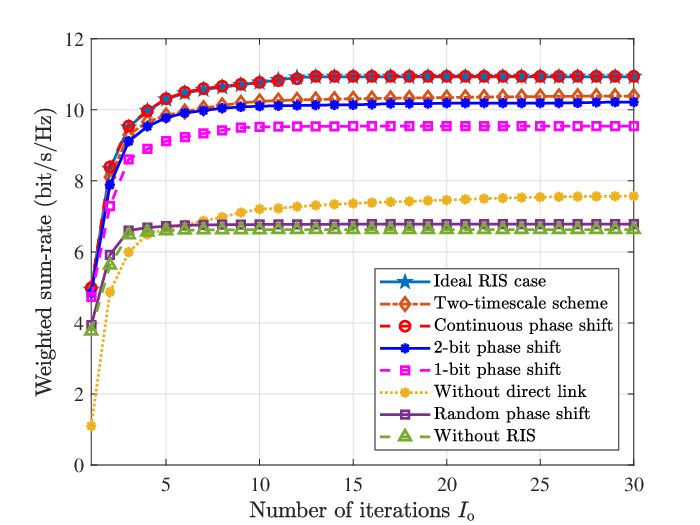
To show the convergency of the proposed algorithms, we plot the wsr against the number of iterations in Fig. 7 by running algorithms once with random initializations. The simulation setups are same as those used in Subsection VI-B, and we fix the distance as . To evaluate the convergency in non-ideal RIS phase shift cases, we add the curves “Continuous phase shift”, “1-bit phase shift”, and “2-bit phase shift” to denote the cases and . The results in Fig. 7 illustrate that, when the convergence error is no more than , the proposed joint precoding framework can converge within 15 iterations. To be more specific, the ideal ris case, two-timescale scheme, continuous phase shift case, and the case without direct links can converge within 15 iterations, while the discrete phase shift case can converge within 10 iterations. Since the conventional cell-free network without RIS and the scheme “Random phase shift” do not need to address the RIS precoding, the WSR in these cases can converge within 5 iterations. The results also indicate that, although the approximation operation in (52) causes the uncertainty of convergence, the proposed framework still enjoys a fast global convergence. More importantly, we find that the curves “Ideal RIS case” and “Continuous phase shift” are very close. The essential reason is that, for “Ideal RIS case”, actually most of the optimized RIS elements have an amplitude equal to 1. It indicates that, for the precoding design of the amplitude-uncontrollable RIS, we can simply relax its constant-modulus constraint and optimize its precoding as an ideal RIS. Then, we can directly project the optimized precoding matrix to the constant-modulus and obtain the final design. In this way, the optimization of RIS precoding becomes simple and low-complexity. Besides, it also implies that there is no need to design an amplitude-controllable ris for wireless communications.
VI-D Robustness of the joint precoding to CSI error
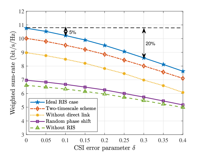
Generally, in the proposed RIS-aided cell-free system, the channel estimation is very challenging due to the high-dimensional channels. Here we analyze the robustness of the proposed joint precoding scheme to CSI error. To generate the imperfect channels, we model the practically estimated channel as [45]
| (55) |
where denotes the real channel and represents the estimation error with Gaussian distribution and zero mean, i.e. . We assume the variance , i.e. the error power, satisfies wherein denotes the ratio of the error power to the channel gain , which characterizes the level of CSI error. Then, using the same setups in Subsection VI-C, we plot the WSR against the CSI error parameter in Fig. 8. From this figure, we can observe that, the performance loss grows with the increasing of . Particularly, for the “Ideal RIS case”, compared with the perfect CSI without error (i.e. ), the system performance suffers a loss of when the error power is of the channel gain (i.e. ), and a loss of when . Thereby, the proposed joint precoding scheme shows strong robustness to CSI error.
VI-E The impact of key system parameters
To reveal more insights of the proposed RIS-aided cell-free network with different system parameters, we consider a new simulation scenario with more dispersed users and reset the locations of the four users in Fig. 5 as , , , and , respectively.
VI-E1 WSR against BS transmit power
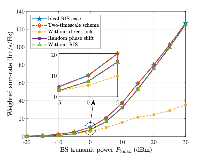
By fixing , we present the average weighted sum-rate against the bs transmit power in Fig. 9. From this figure we can observe that, with the increase of the bs transmit power, the weighted sum-rate rises rapidly in all cases. Particularly, “Two-timescale scheme” achieves very similar performance to “Ideal RIS case”. It indicates that, the RIS-aided channels of the unmatched user-RIS pairs indeed have negligible contribution to capacity improvement, which demonstrates the effectiveness of the proposed two-timescale joint precoding scheme. Besides, we have an important finding that, the performance gain brought by riss is significant only when the BS transmit power is moderate (e.g., form 0 dBm to 20 dBm), while the performance gain becomes negligible when the BS transmit power is too low (e.g. -20 dBm) or too high (e.g. 30 dBm). We explain this phenomenon in detail as follows.
Intuitively, when the BS transmit power is too low, the reflected signals by RIS are so weak that RISs have little contribution to performance improvement. While, when the BS transmit power is too high, the BSs prefer to allocate most of the power to the beams towards the BS-user links rather than the beams towards the BS-RIS-user links, which makes the role of riss less obvious. To be specific, as we can observe from Fig. 9, “Without direct link” can be roughly regarded as the scheme when the BSs allocate all power to the BS-RIS-user links, while “Without RIS” denotes the scheme when the BSs allocate all power to the BS-user links [32]. With the increasing of BS transmit power, the performance gap between these two schemes becomes larger and larger. It indicates that, compared with the first scheme (i.e. BSs allocate all power to the BS-user links), the benefit of applying the second scheme (i.e. BSs allocate all power to the BS-RIS-user links) is relatively lower and lower. When the BS transmit power is large enough, the performance can obtain much more gain from BS allocating power to BS-user link than to BS-RIS-user link, since the performance gap between them is too large. In this case, the BS will tend to allocate most of its power to the beam towards the BS-user link, which weakens the role of RIS.
VI-E2 WSR against number of RIS elements

Using the same setups as above, we present the average weighted sum-rate against the number of RIS elements in Fig. 10. We can observe that, the wsr of the proposed RIS-aided cell-free network increases as the number of ris elements rises. More importantly, we find that, with the increasing of ris elements, the approximation loss of the low-resolution phase shift becomes larger. For instance, when , the approximation loss in the case “1-bit phase shift” is about of the ideal case, and this loss grows to when . The observation implies that, when the number of ris is large, is is necessary to use more accurate phase shifts for passive precoding, so that the signals reflected from riss can reach the users more precisely. In addition, since the dimension of is , the complexity of solving (35) grows with the number of ris elements , and too more RIS elements will also make the channel estimations more challenging. Thus, it is essential to choose the ris element number reasonably.
VI-E3 WSR with different allowable matched user-RIS pairs
To evaluate the performance of the proposed two-timescale extension of the joint precoding scheme, in this part, we analyze the system WSR with different , which denotes the maximum number of RISs that each user can be matched with. To show more insights, in the same simulation scenario shown in Fig. 5, we reset the total number of RISs as and the RIS elements as . We further assume that the -th RIS is located at . Then, we plot the WSR against the distance with different in Fig. 11.
From this figure, we can observe that, the WSR increases as each user can be matched with more RISs. Compared with the ideal joint precoding design which acquires and utilizes all RIS-aided channels, the proposed two-timescale scheme suffers performance but consumes much less overhead for CSI acquisitions. For example, when , i.e. each user can be matched with at most 3 RISs, compared with the perfect joint precoding design to some extent, the proposed two-timescale scheme acquires and utilizes no more than RIS-aided channels for joint precoding design but only suffers an averaged capacity loss of about . Particularly, at the positions from to , the two-timescale scheme () can almost achieve the same performance as the ideal joint precoding design. In this way, the proposed two-timescale scheme consumes much less overhead for acquiring RIS-aided channels from the long-term perspective [22]. Thus, we can conclude that, the proposed two-timescale scheme can serve as a efficient scheme for balancing the performance and overhead for CSI acquisitions, which is especially suitable to employ in the cell-free networks with a large number of distributed RISs.

VI-F Trade-off between the number of BSs and RISs
Since deploying more RISs can improve the network capacity with low cost and power consumption, in this subsection we analyze the trade-off between the number of BSs and RISs.
To fairly evaluate the losses and gains, here we take the energy efficiency as the performance metric. According to the power consumption model developed in [15], the system energy efficiency is given by
| (56) |
where is the efficiency of the transmit power amplifier, while , , and denote the hardware power consumption at each BS, each user, and each RIS element, respectively.
For the simulation setups, we consider the same settings as those in [15], i.e. , dBW, dBm and dBm. To find more essential insights, we reset some parameters as and . We fix the distance-dependent effects by setting the related distances as m and m. By performing Algorithm 1 in ideal RIS case, we plot the energy efficiency against the number of BSs and that of RISs in Fig. 12. From this figure, we can observe that, given , the energy efficiency can be significantly improved by increasing the number of RISs . Particularly, when and , the maximal energy efficiency can be achieved, i.e. bit/s/Hz/W. However, when is too large, the energy efficiency will decline after deploying more RISs. For example, given , the system energy efficiency decreases to bit/s/Hz/W when , which is about a 34.8% loss. The reason is that, when the network capacity is large enough, the capacity improvement via deploying more RISs cannot make up for the extra power consumption. Therefore, carefully designing the trade-off between the number of BSs and RISs is the guarantee for balancing the capacity and power consumption in practical systems.

VII Conclusions and Future Works
In this paper, we first propose the concept of RIS-aided cell-free network, which aims to improve the network capacity with low cost and power consumption. Then, for the proposed RIS-aided cell-free network, in a typical wideband scenario, we formulate the joint precoding design problem to maximize the weighted sum-rate to optimize the network capacity, subject to the transmit power constraint of bs and the phase shift constraint of ris. Finally, we propose a joint precoding framework to solve this problem. Since most of the considered scenarios in existing works are special cases of the general scenario in this paper, the proposed joint precoding framework can also serve as a general solution to maximize the capacity in most of existing RIS-aided scenarios. Simulation results demonstrate that, with the assist of low-cost and energy-efficient riss, the proposed RIS-aided cell-free network can realize higher capacity than the conventional cell-free network.
Compared with the traditional cell-free network, the proposed RIS-aided cell-free network can achieve wider signal coverage [13], higher spectrum [32], and higher energy efficiency [15]. For future works, some open problems are still worth further investigations. For example, some other important performance metrics such as the energy efficiency [15], BS transmit power [17], and user fairness [23] are left for future works. Besides, some new hardware architecture such as active RIS [46] can be considered to further enhance the capacity. In some specific scenarios such as the internet of vehicles, how to select the replaced BSs and optimize the placements of RISs is also an interesting research direction.
Another promising technique benefiting from the advance of meta-materials is large intelligent surface (LIS) [47, 48, 49]. Different from the passive RIS, LIS is considered as a quasi-continuous surface [47] which can actively achieve surface beamforming [48]. Moreover, the signal model of LIS is in continuous-integral form [47, 48, 49]. The introduction of LIS into cell-free network will bring many open problems, such as how to bridge the gap between discrete model and continuous model, which are also left for future works.
Appendix A PDS-based method for solving subproblem (24)
We consider to solve (24) via the PDS method [37]. Firstly, by introducing Lagrange multipliers and , the Lagrangian for the augmented problem of (24) can be written as
| (57) |
where the function vector is defined by with being .
Next, we introduce a superscript to each variable as the iteration index, and we have the iterative formulas of and written as
| (58) |
where the step length is a sufficiently small positive value and the iteration directions and are given by
| (59a) | ||||
| (59b) | ||||
wherein the auxiliary function is denoted by
By simultaneously optimizing and via (58) until convergence, the optimal can be finally obtained without need of the inversion operation for the high-dimensional matrix .
Remark 1
We discuss the computational complexity of solving (24). Since is a fixed diagonal matrix with elements being 1, we can simply derive that the complexity of computing is . Then, we can further obtain that the computational complexity of updating and via (58) are and , respectively. Let denote the required iteration number for convergence. Then the overall complexity of the applied PDS-based method is about .
Appendix B PDS-based method for solving subproblem (35)
We consider to solve (35) via the PDS method [37]. Similar to Appendix A, by introducing Lagrange multipliers and , the Lagrangian for the augmented problem of (35) can be derived as
| (62) |
where the function vector is defined by with and . Then, we have the iterative formulas of and written as
| (63) |
wherein denotes the sufficiently small step length and the iteration directions and are obtained by
| (64a) | ||||
| (64b) | ||||
Note that, the auxiliary function is defined as
By simultaneously optimizing and via (63) until convergence, the optimal can be finally obtained without need of the inversion operation for the high-dimensional matrix .
References
- [1] Z. Zhang and L. Dai, “Capacity improvement in wideband reconfigurable intelligent surface-aided cell-free network,” in Proc. 2020 IEEE 21st Int. Workshop on Signal Process. Advances in Wireless Commun. (IEEE SPAWC’20), May 2020, pp. 1–5.
- [2] D. López-Pérez, M. Ding, H. Claussen, and A. H. Jafari, “Towards 1 Gbps/UE in cellular systems: Understanding ultra-dense small cell deployments,” IEEE Commun. Surveys Tuts., vol. 17, no. 4, pp. 2078–2101, Fourthquarter 2015.
- [3] F. E. Idachaba, “5G networks: Open network architecture and densification strategies for beyond 1000x network capacity increase,” in Proc. 2016 Future Technol. Conf. (FTC’16), Dec. 2016, pp. 1265–1269.
- [4] M. Kamel, W. Hamouda, and A. Youssef, “Ultra-dense networks: A survey,” IEEE Commun. Surveys Tuts., vol. 18, no. 4, pp. 2522–2545, Fourthquarter 2016.
- [5] J. G. Andrews, X. Zhang, G. D. Durgin, and A. K. Gupta, “Are we approaching the fundamental limits of wireless network densification?” IEEE Commun. Mag., vol. 54, no. 10, pp. 1558–1896, Oct. 2016.
- [6] A. Lozano, R. W. Heath, and J. G. Andrews, “Fundamental limits of cooperation,” IEEE Trans. Inf. Theory, vol. 59, no. 9, pp. 5213–5226, Sep. 2013.
- [7] E. Nayebi, A. Ashikhmin, T. L. Marzetta, and H. Yang, “Cell-free massive MIMO systems,” in Proc. 2015 49th Asilomar Conf. Signals Sys. Comput. (ACSSC’15), Nov. 2015, pp. 695–699.
- [8] G. Interdonato, E. Björnson, H. Q. Ngo, P. Frenger, and E. G. Larsson, “Ubiquitous cell-free massive MIMO communications,” EURASIP J. Wireless Commun. Netw., pp. 197–206, 2019.
- [9] H. Q. Ngo, A. Ashikhmin, H. Yang, E. G. Larsson, and T. L. Marzetta, “Cell-free massive MIMO versus small cells,” IEEE Trans. Wireless Commun., vol. 16, no. 3, pp. 1834–1850, Mar. 2017.
- [10] S. Mosleh, H. Almosa, E. Perrins, and L. Liu, “Downlink resource allocation in cell-free massive MIMO systems,” in Proc. 2019 Int. Conf. Comput. Netw. Commun. (ICNC’19), Feb. 2019, pp. 883–887.
- [11] M. Attarifar, A. Abbasfar, and A. Lozano, “Modified conjugate beamforming for cell-free massive MIMO,” IEEE Commun. Lett., vol. 8, no. 2, pp. 616–619, Apr. 2019.
- [12] Y. Jin, J. Zhang, S. Jin, and B. Ai, “Channel estimation for cell-free mmwave massive MIMO through deep learning,” IEEE Trans. Veh. Technol., vol. 68, no. 10, pp. 10 325–10 329, Oct. 2019.
- [13] Y. Liang, R. Long, Q. Zhang, J. Chen, H. V. Cheng, and H. Guo, “Large intelligent surface/antennas (LISA): Making reflective radios smart,” J. Commun. Inf. Networks, vol. 4, no. 2, pp. 40–50, Jun. 2019.
- [14] E. Basar, M. Di Renzo, J. De Rosny, M. Debbah, M. Alouini, and R. Zhang, “Wireless communications through reconfigurable intelligent surfaces,” IEEE Access, vol. 7, pp. 116 753–116 773, Aug. 2019.
- [15] C. Huang, A. Zappone, G. C. Alexandropoulos, M. Debbah, and C. Yuen, “Reconfigurable intelligent surfaces for energy efficiency in wireless communication,” IEEE Trans. Wireless Commun., vol. 18, no. 8, pp. 4157–4170, Aug. 2019.
- [16] M. Di Renzo, K. Ntontin, J. Song, F. H. Danufane, X. Qian, F. Lazarakis, J. De Rosny, D. Phan-Huy, O. Simeone, R. Zhang, M. Debbah, G. Lerosey, M. Fink, S. Tretyakov, and S. Shamai, “Reconfigurable intelligent surfaces vs. relaying: Differences, similarities, and performance comparison,” IEEE Open J. Commun. Soc., vol. 1, pp. 798–807, Jun. 2020.
- [17] Q. Wu and R. Zhang, “Beamforming optimization for wireless network aided by intelligent reflecting surface with discrete phase shifts,” IEEE Trans. Commun., vol. 68, no. 3, pp. 1838–1851, Mar. 2020.
- [18] P. Wang, J. Fang, X. Yuan, Z. Chen, and H. Li, “Intelligent reflecting surface-assisted millimeter wave communications: Joint active and passive precoding design,” IEEE Trans. Veh. Tech., vol. 69, no. 12, pp. 14 960–14 973, Dec. 2020.
- [19] C. Pan, H. Ren, K. Wang, W. Xu, M. Elkashlan, A. Nallanathan, and L. Hanzo, “Multicell MIMO communications relying on intelligent reflecting surfaces,” IEEE Trans. Wireless Commun., vol. 19, no. 8, pp. 5218–5233, Aug. 2020.
- [20] C. Huang, C. Zhang, J. Yang, B. Sun, B. Zhao, and X. Luo, “Reconfigurable metasurface for multifunctional control of electromagnetic waves,” Adv. Opt. Mater., vol. 5, no. 22, p. 1700485, Sep. 2017.
- [21] Ö. Özdogan, E. Björnson, and E. G. Larsson, “Intelligent reflecting surfaces: Physics, propagation, and pathloss modeling,” IEEE Wireless Commun. Lett., vol. 9, no. 5, pp. 581–585, May 2020.
- [22] C. Hu, L. Dai, S. Han, and X. Wang, “Two-timescale channel estimation for reconfigurable intelligent surface aided wireless communications,” IEEE Trans. Commun. (early access), Apr. 2021.
- [23] Q.-U.-A. Nadeem, A. Kammoun, A. Chaaban, M. Debbah, and M.-S. Alouini, “Asymptotic max-min SINR analysis of reconfigurable intelligent surface assisted MISO systems,” IEEE Trans. Commun., vol. 19, no. 12, pp. 7748–7764, Dec. 2020.
- [24] L. Dai, B. Wang, M. Wang, X. Yang, J. Tan, S. Bi, S. Xu, F. Yang, Z. Chen, M. D. Renzo, C. B. Chae, and L. Hanzo, “Reconfigurable intelligent surface-based wireless communications: Antenna design, prototyping, and experimental results,” IEEE Access, vol. 8, pp. 45 913–45 923, Mar. 2020.
- [25] Q. Wu and R. Zhang, “Intelligent reflecting surface enhanced wireless network: Joint active and passive beamforming design,” in Proc. 2018 IEEE Global Commun. Conf. (IEEE GLOBECOM’18), Dec. 2018, pp. 1–6.
- [26] C. Huang, A. Zappone, M. Debbah, and C. Yuen, “Achievable rate maximization by passive intelligent mirrors,” in Proc. 2018 IEEE Int. Conf. on Acoustics, Speech and Signal Process. (IEEE ICASSP’18), Apr. 2018, pp. 3714–3718.
- [27] B. Di, H. Zhang, L. Song, Y. Li, Z. Han, and H. V. Poor, “Hybrid beamforming for reconfigurable intelligent surface based multi-user communications: Achievable rates with limited discrete phase shifts,” IEEE J. Sel. Areas Commun., vol. 38, no. 8, pp. 1809–1822, Aug. 2020.
- [28] H. Li, R. Liu, M. Liy, Q. Liu, and X. Li, “IRS-enhanced wideband MU-MISO-OFDM communication systems,” in Proc. 2020 IEEE Wireless Commun. and Networking Conf. (WCNC’20), May 2020, pp. 1–6.
- [29] Y. Yang, S. Zhang, and R. Zhang, “IRS-enhanced ofdm: Power allocation and passive array optimization,” in Proc. 2019 IEEE Global Commun. Conf. (IEEE GLOBECOM’19), Dec. 2019, pp. 1–6.
- [30] U. Siddique, H. Tabassum, and E. Hossain, “Downlink spectrum allocation for in-band and out-band wireless backhauling of full-duplex small cells,” IEEE Trans. Commun., vol. 65, no. 8, pp. 3538–3554, Aug. 2017.
- [31] Y. Han, S. Zhang, L. Duan, and R. Zhang, “Cooperative double-IRS aided communication: Beamforming design and power scaling,” IEEE Wireless Commun. Lett., vol. 9, no. 8, pp. 1206–1210, Aug. 2020.
- [32] Q. Wu and R. Zhang, “Intelligent reflecting surface enhanced wireless network via joint active and passive beamforming,” IEEE Trans. Wireless Commun., vol. 18, no. 11, pp. 5394–5409, Nov. 2019.
- [33] Q. Zheng, Y. Li, Y. Han, Y. Jing, M. Feng, Y. Pang, J. Wang, H. Ma, S. Qu, and J. Zhang, “Ultra-wideband side-lobe level suppression using amplitude-adjustable metasurfaces,” J. Physics D: Applied Physics, vol. 52, no. 6, p. 065102, Dec. 2018.
- [34] K. Shen and W. Yu, “Fractional programming for communication systems—part I: Power control and beamforming,” IEEE Trans. Signal Process., vol. 66, no. 10, pp. 2616–2630, May 2018.
- [35] W. Dinklebach, “On nonlinear fractional programming,” Manag. Science, vol. 13, no. 7, pp. 492–498, Oct. 2014.
- [36] S. Boyd, N. Parikh, E. Chu, B. Peleato, and J. Eckstein, “Distributed optimization and statistical learning via the alternating direction method of multipliers,” Nov. 2014, [Online] Available: https://stanford.edu/~boyd/papers/pdf/admm_distr_stats.pdf.
- [37] S. Boyd, “Subgradient methods,” May 2014, [Online] Available: https://web.stanford.edu/class/ee364b/lectures/subgrad_method_notes.pdf.
- [38] H. Guo, Y. Liang, J. Chen, and E. G. Larsson, “Weighted sum-rate maximization for reconfigurable intelligent surface aided wireless networks,” IEEE Trans. Wireless Commun., vol. 19, no. 5, pp. 3064–3076, May 2020.
- [39] K. G. Murty and S. N. Kabadi, “Some NP-complete problems in quadratic and nonlinear programming,” Math. Program., vol. 39, pp. 117–129, Jun. 1987.
- [40] T. Nie, S.-C. Fang, Z. Deng, and J. E. Lavery, “On linear conic relaxation of discrete quadratic programs,” Optimization Methods and Software, vol. 31, pp. 737–754, Jan. 2016.
- [41] K. C. Toh, M. J. Todd, and R. H. Tütüncü, “SDPT3 — a Matlab software package for semidefinite programming, version 1.3,” Optimiz. Methods Softw., vol. 11, no. 1-4, pp. 545–581, Jan. 2008.
- [42] Z. Yang, L. Xie, and C. Zhang, “A discretization-free sparse and parametric approach for linear array signal processing,” IEEE Trans. Signal Process., vol. 62, no. 19, pp. 4959–4973, Oct. 2014.
- [43] Y. Sun, P. Babu, and D. P. Palomar, “Majorization-minimization algorithms in signal processing, communications, and machine learning,” IEEE Trans. Signal Process., vol. 65, no. 3, pp. 794–816, Aug. 2017.
- [44] K. Alhujaili, V. Monga, and M. Rangaswamy, “Transmit MIMO radar beampattern design via optimization on the complex circle manifold,” IEEE Trans. Signal Process., vol. 67, no. 13, pp. 3561–3575, May 2019.
- [45] P. Ubaidulla and A. Chockalingam, “Relay precoder optimization in MIMO-relay networks with imperfect CSI,” IEEE Trans. Signal Process., vol. 59, no. 11, pp. 5473–5484, Aug. 2011.
- [46] Z. Zhang, L. Dai, X. Chen, C. Liu, F. Yang, R. Schober, and H. V. Poor, “Active RIS v.s. passive RIS: Which will prevail in 6G?” arXiv preprint arXiv:2103.15154, Mar. 2021.
- [47] C. Huang, S. Hu, G. C. Alexandropoulos, A. Zappone, C. Yuen, R. Zhang, M. D. Renzo, and M. Debbah, “Holographic MIMO surfaces for 6G wireless networks: Opportunities, challenges, and trends,” IEEE Trans. Wireless Commun., vol. 27, no. 5, pp. 118–125, Oct. 2020.
- [48] D. Dardari, “Communicating with large intelligent surfaces: Fundamental limits and models,” IEEE J. Sel. Areas Commun., vol. 38, no. 11, pp. 2526–2537, Nov. 2020.
- [49] J. Yuan, H. Q. Ngo, and M. Matthaiou, “Towards large intelligent surface (LIS)-based communications,” IEEE Trans. Commun., vol. 68, no. 10, pp. 6568–6582, Oct. 2020.
![[Uncaptioned image]](2002.03744v3/Zijian_Zhang.png) |
Zijian Zhang (S’20) received the B.E. degree in electronic engineering from Tsinghua University, Beijing, China, in 2020. He is currently working toward the Ph.D. degree in electronic engineering from Tsinghua University, Beijing, China. His research interests include physical-layer algorithms for massive MIMO and reconfigurable intelligent surfaces (RIS). He has received the National Scholarship in 2019 and the Excellent Thesis Award of Tsinghua University in 2020. |
![[Uncaptioned image]](2002.03744v3/LinglongDai_Photo.png) |
Linglong Dai (M’11-SM’14) received the B.S. degree from Zhejiang University, Hangzhou, China, in 2003, the M.S. degree (with the highest honor) from the China Academy of Telecommunications Technology, Beijing, China, in 2006, and the Ph.D. degree (with the highest honor) from Tsinghua University, Beijing, China, in 2011. From 2011 to 2013, he was a Postdoctoral Research Fellow with the Department of Electronic Engineering, Tsinghua University, where he was an Assistant Professor from 2013 to 2016 and has been an Associate Professor since 2016. His current research interests include reconfigurable intelligent surface (RIS), massive MIMO, millimeter-wave/ Terahertz communications, and machine learning for wireless communications. He has coauthored the book “MmWave Massive MIMO: A Paradigm for 5G” (Academic Press, 2016). He has authored or coauthored over 60 IEEE journal papers and over 40 IEEE conference papers. He also holds 19 granted patents. He has received five IEEE Best Paper Awards at the IEEE ICC 2013, the IEEE ICC 2014, the IEEE ICC 2017, the IEEE VTC 2017-Fall, and the IEEE ICC 2018. He has also received the Tsinghua University Outstanding Ph.D. Graduate Award in 2011, the Beijing Excellent Doctoral Dissertation Award in 2012, the China National Excellent Doctoral Dissertation Nomination Award in 2013, the URSI Young Scientist Award in 2014, the IEEE Transactions on Broadcasting Best Paper Award in 2015, the Electronics Letters Best Paper Award in 2016, the National Natural Science Foundation of China for Outstanding Young Scholars in 2017, the IEEE ComSoc Asia-Pacific Outstanding Young Researcher Award in 2017, the IEEE ComSoc Asia-Pacific Outstanding Paper Award in 2018, the China Communications Best Paper Award in 2019, the IEEE Access Best Multimedia Award in 2020, and the IEEE Communications Society Leonard G. Abraham Prize in 2020. He was listed as a Highly Cited Researcher by Clarivate Analytics in 2020. He is an Area Editor of IEEE Communications Letters, and an Editor of IEEE Transactions on Communications and IEEE Transactions on Vehicular Technology. Particularly, he is dedicated to reproducible research and has made a large amount of simulation codes publicly available. |